Sparse Generalized Yule–Walker Estimation for Large Spatio-temporal Autoregressions with an Application to NO2 Satellite Data
Abstract
We consider a high-dimensional model in which variables are observed over time and space. The model consists of a spatio-temporal regression containing a time lag and a spatial lag of the dependent variable. Unlike classical spatial autoregressive models, we do not rely on a predetermined spatial interaction matrix, but infer all spatial interactions from the data. Assuming sparsity, we estimate the spatial and temporal dependence fully data-driven by penalizing a set of Yule-Walker equations. This regularization can be left unstructured, but we also propose customized shrinkage procedures when observations originate from spatial grids (e.g. satellite images). Finite sample error bounds are derived and estimation consistency is established in an asymptotic framework wherein the sample size and the number of spatial units diverge jointly. Exogenous variables can be included as well. A simulation exercise shows strong finite sample performance compared to competing procedures. As an empirical application, we model satellite measured concentrations in London. Our approach delivers forecast improvements over a competitive benchmark and we discover evidence for strong spatial interactions.
Keywords: Spatio-Temporal Models, SPLASH, Satellite Data, Yule-Walker, High-Dimensional
JEL-Codes: C33, C53, C55
1 Introduction
Spatio-temporal models are powerful tools to explain and exploit dependencies between variables that are observed over both time and space, but they come with a number of challenges. In particular, endogeneity issues arise because the contemporaneous observations occur on both sides of the model equation. Furthermore, the inclusion of both spatial and temporal lags quickly results in heavily parameterized models. To circumvent these issues, a large part of the literature incorporates predetermined spatial weight matrices that govern the contemporaneous interactions between spatial units. Examples of this modelling strategies are: the spatial autoregressive model with a Gaussian quasi-maximum likelihood estimator (QMLE) by Lee, 2004; the QMLE estimation of stationary spatial panels with fixed effects detailed in Yu et al., 2008; the extension of these spatial panels to include spatially autoregressive disturbances as in Lee and Yu, 2010; a further extension to a non-stationary setting in which units can be spatially cointegrated in Yu et al., 2012; and the computationally beneficial generalized method of moments (GMM) estimator by Lee and Yu, 2014. While the choice of the spatial weight matrix is a key element of the model specification, its selection process can feel somewhat arbitrary and/or tedious. The arbitrariness might prevail when practical considerations fail to suggest a particular mechanism for the spatial interactions. Accordingly, more recent literature focuses on either incorporating multiple weight matrices (Debarsy and LeSage, 2018; Zhang and Yu, 2018, e.g.) or, at the expense of estimating many parameters, directly inferring all spatial interactions from the data (Lam and Souza, 2019; Gao et al., 2019; Ma et al., 2021, e.g.). We contribute to the latter strand of literature with the development of a new estimator that provides several unique benefits.
In this paper, we propose the SPatial LAsso-type SHrinkage (SPLASH) estimator as a fully data-driven estimator of spatio-temporal interactions. Apart from a generous bandwidth upper bound, this SPLASH estimator leaves the spatial weight matrix and autoregressive matrix unspecified while employing a lasso approach to recover sparse solutions. Building upon previous works by Dou et al., 2016 and Gao et al., 2019, we resolve the endogeneity problem in our spatio-temporal regressions by estimating the generalized Yule-Walker equations. Our contributions are five-fold. First, assuming sparsity in the coefficient matrices and general mixing conditions on the innovations, we derive finite-sample performance bounds for the estimation and prediction error of our estimator. We subsequently utilize these bounds to derive asymptotic consistency in a variety of settings. For example, in the special case of a finitely bounded bandwidth and unstructured sparsity, it follows that the number of spatial units may grow at any polynomial rate of the number of temporal observations . Second, we adopt a banded estimation procedure for the autocovariance matrices that underlie the generalized Yule-Walker equations. The faster convergence rates of these banded autocovariance matrix estimators are shown to translate into better convergence rates of our SPLASH estimator. Third, we show that dependence between neighbouring units that are ordered on a spatial grid translates to diagonally structured forms of sparsity in the spatial weight matrix. A tailored regularization procedure reminiscent of the sparse group lasso is proposed. Fourth, we generalize the model to include exogenous variable and demonstrate that an extended system of Yule-Walker equations continues to provide consistent estimators. Our simulation study confirms these points. Fifth and final, we employ SPLASH to predict concentrations in London from satellite data.
Elaborating on the empirical application, we collect daily column densities from August 2018 to October 2020, recorded by the TROPOspheric Monitoring Instrument (TROPOMI) on board of the Corpernicus Sentinel-5 Precursor satellite. Each spatial unit is an aggregation of a small number of pixels on the satellite image. We find that SPLASH constructs more accurate one-step ahead predictions for all spatial units compared to the procedure in Gao et al., 2019, while outperforming a competitive penalized VAR benchmark for the majority of spatial units. In addition, we find evidence for spatial interactions between first-order neighbours and second-order neighbours (i.e. neighbours of neighbours).
There are two strands of literature that are closely linked to this work: the literature on the estimation of (nonparametric) spatial weight matrices and the literature on spatio-temporal vector autoregressions. Some similarities and differences are as follows. Lam and Souza, 2014 consider a model specification where the spatial units depend linearly on a spatial lag and exogenous regressors. The adaptive lasso is proven to select the correct sparsity pattern. To solve the endogeneity issue, they require the error variance to decay to zero as the time dimension grows large. Ahrens and Bhattacharjee, 2015 solve the endogeneity problem using external instruments. Their two-step lasso estimation procedure selects the relevant instruments in the first step and the relevant spatial interactions in the second step. The theoretical properties of this estimator are derived using moderate deviation theory as in Jing et al., 2003. This approach requires the instruments and the idiosyncratic component to be serially independent. Clearly, a serial independence assumption is unrealistic for the spatio-temporal models we consider here. Finally, Lam and Souza, 2019 augment a spatial lag model with a set of potentially endogenous variables (the augmenting set). They decompose the spatial weight matrix into a pre-determined component based on expert knowledge and a sparse adjustment matrix that represents specification errors. The adjustment matrix is sparsely estimated based on a penalized version of instrumental variables (IV) regression. If these instrumental variables are selected as temporal lags of the dependence variable, then their IV regressions are similar to generalized Yule-Walker estimation. In contrast to our approach, Lam and Souza, 2019 do not regularize the interactions between the dependent variables and the variables in the augmenting set, and they assume the number of such interactions to be fixed. A fixed number of interactions is inappropriate in high-dimensional settings in which the number of spatial units is allowed to diverge.
Closest related to the our work are Gao et al., 2019, and Ma et al., 2021. Both papers consider the same model and an estimation procedure that relies on generalized Yule-Walker equations. The key difference with our paper lies in the method by which the model complexity is controlled during estimation. Gao et al., 2019 assume the coefficient matrices to be banded with a bandwidth that is small compared to the number of spatial units. The bandwidth is determined from the data and all parameters within the selected bandwidth are left unregularized. Our SPLASH estimator, however, has the ability to exploit (structured) sparsity within the bandwidth and thereby improve estimation and forecasting performance. In addition, apart from a generous upper bound on the bandwidth to ensure identification, SPLASH does not require an a priori choice regarding the bandwidth. The recently developed bagging approach in Ma et al., 2021 does allow for sparsity within the bands, yet it also requires the calculation of so-called solution paths. That is, a forward addition and backward deletion stage are needed to determine the variables that enter the final model specification. In contrast, the SPLASH estimator provides this solution at once. Furthermore, their approach is not designed to detect diagonally structured forms of sparsity, while the ability to do so results in clear performance improvements of SPLASH in both the simulations and the empirical application considered below.
This paper is organized as follows. Section 2 introduces the spatio-temporal vector autoregression and the banded autocovariance estimator that underlies the generalized Yule-Walker estimation approach. The SPLASH estimator and its theoretical properties are discussed in Section 3. The simulation results in Section 4 and the empirical application in Section 5 demonstrate the benefits of the SPLASH estimator. Section 6 concludes.
Notation
The indicator function equals 1 if is true and zero otherwise. For a vector , the -norm of is denoted , with as an important special case. The total number elements in is denoted by and the number of non-zero elements in is denoted by . The Orlicz norm is defined as for any being a convex, increasing function with and as . In addition, we rely on several matrix norms. For a matrix , the matrix norms induced by the vector -norms are given by . Noteworthy examples are: , the spectral norm where stands for the maximum eigenvalue, and . The Frobenius norm of is . Finally, we define and . Let denote an index set with cardinality . Then, denotes the -dimensional vector with the elements of indexed by , whereas denotes the -dimensional matrix containing the columns of indexed by . In addition, we define as the collections of elements lying on (pairs of) the diagonals in the matrix . Finally, is a generic constant that can change value from line-to-line.
2 The Spatio-temporal Vector Autoregression
As in the recent paper by Gao et al., 2019, we consider the spatio-temporal vector autoregression
| (1) |
where stacks the observations at time over a collection of spatial units. The contemporaneous spatial dependence between these spatial units is governed by the matrix with for . The matrix incorporates dependence on past realizations. Finally, we have the innovation vector . We impose the following assumptions on the DGP in (1).
Assumption 1 (Stability).
- (a)
.
- (b)
and .
Remark 1.
Assumption 1 is defined in terms of . Since for any matrix , the norm is convenient when bounding products of matrices containing transposes.
Assumption 2 (Innovations).
- (a)
The sequence is a covariance stationary, martingale difference process with respect to the filtration , and geometrically strong mixing (-mixing). That is, the mixing coefficients satisfy for all and some constants . The largest and smallest eigenvalues of are bounded away from and .
- (b)
Either one of the following assumptions holds:
- (b1)
For , we require for .
- (b2)
For , we have .
- (b1)
Assumption 1 ensures that has a stable reduced form VAR(1) specification. This follows from the following two observations. First, Assumption 2(a) bounds the maximum row and column sums of and thereby constraints the contemporaneous dependence between the time series. This assumption reminds of the spatial econometrics literature in which the spatial parameter is bounded from above and the prespecified spatial weight matrix is standardized (see, e.g. Lee, 2004 and Lee and Yu, 2010). Typically, the product – the natural counterpart of the matrix – is required to fulfil conditions similar to .11 1 For instance, it is not uncommon to row-normalize (each absolute row sum equal to 1) and restrict , see pages 1903-1904 of Lee, 2004. If is symmetric, then also . Invertibility of is guaranteed because and we have the reduced-form representation with and . From , we infer that the absolute row and column sum of are bounded. The latter is the logical counterpart of assumption B2 in Dou et al., 2016. Second, Assumption 2(b) controls serial dependence. Indeed, we conclude from that both unit root and explosive behaviour of the reduced form specification are ruled out. The resulting stable VAR(1) representation is convenient to study the theoretical properties of our penalized estimator.
The assumptions on the innovation process , Assumption 2, are closely related to those in Masini et al., 2019. Assumption 2(a) places restrictions on the time series properties of the error term through martingale difference (m.d.) and mixing assumptions. The m.d. assumption implies that while the mixing assumption controls the serial correlation in the data. Polynomial or exponential tail decay of the distribution of the innovations is imposed through either Assumption 2(b1) or Assumption 2(b2), respectively. The type of tail decay will directly influence the growth rates we can allow for and . The discussions in Masini et al., 2019 demonstrate that Assumption 2 allows for a wide range of innovation models.
Any further structure being absent, there are unknown parameters in and to estimate. Three complications are encountered when estimating these parameters. First, if , then occurs on both sides of the equation, and we face an endogeneity problem which renders OLS estimation inconsistent. Second, the number of unknown parameters grows quadratically in the cross-sectional dimension . The model thus quickly becomes too large to estimate accurately without regularization. Finally, the multitude of parameters raises concerns about identifiability. These three complications are addressed by: (1) imposing structure on the matrices and , and (2) estimating the unknown coefficients using the Yule-Walker equations (e.g. Brockwell and Davis, 1991, p. 420).
There are several possibilities to introduce structure into and . Early spatial econometrics models, e.g. the spatial autoregressive (SAR) model or spatial Durbin model (SDM), incorporate spatial effects through the product (with pre-specified). The specification imposes substantial structure on and leaves only the single parameter to estimate. Dou et al., 2016 consider a more general setting in which each row of receives its own spatial autoregressive parameter. Specifically, they set and , and estimate the coefficients in . Gao et al., 2019 require and to be banded matrices.22 2 The matrix has bandwidth if the total number of nonzero entries in any row or column is at most . We employ a similar assumption.
Assumption 3 (Banded matrices).
Recall , , and . We have: (a) for all with , and (b) for all .
Assumption 3 serves two purposes. First, for each spatial unit , the matrices and are banded to have no more than unknown parameters per equation. With moment conditions for each , Assumption 3(a) is key in identifying the parameters. Our discussions in Section 3 illustrate that this assumption is realistic when the data is observed on a regular grid. The combination of Assumptions 3(a)–(b) is exploited in the Yule-Walker estimation approach. This approach requires estimation of the autocovariance matrices . Especially in our large settings, it is crucial to rely on covariance matrix estimators that converge at a fast rate. If , , and are banded, then the following result applies.
Theorem 1 (Convergence rates for banded sample autocovariance matrices).
For any matrix , its -banded counterpart is defined as . Define the matrix with and , and choose
| (2) | ||||
then with a probability of at least
- (a)
- (b)
where
for some , and
All constants (, , , etc.) are positive and independent of and . The proof (see the Appendix) shows how these constants are related to quantities in Assumptions 1–3.
Theorem 1 shows that banded estimators for and provide an accurate approximation to . Each of these banded matrices has at most nonzero elements in their columns/rows. In other words, given , and , Assumptions 1–3 guarantee that and can be well-approximated by matrices with bandwidths smaller than . This improves the convergence rate of our estimator.
3 Sparse Estimation
3.1 The SPLASH(,) Estimator
Even under Assumption 3, the number of unknown parameters in and continues to grow quadratically in . For large , the accurate estimation of all these parameters becomes infeasible rather quickly. To alleviate this curse of dimensionality, we rely on sparsity. Sparsity naturally occurs when two spatial units do not interact with each other. We demonstrate, however, that a special, and exploitable, sparsity pattern arises whenever the spatial units are ordered in a structured way.


As an illustrative example, let us consider repeated measurements on the spatial grids shown in the left column of Figure 1. The spatial units are labelled up to and enumerated row-wise. This ordering of the spatial entities creates an implicit notion of proximity and we intuitively expect economic/physical interactions to be most pronounced at short length scales. In Figure 1(a) we start from the situation in which the spatial units are restricted to communicate horizontally. Blue arrows indicate explicitly that interacts with , and interacts with both and . Such interactions occur among all elements in the grid. More importantly, if only these horizontal interaction exist, then the matrices and feature a sparsity pattern as shown in Figure 1(b). The blue elements are potentially nonzero whereas uncolored elements are zero. The nonzero elements in and are seen to cluster in specific, dense diagonals with the occasional zero when horizontal neighbours are absent (at the boundary of the grid). This diagonal sparsity pattern is not an artifact of allowing horizontal interactions only. Figures 1(c) adds the vertical interactions and the accompanying sparsity pattern again manifests itself along diagonals (Figure 1(d)). Finally, with diagonal nearest neighbours being horizontal neighbors of vertical elements, we observe a “thickening” of the diagonals in Figure 1(f). Guided by these considerations we combine generalized Yule-Walker estimation with a sparse group penalty (Simon et al., 2013, e.g.). The Yule-Walker estimator will control for endogeneity, while the sparse group penalty will shrink towards diagonal structures by including/omitting complete diagonals and thus selecting the required interactions. Compared to Gao et al., 2019, we hereby gain the ability to exploit sparsity within banded matrices.
A formal definition of our estimator requires further notation. Part of this notation comes naturally if we briefly review the generalized Yule-Walker estimator. After post-multiplying by and taking expectations, we find or, equivalently,
| (3) |
The th column of contains all coefficients that belong to the th equation in (1). Assumption 3 requires several of these coefficients to be zero so we exclude these from the outset. We collect all remaining (possibly) nonzero coefficients in the th equation in the vector , and define as the matrix containing the corresponding columns from . In the population, we have for . Sample counterparts of and are readily available from the sample autocovariance matrices. More explicitly, Gao et al., 2019 set and construct from the appropriate columns of . Motivated by , they define their estimator as the following minimizer:
| (4) |
We will adjust this objective function in three ways. First, we define our estimator in terms of banded estimated covariance matrices, which allows us to exploit the results in Theorem 1. Second, our group penalty penalizes parameters across equations so we can no longer estimate the parameters equation-by-equations. We therefore define and , with being constructed similarly to (see Figure 2 for an illustration).33 3 In general, all quantities derived from autocovariance matrices come in three versions: (1) the population quantity, (2) the estimated counterpart without banding denoted with an additional “hat”, and (3) the estimated counterpart with banding featuring both a “hat” and the subscript . In this notation, the expression defines the joint objective function that sums the individual contributions in (4) over all equations. Finally, we construct the penalty function. We define an index set that partitions the vector into sub-vectors, denoted , that contain the non-zero diagonals of and that are admissible under Assumption 3 as
| (5) |
respectively, and let . Based on this notation, we define our objective function as
| (6) |
The spatial lasso-type shrinkage estimator, abbreviated SPLASH(,) or SPLASH in short, is defined as the minimizer of (6), i.e. . The importance of the penalty function is governed by the penalty parameter and the second hyperparameter balances group-structured sparsity versus individual sparsity. At the extremities of we find the group lasso () and the lasso (). Intermediate values of will shrink both groups of diagonal coefficients in and and individual parameters. The SPLASH solution promotes completely sparse diagonals and sparse elements within nonzero diagonals, and thus shrinks towards sparsity patterns of the type displayed in Figure 1(b). As the structure of our estimator is similar to that of the Sparse Group Lasso (SGL), efficient algorithms are available to compute its solution (Simon et al., 2013, see, e.g.). An R/C++ implementation of the SPLASH estimator based on this algorithm is available on one of the author’s website.44 4 https://sites.google.com/view/etiennewijler/code.
3.2 Theoretical Properties of the SPLASH(,) Estimator
In this section we derive the theoretical properties of the SPLASH estimator. First, however, we require an additional assumption on the DGP in order to ensure that and in (1) are uniquely identified. To this end, we leverage the bandedness assumption in Assumption 3, which enables unique identification of and via a straightforward full-rank condition on sub-matrices of the autocovariance matrices that appear in the generalized Yule-Walker equations.
Assumption 4 (Restricted minimum eigenvalue).
Assume that
Assumption 4 states that every sub-matrix containing columns from has full column-rank and a minimum singular value bounded away from zero. Related assumptions appear in Bickel et al., 2009, who refer to as a restricted eigenvalue and use this quantity to construct sufficient conditions for their restricted eigenvalue assumptions. Assumption 4 fits our framework particularly well, as the assumed maximum bandwidth of the matrices and in Assumption 3 imply that the diagonal blocks of the matrix never contain more than unique columns of . Using this property, we show in Lemma 1 of Appendix A that a Sparse Group Lasso compatibility condition is implied by Assumption 4.
Equipped with Assumption 4, we find the following finite-sample performance bounds on the prediction and estimation error of SPLASH.
Theorem 2.
Theorem 2 contains a finite-sample performance bound on the prediction and estimation error for the SPLASH(,) estimator. It offers some interesting insights. First, we focus on the probability with which inequality (7) holds. For VAR estimation with a penalized least-squares objective function, such probabilities are governed by tail probabilities of the process (see, e.g. lemma 4 in Kock and Callot, 2015, or lemmas 5–6 in Medeiros and Mendes, 2016). Because Yule-Walker estimation relies primarily on autocovariance matrix estimation, our probability depends on the tail decay of the distribution of . Overall, the probability of (7) improves through faster tail decay of the innovation distribution (compare cases (a) and (b)) and banded autocovariance matrix estimation (Theorem 1). Second, we look closer at the performance upper bound itself. The right-hand side of (7) demonstrates that the upper bound of the prediction and estimation error is increasing in , which in turn is increasing in the bandwidths and , increasing in the group sizes (), and increasing in the number of relevant interactions (). Furthermore, the prediction and estimation error increases in the degree of penalization. Whereas this seemingly suggests to minimize as to improve performance bounds, we emphasize that the effect of regularization in Theorem 2 is two-fold: increasing regularization deteriorates the performance bound, but increases the probability of the set on which the performance bound holds. Intuitively, shrinkage induces finite-sample bias which worsens accuracy, but simultaneously reduces sensitivity to noise, thereby enabling performance guarantees at higher degrees of certainty.
The aforementioned effects can also be demonstrated by means of an asymptotic analysis. Based on Theorem 2, we derive the conditions for convergence of the prediction and estimation errors in the following corollary. The exact convergence rates are also provided.
Corollary 1.
Corollary 1 provides insights into the determinants of the convergence rate. In particular, the result confirms that the convergence rate decreases in the bandwidths and , the number of spatial units , the number of interactions and the degree of penalization .55 5 Recall that , such that a higher implies a faster decay of the penalty term. To ensure that the set on which the performance bound in Theorem 2 holds occurs with probability converging to one, conditions (i) and (ii) impose that the degree of penalization does not decay too fast. The optimal convergence rate is obtained by choosing as large as possible without violating these conditions. Some concrete examples are provided in Remark 2.
Remark 2.
Insightful special cases can be examined based on Corollary 1. For the sake of brevity, we consider two cases while focusing on the estimation error and assuming errors with at least finite moments (Assumption 2(b1)). In the absence of within-group shrinkage (), Corollary 1 demonstrates that , with by choosing arbitrarily close to 1. The estimator now converges almost at rate . For fixed and large , this is close to the common -rate of fixed-dimensional settings without regularization. If shrinkage is imposed at the individual interaction level only (, then and the estimation error converges almost at the rate . Noting that , we see that SPLASH(,) attains a convergence rate at least as fast SPLASH(,), and possibly faster when the sparsity is unstructured or the diagonals are highly sparse.
3.3 Exogenous variables
We generalize model specification (1) by accommodating exogenous variables, i.e.
| (8) |
Each vector augments the spatio-temporal vector autoregression with an extra regressor. This regressor may vary over time and it is exogenous, i.e. we have for . For notational brevity, we consider the situation in which the exogenous regressors can only directly influence spatial unit . This explains the diagonal structure in . In Remark 4 we argue that this simplification does not greatly hinder generality. In contrast to Ma et al., 2021, we allow to vary with location. We keep fixed.
To account for the exogenous variables, we modify the generalized Yule-Walker estimator of Section 3.1. We recall , and define the matrices and . Two sets of Yule-Walker equations, namely
| (9a) | |||
| and | |||
| (9b) | |||
are derived by post-multiplying the model by respectively and , and taking expectations. Compared to (3), the Yule-Walker equations in (9a) contain the additional term to provide information on . However, if (e.g. when and are independent and ), then (9a) alone will not identify . We therefore add the additional Yule-Walker equations in (9b). To develop the estimator, we combine (9a) and (9b) into
| (10) |
From this point onward, the development of the SPLASHX(,) estimator mimics the reasoning of page 4 closely. First, we focus on the th spatial unit and collect all the nonzero coefficients of and (as stipulated by Assumption 3) in . Letting denote the columns in related to and defining both and , result (10) implies
Second, we define (a) the sample counterparts of , and as respectively , and , and (b) define the quantities , and based on their underlying sample covariance matrix estimators. Finally, set , , and . The SPLASHX(,) objective function is
| (11) | ||||
This objective function allows for the estimation of , sparse coefficients, completely sparse vectors , and completely sparse diagonals in the coefficient matrices and . There is a clear mathematical resemblance between the SPLASH and SPLASHX estimators. Accordingly, under appropriate modifications to Assumptions 1–4, a finding similar to Theorem is attainable. We provide this result as Theorem 3 and refer the reader to Supplement for detailed assumptions and proofs.
Theorem 3.
Remark 3.
The inclusion of exogenous variables affects the autocovariance structure of the data. For example, if , then and
Clearly, now also depends on the various second moments of the exogenous covariates. We do not make any a priori assumptions on and thus define the SPLASHX(,) in terms of the unbanded autocovariance matrix estimators.
Remark 4.
Defining the coefficient matrix in front of as diagonal is not restrictive. That is, by letting be a reordered version of , the former’s addition to the model can accommodate for the situation in which the dependent variable is influenced by the exogenous variable from multiple locations.
4 Simulations
4.1 Simulation setting
In this section, we explore the finite sample performance of our estimator by Monte Carlo simulation. The data generating process underlying the simulations is the spatio-temporal VAR in (1). We study and draw all errors independently and distributed. The matrices and and the cross-sectional dimension are specified in the two designs below. All simulation results are based on Monte Carlo replications.
Design A (Banded specification): We revisit simulation Case 1 in Gao et al., 2019. The matrices and are banded with a bandwidth of . Specifically, the elements in the matrices and are generated according to the following two steps:
- Step 1:
If , then and are drawn independently from a uniform distribution on the two points . All remaining elements within the bandwidth are drawn from the mixture distribution with and .
- Step 2:
Rescale the matrices and from Step 1 to and , where and are drawn independently from .66 6 This rescaling does not necessarily imply (stability). During the simulations we redraw the matrices and whenever .
We vary the cross-sectional dimension over .
Design B (Spatial grid with neighbor interactions): As in Figure 1, we consider an grid of spatial units. For (), this results in a cross-sectional dimension of (). The matrix contains interactions between first horizontal and first vertical neighbours while all other coefficients are zero. The magnitude of these nonzero interactions are 0.2. For (), the temporal matrix is a diagonal matrix with elements 0.25 (0.21) on the diagonal. The reduced form VAR matrix has a maximum eigenvalue of 0.814 (0.904).
For each design, we report simulation results for three sets of estimators. The first set includes the estimators developed in this paper: (1) the SPLASH(0,) estimator promotes non-sparse groups only, (2) SPLASH(,) provides equal weight to sparsity at the group and individual level, and (3) SPLASH(1,) encourages unstructured sparsity only.77 7 The choice for is solely made to illustrate the effect of combining both group and individual penalties. For different designs, this choice may or may not be optimal. In congruence with Theorems 1 and 2, we rely on banded autocovariance matrices and . The bandwidth choice is determined by the bootstrap procedure described in Guo et al., 2016. Second, we include two unpenalized estimators in the spirit of Gao et al., 2019: GMWY and GMWY(). The GMWY estimator implements generalized Yule-Walker estimation for banded and with the bandwidth being chosen by the selection rule proposed by Gao et al., 2019, whereas GMWY is based on the true bandwidth . To allow for easy comparison with the simulation results by the aforementioned authors, we implement these GMWY estimators without banding the covariance matrix estimators and .88 8 In unreported simulation results (available upon request), we find that the results are insensitive to this choice. As GMWY is infeasible in practice, it is given a comparative advantage. The third set solely contains the -penalized reduced form VAR(1) estimator (abbreviated PVAR). In detail, we consider the reduced form VAR() specification and estimate by minimizing . This estimator is well-researched in the literature (Kock and Callot, 2015; Gelper et al., 2016; Masini et al., 2019, see, e.g.), albeit in different settings. It will serve as a competitive benchmark for the forecasting performance of our proposed estimation procedure.
The forecasting performance of each estimator will be assessed using the Relative Mean-Squared Forecast Error (RMSFE). Using a superscript to index a specific Monte Carlo replication, the RMSFE is calculated as
| (12) |
As the SPLASH and GMWY procedures estimate and , we can also compare the estimation accuracy. Using the superscript as before, the Estimation Error (EE) of the coefficient matrices are
| (13) |
Finally, a word on the selection of the the penalty parameter. For the SPLASH estimator, we calculate the maximum penalty, , as the smallest value producing the zero solution for all values of , i.e.
Given , we define the smallest penalty as () for Design A (B) and construct an ordered grid of 20 equidistant values on a log-scale, say . Estimating SPLASH solutions for each , a grid of -values, and each individual simulation trial is computationally expensive (especially for large ). We instead perform a small-scale preliminary analysis in which we draw a small set of simulations from Designs A and B on which we estimate all solutions for a given value of . Then, we choose the order that minimizes the RMSFE in this preliminary set of simulations. This process of choosing the order on a log-equidistant grid for each value of , is equivalent to setting with or for designs A and B, respectively. For Design A (B), our selected orders for are (), corresponding to (), respectively. Having fixed the preferred order or multiplier, it remains to estimate a single solution per -value, thus resulting in substantial reductions in computation time. The penalized VAR is computationally less expensive. Accordingly, we choose its penalty parameter based on a time series cross-validation (TSCV) scheme (Hyndman and Athanasopoulos, 2018, e.g.). In our implementation of TSCV, the first 80% of the data is used to fit multiple solutions on, which are then evaluated based on the MSFE obtained on the latter 20% of the data. The preferred penalty is chosen as the solution that attains the smallest MSFE.99 9 We also tried to select the penalty for the PVAR as the sparsest solution whose prediction error lies within one standard error of the minimum prediction error. This selection rule, however, did not lead to an improvement in forecast or estimation accuracy.
4.2 Simulation results
| SPLASH(,) | SPLASH(,) | SPLASH(,) | GMWY | GMWY() | PVAR | ||
| Panel 1: Mean-Squared Forecast Error (MSFE) | |||||||
| 25 | 500 | 1.023 | 1.024 | 1.027 | 5.485 | 1.048 | 1.125 |
| 1,000 | 1.012 | 1.011 | 1.012 | 1.387 | 1.016 | 1.116 | |
| 2,000 | 1.007 | 1.007 | 1.008 | 1.008 | 1.008 | 1.109 | |
| 50 | 500 | 1.026 | 1.027 | 1.034 | 21.802 | 1.034 | 1.115 |
| 1,000 | 1.013 | 1.013 | 1.015 | 1.043 | 1.012 | 1.113 | |
| 2,000 | 1.007 | 1.008 | 1.008 | 1.010 | 1.007 | 1.110 | |
| 100 | 500 | 1.038 | 1.043 | 1.058 | 1.055 | 1.036 | 1.113 |
| 1,000 | 1.022 | 1.024 | 1.030 | 1.019 | 1.017 | 1.104 | |
| 2,000 | 1.013 | 1.014 | 1.016 | 1.008 | 1.008 | 1.098 | |
| Panel 2: Estimation Error in A (EEA) | |||||||
| 25 | 500 | 0.616 | 0.641 | 0.756 | 1.174 | 0.707 | |
| 1,000 | 0.561 | 0.582 | 0.688 | 1.095 | 0.579 | ||
| 2,000 | 0.526 | 0.534 | 0.620 | 1.027 | 0.490 | ||
| 50 | 500 | 0.654 | 0.689 | 0.836 | 0.892 | 0.634 | |
| 1,000 | 0.631 | 0.663 | 0.795 | 0.781 | 0.529 | ||
| 2,000 | 0.592 | 0.622 | 0.747 | 0.699 | 0.443 | ||
| 100 | 500 | 0.652 | 0.690 | 0.854 | 0.769 | 0.599 | |
| 1,000 | 0.664 | 0.705 | 0.855 | 0.686 | 0.527 | ||
| 2,000 | 0.628 | 0.666 | 0.798 | 0.596 | 0.433 | ||
| Panel 3: Estimation Error in B (EEB) | |||||||
| 25 | 500 | 0.278 | 0.281 | 0.312 | 0.414 | 0.245 | |
| 1,000 | 0.233 | 0.232 | 0.256 | 0.339 | 0.183 | ||
| 2,000 | 0.201 | 0.196 | 0.214 | 0.298 | 0.142 | ||
| 50 | 500 | 0.313 | 0.323 | 0.373 | 0.364 | 0.251 | |
| 1,000 | 0.264 | 0.268 | 0.306 | 0.277 | 0.188 | ||
| 2,000 | 0.226 | 0.227 | 0.259 | 0.220 | 0.138 | ||
| 100 | 500 | 0.346 | 0.362 | 0.430 | 0.356 | 0.264 | |
| 1,000 | 0.291 | 0.300 | 0.347 | 0.268 | 0.197 | ||
| 2,000 | 0.248 | 0.251 | 0.285 | 0.206 | 0.148 | ||
- •
The results for Design A are reported in Table 1. First, we consider the predictive performance in Panel 1. For all methods, we observe a monotonic decrease in RMSFE when increases. The SPLASH estimators and GMWY() exhibit the best overall forecast performance, with SPLASH outperforming for smaller sample sizes (). Among the SPLASH estimators, SPLASH(,) attains the lowest RMSFE in the majority of specifications but differences are generally marginal. The penalized VAR forecasts are less accurate than the aforementioned methods. An explanation is that sparsity patterns in the reduced form representation are less prevalent and thus more difficult to exploit. Direct estimation of the contemporaneous spatial interactions thus delivers forecast improvements over regularized reduced form estimation. The GMWY estimator is highly competitive when but performs notably worse for small and . As GMWY has a tendency to select a too large bandwidth (as in Gao et al., 2019, table 1), this is probably caused by the estimation of redundant parameters. Given that the majority of sparsity in this design comes from the small bandwidth of and , which is fully exploited by the infeasible GMWY() estimator, we consider it reassuring that the SPLASH estimators attains comparable, and occasionally better, forecast performance without necessitating an a priori specification of the bandwidth.
Next, we explore the estimation accuracy for and in Panels 2 and 3, respectively. As before, all estimators display an improvement in estimation accuracy when increases. The SPLASH(,) attains a lower estimation error than the SPLASH(,) estimator, which in turn performs better than the unstructured sparsity variant SPLASH(,). The tight bandwidth in this design implies that many diagonals ought to be set to zero, which seems to be best effectuated by means of the group penalty. The GMWY() estimator appears to deliver somewhat more accurate estimates than SPLASH for larger values of . This apparently slower convergence of the SPLASH estimator might, at least partly, be considered the price of not knowing the true sparsity pattern, as represented by the term in Theorem 2. It is worth mentioning, however, that the choice of penalty parameter is motivated based on the predictive performance, which may not be optimal from the perspective of estimation accuracy. Indeed, in an unreported analysis we find that the penalty that minimizes the estimation error is typically higher and delivers sparser solutions. Regarding the GMWY estimator, we note that the detrimental effect of overestimating the bandwidth in smaller sample sizes is again visible, with the estimation error being substantially larger for the setting.
| SPLASH(,) | SPLASH(,) | SPLASH(,) | GMWY | GMWY() | PVAR | ||
| Panel 1: Mean-Squared Forecast Error (MSFE) | |||||||
| 25 | 500 | 1.012 | 1.011 | 1.012 | 9.924 | 539.490 | 1.108 |
| 1,000 | 1.004 | 1.004 | 1.005 | 29.538 | 66.157 | 1.067 | |
| 2,000 | 1.005 | 1.005 | 1.004 | 894.224 | 527.024 | 1.042 | |
| 100 | 500 | 1.012 | 1.012 | 1.019 | 1.148 | 355.561 | 1.170 |
| 1,000 | 1.011 | 1.011 | 1.014 | 1.104 | 245.253 | 1.110 | |
| 2,000 | 1.007 | 1.007 | 1.006 | 1.080 | 1.128 | 1.078 | |
| Panel 2: Estimation Error in A (EEA) | |||||||
| 25 | 500 | 0.329 | 0.335 | 0.467 | 4.277 | 0.433 | |
| 1,000 | 0.279 | 0.276 | 0.377 | 3.931 | 0.316 | ||
| 2,000 | 0.240 | 0.229 | 0.287 | 3.840 | 0.227 | ||
| 100 | 500 | 0.387 | 0.404 | 0.565 | 2.052 | 0.559 | |
| 1,000 | 0.362 | 0.374 | 0.531 | 2.019 | 0.471 | ||
| 2,000 | 0.366 | 0.356 | 0.495 | 2.017 | 0.380 | ||
| Panel 3: Estimation Error in B | |||||||
| 25 | 500 | 0.105 | 0.116 | 0.173 | 1.298 | 0.138 | |
| 1,000 | 0.085 | 0.090 | 0.134 | 1.078 | 0.098 | ||
| 2,000 | 0.068 | 0.070 | 0.102 | 0.987 | 0.069 | ||
| 100 | 500 | 0.140 | 0.150 | 0.207 | 0.898 | 0.217 | |
| 1,000 | 0.113 | 0.121 | 0.167 | 0.683 | 0.161 | ||
| 2,000 | 0.098 | 0.102 | 0.141 | 0.554 | 0.118 | ||
- •
Simulation results for Design B are shown in Table 2. The high RMSFEs for the GMWY estimators are most striking. In the setting and , the GMWY estimator frequently selects a bandwidth equal to 1, translating to inferior performance across all metrics. The GMWY() estimator, on the other hand, is based on the correct bandwidth. This method, however, forecasts far worse, while its estimation accuracy instead is competitive to SPLASH. Upon closer inspection, we find that the high RMSFE in this case is driven by a few extreme prediction errors. These prediction outliers in turn correspond to simulation trials in which the smallest absolute eigenvalues of the estimated matrix are close to zero (see Fig in the Supplementary Appendix). This implies that the GMWY estimator may be prone to stability issues when the bandwidth is large relative to the dimension.1010 10 Recall that converting the spatial representation to the reduced form representation requires inverting . Apparently, owing to the implementation of sparsity, the SPLASH estimator does not suffer from such stability issues. For and , the bandwidth selection in GMWY improves, while its forecast performance ironically worsens as a result of the increasing stability issues. The remaining results tell the same story as in Design A; SPLASH(0,) and SPLASH(0.5,) are forecasting very close to the optimal forecast, and forecast notably better than the PVAR. While the forecast performance of SPLASH(1,) comes across as equivalent to the SPLASH implementation with group-penalization, the estimation accuracy is superior for the latter. Hence, the group penalty seems especially valuable for the purpose of model interpretation.
A small visual analysis provides further evidence on the favourable estimation accuracy obtained by SPLASH with shrinkage towards diagonally structured sparsity. We visualize the capability of recovering the correct sparsity pattern by displaying the absolute value of the coefficients as averaged across all simulation runs. Figure 3 illustrates the similarity between the true matrix and the average magnitude of the estimated coefficients.
Remark 5.
In elaborate, though unreported, visual analysis, we find that most zero diagonals are actually not estimated as exactly zero by the (sparse) group lasso. When tuning the penalty parameter by the BIC criterion, in which the number of estimated non-zeros is used as a proxy for the degrees of freedom, the true zero diagonals are typically estimated as exactly zeros. However, the increased amount of regularization that is required to effectuate this is detrimental to the forecast performance.
4.3 Simulations with exogenous regressors
In this section, we examine the estimation performance of our estimator in the presence of exogenous regressors. Simulated data is drawn from
| (14) |
where and are generated analogously to designs A and B in Section 4.1, and the coefficients of the exogenous regressors are given by and . Hence, only contributes to the variation in . Accordingly, we henceforth refer to and as the relevant and irrelevant exogenous regressor, respectively. All elements of exogenous variables and innovations are drawn i.i.d. from . At each simulation trial, we implement the same estimators as considered in Section 4.1, with the exception of the penalized VAR which is omitted here. The selection of for the SPLASH estimator is again done via the construction , where the sequence of multipliers are the same as those in Section 4.1. Forecasts under (14) require predictions of the exogenous variables. This leads to two complications. First, in the reduced-form VAR(1) representation, , the coefficient matrices in front of and are no longer diagonal. This would cause an unfair comparison with PVAR so we decided to omit the penalized VAR approach from the comparison. Second, to avoid results that depend on the prediction method employed, we focus solely on the estimation accuracy.
The estimation accuracy for the estimates of and is compared on the basis of the metrics and , as given in (13). In addition, we also report the average estimation errors of the coefficients for the relevant and irrelevant exogenous regressors, calculated as
| (15) |
The results for Design A and B are reported in Tables 3 and 4, respectively.
| SPLASH(,) | SPLASH(,) | SPLASH(,) | GMWY | GMWY() | ||
| Panel 1: Estimation Error in A (EEA) | ||||||
| 25 | 500 | 0.257 | 0.258 | 0.268 | 0.333 | 0.328 |
| 1,000 | 0.200 | 0.193 | 0.191 | 0.224 | 0.223 | |
| 2,000 | 0.146 | 0.138 | 0.133 | 0.154 | 0.154 | |
| 50 | 500 | 0.311 | 0.323 | 0.356 | 0.449 | 0.403 |
| 1,000 | 0.236 | 0.239 | 0.255 | 0.279 | 0.276 | |
| 2,000 | 0.175 | 0.172 | 0.177 | 0.184 | 0.184 | |
| 100 | 500 | 0.349 | 0.371 | 0.429 | 0.680 | 0.465 |
| 1,000 | 0.287 | 0.299 | 0.331 | 0.349 | 0.340 | |
| 2,000 | 0.217 | 0.221 | 0.238 | 0.232 | 0.232 | |
| Panel 2: Estimation Error in B (EEB) | ||||||
| 25 | 500 | 0.208 | 0.200 | 0.199 | 0.291 | 0.286 |
| 1,000 | 0.159 | 0.149 | 0.143 | 0.206 | 0.206 | |
| 2,000 | 0.120 | 0.108 | 0.101 | 0.145 | 0.145 | |
| 50 | 500 | 0.241 | 0.240 | 0.255 | 0.352 | 0.306 |
| 1,000 | 0.186 | 0.179 | 0.182 | 0.220 | 0.216 | |
| 2,000 | 0.141 | 0.132 | 0.131 | 0.154 | 0.154 | |
| 100 | 500 | 0.276 | 0.283 | 0.317 | 0.513 | 0.318 |
| 1,000 | 0.218 | 0.218 | 0.233 | 0.237 | 0.227 | |
| 2,000 | 0.167 | 0.163 | 0.169 | 0.163 | 0.163 | |
| Panel 3: Estimation Error in relevant exogenous regressor (EER) | ||||||
| 25 | 500 | 0.151 | 0.151 | 0.153 | 0.234 | 0.234 |
| 1,000 | 0.102 | 0.102 | 0.103 | 0.142 | 0.142 | |
| 2,000 | 0.068 | 0.068 | 0.068 | 0.086 | 0.086 | |
| 50 | 500 | 0.181 | 0.183 | 0.187 | 0.364 | 0.366 |
| 1,000 | 0.119 | 0.119 | 0.121 | 0.228 | 0.228 | |
| 2,000 | 0.079 | 0.079 | 0.079 | 0.137 | 0.137 | |
| 100 | 500 | 0.203 | 0.206 | 0.212 | 0.490 | 0.485 |
| 1,000 | 0.136 | 0.137 | 0.139 | 0.337 | 0.338 | |
| 2,000 | 0.092 | 0.092 | 0.093 | 0.215 | 0.215 | |
| Panel 4: Estimation Error in irrelevant exogenous regressor (EEIR) | ||||||
| 25 | 500 | 0.087 | 0.086 | 0.086 | 0.122 | 0.122 |
| 1,000 | 0.059 | 0.059 | 0.059 | 0.079 | 0.079 | |
| 2,000 | 0.043 | 0.042 | 0.042 | 0.054 | 0.054 | |
| 50 | 500 | 0.103 | 0.103 | 0.103 | 0.146 | 0.146 |
| 1,000 | 0.072 | 0.072 | 0.072 | 0.097 | 0.097 | |
| 2,000 | 0.049 | 0.049 | 0.048 | 0.063 | 0.063 | |
| 100 | 500 | 0.117 | 0.116 | 0.116 | 0.157 | 0.157 |
| 1,000 | 0.084 | 0.083 | 0.083 | 0.111 | 0.111 | |
| 2,000 | 0.058 | 0.058 | 0.058 | 0.075 | 0.075 | |
- •
Note: This table reports the average estimation errors in , , and .
| SPLASH(,) | SPLASH(,) | SPLASH(,) | GMWY | GMWY() | ||
| Panel 1: Estimation Error in A (EEA) | ||||||
| 25 | 500 | 0.226 | 0.246 | 0.184 | 0.698 | 0.436 |
| 1,000 | 0.191 | 0.206 | 0.130 | 0.697 | 0.279 | |
| 2,000 | 0.161 | 0.173 | 0.098 | 0.700 | 0.177 | |
| 100 | 500 | 0.427 | 0.439 | 0.483 | 0.790 | 0.979 |
| 1,000 | 0.332 | 0.339 | 0.383 | 0.778 | 0.735 | |
| 2,000 | 0.243 | 0.247 | 0.293 | 0.780 | 0.503 | |
| Panel 2: Estimation Error in B (EEB) | ||||||
| 25 | 500 | 0.161 | 0.162 | 0.114 | 0.554 | 0.504 |
| 1,000 | 0.147 | 0.148 | 0.083 | 0.538 | 0.372 | |
| 2,000 | 0.131 | 0.131 | 0.061 | 0.497 | 0.275 | |
| 100 | 500 | 0.330 | 0.337 | 0.362 | 0.686 | 0.783 |
| 1,000 | 0.247 | 0.252 | 0.263 | 0.672 | 0.581 | |
| 2,000 | 0.214 | 0.227 | 0.183 | 0.651 | 0.442 | |
| Panel 3: Estimation Error in relevant exogenous regressor (EER) | ||||||
| 25 | 500 | 0.149 | 0.148 | 0.137 | 0.416 | 0.340 |
| 1,000 | 0.093 | 0.092 | 0.087 | 0.306 | 0.206 | |
| 2,000 | 0.060 | 0.060 | 0.058 | 0.282 | 0.118 | |
| 100 | 500 | 0.275 | 0.269 | 0.239 | 0.854 | 0.730 |
| 1,000 | 0.197 | 0.195 | 0.164 | 0.669 | 0.560 | |
| 2,000 | 0.150 | 0.146 | 0.109 | 0.446 | 0.391 | |
| Panel 4: Estimation Error in irrelevant exogenous regressor (EEIR) | ||||||
| 25 | 500 | 0.107 | 0.105 | 0.097 | 0.361 | 0.137 |
| 1,000 | 0.070 | 0.069 | 0.065 | 0.279 | 0.091 | |
| 2,000 | 0.047 | 0.046 | 0.044 | 0.189 | 0.058 | |
| 100 | 500 | 0.217 | 0.208 | 0.168 | 0.390 | 0.165 |
| 1,000 | 0.150 | 0.145 | 0.119 | 0.383 | 0.129 | |
| 2,000 | 0.098 | 0.095 | 0.079 | 0.325 | 0.092 | |
- •
Note: This table reports the average estimation errors in , , and .
First, we consider the results for Design A. The first two panels display the average estimation errors in and , respectively. Reassuringly, all estimators display a clear monotonic decrease in estimation accuracy with growing sample size. Comparing the SPLASH estimators among each other, we observe that shrinkage towards group sparsity is most beneficial in high-dimensional settings ( or ). In these instances, the SPLASH(,) and SPLASH(,) estimators obtain the lowest estimation error across all methods. Conversely, when the dimension is small () and sample size is large (), we find little gain in penalizing towards structured sparsity and the SPLASH(,) outperforms all other methods. Furthermore, the SPLASH estimators attain a lower estimation error than the GMWY estimators for almost all settings, with the performance gains attained by SPLASH being most pronounced in the case where the sample size is small, i.e. when the exploitation of sparsity matters most. Comparing the GMWY estimators, we find that, in lower-dimensional settings, using a data-driven selection of the bandwidth performs comparable to relying on the true bandwidth. However, when and , we find that the bandwidth selection procedure over-estimates the true bandwidth in roughly 40% of the simulation trials. Accordingly, the GMWY estimator attains inferior estimation accuracy in this particular setting. Regarding the exogenous regressors, we observe a similar monotonic decrease in the estimation error for the coefficients of both the relevant and irrelevant exogenous regressor. The SPLASH estimator outperforms the GMWY estimators across all dimensions and sample sizes, with the performance gain again being most prominent in the higher-dimensional settings. The estimation error obtained by SPLASH for the irrelevant exogenous regressor is remarkably small, further demonstrating the benefits of the incorporated shrinkage.
The results for Design B depict a similar, if not more compelling, story. The SPLASH estimators again outperform across all settings, with the performance differentials between SPLASH and GMWY being more pronounced compared to Design A. Again, we observe that the SPLASH(1,) estimator seems to outperform based on and for , whereas the SPLASH(0,) and SPLASH(,) estimators do better when . We conjecture that shrinkage towards structured sparsity only becomes beneficial when the group sizes are sizable enough, at which point the accumulation of selection errors by SPLASH(1,) starts to deteriorate the overall estimation accuracy. Contrasting the performance of SPLASH to the GMWY estimators, we observe that the exploitation of sparsity within the bandwidth results in substantial performance gains across all specifications and coefficient matrices. Moreover, the bandwidth selection procedure of the GMWY estimator now frequently selects very small bandwidths. This negatively impacts the estimation accuracy when , whilst having a positive impact when . In the latter case, the number of parameters to estimate is simply too large without further regularization, such that one might be better off by forcing most diagonals to zero, even if some of those are relevant. Interestingly, the inability to exploit sparsity also affects the estimation accuracy for the relevant exogenous regressors, as the third panel reveals a sizeable difference in the between the SPLASH and GMWY estimators. Regarding the irrelevant exogenous regressor, we find that the is substantially larger for GMWY, but comparable across the SPLASH and GMWY() estimators.
Overall, SPLASH unambiguously attains more accurate estimates of all coefficient matrices in the spatial VAR with exogenous regressors. In line with expectations, the performance gain of SPLASH is most notable in high-dimensional designs with substantial degrees of sparsity. However, even in lower-dimensional designs in which the degree of sparsity is less, SPLASH remains competitive to the GMWY estimators.
5 Empirical Application
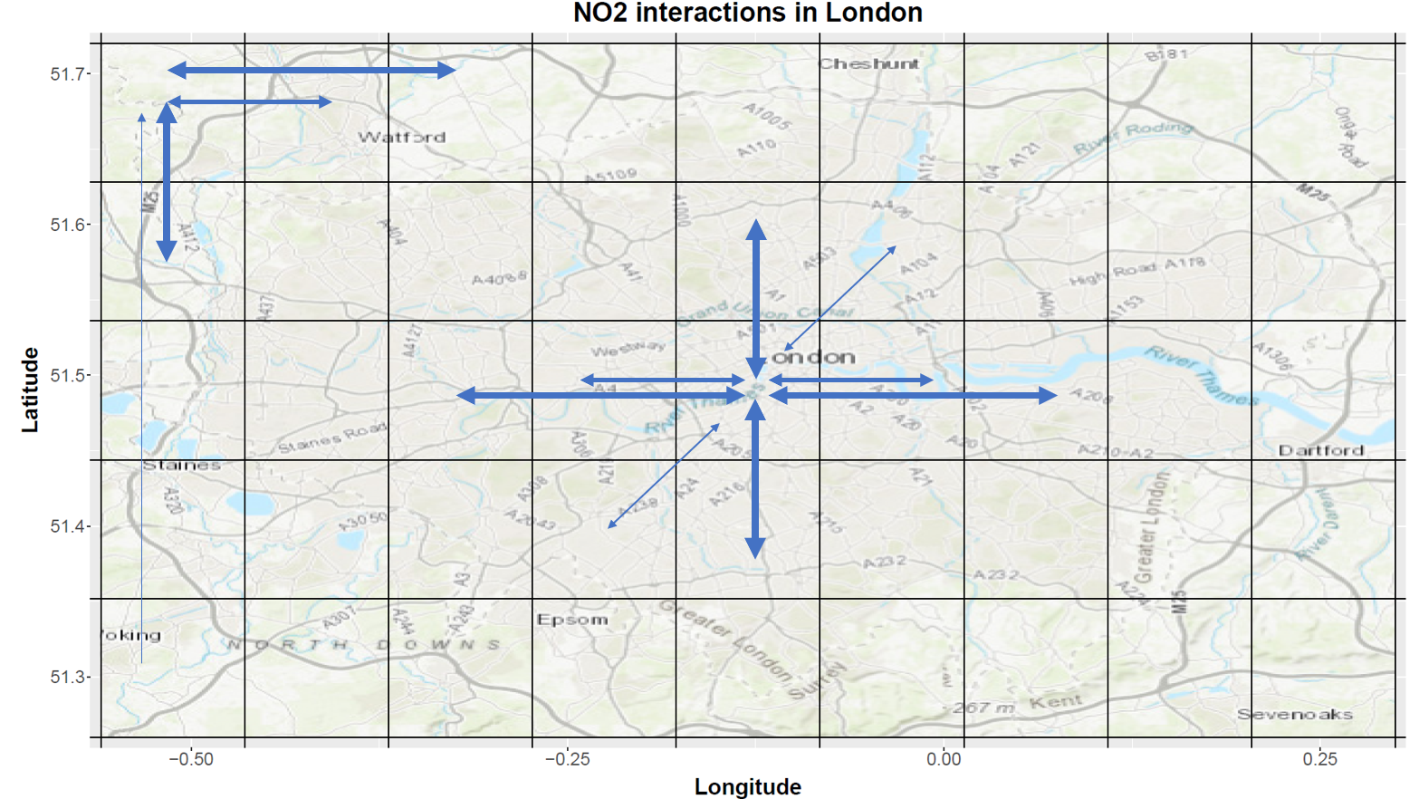
Nitrogen dioxide (NO2) is emitted during combustion of fossil fuels (e.g. by motor vehicles) and it has been associated with adverse effects on the respiratory system.1111 11 The direct health effect of nitrogen dioxide is difficult to determine because its emission process is typically accompanied with the emission of other air pollutants (see, e.g. Brunekreef and Holgate, 2002). The Air Quality Standards Regulations 2010 requires a regular monitoring of NO2 concentration levels in the UK.1212 12 Source: https://www.legislation.gov.uk/uksi/2010/1001/contents/made. Using satellite data, we examine the empirical performance of the SPLASH estimator when predicting daily NO2 concentrations in Greater London. This satellite data is publicly available via the Copernicus Open Access Hub and we consider the time span from 1 August 2018 to 18 October 2020.1313 13 See http://www.tropomi.eu/ for more info on TROPOMI data products and use https://scihub.copernicus.eu/ to access the database. The original concentrations are reported in mol/m2, which we convert to mol/cm2 to avoid numerical instabilities caused by small-scale numbers. The far majority of measurements are captured between 11:00 and 14:00 UTC. The area of interest is divided into a () grid, implying that longitudes and latitudes increment by approximately 0.2 from cell to cell (see Figure 4, part c). All available measurements are averaged within each cell and within the same day. The resulting data set contains 0.8% missing observations, which we impute using the Multivariate Time Series Data Imputation (mtsdi) R package.1414 14 This imputation method is proposed by Junger and Ponce De Leon, 2015 to impute missing values in time series for air pollutants. The package is written by the same authors and currently maintained by W. L. Junger.
A rolling-window approach is used to assess the predictive power of the SPLASH estimator. Each window contains 80% of the data (641 days) allowing 160 one-step ahead forecasts to be made. For each window, we proceed along the following four steps: (i) de-mean the data, (ii) determine the hyperparameters and estimate each model, (iii) produce a forecast for the de-meaned data, and (iv) add the means back to the forecast. In addition to the estimators described in the simulation section (Section 4, see page 4), we add another forecast: the window’s mean. This new forecast is abbreviated CONST and all other forecasts follow the notational conventions from the simulation section. For SPLASH, we follow the procedure described in Section 4.1 and set . The spatial grid contains spatial units, such that the SPLASH(,) models contain parameters. For the purpose of identifiability, we band the spatial matrix and autoregressive matrix such that for . By ordering the spatial units vertically, this banding puts no restrictions on the vertical interactions but allows no more than second-order interaction between horizontal neighbours (see Figure in the Supplementary Appendix for details).
The forecast performance is measured along three metrics and is always expressed relative to the -penalized reduced form VAR() (PVAR) benchmark. That is, we report: (i) the number of spatial units that are predicted more accurately than the PVAR method (#wins), (ii) the number of spatial units that are predicted significantly more accurately based on a Diebold-Mariano test at a 5% significance level (#sign. wins), and (iii) the average loss relative to the penalized VAR over all spatial units. These three metrics are calculated based on two loss functions for the forecast errors, namely the mean squared forecast error (MSFE) and the mean absolute forecast error (MAFE). We additionally report the MAFE because the column densities display several abrupt spikes which may carry too much weight when relying on a squared loss function. The results are reported in Table 5.
| MSFE | MAFE | ||||||
|---|---|---|---|---|---|---|---|
| #wins | #sign. wins | RMSFE | #wins | #sign. wins | RMAFE | ||
| CONST | 0 | 0 | 1.187 | 0 | 0 | 1.139 | |
| GMWY | 0 | 0 | 153.393 | 0 | 0 | 4.855 | |
| SPLASH(,) | 45 | 42 | 0.919 | 45 | 44 | 0.941 | |
| SPLASH(,) | 44 | 39 | 0.931 | 45 | 42 | 0.949 | |
| SPLASH(,) | 44 | 30 | 0.940 | 45 | 35 | 0.957 | |
- •
Note: Number of grid points (out of ) with lower prediction errors (#wins) and significantly lower prediction errors (#sign.) compared to the -penalized reduced form VAR() estimator (PVAR). Relative MAFE and MSFE are abbreviated by RMAFE and RMSFE, respectively. Values below (above) 1 indicate superior (inferior) performance compared to PVAR.
We first look at the mean squared forecast errors (MSFEs). The window-mean forecast (CONST) clearly does not improve the benchmark PVAR forecast for any spatial unit. However, this forecast still attains a RMSFE of 1.185, potentially indicating a low predictability of column densities. The GMWY approach obtains the worst forecast performance, possibly because a large bandwidth is needed to allow for second-order horizontal interaction and, consequently, a large number of parameters to estimate. With an RMSFE of 0.919, SPLASH(0,) does manage to improve upon the benchmark. In fact, the MSFEs for all 45 spatial units are smaller than that of the benchmark, 42 of which are found to be significant by a Diebold-Mariano test based on the squared forecast errors. Allowing for sparsity within groups does not seem to deliver additional forecast improvements, as SPLASH(0.5,) attains a slightly worse forecast performance and significantly outperforms the benchmark for only 39 locations. Completely omitting regularization at the group level results in a further deterioration of the forecast performance, with SPLASH(1,) attaining an RMSFE of 0.94 and significantly beating the benchmark for 30 out 45 spatial units. We take this as evidence that the ability to promote diagonally structured sparsity is indeed beneficial in real-life spatial applications, although even estimating the spatial VAR with unstructured sparsity manages to improve upon regularized reduced form VAR estimation.
Next, we focus on the mean absolute forecast error (MAFE). The results are qualitatively similar to those obtained based on the MSFE. In particular, GMWY still has the worst forecast accuracy for GMWY and SPLASH(0,) continues to perform best. The GMWY method, while still standing out, does not score as poorly anymore based on the RMAFE. We conjecture that the absence of regularization may increase sensitivity to noise, thereby resulting in particularly high squared forecast errors at periods of atypical NO2 concentrations.
Finally, we illustrate the second key benefit of SPLASH-type estimators: interpretability. Recall that we convoluted satellite images to a () grid of spatial units. To examine the relevant interactions between these spatial units, we provide several visualizations off the spatial weight matrices estimated by the SPLASH(0.5,) estimator. First, in Figure 4(a), we visualize the absolute magnitude of the spatial interactions. A clear diagonal pattern emerges, with the two diagonals closest to the principal diagonal and the two outer diagonals containing the largest interactions. These four diagonals correspond to first-order vertical and second-order horizontal interactions, respectively. The additional two diagonals, that are sandwiched in between the former, contain the first-order horizontal interactions between spatial units, which surprisingly seem to be smaller in magnitude. In Figure 4(b), each cell indicates the proportion of rolling windows the corresponding spatial interaction is estimated as being non-zero. These proportions are either one (yellow) or zero (purple) indicating very stable selection across samples. It becomes apparent that in addition to the six diagonals that were clear from panel (a), two additional diagonals are always selected, which contain the first order diagonal interactions between spatial units. To facilitate interpretation of this sparsity pattern, we provide a spatial plot of our region of interest with the spatial grid overlaid (Figure 4(c)). We explicitly visualize the interactions implied by 4(b) for two pixels – pixel 1 (left-top) and pixel 23 (center) – using arrows whose thickness is determined by the average absolute magnitudes estimated in Figure 4(a). The emerging pattern of spatial interactions shows clearly the interactions between NO2 concentrations of neighbouring districts in London. The wider horizontal interactions, as well as the diagonal interactions, may be explainable by the “prevailing winds”, which come from the West or South-West and are the most commonly occurring winds in London. Overall, the intuitive sparsity patterns that arise, in combination with the improvement in forecast performance, are encouraging and provide empirical validation for the use of SPLASH on spatial data, especially when the spatial units follow a natural ordering on a spatial grid.
6 Conclusion
In this paper, we develop the Spatial Lasso-type Shrinkage (SPLASH) estimator, a novel estimation procedure for high-dimensional spatio-temporal models. The SPLASH estimator is designed to promote the recovery of structured forms of sparsity without imposing such structure a priori. We derive consistency of our estimator in a joint asymptotic framework in which the number of both spatial units and temporal observations diverge. To solve the identifiability issue, we rely on a relatively non-restrictive assumption that the coefficient matrices in the spatio-temporal model are sufficiently banded. Based on this assumption, we consider banded estimation of high-dimensional spatio-temporal autocovariance matrices, for which we derive novel convergence rates that are likely to be of independent interest. The SPLASHX extension explains how to include exogenous variables. As an application, we use SPLASH to predict satellite-measured NO2 concentrations in London. We find evidence for spatial interactions between neighbouring regions. In addition, our estimator obtains superior forecast accuracy compared to a number of competitive benchmarks, including the recently introduced spatio-temporal estimator by Gao et al., 2019 (the inspiration for the development of SPLASH).
7 Acknowledgements
This paper (or earlier versions hereof) has been presented during the internal seminar of the Quantitative Economics department of Maastricht University, the Econometrics Internal Seminar (EIS) at Erasmus University Rotterdam, the Bernoulli-IMS One World Symposium, the workshop on Dimensionality Reduction and Inference in High-dimensional Time Series at Maastricht University, the 2021 Annual Conference of the International Association for Applied Econometrics (IAAE), the 5th Conference on Econometric Models of Climate Change, the internal seminar at Tor Vergata University of Rome, and the 2021 Conference. We gratefully acknowledge comments and feedback from the participants. Suggestions by Stephan Smeekes and Ines Wilms were particularly helpful so we thank them explicitly. All remaining errors are our own.
References
- Ahrens and Bhattacharjee, (2015) Ahrens, A. and Bhattacharjee, A. (2015). Two-step lasso estimation of the spatial weights matrix. Econometrics, 3:128–155.
- Bickel et al., (2009) Bickel, P. J., Ritov, Y., and Tsybakov, A. B. (2009). Simultaneous analysis of lasso and Dantzig selector. The Annals of Statistics, 37:1705–1732.
- Brockwell and Davis, (1991) Brockwell, P. J. and Davis, R. A. (1991). Time Series: Theory and Methods. Springer-Verlag, New York, 2nd edition.
- Brunekreef and Holgate, (2002) Brunekreef, B. and Holgate, S. T. (2002). Air pollution and health. The Lancet, 360(9341):1233–1242.
- Debarsy and LeSage, (2018) Debarsy, N. and LeSage, J. (2018). Flexible dependence modeling using convex combinations of different types of connectivity structures. Regional Science and Urban Economics, 69:48–68.
- Dou et al., (2016) Dou, B., Parrell, M. L., and Yao, Q. (2016). Generalized Yule-Walker estimation for spatio-temporal models with unknown diagonal coefficients. Journal of Econometrics, 194:369–382.
- Gao et al., (2019) Gao, Z., Ma, Y., Wang, H., and Yao, Q. (2019). Banded spatio-temporal autoregressions. Journal of Econometrics, 208:211–230.
- Gelper et al., (2016) Gelper, S., Wilms, I., and Croux, C. (2016). Identifying demand effects in a large network of product categories. Journal of Retailing, 92:25–39.
- Guo et al., (2016) Guo, S., Wang, Y., and Yao, Q. (2016). High-dimensional and banded vector autoregressions. Biometrika, 103:889–903.
- Hyndman and Athanasopoulos, (2018) Hyndman, R. J. and Athanasopoulos, G. (2018). Forecasting: principles and practice. OTexts.
- Jing et al., (2003) Jing, B.-Y., Shao, Q.-M., and Wang, Q. (2003). Self-normalized Cramér-type large deviations for independent random variables. Annals of Probability, 31:2167–2215.
- Junger and Ponce De Leon, (2015) Junger, W. L. and Ponce De Leon, A. (2015). Imputation of missing data in time series for air pollutants. Atmospheric Environment, 102:96–104.
- Kock and Callot, (2015) Kock, A. B. and Callot, L. (2015). Oracle inequalities for high dimensional vector autoregressions. Journal of Econometrics, 186:325–344.
- Lam and Souza, (2014) Lam, C. and Souza, P. C. L. (2014). Regularization for spatial panel time series using the adaptive lasso. Working paper, London School of Economics and Political Science.
- Lam and Souza, (2019) Lam, C. and Souza, P. C. L. (2019). Estimation and selection of spatial weight matrix in a spatial lag model. Journal of Business & Economic Statistics, 38:1–41.
- Lee, (2004) Lee, L.-F. (2004). Asymptotic distributions of quasi-maximum likelihood estimators for spatial autoregressive models. Econometrica, 72:1899–1925.
- Lee and Yu, (2010) Lee, L.-F. and Yu, J. (2010). Estimation of spatial autoregressive panel data models with fixed effects. Journal of Econometrics, 154:165–185.
- Lee and Yu, (2014) Lee, L.-f. and Yu, J. (2014). Efficient GMM estimation of spatial dynamic panel data models with fixed effects. Journal of Econometrics, 180:174–197.
- Ma et al., (2021) Ma, Y., Guo, S., and Wang, H. (2021). Sparse spatio-temporal autoregressions by profiling and bagging. Journal of Econometrics, X:XX–XX.
- Masini et al., (2019) Masini, R. P., Medeiros, M. C., and Mendes, E. F. (2019). Regularized estimation of high-dimensional vector autoregressions with weakly dependent innovations. Journal of Time Series Analysis.
- Medeiros and Mendes, (2016) Medeiros, M. C. and Mendes, E. F. (2016). -regularization of high-dimensional time series models with non-gaussian and heteroskedastic errors. Journal of Econometrics, 191:255–271.
- Simon et al., (2013) Simon, N., Friedman, J., Hastie, T., and Tibshirani, R. (2013). A sparse-group lasso. Journal of Computational and Graphical Statistics, 22:231–245.
- Yu et al., (2012) Yu, J., de Jong, R., and Lee, L.-f. (2012). Estimation for spatial dynamic panel data with fixed effects: The case of spatial cointegration. Journal of Econometrics, 167:16–37.
- Yu et al., (2008) Yu, J., de Jong, R. M., and Lee, L.-F. (2008). Quasi-maximum likelihood estimators for spatial dynamic panel data with fixed effects when both n and T are large. Journal of Econometrics, 146:118–134.
- Zhang and Yu, (2018) Zhang, X. and Yu, J. (2018). Spatial weight matrix selection and model averaging for spatial autoregressive models. Journal of Econometrics, 203:1–18.
Appendix A Lemmas
Lemma 1.
Proof.
First, we show that (16) is bounded from below by 0.5 times the smallest singular value of . For , it holds that
Alternatively, for , we have . Combining the two previous results yields
| (17) |
for any .
Lemma 2.
Define the set . Then, under Assumption 4, it holds on that
Proof.
First, recall the construction of with containing at most columns of the matrix . From the block-diagonal construction, it follows that
Then,
| (18) |
where the last inequality follows holds on the set . Consequently,
where (i) follows from the proof of Lemma 1, (ii) holds by (18), and (iii) from Lemma 1. ∎
Appendix B Proofs of Main Results
Proof of Theorem 1.
We first prove various intermediate results, see (a)–(d) below. We afterwards combine these results and recover Theorem 1.
- (a)
The matrix has a maximum bandwidth of and satisfies
- (b)
Define with as in Theorem 1(a). The matrix is a banded matrix with bandwidth no larger than . Moreover,
whenever is large enough such that .
- (c)
- (d)
Take any , then
with a probability of at least (for polynomial tail decay) or (for exponential tail decay).
- (e)
Take any , then
with a probability of at least (for polynomial tail decay) or (for exponential tail decay).
Explicit expressions for , , , and are provided in the proofs below.
(a) The proof builds upon results from Guo et al., 2016 on banded vector autoregressions. Recall that with . has a bandwidth of at most and satisfies1515 15 If matrices and are banded matrices with bandwidths and , respectively, then the product is again a banded matrix with a bandwidth of at most .
The product has a maximal bandwidth of . Since (Assumption 3(c)), we also have
and the claim follows with . (b) Iterating on the observation in footnote 15, we conclude that the bandwidth of is at most . The bandwidth of therefore does not exceed
We now bound . Assumption 1(b), imposes for some . Because , it holds that
| (19) | ||||
An inspection of (19) shows that additional upper bounds are required on , , and . For , using properties of matrix norms and Theorem 1(a), we obtain
| (20) |
Furthermore, expanding the matrix powers provides
| (21) | ||||
Finally, since and (Assumption 1(a)), we have
| (22) |
Returning to (19) and inserting the upper bounds in (20)–(22), we find
Assuming is sufficient large, that is assuming , we subsequently use result on geometric series and conclude1616 16 Specifically, and for .
The claim is thus indeed valid with . (c) We have , and hence
| (23) |
Now combine (since is taken sufficiently large), Theorem 1(b), (21) with , and to obtain the stated result with . (d) We have
| (24) | ||||
because is a banded matrix already and banding can only decrease the norm difference between and . We consider the three terms in the RHS of (24) separately. There are at most nonzero elements in any column/row of and thus
| (25) |
and
| (26) | ||||
where the last inequality exploits Lemma (see Supplement). Note that the probabilities in (26) coincide with the probabilities defined as and in Theorem 1. Overall, if holds, then continuing from (24),
where the last inequality follows from part (b) of this proof. A lower bound on the probability of occurring is immediately available from (26).
(e) Mimicking the steps from (d), we find
if we use part (c) and if holds. The probability of the latter event is (polynomial tails) or (exponential tails).
We now combine all these intermediate results to recover the result from the theorem. Parts (d) and (e) are both applicable since
Lemma implies that
when takes place and . From it follows that this joint event takes place with probabilities and in the cases of polynomial and exponential tail decay, respectively.
It remains to determine and such that and hold. For any with , we have . Under the latter assumption, we determine the such that
Similarly, for , the choice suffices. ∎
Proof of Theorem 2.
The proof of the theorem relies on the properties of dual norms. Recall . Exploiting the properties of and , it is straightforward to verify that is a norm for any . For any norm , we define its dual norm through . The dual-norm inequality states that
| (27) |
For the norm , its dual norm is bounded by
| (28) | ||||
by convexity of the function in step (i), and using for step (ii) both and
We now start the actual proof. Recall , , , and . Exploiting standard properties of , we find
| (29) | ||||
Using (29), we rewrite
Recalling the objective function and noting that by construction, it follows that
| (30) | ||||
where we used the dual-norm inequality (see (27)) and the triangle property of (dual) norms in the second and third inequality, respectively. Define the sets
| (31) |
On the set , we can scale (30) by a factor 2 to obtain
| (32) |
We subsequently manipulate and . Using the reverse triangle inequality, we have
| (33) | ||||
where and are defined in Lemma 1. Simple rewriting provides
| (34) | ||||
Combining results (32)–(34) yields
| (35) |
and is thus a member of the set as defined in Lemma 1.
In combination with Lemma 2, thus requiring to hold, we conclude
| (36) | ||||
where step (i) follows from (35), step (ii) is implied by for (Lemma 2), and step (iii) uses the elementary inequality (i.e. manipulating ). A straightforward rearrangement of (36) provides the inequality of Theorem 2.
It remains to determine a lower bound on the probability of . We rely on the elementary inequality to bound the individual probabilities.
We start with . The last inequality is true because continuing from (28), we have
| (37) |
for any vector . Subsequently, we have
| (38) | ||||
exploiting block-diagonality of and such that and (explicitly assumed in Theorem 2). Bounds for the final RHS terms in (38) are available from Theorem 1.
Second, we have
| (39) | ||||
where the last line relies on the union bound and the fact that (implied by Assumption 1). Hence, the sets and admit the same probability bound.
Proof of Corollary 1.
First, we derive the conditions under which the set on which the performance bound in Theorem 2 holds occurs with probability converging to one. Under Assumption 2(b1), along with the remaining assumptions in Theorem 2, this probability is given by , where we recall from Theorem 1 that
| (41) |
Given that with , it follows immediately that
| (42) |
In addition, following the remark below Theorem 1, it holds that
| (43) |
Based on (42) and (43), it follows that the first RHS-term in (41) converges to zero exponentially in for any . The second RHS-term, however, converges to zero at most at a polynomial rate. Accordingly,
| (44) |
where the second equality holds from the observation that for any the first two RHS terms in the first equality converge to zero at an exponential rate, whereas the third term may converge to zero at most at a polynomial rate. From (44), it follows that if
In a similar fashion, we derive the conditions under which , by noting that
| (45) |
converges to zero exponentially fast in if diverges at a polynomial rate in . Making use of (42) and (43), it follows that
which translates to the condition , or . This establishes conditions (i) and (ii) in Corollary 1.
We proceed by deriving the order of the performance bound in Theorem 2. Noting that
it follows that
Then, by Theorem 2,
and
on a set with probability or , depending on whether Assumption 2(b1) or 2(b2) applies, respectively. Since we have shown that both and under the conditions imposed in Corollary 1, the proof is complete. ∎