跳到论文正文
W Papers独立论文阅读器 arXiv:2108.02857 论文正文 计算阅读时间 · 0%
引用这篇论文根据当前论文元数据生成,正式投稿前建议核对。


License: CC Zero
arXiv:2108.02857v1 [math.PR] 05 Aug 2021

Asymptotics of Yule’s nonsense correlation for Ornstein-Uhlenbeck paths: a Wiener chaos approach.

Soukaina Douissi Thanks: National School of Applied Sciences, Marrakech, Morocco. Email:s.douissi@uca.ma    Frederi Viens Thanks: Department of Statistics and Probability, Michigan State University, USA. E-mail: viens@msu.edu    Khalifa Es-Sebaiy Thanks: Department of Mathematics, Faculty of Science, Kuwait University, Kuwait. E-mail: khalifa.essebaiy@ku.edu.kw
August 11, 2026
Abstract

In this paper, we study the distribution of the so-called "Yule’s nonsense correlation statistic" on a time interval [0,T][0,T] for a time horizon T>0T>0 , when TT is large, for a pair (X1,X2)(X_{1},X_{2}) of independent Ornstein-Uhlenbeck processes. This statistic is by definition equal to :

ρ⁡(T):=Y12​(T)Y11​(T)​Y22​(T),\rho(T):=\frac{Y_{12}(T)}{\sqrt{Y_{11}(T)}\sqrt{Y_{22}(T)}},

where the random variables Yi​j​(T)Y_{ij}(T), i,j=1,2i,j=1,2 are defined as

Yi​j(T):=∫0TXi(u)Xj(u)du−TX¯iXj¯,  X¯i:=1T∫0TXi(u)du.Y_{ij}(T):=\int_{0}^{T}X_{i}(u)X_{j}(u)du-T\bar{X}_{i}\bar{X_{j}},\text{ \ }\text{ \ }\bar{X}_{i}:=\frac{1}{T}\int_{0}^{T}X_{i}(u)du.

We assume X1X_{1} and X2X_{2} have the same drift parameter θ>0\theta>0. We also study the asymptotic law of a discrete-type version of ρ⁡(T)\rho(T), where Yi​j​(T)Y_{ij}(T) above are replaced by their Riemann-sum discretizations. In this case, conditions are provided for how the discretization (in-fill) step relates to the long horizon TT. We establish identical normal asymptotics for standardized ρ⁡(T)\rho(T) and its discrete-data version. The asymptotic variance of ρ⁡(T)​T1/2\rho(T)T^{1/2} is θ−1\theta^{-1}. We also establish speeds of convergence in the Kolmogorov distance, which are of Berry-Esséen-type (constant*T−1/2T^{-1/2}) except for a ln⁡T\ln T factor. Our method is to use the properties of Wiener-chaos variables, since ρ⁡(T)\rho(T) and its discrete version are comprised of ratios involving three such variables in the 2nd Wiener chaos. This methodology accesses the Kolmogorov distance thanks to a relation which stems from the connection between the Malliavin calculus and Stein’s method on Wiener space.

1 Introduction

In this paper, we study the normal asymptotics in law of the so-called “Yule’s nonsense correlation statistic” on a time interval [0,T][0,T] when the time horizon T>0T>0 tends to infinity, for two independent paths of the Ornstein-Uhlenbeck (OU) stochastic processes. This statistic is defined as:

ρ⁡(T):=Y12​(T)Y11​(T)​Y22​(T),\rho(T):=\frac{Y_{12}(T)}{\sqrt{Y_{11}(T)}\sqrt{Y_{22}(T)}}, (1)

where the random variables Yi​j​(T)Y_{ij}(T), i,j=1,2i,j=1,2 are given by

Yi​j(T):=∫0TXi(u)Xj(u)du−TX¯i(T)Xj¯(T),  X¯i(T):=1T∫0TXi(u)du,Y_{ij}(T):=\int_{0}^{T}X_{i}(u)X_{j}(u)du-T\bar{X}_{i}\left(T\right)\bar{X_{j}}\left(T\right),\text{ \ }\text{ \ }\bar{X}_{i}\left(T\right):=\frac{1}{T}\int_{0}^{T}X_{i}(u)du, (2)

and (X1,X2)(X_{1},X_{2}) is a pair of two independent OU processes with the same known drift parameter θ>0\theta>0, namely XiX_{i} solves the linear SDE, for i=1,2i=1,2

dXi(t)=−θXi(t)dt+dWi(t), t⩾0dX_{i}(t)=-\theta X_{i}(t)dt+dW^{i}(t),\text{ \ }t\geqslant 0 (3)

with Xi​(0)=0X_{i}(0)=0, i=1,2i=1,2, where the driving noises (W1​(t))t⩾0(W^{1}(t))_{t\geqslant 0}, (W2​(t))t⩾0(W^{2}(t))_{t\geqslant 0} are two independent standard Brownian motions (Wiener processes). We also study the asymptotic law of a discrete-data version of ρ⁡(T)\rho(T), denote by ρ~​(n)\tilde{\rho}(n) for nn observations, where the Riemann integrals in (2) are replaced by Riemann-sum approximations.

It has been known since 1926 that a discrete version of the statistic ρ\rho, which is the Pearson correlation coefficient, does not behave the same way when the data from X1X_{1} and X2X_{2} are i.i.d. and as when they are the discrete-time observations of a random walk. As is universally known for i.i.d. data, and also holds for shorter-memory models, ρ~​(n)\tilde{\rho}(n) converges in probability to 00 under all but the most extreme circumstances (data coming from a distribution with no second moment), but G. Udny Yule showed in [12] that when the data come from a random walk, ρ~​(n)\tilde{\rho}(n) does not concentrate, and has a law which seems to converge instead to a diffuse distribution on (−1,1)(-1,1). The exact variance and other statistical properties of this law remained unknown with mathematical precision, though a 1986 paper [5] by P.C.B. Phillips showed that the limiting law of ρ~​(n)\tilde{\rho}(n) with simple symmetric random-walk data rescaled to the time interval [0,1][0,1] is the same as the law of ρ⁡(1)\rho(1) for two independent Wiener processes, which is indeed necessarily diffuse and fully supported on (−1,1)(-1,1). This advance prompted several talented prominent probabilists to look for ways of computing statistics of ρ⁡(1)\rho(1), if even only its variance, but this remained elusive until 2017, when Ph. Ernst and two collaborators (one posthumous) provided a closed-form expression for V​a​r​[ρ⁡(1)]Var[\rho(1)] in [1]. Since then, other advances on the moments of ρ⁡(1)\rho(1) have been made, particularly [2], and recent progress was recorded in [3] on how to compute the momens of ρ~​(n)\tilde{\rho}(n) when the paths (X1,X2)(X_{1},X_{2}) are independent Gaussian simple-symmetric random walks. In all cases mentioned in this paragraph, the asymptotic behavior of ρ~​(n)\tilde{\rho}(n) in law (scaled appropriately in time) is necessarily that of ρ⁡(1)\rho(1) for two independent Wiener processes.

This leaves open the question of what happens to ρ~​(n)\tilde{\rho}(n) when the paths (X1,X2)(X_{1},X_{2}) deviate substantially from Wiener paths or random walks. Wiener (resp. random walk) paths have the property of exact (resp. approximate) self-similarily. We take up the question of using different kinds of paths, with the simplest possible example of a clear alternative to self-similar processes, namely the ubiquitous mean-reverting OU processes. The property of mean reversion is so distinct from self-similarily, that the behavior of ρ⁡(T)\rho(T) changes drastically from one to the other. Note that these two classes of processes are simply those satisfying (3) with θ=0\theta=0 (Wiener process) or θ≠0\theta\neq 0 (OU process). To illustrate the point of how distinct these processes are, let us extend the scope of this paper momentarily, to include all processes defined by (3) (with or without θ=0\theta=0), by replacing WW with a fractional Brownian motion (fBm) denoted by BHB^{H}, for some H∈(0,1)H\in(0,1). Like the Wiener process, which corresponds to H=1/2H=1/2, the self-similar property of BHB^{H} simply states that for any fixed real constant aa, BH(a⋅)=aHBH(⋅)B^{H}(a\cdot)=a^{H}B^{H}\left(\cdot\right) in law. By using this property with a=Ta=T via the change of variable u′=u/Tu^{\prime}=u/T in the Riemann integrals defining ρ⁡(T)\rho(T), we obtain immediately the equality in law

Yi​j​(T)\displaystyle Y_{ij}\left(T\right) =\displaystyle= ∫01TH​Xi​(u′)​TH​Xj​(u′)​T​d​u′−T−1​TH+1​X¯i​(1)​TH+1​Xj¯​(1)\displaystyle\int_{0}^{1}T^{H}X_{i}(u^{\prime})T^{H}X_{j}(u^{\prime})Tdu^{\prime}-T^{-1}T^{H+1}\bar{X}_{i}\left(1\right)T^{H+1}\bar{X_{j}}\left(1\right)
=\displaystyle= T2​H+1​Yi​j​(1)\displaystyle T^{2H+1}Y_{ij}\left(1\right)

and therefore

ℒ⁡(ρ⁡(T))=ℒ⁡(ρ⁡(1)).\mathcal{L}\left(\rho\left(T\right)\right)=\mathcal{L}\left(\rho\left(1\right)\right).

In fact, we only used the property of self-similarity to get the above. In other words, for any pair of self-similar processes, the law of the nonsense correlation ρ⁡(T)\rho\left(T\right) is constant as the time horizon TT increases. In stark contrast, in this paper, we show that, for a pair of OU processes, the law of ρ⁡(T)\rho\left(T\right) converges to the Dirac mass at 0. As mentioned, we show more: a central limit theorem for ρ⁡(T)​T\rho\left(T\right)\sqrt{T} (the mean of ρ⁡(T)\rho\left(T\right) is always 0), with asymptotic variance equal to θ−1\theta^{-1}, and a speed of convergence of ℒ⁡(ρ⁡(T)​T1/2)\mathcal{L}\left(\rho\left(T\right)T^{1/2}\right) to N⁡(0,θ−1)N\left(0,\theta^{-1}\right) in Kolmogorov metric at the rate T−1/2lnTT^{-1/2}\ln T.

The discrete-observation part of this paper simply replaces the Riemann integrals by the Riemann sums, for instance replacing the first integral in Yi​j​(T)Y_{ij}\left(T\right) by Δn​∑k=0n−1Xi​(tk)​Xj​(tk)\Delta_{n}\sum\limits_{k=0}^{n-1}X_{i}(t_{k})X_{j}(t_{k}) where Δn=T/n\Delta_{n}=T/n and tk=k​T/nt_{k}=kT/n. We denote the resulting empirical correlation by ρ~​(n)\tilde{\rho}(n) rather than ρ⁡(T)\rho(T). It is convenient to note that T=n​ΔnT=n\Delta_{n} can be thought of as depending on nn, and we will systematically emphasize this by denoting T=TnT=T_{n}. It is assumed that the discretization step Δn\Delta_{n} converges to 00 while Tn=TT_{n}=T tends to ∞\infty, which means that n≫Tnn\gg T_{n} in our asymptotics. We provide a full range of speeds of convergence in central limit theorem depending on how fast Δn\Delta_{n} converges to 0.0. We find in fact that we must have Tn​Δn=n​Δn2→0T_{n}\Delta_{n}=n\Delta_{n}^{2}\rightarrow 0 as n→∞,n\rightarrow\infty, and we also note that n​Δn=Tn=T→∞n\Delta_{n}=T_{n}=T\rightarrow\infty, as well it should. Our convergence result, which immediately implies the central limit theorem limn→∞ℒ⁡(ρ~​(n)​Tn1/2)=𝒩⁡(0,θ−1)\lim_{n\rightarrow\infty}\mathcal{L}\left(\tilde{\rho}(n)T_{n}^{1/2}\right)=\mathcal{N}\left(0,\theta^{-1}\right), is

dK​o​l​(θ​Tn​ρ~​(n),𝒩⁡(0,1))\displaystyle d_{Kol}\left(\sqrt{\theta}\sqrt{T_{n}}\tilde{\rho}(n),\mathcal{N}(0,1)\right) ⩽\displaystyle\leqslant c(θ)×ln(nΔn)max((nΔn)−1/2,(nΔn2)13)\displaystyle c(\theta)\times\ln(n\Delta_{n})\max\left((n\Delta_{n})^{-1/2},(n\Delta_{n}^{2})^{\frac{1}{3}}\right)
=\displaystyle= c(θ)×ln(Tn)max(Tn−1/2,(TnΔn)13).\displaystyle c(\theta)\times\ln(T_{n})\max\left(T_{n}^{-1/2},(T_{n}\Delta_{n})^{\frac{1}{3}}\right).

From this, we can immediately read off that a rather optimal rate of sampling of our discrete data is one for which the two terms in the max are of the same order, i.e. Tn−1/2≍(TnΔn)13T_{n}^{-1/2}\asymp(T_{n}\Delta_{n})^{\frac{1}{3}}, which is equivalent to requiring that Δn\Delta_{n} be of order Tn−5/2T_{n}^{-5/2}, which in turn, since Tn=n​ΔnT_{n}=n\Delta_{n}, is equivalent to Δn\Delta_{n} of order n−5/7n^{-5/7}. This is explained in more detail in the conclusion of the section on discrete data. In any case, in Kolmogorov distance, we see that the best rate of convergence of Tn​ρ~​(n)\sqrt{T_{n}}\tilde{\rho}(n) to N⁡(0,θ−1)N\left(0,\theta^{-1}\right) is of order Tn−1/2lnTnT_{n}^{-1/2}\ln T_{n}, which is exactly the same rate as in the case of continuous data, and which occurs for a relatively frequency of observations of order Δn−1=Tn5/2\Delta_{n}^{-1}=T_{n}^{5/2} over unit intervals. Lower frequency of observations lead to slower convergence rate in Kolmogorov distance in the scale of the time horizon TnT_{n} compared to continuous observation. Higher frequency of observation leads to the same rate Tn−1/2lnTnT_{n}^{-1/2}\ln T_{n} as with continuous observations, but this can be considered wasteful since the same rate was achieved at the optimal frequency of Δn−1=Tn5/2\Delta_{n}^{-1}=T_{n}^{5/2} per unit time. It is worth stating again that these results in discrete time, pertaining to the convergence rate in the CLT for Tn​ρ~​(n)\sqrt{T_{n}}\tilde{\rho}(n), are a second-order result compared to the CLT itself, i.e.

limn→∞Tn​ρ~​(n)=limT→∞T​ρ​(T)=𝒩⁡(0,θ−1)\lim_{n\rightarrow\infty}\sqrt{T_{n}}\tilde{\rho}(n)=\lim_{T\rightarrow\infty}\sqrt{T}\rho(T)=\mathcal{N}(0,\theta^{-1})

which holds in law identically in both the discrete and continuous data cases.

As mentioned, we use techniques from analysis on Wiener chaos to prove the above results. Some of these results are technical and novel, and we provide here a few points in the hopes of enlightening the methods. A key element comes from the connection discovered by I. Nourdin and G. Peccati (see [8]) between the Malliavin calculus and Stein’s method. In that connection, the distance in law between a random variable XX and the standard normal law can be measured to some extent by comparing the Hilbert-space norm of the Malliavin derivative D​XDX to the value 11, which is the value one would find for the norm of the Malliavin derivative of a standard normal variable NN under any reasonable coupling of XX and N,N, i.e. under any reasonable representation of XX on Wiener space. The question of how to represent XX on Wiener space is typically trivial when dealing with functionals of stochastic processes based on Wiener processes, and this is certainly the case in our paper. The question of whether D​XDX is an adeqate functional of XX to make the comparison with 𝒩⁡(0,1)\mathcal{N}\left(0,1\right) is less trivial. The original work in [4] noted that it is sufficient for variables on Wiener chaos, and used an auxiliary random variable GXG_{X} which is slightly more involved than ‖D​X‖2\left\|DX\right\|^{2} to establish broader convergence in law beyond fixed chaos. That same random variable GXG_{X} was used in [9] to characterize laws on Wiener chaos at the level of densities, and was used specifically in [6, Theorem 2.4] to measure distances between laws in the Kolmogorov metric. We use that theorem herein, by applying it separately to all three Wiener chaos components Y11,​Y22,Y12Y_{11,}Y_{22},Y_{12} which are used to calculate ρ⁡(T)\rho\left(T\right), noting as in [4] that GX=2​‖D​X‖2G_{X}=2\left\|DX\right\|^{2}.

The above elements are explained in the preliminary section on analysis on Wiener space below. They are used herein via standard computations of variances and differentiation and product rules for variables on Wiener chaos which are represented as double Wiener integrals with respect to the WiW_{i}’s, leading to computing the asymptotic variance of the rescaled numerator T−1/2Y12(T)T^{-1/2}Y_{12}(T), namely 1/4​θ31/4\theta^{3}, and the speed of convergence of the variances to this limit, including precise estimations of the constants in this rate of convergence as functions of θ\theta. It turns out that the rescaled denominator T−1​(Y11​(T)​Y22​(T))1/2T^{-1}(Y_{11}\left(T\right)Y_{22}\left(T\right))^{1/2} does not have normal fluctuations, but rather converges to the constant 1/2​θ1/2\theta. We establish this too. Adding to this that the numerator, as a second-chaos variable, has mean zero, this indicates that the entire rescaled fraction ρ\rho should converge in law to 𝒩⁡(0,θ−1).\mathcal{N}\left(0,\theta^{-1}\right). Finding a presumably sharp rate of this convergence in Kolmogorov metric is the main technical issue we tackle in this paper. Establishing this for the numerator alone is a key quantitative estimate. We use [6, Theorem 2.4] and our ability to compute the norm of the Malliavin derivative of the first double Wiener integral ∫0TXi​(u)​Xj​(u)​𝑑u\int_{0}^{T}X_{i}(u)X_{j}(u)du in the expression for Y12​(T),Y_{12}\left(T\right), and we find a rate of normal convergence of order T−1/2T^{-1/2}. However, we must also handle the second term in Y12​(T)Y_{12}\left(T\right), which is the (rescaled) product X1¯​(T)​X2¯​(T)\bar{X_{1}}(T)\bar{X_{2}}(T) of two independent normal variables, which are both non-independent from the first part of Y12​(T)Y_{12}\left(T\right). For this, we appeal to a 1971 theorem of Michel and Pfanzagl [11] which allows us to decouple the dependence of a sum (resp. a ratio) of two variables when comparing them to a normal law in Kolmogorov distance. We specialize this theorem to the case when the second summand (resp. the denominator) is a product normal variable (resp. the root of a product normal), establishing an optimal use of it in this special case. See Proposition 5, Corollary 7, Proposition 8 and estimate (29), and estimate (37).

This optimal use of this decoupling technique comes at the very small cost of adding a factor of ln⁡T\ln T to our rate of convergence. We believe this factor is optimal given our use of [11], and is determined by the weight of the tail of a product normal law, which is asymptotically the same as the tail of a chi-square variable with one degree of freedom, which in logarithmic scale, is the same as an exponential tail . The interested reader can check that any use of Holder’s inequality or similar methods based on moments, cannot achieve this more efficient method, leading instead to a rate of convergence of T−αT^{-\alpha} for α<1/2\alpha<1/2. The reader will also observe our use of the fine structure of the second Wiener chaos as a separable Hilbert space, to deal with the tail distribution of ρ\rho’s denominator terms. This structure is documented for instance in [8, Section 2.7.4] where it is shown that every second-chaos variable can be represented as a series ∑kλk​χk2\sum_{k}\lambda_{k}\chi_{k}^{2} where (χk2)k\left(\chi_{k}^{2}\right)_{k} is a sequence of i.i.d. mean-zero chi-square variables with one degree of freedom, and (λk)k\left(\lambda_{k}\right)_{k} is in ℓ2\ell^{2}. In our case, the reader will observe that the terms in the denominator of ρ\rho also contain non-zero expectations, that their λk\lambda_{k}’s are positive and in ℓ1\ell^{1}, and that the expectations equal ∑kλk\sum_{k}\lambda_{k}. This fact is essential to us being able to control the denominator.

The techniques used to establish results in the case of discrete observations are similar to those in the continuous case. Additional ingredients include the rate of convergence of the Riemann-sum version of the first integral in Y12​(Tn)Y_{12}\left(T_{n}\right) to its limit. This rate turns out to be n​Δn2n\Delta_{n}^{2} where, as mentioned, nn is the number of observations in (0,Tn],(0,T_{n}], and the regular mesh is Δn\Delta_{n}. The use of the aforementioned Michel-Pfanzagl theorem from [11] to deal with the product-normal term in the numerator has to be optimized against this dicretization error; this is where the term (n​Δn2)1/3\left(n\Delta_{n}^{2}\right)^{1/3} comes from, whereas the term (nΔn)−1/2\left(n\Delta_{n}\right)^{-1/2} is none other than the same convergence rate T−1/2T^{-1/2} for the numerator in Kolmogorov distance as in the continuous case. See Lemma 11 and Proposition 13. The use of the sum version of the Michel-Pfanzagl theorem from our Corollary 7 leads again to a leading log correction factor ln⁡Tn=ln⁡(n​Δn)\ln T_{n}=\ln\left(n\Delta_{n}\right). The denominator terms also require a careful analysis, though no additional ideas are needed beyond what was already established in the continuous case.

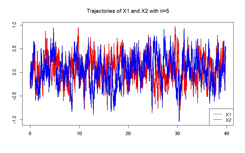
With this roadmap summary complete, the structure of this paper should appear as straightforward. We begin with a section of preliminaries presenting the tools needed from analysis on Wiener space, followed by a section covering the convergence in the continuous case, and then a section dealing with the case of discrete data. The final section provides some numerics to illustrate the convergence rates in practice, wherein we find that in discrete time, the time-scaled ρ~​(n)\tilde{\rho}\left(n\right) does indeed behave in distribution largely like a normal with variance θ−1\theta^{-1}, even without using the optimal observation frequency.

2 Preliminaries

2.1 Elements of Analysis on Wiener space

With (Ω,ℱ,𝐏)\left(\Omega,\mathcal{F},\mathbf{P}\right) denoting the Wiener space of a standard Wiener process WW, for a deterministic function h∈L2​(𝐑+)=:ℋh\in L^{2}\left(\mathbf{R}_{+}\right)=:{{\mathcal{H}}}, the Wiener integral ∫𝐑+h⁡(s)​𝑑W​(s)\int_{\mathbf{R}_{+}}h\left(s\right)dW\left(s\right) is also denoted by W⁡(h)W\left(h\right). The inner product ∫𝐑+f⁡(s)​g​(s)​𝑑s\int_{\mathbf{R}_{+}}f\left(s\right)g\left(s\right)ds will be denoted by ⟨f,g⟩ℋ\left\langle f,g\right\rangle_{{\mathcal{H}}}.

  • •

    The Wiener chaos expansion. For every q⩾1q\geqslant 1, ℋq{\mathcal{H}}_{q} denotes the qqth Wiener chaos of WW, defined as the closed linear subspace of L2​(Ω)L^{2}(\Omega) generated by the random variables {Hq​(W⁡(h)),h∈ℋ,‖h‖ℋ=1}\{H_{q}(W(h)),h\in{{\mathcal{H}}},\|h\|_{{\mathcal{H}}}=1\} where HqH_{q} is the qqth Hermite polynomial. Wiener chaos of different orders are orthogonal in L2​(Ω)L^{2}\left(\Omega\right). The so-called Wiener chaos expansion is the fact that any X∈L2​(Ω)X\in L^{2}\left(\Omega\right) can be written as

    X=𝐄⁡[X]+∑q=1∞XqX=\mathbf{E}[X]+\sum_{q=1}^{\infty}X_{q} (4)

    for some Xq∈ℋqX_{q}\in{\mathcal{H}}_{q} for every q⩾1q\geqslant 1. This is summarized in the direct-orthogonal-sum notation L2(Ω)=⊕q=0∞ℋqL^{2}\left(\Omega\right)=\oplus_{q=0}^{\infty}{\mathcal{H}}_{q}. Here ℋ0{\mathcal{H}}_{0} denotes the constants.

  • •

    Relation with Hermite polynomials. Multiple Wiener integrals. The mapping Iq​(h⊗q):=q!​Hq​(W⁡(h)){I_{q}(h^{\otimes q}):}=q!H_{q}(W(h)) is a linear isometry between the symmetric tensor product ℋ⊙q{\mathcal{H}}^{\odot q} (equipped with the modified norm ∥.∥ℋ⊙q=q!∥.∥ℋ⊗q\|.\|_{{\mathcal{H}}^{\odot q}}=\sqrt{q!}\|.\|_{{\mathcal{H}}^{\otimes q}}) and ℋq{\mathcal{H}}_{q}. Hence, for XX and its Wiener chaos expansion (4) above, each term XqX_{q} can be interpreted as a multiple Wiener integral Iq​(fq)I_{q}\left(f_{q}\right) for some fq∈ℋ⊙qf_{q}\in{\mathcal{H}}^{\odot q}.

  • •

    Isometry Property-Product formula. For any integers 1⩽q⩽p1\leqslant q\leqslant p and f∈ℋ⊙pf\in\mathcal{H}^{\odot p} and g∈ℋ⊙qg\in\mathcal{H}^{\odot q}, we have

    𝐄⁡[Ip​(f)​Iq​(g)]=\displaystyle\mathbf{E}[I_{p}(f)I_{q}(g)]= {p!​⟨f,g⟩ℋ⊗p if ​p=q0 otherwise.\displaystyle\left\{\begin{array}[]{ll}p!\langle f,g\rangle_{{\mathcal{H}^{\otimes p}}}&\mbox{ if }p=q\\ &\\ 0&\mbox{ }\text{otherwise}.\end{array}\right.

    For any integers pp, q⩾1q\geqslant 1 and symmetric integrands f∈ℋ⊙pf\in\mathcal{H}^{\odot p} and g∈ℋ⊙qg\in\mathcal{H}^{\odot q},

    Ip​(f)​Iq​(g)=∑r=0p∧qr!​Cpr​Cqr​Ip+q−2​r​(f​⊗r~​g);I_{p}(f)I_{q}(g)=\sum_{r=0}^{p\wedge q}r!{C}_{p}^{r}{C}_{q}^{r}I_{p+q-2r}(f\tilde{\otimes_{r}}g); (9)

    where f⊗rgf\otimes_{r}g is the contraction of order rr of ff and gg which is an element of ℋ⊗(p+q−2​r){\mathcal{H}}^{\otimes(p+q-2r)} defined by

    (f⊗rg)​(s1,…,sp−r,t1,…,tq−r)\displaystyle(f\otimes_{r}g)(s_{1},\ldots,s_{p-r},t_{1},\ldots,t_{q-r})
    =∫𝐑+p+q−2​rf(s1,…,sp−r,u1,…,ur)g(t1,…,tq−r,u1,…,ur)du1⋯dur.\displaystyle=\int_{\mathbf{R}_{+}^{p+q-2r}}f(s_{1},\ldots,s_{p-r},u_{1},\ldots,u_{r})g(t_{1},\ldots,t_{q-r},u_{1},\ldots,u_{r})\,du_{1}\cdots du_{r}.

    while (f​⊗r~​g)(f\tilde{\otimes_{r}}g) denotes its symmetrization. More generally the symmetrization f~\tilde{f} of a function ff is defined by f~​(x1,…,xp)=1p!​∑σf⁡(xσ⁡(1),…,xσ⁡(p))\tilde{f}(x_{1},...,x_{p})=\frac{1}{p!}\sum\limits_{\sigma}f(x_{\sigma(1)},...,x_{\sigma(p)}) where the sum runs over all permutations σ\sigma of {1,…,p}\{1,...,p\}. The special case for p=q=1p=q=1 in (9) is particularly handy, and can be written in its symmetrized form:

    I1​(f)​I1​(g)=2−1​I2​(f⊗g+g⊗f)+⟨f,g⟩ℋ.I_{1}(f)I_{1}(g)=2^{-1}I_{2}\left(f\otimes g+g\otimes f\right)+\langle f,g\rangle_{{\mathcal{H}}}. (10)

    where f⊗gf\otimes g means the tensor product of ff and gg.

  • •

    Hypercontractivity in Wiener chaos. For h∈ℋ⊗qh\in{\mathcal{H}}^{\otimes q}, the multiple Wiener integrals Iq​(h)I_{q}(h), which exhaust the set ℋq{\mathcal{H}}_{q}, satisfy a hypercontractivity property (equivalence in ℋq{\mathcal{H}}_{q} of all LpL^{p} norms for all p⩾2p\geqslant 2), which implies that for any F∈⊕l=1qℋlF\in\oplus_{l=1}^{q}{\mathcal{H}}_{l} (i.e. in a fixed sum of Wiener chaoses), we have

    (𝐄⁡[|F|p])1/p⩽cp,q​(𝐄⁡[|F|2])1/2​ for any ​p⩾2.\left(\mathbf{E}\big[|F|^{p}\big]\right)^{1/p}\leqslant c_{p,q}\left(\mathbf{E}\big[|F|^{2}\big]\right)^{1/2}\ \mbox{ for any }p\geqslant 2. (11)

    The constants cp,qc_{p,q} above are known with some precision when F∈ℋqF\in{\mathcal{H}}_{q}: by Corollary 2.8.14 in [8], cp,q=(p−1)q/2c_{p,q}=\left(p-1\right)^{q/2}.

  • •

    Malliavin derivative. For any function Φ∈C1​(𝐑)\Phi\in C^{1}\left(\mathbf{R}\right) with bounded derivative, and any h∈ℋh\in{\mathcal{H}}, the Malliavin derivative DD of the random variable X:=Φ⁡(W⁡(h))X:=\Phi\left(W\left(h\right)\right) is defined to be consistent with the following chain rule:

    D​X:X↦Dr​X:=Φ′​(W⁡(h))​h​(r)∈L2​(Ω×𝐑+).DX:X\mapsto D_{r}X:=\Phi^{\prime}\left(W\left(h\right)\right)h\left(r\right)\in L^{2}\left(\Omega\times\mathbf{R}_{+}\right).

    A similar chain rule holds for multivariate Φ\Phi. One then extends DD to the so-called Gross-Sobolev subset 𝐃1,2⫋L2​(Ω)\mathbf{D}^{1,2}\varsubsetneqq L^{2}\left(\Omega\right) by closing DD inside L2​(Ω)L^{2}\left(\Omega\right) under the norm defined by ‖X‖1,22:=𝐄⁡[X2]+∫𝐑+𝐄​|Dr​X|2​𝑑r.\left\|X\right\|_{1,2}^{2}:=\mathbf{E}\left[X^{2}\right]+\int_{\mathbf{R}_{+}}\mathbf{E|}D_{r}X|^{2}dr. All Wiener chaos random variable are in the domain 𝐃1,2\mathbf{D}^{1,2} of DD . In fact this domain can be expressed explicitly for any XX as in (4): X∈𝐃1,2X\in\mathbf{D}^{1,2} if and only if ∑qq​q!​‖fq‖ℋ⊗q2<∞\sum_{q}qq!\|f_{q}\|_{{\mathcal{H}}^{\otimes q}}^{2}<\infty.

  • •

    Generator LL of the Ornstein-Uhlenbeck semigroup. The linear operator LL is defined as being diagonal under the Wiener chaos expansion of L2​(Ω)L^{2}\left(\Omega\right): ℋq{\mathcal{H}}_{q} is the eigenspace of LL with eigenvalue −q-q, i.e. for any X∈ℋqX\in{\mathcal{H}}_{q} , L​X=−q​XLX=-qX. We have K​e​rKer(OPENL)=L)= ℋ0{\mathcal{H}}_{0}, the constants. The operator −L−1-L^{-1} is the negative pseudo-inverse of LL, so that for any X∈ℋqX\in{\mathcal{H}}_{q}, −L−1​X=q−1​X-L^{-1}X=q^{-1}X.

  • •

    Kolmogorov distance. Recall that, if X,YX,Y are two real-valued random variables, then the Kolmogorov distance between the law of XX and the law of YY is given by

    dK​o​l(X,Y)=supz∈𝐑|𝐏[X⩽z]−𝐏[Y⩽z]|d_{Kol}\left(X,Y\right)=\sup_{z\in\mathbf{R}}\left|\mathbf{P}\left[X\leqslant z\right]-\mathbf{P}\left[Y\leqslant z\right]\right|

    If X∈𝔻1,2X\in\mathbb{D}^{1,2}, with 𝐄⁡[X]=0\mathbf{E}[X]=0 and Y=𝒩⁡(0,1)Y=\mathcal{N}(0,1), then (Theorem 2.4 in [6]), then

    dK​o​l​(X,Y)⩽𝐄⁡[(1−⟨D​X,−D​L−1​X⟩ℋ)2]d_{Kol}\left(X,Y\right)\leqslant\sqrt{\mathbf{E}[(1-\langle DX,-DL^{-1}X\rangle_{\mathcal{H}})^{2}]}

    If moreover, X=Iq​(f)X=I_{q}(f) for some q⩾2q\geqslant 2, f∈ℋ⊙qf\in\mathcal{H}^{\odot q}, then ⟨D​X,−D​L−1​X⟩ℋ=q−1​‖D​X‖ℋ2\langle DX,-DL^{-1}X\rangle_{\mathcal{H}}=q^{-1}\|DX\|_{\mathcal{H}}^{2}, and thus in this case

    dK​o​l​(X,Y)⩽𝐄⁡[(1−q−1​‖D​X‖ℋ2)2]d_{Kol}\left(X,Y\right)\leqslant\sqrt{\mathbf{E}[(1-q^{-1}\|DX\|_{\mathcal{H}}^{2})^{2}]} (12)
Lemma 1

Let γ>0\gamma>0. Let (Zn)n∈ℕ(Z_{n})_{n\in\mathbb{N}} be a sequence of random variables. If for every p⩾1p\geqslant 1 there exists a constant cp>0c_{p}>0 such that for all n∈ℕn\in\mathbb{N},

‖Zn‖Lp​(Ω)⩽cp⋅n−γ,\|Z_{n}\|_{L^{p}(\Omega)}\leqslant c_{p}\cdot n^{-\gamma},

then for all ε>0\varepsilon>0 there exists a random variable ηε\eta_{\varepsilon} which is almost surely finite such that

|Zn|⩽ηε⋅n−γ+εalmost surely|Z_{n}|\leqslant\eta_{\varepsilon}\cdot n^{-\gamma+\varepsilon}\quad\mbox{almost surely}

for all n∈ℕn\in\mathbb{N}. Moreover, E​|ηε|p<∞E|\eta_{\varepsilon}|^{p}<\infty for all p⩾1p\geqslant 1.

3 Continuous observations

In this section, we compute the asymptotic variance of ρ⁡(T)\rho(T) and its normal fluctuations for large T,T, by working with each of the three terms which appear in its definition. For the sake of convienence and compactness of notation, we construct a two-sided Brownian motion (W⁡(t))t∈ℝ(W(t))_{t\in\mathbb{R}} from the two independent Brownian motions (W1​(t))t⩾0(W^{1}(t))_{t\geqslant 0} and (W2​(t))t⩾0(W^{2}(t))_{t\geqslant 0} as follows :

W(t):=W1(t)𝟏{t⩾0}+W2(−t)𝟏{t<0}, t∈ℝ.W(t):=W^{1}(t)\mathbf{1}_{\{t\geqslant 0\}}+W^{2}(-t)\mathbf{1}_{\{t<0\}},\text{ \ }t\in\mathbb{R.}

The following lemma will be convenient in the sequel.

Lemma 2

Let ff, gg ∈L2​(ℝ+)\in L^{2}(\mathbb{R}_{+}), then

I1W1​(f)​I1W2​(g)=I2W​(f¯⊗g¯¯)I_{1}^{W^{1}}(f)I_{1}^{W^{2}}(g)=I_{2}^{W}(\bar{f}\otimes\bar{\bar{g}})

where f¯\bar{f}, g¯¯\bar{\bar{g}} in L2​(ℝ)L^{2}(\mathbb{R}) are defined by

f¯(x)=f(x)𝟏{x⩾0}, g¯¯(x)=−g(−x)𝟏{x<0}.\bar{f}(x)=f(x)\mathbf{1}_{\{x\geqslant 0\}},\text{ \ }\bar{\bar{g}}(x)=-g(-x)\mathbf{1}_{\{x<0\}}.
Proof.

Using the product formula of multiple integrals, we have

I2W​(f¯⊗g¯¯)\displaystyle I_{2}^{W}(\bar{f}\otimes\bar{\bar{g}}) =\displaystyle= I1W​(f¯)​I1W​(g¯¯)−E⁡[I1W​(f¯)​I1W​(g¯¯)]\displaystyle I_{1}^{W}(\bar{f})I_{1}^{W}(\bar{\bar{g}})-E\left[I_{1}^{W}(\bar{f})I_{1}^{W}(\bar{\bar{g}})\right]
=\displaystyle= (∫ℝf¯​(x)​d​Wx)​(∫ℝg¯¯​(x)​d​Wx)−E​⟨f¯,g¯¯⟩L2​(ℝ)\displaystyle\left(\int_{\mathbb{R}}\bar{f}(x)dW_{x}\right)\left(\int_{\mathbb{R}}\bar{\bar{g}}(x)dW_{x}\right)-E\left<\bar{f},\bar{\bar{g}}\right>_{L^{2}(\mathbb{R})}
=\displaystyle= (∫0∞f⁡(x)​d​Wx1)​(∫0∞g⁡(x)​d​Wx2)\displaystyle\left(\int_{0}^{\infty}f(x)dW^{1}_{x}\right)\left(\int_{0}^{\infty}g(x)dW^{2}_{x}\right)
=\displaystyle= I1W1​(f)​I1W2​(g),\displaystyle I_{1}^{W^{1}}(f)I_{1}^{W^{2}}(g),

which completes the proof. ∎

3.1 Asymptotic distribution of Y12​(T)T\frac{Y_{12}(T)}{\sqrt{T}} :

The numerator of ρ⁡(T)\rho(T) can be written as follows

Y12​(T)T=FT−T​X1¯​(T)​X2¯​(T)\frac{Y_{12}(T)}{\sqrt{T}}=F_{T}-\sqrt{T}\bar{X_{1}}(T)\bar{X_{2}}(T) (13)

where FT:=1T​∫0TX1​(t)​X2​(t)​𝑑tF_{T}:=\frac{1}{\sqrt{T}}\int_{0}^{T}X_{1}(t)X_{2}(t)dt. Using the notation I1WI_{1}^{W} for the Wiener integral with respect to WW, since Xi​(t)=∫0te−θ⁡(t−u)​d​Wi​(u)X_{i}(t)=\int_{0}^{t}e^{-\theta(t-u)}dW^{i}(u) = I1Wi​(ft)I_{1}^{W^{i}}(f_{t}), i=1,2i=1,2 where ft(.):=e−θ(t−.)𝟏[0,t](.)f_{t}(.):=e^{-\theta(t-.)}\mathbf{1}_{[0,t]}(.) we can write using Lemma 2

FT\displaystyle F_{T} =1T​∫0TI1W1​(ft)​I1W2​(ft)​𝑑t\displaystyle=\frac{1}{\sqrt{T}}\int_{0}^{T}I_{1}^{W^{1}}(f_{t})I_{1}^{W^{2}}(f_{t})dt (14)
=I2W​(hT),\displaystyle=I_{2}^{W}(h_{T}),

with hT∈L2​([−T,T]2)h_{T}\in L^{2}([-T,T]^{2}) is given

hT:[−T,T]2\displaystyle h_{T}:[-T,T]^{2} →ℝ\displaystyle\rightarrow\mathbb{R}
(x,y)\displaystyle(x,y) ↦1T​∫0Tf¯t​(x)​f¯¯t​(y)​𝑑t\displaystyle\mapsto\frac{1}{\sqrt{T}}\int_{0}^{T}\bar{f}_{t}(x)\bar{\bar{f}}_{t}(y)dt (15)

On the other hand, we have

hT​(x,y)\displaystyle h_{T}(x,y) =1T∫0T−e−2​θ​teθ​xe−θ​y𝟏[0,t](x)𝟏[−t,0](y)dt\displaystyle=\frac{1}{\sqrt{T}}\int_{0}^{T}-e^{-2\theta t}e^{\theta x}e^{-\theta y}\mathbf{1}_{[0,t]}(x)\mathbf{1}_{[-t,0]}(y)dt
=1T∫0T−e−2​θ​teθ​xe−θ​y𝟏[x∨−y,T](t)𝟏[0,T](x)𝟏[−T,0](y)dt\displaystyle=\frac{1}{\sqrt{T}}\int_{0}^{T}-e^{-2\theta t}e^{\theta x}e^{-\theta y}\mathbf{1}_{[x\vee-y,T]}(t)\mathbf{1}_{[0,T]}(x)\mathbf{1}_{[-T,0]}(y)dt
=12​θ​1T​eθ​x​e−θ​y​[e−2​θ​T−e−2​θ​(x∨−y)]​𝟏[0,T]​(x)​𝟏[−T,0]​(y).\displaystyle=\frac{1}{2\theta}\frac{1}{\sqrt{T}}e^{\theta x}e^{-\theta y}\left[e^{-2\theta T}-e^{-2\theta(x\vee-y)}\right]\mathbf{1}_{[0,T]}(x)\mathbf{1}_{[-T,0]}(y).

Note that the kernel hTh_{T} is not symmetric, in the sequel we will denote h~T\tilde{h}_{T} its systematization defined by h~T​(x,y):=12​(hT​(x,y)+hT​(y,x))\tilde{h}_{T}(x,y):=\frac{1}{2}(h_{T}(x,y)+h_{T}(y,x)). We are now ready to compute the asymptotic variance of the main term in the numerator of ρ\rho.

Lemma 3

With FTF_{T} defined in (14), then

|𝐄⁡[FT2]−14​θ3|⩽C⁡(θ)T,\left|\mathbf{E}[F_{T}^{2}]-\frac{1}{4\theta^{3}}\right|\leqslant\frac{C(\theta)}{T},

where C⁡(θ):=7+8​θ16​θ4C(\theta):=\frac{7+8\theta}{16\theta^{4}}. In particular, limT→∞𝐄⁡[FT2]=14​θ3\lim_{T\rightarrow\infty}\mathbf{E}[F_{T}^{2}]=\frac{1}{4\theta^{3}}.

Proof.

We have

𝐄⁡[FT2]\displaystyle\mathbf{E}[F_{T}^{2}] =𝐄⁡[I2W​(hT)2]\displaystyle=\mathbf{E}[I_{2}^{W}(h_{T})^{2}]
=2×‖h~T‖L2​([−T,T]2)2\displaystyle=2\times\|\tilde{h}_{T}\|_{L^{2}([-T,T]^{2})}^{2}
=1T​14​θ2​∫−T0∫0Te2​θ​x​e−2​θ​y​[e−2​θ​T−e−2​θ​(x∨−y)]2​𝑑x​𝑑y\displaystyle=\frac{1}{T}\frac{1}{4\theta^{2}}\int_{-T}^{0}\int_{0}^{T}e^{2\theta x}e^{-2\theta y}\left[e^{-2\theta T}-e^{-2\theta(x\vee-y)}\right]^{2}dxdy
=1T​14​θ2​∫0T∫0Te2​θ​x​e2​θ​z​[e−2​θ​T−e−2​θ​(x∨z)]2​𝑑x​𝑑z\displaystyle=\frac{1}{T}\frac{1}{4\theta^{2}}\int_{0}^{T}\int_{0}^{T}e^{2\theta x}e^{2\theta z}\left[e^{-2\theta T}-e^{-2\theta(x\vee z)}\right]^{2}dxdz
=1T​12​θ2​∫0T∫0ze2​θ​x​e2​θ​z​[e−2​θ​T−e−2​θ​z]2​𝑑x​𝑑z\displaystyle=\frac{1}{T}\frac{1}{2\theta^{2}}\int_{0}^{T}\int_{0}^{z}e^{2\theta x}e^{2\theta z}\left[e^{-2\theta T}-e^{-2\theta z}\right]^{2}dxdz
=1T​14​θ3​[∫0T(e−2​θ​(T−y)−1)2​𝑑y−∫0Te−2​θ​y​(e−2​θ​(T−y)−1)2​𝑑y]\displaystyle=\frac{1}{T}\frac{1}{4\theta^{3}}\left[\int_{0}^{T}(e^{-2\theta(T-y)}-1)^{2}dy-\int_{0}^{T}e^{-2\theta y}(e^{-2\theta(T-y)}-1)^{2}dy\right]
=:A1​(T)+A2​(T)\displaystyle=:A_{1}(T)+A_{2}\left(T\right)

where

|A1​(T)−14​θ3|\displaystyle|A_{1}(T)-\frac{1}{4\theta^{3}}| :=|1T​14​θ3​∫0T(e−2​θ​(T−y)−1)2​𝑑y−14​θ3|\displaystyle:=\left|\frac{1}{T}\frac{1}{4\theta^{3}}\int_{0}^{T}(e^{-2\theta(T-y)}-1)^{2}dy-\frac{1}{4\theta^{3}}\right|
=|1T​14​θ3​[14​θ​(1−e−4​θ​T)+1θ​(e−2​θ​T−1)+T]−14​θ3|\displaystyle=\left|\frac{1}{T}\frac{1}{4\theta^{3}}[\frac{1}{4\theta}(1-e^{-4\theta T})+\frac{1}{\theta}(e^{-2\theta T}-1)+T]-\frac{1}{4\theta^{3}}\right|
⩽516​θ4×1T,\displaystyle\leqslant\frac{5}{16\theta^{4}}\times\frac{1}{T},

and

|A2​(T)|\displaystyle|A_{2}(T)| :=|1T​14​θ3​∫0Te−2​θ​y​(e−2​θ​(T−y)−1)2​𝑑y|\displaystyle:=\left|\frac{1}{T}\frac{1}{4\theta^{3}}\int_{0}^{T}e^{-2\theta y}(e^{-2\theta(T-y)}-1)^{2}dy\right|
⩽1T​18​θ4​(1−e−4​θ​T)+12​θ3​e−2​θ​T\displaystyle\leqslant\frac{1}{T}\frac{1}{8\theta^{4}}(1-e^{-4\theta T})+\frac{1}{2\theta^{3}}e^{-2\theta T}
⩽(1+4​θ)8​θ4×1T.\displaystyle\leqslant\frac{(1+4\theta)}{8\theta^{4}}\times\frac{1}{T}.

∎

Proposition 4

Let FTθ:=2​θ3/2​FTF^{\theta}_{T}:=2\theta^{3/2}F_{T} and N∼𝒩⁡(0,1)N\sim\mathcal{N}(0,1), then we have

dK​o​l​(FTθ,N)⩽c⁡(θ)T.d_{Kol}(F^{\theta}_{T},N)\leqslant\frac{c(\theta)}{\sqrt{T}}.

where c⁡(θ):=(2+74​θ)2+334​θc(\theta):=\sqrt{(2+\frac{7}{4\theta})^{2}+\frac{3^{3}}{4\theta}}. Consequently FT​⟶ℒ​𝒩​(0,14​θ3)F_{T}\overset{\mathcal{L}}{\longrightarrow}\mathcal{N}\left(0,\frac{1}{4\theta^{3}}\right) as T→+∞T\rightarrow+\infty.

Proof.

We will use the estimate (12) recalled in the preliminaries in order to prove this proposition. We have DtFTθ=4θ3/2I1W(h~T(.,t))D_{t}F_{T}^{\theta}=4\theta^{3/2}I_{1}^{W}(\tilde{h}_{T}(.,t)), t∈[−T,T]t\in[-T,T], hence

12​‖D​FTθ‖L2​([−T,T])2\displaystyle\frac{1}{2}\|DF_{T}^{\theta}\|_{L^{2}([-T,T])}^{2} =12​∫−TT(Dt​FTθ)2​𝑑t\displaystyle=\frac{1}{2}\int_{-T}^{T}(D_{t}F_{T}^{\theta})^{2}dt
=8θ3∫−TTI1W(h~T(.,t))2dt\displaystyle=8\theta^{3}\int_{-T}^{T}I_{1}^{W}(\tilde{h}_{T}(.,t))^{2}dt
=8θ3[∫−TTI2W(h~T(.,t)⊗h~T(.,t))dt+∫−TT∥h~T(.,t)∥L2​([−T,T])2]\displaystyle=8\theta^{3}\left[\int_{-T}^{T}I_{2}^{W}(\tilde{h}_{T}(.,t)\otimes\tilde{h}_{T}(.,t))dt+\int_{-T}^{T}\|\tilde{h}_{T}(.,t)\|_{L^{2}([-T,T])}^{2}\right]
=8​θ3​[I2W​(h~T⊗1h~T)+‖h~T‖L2​([−T,T]2)2],\displaystyle=8\theta^{3}\left[I_{2}^{W}(\tilde{h}_{T}\otimes_{1}\tilde{h}_{T})+\|\tilde{h}_{T}\|_{L^{2}([-T,T]^{2})}^{2}\right],

where we used the product formula (10) and the fact that the kernel h~T⊗1h~T\tilde{h}_{T}\otimes_{1}\tilde{h}_{T} is symmetric. Thus

𝐄⁡[(1−12​‖D​FTθ‖L2​([−T,T])2)2]=(𝐄⁡[(FTθ)2]−1)2+27​θ6×‖h~T⊗1h~T‖L2​([−T,T]2)2\mathbf{E}\left[(1-\frac{1}{2}\|DF_{T}^{\theta}\|_{L^{2}([-T,T])}^{2})^{2}\right]=(\mathbf{E}[(F_{T}^{\theta})^{2}]-1)^{2}+2^{7}\theta^{6}\times\|\tilde{h}_{T}\otimes_{1}\tilde{h}_{T}\|_{L^{2}([-T,T]^{2})}^{2} (16)

We have,

(h~T⊗1h~T)​(x,y)\displaystyle(\tilde{h}_{T}\otimes_{1}\tilde{h}_{T})(x,y)
=∫[−T,T]h~T​(x,z)​h~T​(y,z)​𝑑z\displaystyle=\int_{[-T,T]}\tilde{h}_{T}(x,z)\tilde{h}_{T}(y,z)dz
=14​∫[−T,0]hT​(x,z)​hT​(y,z)​𝟏[0,T]​(x)​𝟏[0,T]​(y)​𝑑z+14​∫[0,T]hT​(z,x)​hT​(z,y)​𝟏[−T,0]​(x)​𝟏[−T,0]​(y)​𝑑z\displaystyle=\frac{1}{4}\int_{[-T,0]}h_{T}(x,z)h_{T}(y,z)\mathbf{1}_{[0,T]}(x)\mathbf{1}_{[0,T]}(y)dz+\frac{1}{4}\int_{[0,T]}h_{T}(z,x)h_{T}(z,y)\mathbf{1}_{[-T,0]}(x)\mathbf{1}_{[-T,0]}(y)dz

Hence

‖h~T⊗1h~T‖L2​([−T,T]2)2\displaystyle\|\tilde{h}_{T}\otimes_{1}\tilde{h}_{T}\|_{L^{2}([-T,T]^{2})}^{2} (17)
⩽18​∫[0,T]2(∫[−T,0]hT​(x,z)​hT​(y,z))2​𝑑x​𝑑y+18​∫[−T,0]2(∫[0,T]hT​(z,x)​hT​(z,y))2​𝑑x​𝑑y\displaystyle\leqslant\frac{1}{8}\int_{[0,T]^{2}}\left(\int_{[-T,0]}h_{T}(x,z)h_{T}(y,z)\right)^{2}dxdy+\frac{1}{8}\int_{[-T,0]^{2}}\left(\int_{[0,T]}h_{T}(z,x)h_{T}(z,y)\right)^{2}dxdy

On the other hand by Fubini’s theorem

∫[0,T]2(∫[−T,0]hT​(x,z)​hT​(y,z)​𝑑z)2​𝑑x​𝑑y=1T2​∫[0,T]2[∫[−T,0]∫[0,T]2f¯r​(x)​f¯¯r​(z)​f¯s​(y)​f¯¯s​(z)​𝑑r​𝑑s​𝑑z]2​𝑑x​𝑑y\displaystyle\int_{[0,T]^{2}}\left(\int_{[-T,0]}h_{T}(x,z)h_{T}(y,z)dz\right)^{2}dxdy=\frac{1}{T^{2}}\int_{[0,T]^{2}}\left[\int_{[-T,0]}\int_{[0,T]^{2}}\bar{f}_{r}(x)\bar{\bar{f}}_{r}(z)\bar{f}_{s}(y)\bar{\bar{f}}_{s}(z)drdsdz\right]^{2}dxdy
=1T2​∫[0,T]2(∫[0,T]2f¯r​(x)​f¯s​(y)​⟨f¯¯r,f¯¯s⟩L2​([−T,0])​𝑑r​𝑑s)2​𝑑x​𝑑y\displaystyle=\frac{1}{T^{2}}\int_{[0,T]^{2}}\left(\int_{[0,T]^{2}}\bar{f}_{r}(x)\bar{f}_{s}(y)\langle\bar{\bar{f}}_{r},\bar{\bar{f}}_{s}\rangle_{L^{2}([-T,0])}drds\right)^{2}dxdy
=1T2​∫[0,T]2∫[0,T]4f¯r​(x)​f¯s​(y)​f¯v​(x)​f¯u​(y)​⟨f¯¯r,f¯¯s⟩L2​([−T,0])​⟨f¯¯v,f¯¯u⟩L2​([−T,0])​𝑑r​𝑑s​𝑑u​𝑑v​𝑑x​𝑑y\displaystyle=\frac{1}{T^{2}}\int_{[0,T]^{2}}\int_{[0,T]^{4}}\bar{f}_{r}(x)\bar{f}_{s}(y)\bar{f}_{v}(x)\bar{f}_{u}(y)\langle\bar{\bar{f}}_{r},\bar{\bar{f}}_{s}\rangle_{L^{2}([-T,0])}\langle\bar{\bar{f}}_{v},\bar{\bar{f}}_{u}\rangle_{L^{2}([-T,0])}drdsdudvdxdy

Using the fact that the other term of (17) can be treated similarly and that ⟨f¯¯r,f¯¯s⟩L2​([−T,0])=⟨f¯r,f¯s⟩L2​([0,T])=𝐄⁡[Xi​(r)​Xi​(s)]\langle\bar{\bar{f}}_{r},\bar{\bar{f}}_{s}\rangle_{L^{2}([-T,0])}=\langle{\bar{f}}_{r},{\bar{f}}_{s}\rangle_{L^{2}([0,T])}=\mathbf{E}[X^{i}(r)X^{i}(s)], i=1,2i=1,2, we get

‖h~T⊗1h~T‖L2​([−T,T]2)2\displaystyle\|\tilde{h}_{T}\otimes_{1}\tilde{h}_{T}\|_{L^{2}([-T,T]^{2})}^{2}
⩽14​1T2​∫[0,T]4𝐄⁡[Xi​(r)​Xi​(v)]​𝐄​[Xi​(s)​Xi​(u)]​𝐄​[Xi​(r)​Xi​(s)]​𝐄​[Xi​(v)​Xi​(u)]​𝑑r​𝑑s​𝑑u​𝑑v\displaystyle\leqslant\frac{1}{4}\frac{1}{T^{2}}\int_{[0,T]^{4}}\mathbf{E}[X^{i}(r)X^{i}(v)]\mathbf{E}[X^{i}(s)X^{i}(u)]\mathbf{E}[X^{i}(r)X^{i}(s)]\mathbf{E}[X^{i}(v)X^{i}(u)]drdsdudv

On the other hand, since for i=1,2i=1,2, 𝐄⁡[Xi​(r)​Xi​(s)]=e−θ⁡(r+s)2​θ​[e2​θ​(r∧s)−1]⩽12​θ​e−θ​|r−s|=𝐄⁡[Zi​(r)​Zi​(s)]:=Q⁡(r−s)\mathbf{E}[X^{i}(r)X^{i}(s)]=\frac{e^{-\theta(r+s)}}{2\theta}[e^{2\theta(r\wedge s)}-1]\leqslant\frac{1}{2\theta}e^{-\theta|r-s|}=\mathbf{E}[Z_{i}(r)Z_{i}(s)]:=Q(r-s), where Zi​(r):=∫−∞re−θ⁡(r−t)​d​Wi​(t)Z_{i}(r):=\int_{-\infty}^{r}e^{-\theta(r-t)}dW^{i}(t), i=1,2i=1,2 we get

‖h~T⊗1h~T‖L2​([−T,T]2)2\displaystyle\|\tilde{h}_{T}\otimes_{1}\tilde{h}_{T}\|_{L^{2}([-T,T]^{2})}^{2} (18)
⩽14​1T2​∫[0,T]4Q⁡(u−v)​Q​(v−r)​Q​(r−s)​Q​(s−u)​𝑑u​𝑑v​𝑑r​𝑑s\displaystyle\leqslant\frac{1}{4}\frac{1}{T^{2}}\int_{[0,T]^{4}}Q(u-v)Q(v-r)Q(r-s)Q(s-u)dudvdrds (19)
=14​1T2​∫[0,T]2d​u​𝑑r​∫ℝ2d​v​𝑑s​QT​(u−v)​QT​(s−r)​QT​(u−s)​QT​(v−r)\displaystyle=\frac{1}{4}\frac{1}{T^{2}}\int_{[0,T]^{2}}dudr\int_{\mathbb{R}^{2}}dvdsQ_{T}(u-v)Q_{T}(s-r)Q_{T}(u-s)Q_{T}(v-r) (20)
=14​1T2​∫[0,T]2d​u​𝑑r​∫ℝ2d​v​𝑑s​QT​(y)​QT​(u−r−x)​QT​(x)​QT​(u−r−y),\displaystyle=\frac{1}{4}\frac{1}{T^{2}}\int_{[0,T]^{2}}dudr\int_{\mathbb{R}^{2}}dvdsQ_{T}(y)Q_{T}(u-r-x)Q_{T}(x)Q_{T}(u-r-y), (21)

where QT(x):=|Q(x)|𝟏{|x|⩽T}Q_{T}(x):=|Q(x)|\mathbf{1}_{\{|x|\leqslant T\}} and we used the change of variables y=u−vy=u-v, x=u−sx=u-s. Therefore, applying Young’s inequality, we can conclude

‖h~T⊗1h~T‖L2​([−T,T]2)2\displaystyle\|\tilde{h}_{T}\otimes_{1}\tilde{h}_{T}\|_{L^{2}([-T,T]^{2})}^{2} ⩽\displaystyle\leqslant 14​1T2​∫[0,T]2d​u​𝑑r​(QT∗QT)​(u−r)2\displaystyle\frac{1}{4}\frac{1}{T^{2}}\int_{[0,T]^{2}}dudr(Q_{T}\ast Q_{T})(u-r)^{2} (22)
⩽\displaystyle\leqslant 14​1T​∫ℝ(QT∗QT)​(z)2​𝑑z\displaystyle\frac{1}{4}\frac{1}{T}\int_{\mathbb{R}}(Q_{T}\ast Q_{T})(z)^{2}dz
=\displaystyle= 14​1T​‖QT∗QT‖L2​(ℝ)2\displaystyle\frac{1}{4}\frac{1}{T}\|Q_{T}\ast Q_{T}\|_{L^{2}(\mathbb{R})}^{2}
⩽\displaystyle\leqslant 14​1T​‖QT‖L4/3​(ℝ)4=14​1T​(∫[−T,T]|Q⁡(t)|4/3​𝑑t)3/4\displaystyle\frac{1}{4}\frac{1}{T}\|Q_{T}\|_{L^{4/3}(\mathbb{R})}^{4}=\frac{1}{4}\frac{1}{T}\left(\int_{[-T,T]}|Q(t)|^{4/3}dt\right)^{3/4}
=\displaystyle= 141T(3327​θ7(1−e−4θT/3)3).\displaystyle\frac{1}{4}\frac{1}{T}\left(\frac{3^{3}}{2^{7}\theta^{7}}(1-e^{-4\theta T/3})^{3}\right).

The desired result follows using (12) and the estimates (16), (22) and Lemma 14. ∎

We will need the following Proposition due to Michel and Pfanzagl (1971) [11] in the sequel which gives upper bounds for Kolmogorov’s distance between respectively the sum and the ratio of two random variables and a standard Gaussian random variable.

Proposition 5

Let XX, YY and ZZ be three random variables defined on a probability space (Ω,ℱ,𝐏)(\Omega,\mathcal{F},\mathbf{P}) such that 𝐏⁡(Z>0)=1\mathbf{P}(Z>0)=1. Then, for all ε>0\varepsilon>0, we have

  1. 1.

    dK​o​l​(X+Y,N)⩽dK​o​l​(X,N)+𝐏⁡(|Y|>ε)+εd_{Kol}(X+Y,N)\leqslant d_{Kol}(X,N)+\mathbf{P}(|Y|>\varepsilon)+\varepsilon.

  2. 2.

    dK​o​l​(XZ,N)⩽dK​o​l​(X,N)+𝐏⁡(|Z−1|>ε)+ε.d_{Kol}(\frac{X}{Z},N)\leqslant d_{Kol}(X,N)+\mathbf{P}(|Z-1|>\varepsilon)+\varepsilon.

where N∼𝒩⁡(0,1).N\sim\mathcal{N}(0,1).

Proposition 6

Let YY be a r.v. such that Y=N×N′Y=N\times N^{\prime} where N∼𝒩⁡(0,σ12)N\sim\mathcal{N}(0,\sigma^{2}_{1}) and N′∼𝒩⁡(0,σ22)N^{\prime}\sim\mathcal{N}(0,\sigma^{2}_{2}) two independent Gaussian r.v defined on a probability space (Ω,ℱ,𝐏)(\Omega,\mathcal{F},\mathbf{P}). Then, there exists a constant β>2​33​σ1​σ2\beta>\frac{2\sqrt{3}}{3}\sigma_{1}\sigma_{2} such that

𝐄⁡[eYβ]<2.\mathbf{E}\left[e^{\frac{Y}{\beta}}\right]<2.

Moreover, there exists a constant C>33​πC>\frac{\sqrt{3}}{3}\pi such that β<C×𝐄⁡[|Y|]\beta<C\times\mathbf{E}[|Y|].

Proof.

By the independence of NN and N′N^{\prime}, it’s easy to check that for any β>σ1​σ2\beta>\sigma_{1}\sigma_{2}, we have

𝐄⁡[eYβ]\displaystyle\mathbf{E}\left[e^{\frac{Y}{\beta}}\right] =12​π​σ1​σ2​∫ℝ2ex​yβ​e−x22​σ12​e−y22​σ22​𝑑x​𝑑y\displaystyle=\frac{1}{2\pi\sigma_{1}\sigma_{2}}\int_{\mathbb{R}^{2}}e^{\frac{xy}{\beta}}e^{-\frac{x^{2}}{2\sigma^{2}_{1}}}e^{-\frac{y^{2}}{2\sigma^{2}_{2}}}dxdy
=1(1−σ12​σ22β2).\displaystyle=\frac{1}{\sqrt{(1-\frac{\sigma^{2}_{1}\sigma^{2}_{2}}{\beta^{2}})}}.

Thus the constraint 𝐄⁡[eYβ]<2\mathbf{E}\left[e^{\frac{Y}{\beta}}\right]<2 implies that β\beta should be such that β>2​33​σ1​σ2\beta>\frac{2\sqrt{3}}{3}\sigma_{1}\sigma_{2}. On the other hand since 𝐄⁡[|Y|]=𝐄⁡[|N|]×𝐄⁡[|N′|]=2​σ1​σ2π\mathbf{E}[|Y|]=\mathbf{E}[|N|]\times\mathbf{E}[|N^{\prime}|]=\frac{2\sigma_{1}\sigma_{2}}{\pi}, thus there exists a constant C>33​πC>\frac{\sqrt{3}}{3}\pi such that β<C×𝐄⁡[|Y|]\beta<C\times\mathbf{E}[|Y|]. ∎

Corollary 7

Let XX,YY be two r.v. defined on a probability space (Ω,ℱ,𝐏)(\Omega,\mathcal{F},\mathbf{P}) such that Y=N×N′Y=N\times N^{\prime} where N∼𝒩⁡(0,σ12)N\sim\mathcal{N}(0,\sigma_{1}^{2}) and N′∼𝒩⁡(0,σ22)N^{\prime}\sim\mathcal{N}(0,\sigma_{2}^{2}). Then, there exists a constant 2​33​σ1​σ2<β⩽((C×𝐄⁡[|Y|])∧4)\frac{2\sqrt{3}}{3}\sigma_{1}\sigma_{2}<\beta\leqslant\left((C\times\mathbf{E}[|Y|])\wedge 4\right) such that

dK​o​l​(X+Y,𝒩⁡(0,1))⩽dK​o​l​(X,𝒩⁡(0,1))+β⁡(1+ln⁡(4β)).d_{Kol}(X+Y,\mathcal{N}(0,1))\leqslant d_{Kol}(X,\mathcal{N}(0,1))+\beta\left(1+\ln\left(\frac{4}{\beta}\right)\right).
Proof.

Let XX, YY be two random variables , then from Michel and Pfanzagl (1971), for all ε>0\varepsilon>0,

dK​o​l​(X+Y,𝒩⁡(0,1))⩽dK​o​l​(X,𝒩⁡(0,1))+𝐏⁡(|Y|>ε)+ε.d_{Kol}(X+Y,\mathcal{N}(0,1))\leqslant d_{Kol}(X,\mathcal{N}(0,1))+\mathbf{P}(|Y|>\varepsilon)+\varepsilon.

Since Y=N×N′Y=N\times N^{\prime} where N∼𝒩⁡(0,σ12)N\sim\mathcal{N}(0,\sigma^{2}_{1}) and N′∼𝒩⁡(0,σ22)N^{\prime}\sim\mathcal{N}(0,\sigma^{2}_{2}) then, by Proposition 6 and Markov’s inequality, we have

𝐏⁡(|Y|>ε)=2×𝐏⁡(Y>ε)⩽2×𝐄⁡[eYβ]​e−εβ<4​e−εβ.\mathbf{P}(|Y|>\varepsilon)=2\times\mathbf{P}(Y>\varepsilon)\leqslant 2\times\mathbf{E}\left[e^{\frac{Y}{\beta}}\right]e^{-\frac{\varepsilon}{\beta}}<4e^{-\frac{\varepsilon}{\beta}}.

Thus we can write

dK​o​l​(X+Y,𝒩⁡(0,1))⩽dK​o​l​(X,𝒩⁡(0,1))+infε>0gβ​(ε).d_{Kol}(X+Y,\mathcal{N}(0,1))\leqslant d_{Kol}(X,\mathcal{N}(0,1))+\inf_{\varepsilon>0}g_{\beta}(\varepsilon).

where gβ​(ε):=4​e−εβ+ε.g_{\beta}(\varepsilon):=4e^{-\frac{\varepsilon}{\beta}}+\varepsilon. Since gβg_{\beta} is convex on ℝ+\mathbb{R}_{+}, arginfε>0gβ(ε)=ε∗(β)=βln(4β)\arg\inf\limits_{\varepsilon>0}g_{\beta}(\varepsilon)=\varepsilon^{*}(\beta)=\beta\ln(\frac{4}{\beta}), β<((C×𝐄⁡[|Y|])∧4)\beta<\left((C\times\mathbf{E}[|Y|])\wedge 4\right), with CC the constant from Proposition 6. The desired result follows. ∎

To prove the convergence in law of Y12​(T)T\frac{Y_{12}(T)}{\sqrt{T}}, recall that T−1/2Y12(T)=FT−TX1¯(T)X2¯(T).T^{-1/2}Y_{12}(T)=F_{T}-\sqrt{T}\bar{X_{1}}(T)\bar{X_{2}}(T). We can write Xi¯​(T):=I1Wi​(gT)\bar{X_{i}}(T):=I_{1}^{W_{i}}(g_{T}), i=1,2i=1,2 where gT:=T−1​∫0Tft​𝑑tg_{T}:=T^{-1}\int_{0}^{T}f_{t}dt and we have for i=1,2i=1,2

𝐄​[Xi¯2​(T)]\displaystyle\mathbf{E}[\bar{X_{i}}^{2}(T)] =‖gT‖L2​([0,T])2\displaystyle=\|g_{T}\|_{L^{2}([0,T])}^{2}
=1T2​∫0T(∫0Tft​(u)​𝑑t)2​𝑑u\displaystyle=\frac{1}{T^{2}}\int_{0}^{T}(\int_{0}^{T}f_{t}(u)dt)^{2}du
=1T2​∫0Te2​θ​u​(∫uTe−θ​t​𝑑t)2​𝑑u\displaystyle=\frac{1}{T^{2}}\int_{0}^{T}e^{2\theta u}(\int_{u}^{T}e^{-\theta t}dt)^{2}du
=1T2​1θ2​∫0T(1−e−θ⁡(T−u))2​𝑑u⩽1θ2​1T.\displaystyle=\frac{1}{T^{2}}\frac{1}{\theta^{2}}\int_{0}^{T}(1-e^{-\theta(T-u)})^{2}du\leqslant\frac{1}{\theta^{2}}\frac{1}{T}. (23)

Hence by the independence of X1X_{1} and X2X_{2} and denoting Y⁡(T):=T​X1¯​(T)​X2¯​(T)Y(T):=\sqrt{T}\bar{X_{1}}(T)\bar{X_{2}}(T), we get

𝐄⁡[Y​(T)2]⩽1T​1θ4.\mathbf{E}[Y(T)^{2}]\leqslant\frac{1}{T}\frac{1}{\theta^{4}}. (24)

Then in virtue of Proposition 6 and Corollary 7, there exists a constant β\beta with 4​33​T​θ3/2​‖gT‖L2​([0,T])2<β<CT​θ2∧4\frac{4\sqrt{3}}{3}\sqrt{T}\theta^{3/2}\|g_{T}\|_{L^{2}([0,T])}^{2}<\beta<\frac{C}{\sqrt{T}\theta^{2}}\wedge 4 such that

dK​o​l​(Y12​(T)T,𝒩⁡(0,14​θ3))⩽dK​o​l​(FT,𝒩⁡(0,14​θ3))+β⁡(1+ln⁡(4β)).d_{Kol}\left(\frac{Y_{12}(T)}{\sqrt{T}},\mathcal{N}(0,\frac{1}{4\theta^{3}})\right)\leqslant d_{Kol}\left(F_{T},\mathcal{N}(0,\frac{1}{4\theta^{3}})\right)+\beta\left(1+\ln\left(\frac{4}{\beta}\right)\right).

On the other hand, since the function x↦x⁡(1+ln⁡(4x))x\mapsto x(1+\ln(\frac{4}{x})) is increasing on (0,4)(0,4), we have for TT large enough

dK​o​l​(Y12​(T)T,𝒩⁡(0,14​θ3))⩽dK​o​l​(FT,𝒩⁡(0,14​θ3))+c⁡(θ)2​ln⁡(T)T.d_{Kol}\left(\frac{Y_{12}(T)}{\sqrt{T}},\mathcal{N}(0,\frac{1}{4\theta^{3}})\right)\leqslant d_{Kol}\left(F_{T},\mathcal{N}(0,\frac{1}{4\theta^{3}})\right)+\frac{c(\theta)}{2}\frac{\ln(T)}{\sqrt{T}}.

The following proposition follows.

Proposition 8

There exists a constant C⁡(θ)C(\theta) depending only on θ\theta, such that

dK​o​l​(Y12​(T)T,𝒩⁡(0,14​θ3))⩽C⁡(θ)×ln⁡(T)T.d_{Kol}\left(\frac{Y_{12}(T)}{\sqrt{T}},\mathcal{N}\left(0,\frac{1}{4\theta^{3}}\right)\right)\leqslant C(\theta)\times\frac{\ln(T)}{\sqrt{T}}.

In particular, Y12​(T)T​⟶ℒ​𝒩​(0,14​θ3)\frac{Y_{12}(T)}{\sqrt{T}}\overset{\mathrm{\mathcal{L}}}{\longrightarrow}\mathcal{N}(0,\frac{1}{4\theta^{3}}) as T→+∞T\rightarrow+\infty.

Having just completed the study of the convergence in law of the numerator in ρ⁡(T)\rho(T), in order to study the convergence in law of T​ρ​(T)\sqrt{T}\rho(T), we will use Proposition 5 assertion 2 and the fact that

θ​T​ρ​(T)=2​θ3/2​Y12​(T)T2​θ​Y11​(T)T×Y22​(T)T\sqrt{\theta}\sqrt{T}\rho(T)=\frac{2\theta^{3/2}\frac{Y_{12}(T)}{\sqrt{T}}}{2\theta\sqrt{\frac{Y_{11}(T)}{T}\times\frac{Y_{22}(T)}{T}}} (25)

to show in the next subsection that the denominator concentrates to the value 1, and that the behavior of T​ρ​(T)\sqrt{T}\rho(T) is thus given by that of the numerator above.

3.2 The denominator term

Let us denote the denominator term

D⁡(T):=D:=2​θ​Y11​(T)×Y22​(T)T×T,D(T):=D:=2\theta\sqrt{\frac{Y_{11}(T)\times Y_{22}(T)}{T\times T}}, (26)

According to Proposition 5 assertion 2. we need to estimate 𝐏⁡(|D−1|>ε)\mathbf{P}(|D-1|>\varepsilon) for instance for 0<ε<10<\varepsilon<1. Using the fact that D⩾0D\geqslant 0 a.s. then |D−1|⩽|D2−1||D-1|\leqslant|D^{2}-1| a.s. Now using the shorthand notation Y¯i​i​(T):=Yi​i​(T)T/2​θ\bar{Y}_{ii}(T):=\frac{Y_{ii}(T)}{T/2\theta}, i=1,2i=1,2, thus, we have a.s.

|D−1|⩽|D2−1|\displaystyle|D-1|\leqslant|D^{2}-1| ⩽|Y¯11​(T)​Y¯22​(T)−1|\displaystyle\leqslant|\bar{Y}_{11}(T)\bar{Y}_{22}(T)-1|
⩽|Y¯11​(T)−1|×|Y¯22​(T)−1|+|Y¯11​(T)−1|+|Y¯22​(T)−1|\displaystyle\leqslant|\bar{Y}_{11}(T)-1|\times|\bar{Y}_{22}(T)-1|+|\bar{Y}_{11}(T)-1|+|\bar{Y}_{22}(T)-1| (27)

Thus, using the fact that Y¯11​(T)\bar{Y}_{11}(T) and Y¯22​(T)\bar{Y}_{22}(T) are equal in law, we get for any ε<1\varepsilon<1,

𝐏⁡(|D−1|>ε)\displaystyle\mathbf{P}\left(|D-1|>\varepsilon\right) ⩽𝐏⁡(|Y¯11​(T)−1|>ε3)+𝐏⁡(|Y¯22​(T)−1|>ε3)+2​𝐏​(|Y¯11​(T)−1|2>ε3)\displaystyle\leqslant\mathbf{P}\left(|\bar{Y}_{11}(T)-1|>\frac{\varepsilon}{3}\right)+\mathbf{P}\left(|\bar{Y}_{22}(T)-1|>\frac{\varepsilon}{3}\right)+2\mathbf{P}\left(|\bar{Y}_{11}(T)-1|^{2}>\frac{\varepsilon}{3}\right)
⩽4×𝐏⁡(|Y¯11​(T)−1|>ε3).\displaystyle\leqslant 4\times\mathbf{P}\left(|\bar{Y}_{11}(T)-1|>\frac{\varepsilon}{3}\right). (28)

We lighten the notation by writing ε\varepsilon instead of ε/3\varepsilon/3, therefore by Proposition 5 assertion 2. applied to ρ⁡(T)\rho(T) in (25), we get

dK​o​l​(θ​T​ρ​(T),N)⩽dK​o​l​(2​θ3/2​Y12​(T)T,N)+4×𝐏⁡(|Y¯11​(T)−1|>ε)+3​ε.d_{Kol}\left(\sqrt{\theta}\sqrt{T}\rho(T),N\right)\leqslant d_{Kol}\left(2\theta^{3/2}\frac{Y_{12}(T)}{\sqrt{T}},N\right)+4\times\mathbf{P}\left(|\bar{Y}_{11}(T)-1|>\varepsilon\right)+3\varepsilon. (29)

where N∼𝒩⁡(0,1)N\sim\mathcal{N}(0,1).

The next step is to control the term 𝐏⁡(|Y¯11​(T)−1|>ε)\mathbf{P}\left(|\bar{Y}_{11}(T)-1|>\varepsilon\right). We have :

Y¯11​(T)\displaystyle\bar{Y}_{11}(T) =2​θT​∫0T(X12​(u)−𝐄⁡[X12​(u)])​𝑑u+2​θT​∫0T𝐄⁡[X12​(u)]​𝑑u−2​θ​X¯12​(T)\displaystyle=\frac{2\theta}{T}\int_{0}^{T}\left(X_{1}^{2}(u)-\mathbf{E}[X_{1}^{2}(u)]\right)du+\frac{2\theta}{T}\int_{0}^{T}\mathbf{E}[X_{1}^{2}(u)]du-2\theta\bar{X}_{1}^{2}(T)
=2​θT​∫0T((I1W1​(fu))2−‖fu‖L2​([0,T])2)​𝑑u+1T​∫0T𝐄⁡[X12​(u)]​𝑑u−X¯12​(T)\displaystyle=\frac{2\theta}{T}\int_{0}^{T}\left((I_{1}^{W_{1}}(f_{u}))^{2}-\|f_{u}\|_{L^{2}([0,T])}^{2}\right)du+\frac{1}{T}\int_{0}^{T}\mathbf{E}[X_{1}^{2}(u)]du-\bar{X}_{1}^{2}(T)
=2​θ​I2W1​(kT)+2​θT​∫0T𝐄⁡[X12​(u)]​𝑑u−2​θ​X¯12​(T)\displaystyle=2\theta I_{2}^{W_{1}}(k_{T})+\frac{2\theta}{T}\int_{0}^{T}\mathbf{E}[X_{1}^{2}(u)]du-2\theta\bar{X}_{1}^{2}(T)
:=Aθ​(T)+μθ​(T)−2​θ​X¯12​(T).\displaystyle:=A_{\theta}(T)+\mu_{\theta}(T)-2\theta\bar{X}_{1}^{2}(T).

where

kT​(x,y)\displaystyle k_{T}(x,y) :=1T​∫0Tfu⊗2​(x,y)​𝑑u\displaystyle:=\frac{1}{T}\int_{0}^{T}f_{u}^{\otimes 2}(x,y)du
=1T​∫0Te−θ⁡(u−x)​e−θ⁡(u−y)​𝟏[0,u]​(x)​𝟏[0,u]​(y)​𝑑u\displaystyle=\frac{1}{T}\int_{0}^{T}e^{-\theta(u-x)}e^{-\theta(u-y)}\mathbf{1}_{[0,u]}(x)\mathbf{1}_{[0,u]}(y)du
=1T​12​θ​eθ​x​eθ​y​(e−2​θ​(x∨y)−e−2​θ​T)​𝟏[0,T]​(x)​𝟏[0,T]​(y)\displaystyle=\frac{1}{T}\frac{1}{2\theta}e^{\theta x}e^{\theta y}\left(e^{-2\theta(x\vee y)}-e^{-2\theta T}\right)\mathbf{1}_{[0,T]}(x)\mathbf{1}_{[0,T]}(y)

and

μθ​(T)\displaystyle\mu_{\theta}(T) =2​θT​∫0T𝐄⁡[X12​(u)]​𝑑u=2​θT​∫0T‖fu‖L2​([0,T]CLOSE2​𝑑u\displaystyle=\frac{2\theta}{T}\int_{0}^{T}\mathbf{E}[X_{1}^{2}(u)]du=\frac{2\theta}{T}\int_{0}^{T}\|f_{u}\|_{L^{2}([0,T]}^{2}du
=2​θT​∫0T∫0Tfu2​(t)​𝑑t​𝑑u\displaystyle=\frac{2\theta}{T}\int_{0}^{T}\int_{0}^{T}f_{u}^{2}(t)dtdu
=2​θT​∫0T∫0ue−2​θ​(u−t)​𝑑t​𝑑u\displaystyle=\frac{2\theta}{T}\int_{0}^{T}\int_{0}^{u}e^{-2\theta(u-t)}dtdu
=1T​∫0T(1−e−2​θ​u)​𝑑u\displaystyle=\frac{1}{T}\int_{0}^{T}(1-e^{-2\theta u})du
=1−12​θ​T​(1−e−2​θ​T)\displaystyle=1-\frac{1}{2\theta T}\left(1-e^{-2\theta T}\right)

Then we immediately get the mean concentration around 1:

|μθ​(T)−1|⩽12​θ​T=O⁡(1T).|\mu_{\theta}(T)-1|\leqslant\frac{1}{2\theta T}=O(\frac{1}{T}). (30)

For the term Aθ​(T)A_{\theta}(T), in a similar way to the calculus in the proof of Proposition 3 and since kTk_{T} is symmetric, we get

𝐄⁡[I2W1​(kT)2]\displaystyle\mathbf{E}\left[I_{2}^{W_{1}}(k_{T})^{2}\right] =2​‖kT‖L2​([0,T]2)2\displaystyle=2\|k_{T}\|_{L^{2}([0,T]^{2})}^{2}
=1T2​12​θ2​∫[0,T]2e2​θ​x​e2​θ​y​(e2​θ​(x∨y)−e−2​θ​T)2​𝑑x​𝑑y\displaystyle=\frac{1}{T^{2}}\frac{1}{2\theta^{2}}\int_{[0,T]^{2}}e^{2\theta x}e^{2\theta y}\left(e^{2\theta(x\vee y)}-e^{-2\theta T}\right)^{2}dxdy
=1T2​12​θ3​(14​θ​(1−e−4​θ​T)+1θ​(e−2​θ​T−1)+T⁡(1+2​e−2​θ​T)−12​θ​(1−e−4​θ​T))\displaystyle=\frac{1}{T^{2}}\frac{1}{2\theta^{3}}\left(\frac{1}{4\theta}(1-e^{-4\theta T})+\frac{1}{\theta}(e^{-2\theta T}-1)+T(1+2e^{-2\theta T})-\frac{1}{2\theta}(1-e^{-4\theta T})\right)
⩽12​θ3​(3+74​θ)​1T.\displaystyle\leqslant\frac{1}{2\theta^{3}}\left(3+\frac{7}{4\theta}\right)\frac{1}{T}.

Therefore, we have Var​(Aθ​(T))=O⁡(1T)\text{Var}(A_{\theta}(T))=O(\frac{1}{T}), since

Var​(Aθ​(T))\displaystyle\text{Var}(A_{\theta}(T)) =Var​(2​θ​I2W1​(kT)2)\displaystyle=\text{Var}(2\theta I_{2}^{W_{1}}(k_{T})^{2})
=4​θ2​𝐄​[I2W1​(kT)2]⩽2θ​(3+74​θ)​1T.\displaystyle=4\theta^{2}\mathbf{E}\left[I_{2}^{W_{1}}(k_{T})^{2}\right]\leqslant\frac{2}{\theta}\left(3+\frac{7}{4\theta}\right)\frac{1}{T}.

Finally, by equation (23), 2​θ​𝐄​[X¯12​(T)]=O⁡(1T)2\theta\mathbf{E}[\bar{X}_{1}^{2}(T)]=O(\frac{1}{T}). On the other hand, we can write

Y¯11​(T)=Y~11​(T)+y11​(T)\bar{Y}_{11}(T)=\tilde{Y}_{11}(T)+y_{11}(T)

where

{Y~11​(T):=Aθ​(T)−2​θ​(X¯12​(T)−𝐄⁡[X¯12​(T)]),y11​(T):=μθ​(T)−2​θ​𝐄​[X¯12​(T)].\left\{\begin{array}[]{ll}\tilde{Y}_{11}(T):=A_{\theta}(T)-2\theta\left(\bar{X}_{1}^{2}(T)-\mathbf{E}\left[\bar{X}_{1}^{2}(T)\right]\right),&\\ &\\ y_{11}(T):=\mu_{\theta}(T)-2\theta\mathbf{E}\left[\bar{X}_{1}^{2}(T)\right].&\end{array}\right.

By the product formula (9), the r.v. Y~11​(T)\tilde{Y}_{11}(T) belongs to the second Wiener chaos while y11​(T)y_{11}(T) is deterministic. Moreover, we have

Var​(Y~11​(T))\displaystyle\text{Var}(\tilde{Y}_{11}(T)) =Var​(Aθ​(T)−2​θ​X¯12​(T))\displaystyle=\text{Var}\left(A_{\theta}(T)-2\theta\bar{X}_{1}^{2}(T)\right)
⩽2​Var​(Aθ​(T))+8​θ2​Var​(X¯12​(T))\displaystyle\leqslant 2\text{Var}\left(A_{\theta}(T)\right)+8\theta^{2}\text{Var}\left(\bar{X}_{1}^{2}(T)\right)
⩽4T​θ​(3+74​θ)+82θ2​T2⩽c​s​t​(θ)T:=[4θ​(3+74​θ)+82θ2]​1T,\displaystyle\leqslant\frac{4}{T\theta}\left(3+\frac{7}{4\theta}\right)+\frac{8^{2}}{\theta^{2}T^{2}}\leqslant\frac{cst(\theta)}{T}:=\left[\frac{4}{\theta}\left(3+\frac{7}{4\theta}\right)+\frac{8^{2}}{\theta^{2}}\right]\frac{1}{T}, (31)

where we used the hypercontractivity property (11) on Wiener chaos for X¯12​(T)\bar{X}_{1}^{2}(T), since Var​(X¯12​(T))=𝐄⁡[I1W1​(gT)4]−(𝐄⁡[I1W1​(gT)2])2\text{Var}(\bar{X}_{1}^{2}(T))=\mathbf{E}[I_{1}^{W_{1}}(g_{T})^{4}]-\left(\mathbf{E}[I_{1}^{W_{1}}(g_{T})^{2}]\right)^{2} and 𝐄⁡[I1W1​(gT)2]=𝐄⁡[X¯12​(T)]⩽1T​θ2\mathbf{E}[I_{1}^{W_{1}}(g_{T})^{2}]=\mathbf{E}[\bar{X}_{1}^{2}(T)]\leqslant\frac{1}{T\theta^{2}}. The last estimate plus the estimate (30) on μθ​(T)\mu_{\theta}(T) established earlier imply that

|1−y11​(T)|⩽52​1θ​T.\left|1-y_{11}(T)\right|\leqslant\frac{5}{2}\frac{1}{\theta T}. (32)

With all those estimates in place, we return to our main target to control 𝐏⁡(|Y¯11​(T)−1|>ε)\mathbf{P}\left(|\bar{Y}_{11}(T)-1|>\varepsilon\right) for some 0<ε<10<\varepsilon<1, Or

𝐏⁡(|Y¯11​(T)−1|>ε)\displaystyle\mathbf{P}\left(|\bar{Y}_{11}(T)-1|>\varepsilon\right) =𝐏⁡(|Y~11​(T)+y11​(T)−1|>ε)\displaystyle=\mathbf{P}\left(|\tilde{Y}_{11}(T)+y_{11}(T)-1|>\varepsilon\right)
=𝐏({Y~11(T)>ε+1−y11(T)}∪{−Y~11(T)>ε+y11(T)−1})\displaystyle=\mathbf{P}\left(\left\{\tilde{Y}_{11}(T)>\varepsilon+1-y_{11}(T)\right\}\cup\left\{-\tilde{Y}_{11}(T)>\varepsilon+y_{11}(T)-1\right\}\right)

Of course second chaos r.v. are not symmetric, but since we do not know the sign of 1−y11​(T)1-y_{11}(T) and second Wiener chaos can be skewed in either direction, there is no loss of efficiency to treat Y~11​(T)\tilde{Y}_{11}(T) and −Y~11​(T)-\tilde{Y}_{11}(T) in the same fashion. Recall the from Proposition 2.7.13 of [8] that any second chaos r.v. FF has the following representation

F=∑n=1+∞λn​(Zn2−1)F=\sum\limits_{n=1}^{+\infty}\lambda_{n}\left(Z_{n}^{2}-1\right)

where {λn,n⩾1}\left\{\lambda_{n},n\geqslant 1\right\} is a sequence of reals for which |λn|\left|\lambda_{n}\right| is decreasing and (Zn)n⩾1(Z_{n})_{n\geqslant 1} are independent standard Gaussian random variables and

Var​(F)=∑n=1+∞|λn|2<+∞.\text{Var}(F)=\sum\limits_{n=1}^{+\infty}|\lambda_{n}|^{2}<+\infty.

Moreover, by the product formula (9), if FF is a quadratic functional of a Gaussian process, then ∑n=1+∞λn\sum\limits_{n=1}^{+\infty}\lambda_{n} is the expectation of that functional. Therefore with F=Y~11​(T)F=\tilde{Y}_{11}(T), there exists {λn​(T),n⩾1}\left\{\lambda_{n}(T),n\geqslant 1\right\} and (Zn)n⩾1(Z_{n})_{n\geqslant 1} iid 𝒩⁡(0,1)\mathcal{N}(0,1), such that

Y~11​(T)=∑n=1+∞λn​(T)​(Zn2−1).\tilde{Y}_{11}(T)=\sum\limits_{n=1}^{+\infty}\lambda_{n}(T)\left(Z_{n}^{2}-1\right).

One immediately checks that the expression to be added to Y~11​(T)\tilde{Y}_{11}(T) to make it a quadratic functional is μθ​(T)−2​θ​𝐄​[X¯12​(T)]\mu_{\theta}(T)-2\theta\mathbf{E}[\bar{X}_{1}^{2}(T)] which is equal to ∑n=1+∞λn​(T)\sum\limits_{n=1}^{+\infty}\lambda_{n}(T). Therefore, the sequence {λn​(T),n⩾1}\left\{\lambda_{n}(T),n\geqslant 1\right\} satisfies

{∑n=1+∞λn2​(T)=Var​(Y~11​(T))⩽c⁡(θ)T,|∑n=1+∞λn​(T)|=1+O⁡(1T).\left\{\begin{array}[]{ll}\sum\limits_{n=1}^{+\infty}\lambda_{n}^{2}(T)=\text{Var}(\tilde{Y}_{11}(T))\leqslant\frac{c(\theta)}{T},&\\ &\\ |\sum\limits_{n=1}^{+\infty}\lambda_{n}(T)|=1+O(\frac{1}{T}).&\end{array}\right.

From the representation we just established, we will set a general global tail for any r.v. in the second Wiener chaos, which is convenient for our purposes. Let Y=∑n=1+∞λn​(Zn2−1)Y=\sum\limits_{n=1}^{+\infty}\lambda_{n}(Z_{n}^{2}-1) let σ:=Var​(Y)=∑n=1+∞|λn|2\sigma:=\sqrt{\text{Var}(Y)}=\sqrt{\sum\limits_{n=1}^{+\infty}|\lambda_{n}|^{2}} and v=∑n=1+∞λnv=\sum\limits_{n=1}^{+\infty}\lambda_{n}. Assume that |v|<+∞|v|<+\infty. Let β>0\beta>0 which is a constant to be chosen later. Then by Markov’s inequality, we have for all yy

𝐏⁡(Y>y)\displaystyle\mathbf{P}\left(Y>y\right) ⩽e−yβ×𝐄⁡[eYβ]=e−yβ×𝐄⁡[e1β​∑n=1+∞λn​(Zn2−1)]\displaystyle\leqslant e^{-\frac{y}{\beta}}\times\mathbf{E}\left[e^{\frac{Y}{\beta}}\right]=e^{-\frac{y}{\beta}}\times\mathbf{E}\left[e^{\frac{1}{\beta}\sum\limits_{n=1}^{+\infty}\lambda_{n}(Z_{n}^{2}-1)}\right]
=e−yβ​∏n=1+∞𝐄⁡[eλn​Zn2β]×e−vβ\displaystyle=e^{-\frac{y}{\beta}}\prod_{n=1}^{+\infty}\mathbf{E}\left[e^{\lambda_{n}\frac{Z_{n}^{2}}{\beta}}\right]\times e^{-\frac{v}{\beta}}
=e−y+vβ×(∏n=1+∞11−2​λnβ),\displaystyle=e^{-\frac{y+v}{\beta}}\times\left(\prod_{n=1}^{+\infty}\frac{1}{\sqrt{1-\frac{2\lambda_{n}}{\beta}}}\right), (33)

This formula requires that 2​λnβ<1\frac{2\lambda_{n}}{\beta}<1 for all n⩾1n\geqslant 1, but since the sign of λn\lambda_{n} is unknown and |λn||\lambda_{n}| decreases, it is sufficient to require that β>2​|λ1|\beta>2|\lambda_{1}|. Since ∑n=1+∞|λn|2=Var​(Y)\sum\limits_{n=1}^{+\infty}|\lambda_{n}|^{2}=\text{Var}(Y), we can say that |λ1|<Var​(Y)=σ|\lambda_{1}|<\sqrt{\text{Var}(Y)}=\sigma. Therefore, to be completely safe we require that β⩾4​σ\beta\geqslant 4\sigma.We must also check that the product in (33) converges. In fact, notice that since ∀u∈[0,12],−ln⁡(1−u)⩽u+u22+u3\forall u\in[0,\frac{1}{2}],-\ln(1-u)\leqslant u+\frac{u^{2}}{2}+u^{3}, thus as 0⩽2​λnβ⩽120\leqslant\frac{2\lambda_{n}}{\beta}\leqslant\frac{1}{2}, for all nn, we have

ln⁡(∏n=1+∞11−2​λnβ)⩽12​∑n=1+∞(2​λnβ+2​λn2β2+8​λn3β3)\ln\left(\prod_{n=1}^{+\infty}\frac{1}{\sqrt{1-\frac{2\lambda_{n}}{\beta}}}\right)\leqslant\frac{1}{2}\sum\limits_{n=1}^{+\infty}\left(\frac{2\lambda_{n}}{\beta}+\frac{2\lambda_{n}^{2}}{\beta^{2}}+\frac{8\lambda_{n}^{3}}{\beta^{3}}\right)

Thus, we get

𝐏⁡(Y>y)⩽e−yβ×eVar​(Y)β2×ek3​(Y)2​β3.\mathbf{P}\left(Y>y\right)\leqslant e^{-\frac{y}{\beta}}\times e^{\frac{\text{Var}(Y)}{\beta^{2}}}\times e^{\frac{k_{3}(Y)}{2\beta^{3}}}. (34)

where we used the fact that ( see Proposition 2.7.13 of [8])

∑n=1+∞λn3=18​k3​(Y),\sum\limits_{n=1}^{+\infty}\lambda_{n}^{3}=\frac{1}{8}k_{3}(Y),

where k3​(Y)k_{3}(Y) denotes the third cumulant of YY. Since YY is centered then this cumulant is equal to the third moment: k3​(Y)=𝐄⁡[Y3]k_{3}(Y)=\mathbf{E}[Y^{3}].

Applying inequality (34) to Y=Y~11​(T)Y=\tilde{Y}_{11}(T) where

σ⩽c​s​t​(θ)Tand|v|=1+O⁡(1T),\sigma\leqslant\sqrt{\frac{cst(\theta)}{T}}\quad\text{and}\quad|v|=1+O(\frac{1}{T}),

we can pick any β⩾4​σ\beta\geqslant 4\sigma, thus we can chose β=4​c​s​t​(θ)T\beta=4\sqrt{\frac{cst(\theta)}{T}}. This implies that Var​(Y~11​(T))β2=σ2β2⩽116\frac{\text{Var}(\tilde{Y}_{11}(T))}{\beta^{2}}=\frac{\sigma^{2}}{\beta^{2}}\leqslant\frac{1}{16}. On the other hand, since Y~11​(T)\tilde{Y}_{11}(T) is in the second Wiener chaos, then by the hypercontractivity property in Section 2, k3​(Y~11​(T))⩽9​Var​(Y~11​(T))3/2k_{3}(\tilde{Y}_{11}(T))\leqslant 9\text{Var}(\tilde{Y}_{11}(T))^{3/2}, and consequently 12​k3​(Y~11​(T))β3⩽92×(∑n=1+∞λn2/β2)3/2\frac{1}{2}\frac{k_{3}(\tilde{Y}_{11}(T))}{\beta^{3}}\leqslant\frac{9}{2}\times\left(\sum\limits_{n=1}^{+\infty}\lambda_{n}^{2}/\beta^{2}\right)^{3/2}. Finally, since β2>16​∑n=1+∞λn2\beta^{2}>16\sum\limits_{n=1}^{+\infty}\lambda_{n}^{2}, thus we get the following:

𝐏⁡(Y~11​(T)>y)⩽K×exp⁡(−y​T4​c​s​t​(θ))\mathbf{P}(\tilde{Y}_{11}(T)>y)\leqslant K\times\exp\left(-\frac{y\sqrt{T}}{4\sqrt{cst(\theta)}}\right) (35)

where

K:=exp⁡116​(1+92×116)=e17/128.K:=\exp\frac{1}{16}\left(1+\frac{9}{2}\times\frac{1}{\sqrt{16}}\right)=e^{17/128}.

We now replace yy by ε+1−y11​(T)\varepsilon+1-y_{11}(T). Note that we must also evaluate 𝐏⁡(−Y~11​(T)>ε+1−y11​(T))\mathbf{P}(-\tilde{Y}_{11}(T)>\varepsilon+1-y_{11}(T)) but since the signs of λn\lambda_{n} and 1−y11​(T)1-y_{11}(T) are not known, this will yield exactly to the same estimate as 𝐏⁡(Y~11​(T)>ε+1−y11​(T))\mathbf{P}(\tilde{Y}_{11}(T)>\varepsilon+1-y_{11}(T)). Thus from the estimate (35), we get

𝐏⁡(|Y¯11​(T)−1|>ε)⩽2​K​exp⁡(−y​T4​c​s​t​(θ))\mathbf{P}\left(|\bar{Y}_{11}(T)-1|>\varepsilon\right)\leqslant 2K\exp\left(-\frac{y\sqrt{T}}{4\sqrt{cst(\theta)}}\right)

Let us denote c:=4​c​s​t​(θ)c:=4\sqrt{cst(\theta)}, we must choose ε\varepsilon. Let

ε=d×ln⁡(T)T,\varepsilon=d\times\frac{\ln(T)}{\sqrt{T}}, (36)

where dd is some constant to be chosen as well. Thus since we proved in (32) that |1−y11|⩽52​1θ​T|1-y_{11}|\leqslant\frac{5}{2}\frac{1}{\theta T}, we get

y:=ε+1−y11​(T)⩾ε−|1−y11​(T)|⩾d×ln⁡(T)T−52​θ​T.y:=\varepsilon+1-y_{11}(T)\geqslant\varepsilon-|1-y_{11}(T)|\geqslant d\times\frac{\ln(T)}{\sqrt{T}}-\frac{5}{2\theta T}.

For TT large enough, for instance for T>T∗=e∨(5d​θ)2T>T^{\ast}=e\vee\left(\frac{5}{d\theta}\right)^{2}, we have

d×ln⁡(T)T>5θ​Td\times\frac{\ln(T)}{\sqrt{T}}>\frac{5}{\theta T}

so that

y>d×ln⁡(T)2​Ty>d\times\frac{\ln(T)}{2\sqrt{T}}

and hence

exp(−y​T4​c​s​t​(θ))⩽e−d​ln⁡(T)2​cexp(−d​ln⁡T2​c)=T−d/(2c).\exp\left(-\frac{y\sqrt{T}}{4\sqrt{cst(\theta)}}\right)\leqslant e^{-d\frac{\ln(T)}{2c}}\exp\left(-\frac{d\ln T}{2c}\right)=T^{-d/(2c)}.

Thus it’s sufficient to choose d=cd=c, obtaining

𝐏⁡(|Y¯11​(T)−1|>ε)+3​ε⩽KT+3​c​ln⁡(T)T∼3​c​ln⁡(T)Tfor ​Tlarge\mathbf{P}\left(|\bar{Y}_{11}(T)-1|>\varepsilon\right)+3\varepsilon\leqslant\frac{K}{\sqrt{T}}+3c\frac{\ln(T)}{\sqrt{T}}\sim 3c\frac{\ln(T)}{\sqrt{T}}\quad\text{for }T\quad\text{large} (37)

Summarizing, with K=e17/128K=e^{17/128} and c=4​c​s​t​(θ)=4​4​(3+7/(4​θ))/θ+64/θ2c=4\sqrt{cst(\theta)}=4\sqrt{4(3+7/(4\theta))/\theta+64/\theta^{2}}, for T>T∗​(θ):=e∨(54​θ​c​s​t​(θ))2T>T^{\ast}\left(\theta\right):=e\vee(\frac{5}{4\theta\sqrt{cst\left(\theta\right)}})^{2}, then according to inequality (27), with the choice for ε\varepsilon in (36) with d=cd=c, we have the following estimate for the denominator term D⁡(T)D(T) defined in (26), as follows

𝐏⁡(|D−1|>ε)+ε⩽4​KT+12​c​ln⁡(T)T,for ​T>T∗​(θ):=max⁡(e,2516​θ2​c​s​t​(θ)).\mathbf{P}(|D-1|>\varepsilon)+\varepsilon\leqslant\frac{4K}{\sqrt{T}}+\frac{12c\ln(T)}{\sqrt{T}},\quad\text{for }T>T^{\ast}\left(\theta\right):=\max\left(e,\frac{25}{16\theta^{2}cst\left(\theta\right)}\right).

Thus, from inequalities (29) and (37), we get the following theorem for the convergence in law of Yule’s statistic ρ⁡(T)\rho(T) as T→+∞T\rightarrow+\infty.

Theorem 9

There exists a constant c⁡(θ)c(\theta) depending only on θ\theta such that for TT large enough, we have

dK​o​l​(θ​T​ρ​(T),𝒩⁡(0,1))⩽c⁡(θ)​ln⁡(T)T.d_{Kol}\left(\sqrt{\theta}\sqrt{T}\rho(T),\mathcal{N}(0,1)\right)\leqslant c(\theta)\frac{\ln(T)}{\sqrt{T}}.

In particular,

θ​T​ρ​(T)​⟶ℒ​𝒩​(0,1),asT→+∞.\sqrt{\theta}\sqrt{T}\rho(T)\overset{\mathrm{\mathcal{L}}}{\longrightarrow}\mathcal{N}(0,1),\quad\text{as}\quad T\rightarrow+\infty.
Remark 10

From expression c​s​t​(θ)=4​(3+7/(4​θ))/θ+64/θ2cst(\theta)=4(3+7/(4\theta))/\theta+64/\theta^{2} at the end of the calculation preceding Theorem 9, and similar estimates elsewhere above, a detailed analysis of how these constants depend on θ\theta show that for θ>1\theta>1,

0<c⁡(θ)<cuθ,0<c(\theta)<\frac{c_{u}}{\sqrt{\theta}},

where cuc_{u} is a universal constant. This analysis is omitted for conciseness. In particular, c⁡(θ)→0c(\theta)\rightarrow 0 as θ→+∞\theta\rightarrow+\infty.

4 Discrete observations

We assume now that the pair (X1,X2)(X_{1},X_{2}) of Ornstein-Uhlenbeck processes is observed at nn equally spaced discrete time instants tk:=k×Δnt_{k}:=k\times\Delta_{n}, where Δn\Delta_{n} is the observation mesh and Tn:=n​ΔnT_{n}:=n\Delta_{n} is the length of the “observation window”. We assume Δn→0\Delta_{n}\rightarrow 0 and Tn→+∞T_{n}\rightarrow+\infty, as n→+∞n\rightarrow+\infty. The aim of this section is to prove a CLT for the following statistic ρ~​(n)\tilde{\rho}(n) which can be considered as a discrete version of Yule’s nonsense correlation statistic ρ⁡(T)\rho(T), defined by

ρ~​(n):=Y~12​(n)Y~11​(n)×Y~22​(n)\tilde{\rho}(n):=\frac{\tilde{Y}_{12}(n)}{\sqrt{\tilde{Y}_{11}(n)\times\tilde{Y}_{22}(n)}} (38)

where Y~i​j​(n)\tilde{Y}_{ij}(n), i,j=1,2i,j=1,2 are the Riemann-type discretization of Yi​j​(T)Y_{ij}(T) defined as follows

Y~i​j​(n):=Δn​∑k=0n−1Xi​(tk)​Xj​(tk)−Tn​X~i​(n)​X~j​(n),i,j=1,2,\tilde{Y}_{ij}(n):=\Delta_{n}\sum\limits_{k=0}^{n-1}X_{i}(t_{k})X_{j}(t_{k})-T_{n}\tilde{X}_{i}(n)\tilde{X}_{j}(n),\quad i,j=1,2, (39)

with X~i​(n)\tilde{X}_{i}(n) denoting the empirical mean-process of XiX_{i}, i=1,2i=1,2, namely

X~i(n):=1n∑k=0n−1Xi(tk),i=1,2\tilde{X}_{i}(n):=\frac{1}{n}\sum\limits_{k=0}^{n-1}X_{i}(t_{k}),\quad i=1,2

As in the continuous case, we make use of the following expression of ρ~​(n)\tilde{\rho}(n) along with Proposition 5 in order to prove its convergence in law to a Gaussian distribution:

θ​Tn​ρ~​(n)=2​θ3/2​Y~12​(n)Tn2​θ​Y~11​(n)Tn×Y~22​(n)Tn.\sqrt{\theta}\sqrt{T_{n}}\tilde{\rho}(n)=\frac{2\theta^{3/2}\frac{\tilde{Y}_{12}(n)}{\sqrt{T_{n}}}}{2\theta\sqrt{\frac{\tilde{Y}_{11}(n)}{T_{n}}\times\frac{\tilde{Y}_{22}(n)}{T_{n}}}}. (40)

4.1 Convergence in law of Y~12​(n)Tn\frac{\tilde{Y}_{12}(n)}{\sqrt{T_{n}}}

From the expression of Y~12​(n)\tilde{Y}_{12}(n) given in (39), we can write

Y~12​(n)Tn=A⁡(n)−B⁡(n),\frac{\tilde{Y}_{12}(n)}{\sqrt{T}_{n}}=A(n)-B(n), (41)

where

A⁡(n):=Tnn​∑k=0n−1X1​(tk)​X2​(tk)​ and ​B​(n):=Tn​X~1​(n)​X~2​(n).A(n):=\frac{\sqrt{T}_{n}}{n}\sum\limits_{k=0}^{n-1}X_{1}(t_{k})X_{2}(t_{k})\text{ \ }\text{and}\text{ \ }B(n):=\sqrt{T_{n}}\tilde{X}_{1}(n)\tilde{X}_{2}(n).

We also defined the following random sequence

δ⁡(n):=A⁡(n)−FTn,\delta(n):=A(n)-F_{T_{n}},

where FTnF_{T_{n}} is defined in (14). The following lemma holds.

Lemma 11

Assume that Δn→0\Delta_{n}\rightarrow 0 as n→+∞n\rightarrow+\infty and that Tn=n​Δn→+∞T_{n}=n\Delta_{n}\rightarrow+\infty, then, there exists a constant Cθ:=4×max⁡(89​θ,23​1θ1/2,14)C_{\theta}:=4\times\max\left(\frac{8}{9\theta},\frac{\sqrt{2}}{3}\frac{1}{\theta^{1/2}},\frac{1}{4}\right), such that

𝐄⁡[δ2​(n)]⩽Cθ×n​Δn2,\mathbf{E}[\delta^{2}(n)]\leqslant C_{\theta}\times n\Delta^{2}_{n},

In particular if n​Δn2→0n\Delta^{2}_{n}\rightarrow 0 as n→+∞n\rightarrow+\infty, 𝐄​[δ2​(n)]→0\mathbf{E}[\delta^{2}(n)]\rightarrow 0, as n→+∞n\rightarrow+\infty.

Proof.

We have

δ⁡(n)\displaystyle\delta(n) =A⁡(n)−FTn\displaystyle=A(n)-F_{T_{n}}
=Tn​(1n​∑k=0n−1X1​(tk)​X2​(tk)−1Tn​∫0TnX1​(u)​X2​(u)​𝑑u)\displaystyle=\sqrt{T_{n}}\left(\frac{1}{n}\sum\limits_{k=0}^{n-1}X_{1}(t_{k})X_{2}(t_{k})-\frac{1}{T_{n}}\int_{0}^{T_{n}}X_{1}(u)X_{2}(u)du\right)
=1Tn​∑k=0n−1∫tktk+1(X1​(tk)​X2​(tk)−X1​(u)​X2​(u))​𝑑u\displaystyle=\frac{1}{\sqrt{T_{n}}}\sum\limits_{k=0}^{n-1}\int_{t_{k}}^{t_{k+1}}(X_{1}(t_{k})X_{2}(t_{k})-X_{1}(u)X_{2}(u))du

By Cauchy Schwartz inequality and the fact that supt⩾0𝐄⁡[Xi2​(t)]=12​θ\sup\limits_{t\geqslant 0}\mathbf{E}[X_{i}^{2}(t)]=\frac{1}{2\theta}, i=1,2i=1,2, we get

𝐄​[δ2​(n)]\displaystyle\mathbf{E}[\delta^{2}(n)]
=1Tn​∑k1,k2=0n−1∫tk1tk1+1∫tk2tk2+1𝐄⁡[(X1​(tk1)​X2​(tk1)−X1​(u)​X2​(u))​(X1​(tk2)​X2​(tk2)−X1​(v)​X2​(v))]​𝑑u​𝑑v\displaystyle=\frac{1}{{T_{n}}}\sum\limits_{k_{1},k_{2}=0}^{n-1}\int_{t_{k_{1}}}^{t_{k_{1}+1}}\int_{t_{k_{2}}}^{t_{k_{2}+1}}\mathbf{E}\left[(X_{1}(t_{k_{1}})X_{2}(t_{k_{1}})-X_{1}(u)X_{2}(u))(X_{1}(t_{k_{2}})X_{2}(t_{k_{2}})-X_{1}(v)X_{2}(v))\right]dudv
⩽1Tn​∑k1,k2=0n−1∫tk1tk1+1∫tk2tk2+1‖X1​(tk1)​X2​(tk1)−X1​(u)​X2​(u)‖L2​‖X1​(tk2)​X2​(tk2)−X1​(v)​X2​(v)‖L2​𝑑u​𝑑v\displaystyle\leqslant\frac{1}{{T_{n}}}\sum\limits_{k_{1},k_{2}=0}^{n-1}\int_{t_{k_{1}}}^{t_{k_{1}+1}}\int_{t_{k_{2}}}^{t_{k_{2}+1}}\|X_{1}(t_{k_{1}})X_{2}(t_{k_{1}})-X_{1}(u)X_{2}(u)\|_{L^{2}}\|X_{1}(t_{k_{2}})X_{2}(t_{k_{2}})-X_{1}(v)X_{2}(v)\|_{L^{2}}dudv
⩽2θ1Tn∑k1,k2=0n−1∫tk1tk1+1∫tk2tk2+1∥Xi(tk1)−Xi(u)∥L2∥Xi(tk2)−Xi(v)∥L2dudv, i=1,2,\displaystyle\leqslant\frac{2}{\theta}\frac{1}{{T_{n}}}\sum\limits_{k_{1},k_{2}=0}^{n-1}\int_{t_{k_{1}}}^{t_{k_{1}+1}}\int_{t_{k_{2}}}^{t_{k_{2}+1}}\|X_{i}(t_{k_{1}})-X_{i}(u)\|_{L^{2}}\|X_{i}(t_{k_{2}})-X_{i}(v)\|_{L^{2}}dudv,\text{ \ }i=1,2,

where we used the fact that X1X_{1} and X2X_{2} are two Gaussian processes equal in law. On the other hand since (Xi​(tk)−Xi​(u))=(Zi​(tk)−Zi​(u))−Z0​(e−θ​tk−e−θ​u)(X_{i}(t_{k})-X_{i}(u))=(Z_{i}(t_{k})-Z_{i}(u))-Z_{0}(e^{-\theta t_{k}}-e^{-\theta u}), i=1,2i=1,2. Recall that Zi​(r):=∫−∞re−θ⁡(r−t)​d​Wi​(t)Z_{i}(r):=\int_{-\infty}^{r}e^{-\theta(r-t)}dW^{i}(t), i=1,2i=1,2. We get

2θ​1Tn\displaystyle\frac{2}{\theta}\frac{1}{{T_{n}}} ∑k1,k2=0n−1∫tk1tk1+1∫tk2tk2+1‖X1​(tk1)−X1​(u)‖L2​‖X1​(tk2)−X1​(v)‖L2​𝑑u​𝑑v\displaystyle\sum\limits_{k_{1},k_{2}=0}^{n-1}\int_{t_{k_{1}}}^{t_{k_{1}+1}}\int_{t_{k_{2}}}^{t_{k_{2}+1}}\|X_{1}(t_{k_{1}})-X_{1}(u)\|_{L^{2}}\|X_{1}(t_{k_{2}})-X_{1}(v)\|_{L^{2}}dudv
⩽A1​(n)+A2​(n)+A3​(n)+A4​(n)\displaystyle\leqslant A_{1}(n)+A_{2}(n)+A_{3}(n)+A_{4}(n)

where

A1​(n):=2θ​1Tn​∑k1,k2=0n−1∫tk1tk1+1∫tk2tk2+1‖Z1​(tk1)−Z1​(u)‖L2​‖Z1​(tk2)−Z1​(v)‖L2​𝑑u​𝑑v,\displaystyle A_{1}(n):=\frac{2}{\theta}\frac{1}{{T_{n}}}\sum\limits_{k_{1},k_{2}=0}^{n-1}\int_{t_{k_{1}}}^{t_{k_{1}+1}}\int_{t_{k_{2}}}^{t_{k_{2}+1}}\|Z_{1}(t_{k_{1}})-Z_{1}(u)\|_{L^{2}}\|Z_{1}(t_{k_{2}})-Z_{1}(v)\|_{L^{2}}dudv,
A2​(n):=1Tn​2θ3/2​∑k1,k2=0n−1∫tk1tk1+1∫tk2tk2+1|e−θ​tk2−e−θ​v|×‖Z1​(tk1)−Z1​(u)‖L2​𝑑u​𝑑v,\displaystyle A_{2}(n):=\frac{1}{{T_{n}}}\frac{\sqrt{2}}{\theta^{3/2}}\sum\limits_{k_{1},k_{2}=0}^{n-1}\int_{t_{k_{1}}}^{t_{k_{1}+1}}\int_{t_{k_{2}}}^{t_{k_{2}+1}}|e^{-\theta t_{k_{2}}}-e^{-\theta v}|\times\|Z_{1}(t_{k_{1}})-Z_{1}(u)\|_{L^{2}}dudv,
A3​(n):=1Tn​2θ3/2​∑k1,k2=0n−1∫tk1tk1+1∫tk2tk2+1|e−θ​tk1−e−θ​u|×‖Z1​(tk2)−Z1​(v)‖L2​𝑑u​𝑑v,\displaystyle A_{3}(n):=\frac{1}{{T_{n}}}\frac{\sqrt{2}}{\theta^{3/2}}\sum\limits_{k_{1},k_{2}=0}^{n-1}\int_{t_{k_{1}}}^{t_{k_{1}+1}}\int_{t_{k_{2}}}^{t_{k_{2}+1}}|e^{-\theta t_{k_{1}}}-e^{-\theta u}|\times\|Z_{1}(t_{k_{2}})-Z_{1}(v)\|_{L^{2}}dudv,
A4​(n):=1Tn​1θ2​∑k1,k2=0n−1∫tk1tk1+1∫tk2tk2+1|e−θ​tk1−e−θ​u|×|e−θ​tk2−e−θ​v|​𝑑u​𝑑v.\displaystyle A_{4}(n):=\frac{1}{{T_{n}}}\frac{1}{\theta^{2}}\sum\limits_{k_{1},k_{2}=0}^{n-1}\int_{t_{k_{1}}}^{t_{k_{1}+1}}\int_{t_{k_{2}}}^{t_{k_{2}+1}}|e^{-\theta t_{k_{1}}}-e^{-\theta u}|\times|e^{-\theta t_{k_{2}}}-e^{-\theta v}|dudv.

We will use in the sequel the fact that the increments of the process Z1Z_{1} satisfies 𝐄⁡[(Z1​(t)−Z1​(s))2]⩽|t−s|\mathbf{E}[(Z_{1}(t)-Z_{1}(s))^{2}]\leqslant|t-s|, t,s⩾0t,s\geqslant 0. For the first sequence A1​(n)A_{1}(n) we have

A1​(n)\displaystyle A_{1}(n) ⩽2θ​1Tn​∑k1,k2=0n−1∫tk1tk1+1∫tk2tk2+1|tk1−u|1/2​|tk2−v|1/2​𝑑u​𝑑v,\displaystyle\leqslant\frac{2}{\theta}\frac{1}{{T_{n}}}\sum\limits_{k_{1},k_{2}=0}^{n-1}\int_{t_{k_{1}}}^{t_{k_{1}+1}}\int_{t_{k_{2}}}^{t_{k_{2}+1}}|t_{k_{1}}-u|^{1/2}|t_{k_{2}}-v|^{1/2}dudv,
=2θ​Δn3Tn​∑k1,k2=0n−1∫01∫01t1/2​s1/2​𝑑t​𝑑s,\displaystyle=\frac{2}{\theta}\frac{\Delta_{n}^{3}}{T_{n}}\sum\limits_{k_{1},k_{2}=0}^{n-1}\int_{0}^{1}\int_{0}^{1}t^{1/2}s^{1/2}dtds,
=89​θ×n​Δn2.\displaystyle=\frac{8}{9\theta}\times n\Delta_{n}^{2}.

where we used the change of variables t=u−tk1Δnt=\frac{u-t_{k_{1}}}{\Delta_{n}}, s=v−tk2Δns=\frac{v-t_{k_{2}}}{\Delta_{n}}. For A2​(n)A_{2}(n), we have

A2​(n)\displaystyle A_{2}(n) ⩽2θ1/2​1Tn​∑k1,k2=0n−1∫tk1tk1+1∫tk2tk2+1|tk1−u|1/2​|tk2−v|​𝑑u​𝑑v,\displaystyle\leqslant\frac{\sqrt{2}}{\theta^{1/2}}\frac{1}{T_{n}}\sum\limits_{k_{1},k_{2}=0}^{n-1}\int_{t_{k_{1}}}^{t_{k_{1}+1}}\int_{t_{k_{2}}}^{t_{k_{2}+1}}|t_{k_{1}}-u|^{1/2}|t_{k_{2}}-v|dudv,
=2θ1/2​1Tn​Δn7/2​∑k1,k2=0n−1∫01∫01t1/2​s​𝑑t​𝑑s\displaystyle=\frac{\sqrt{2}}{\theta^{1/2}}\frac{1}{T_{n}}\Delta_{n}^{7/2}\sum\limits_{k_{1},k_{2}=0}^{n-1}\int_{0}^{1}\int_{0}^{1}t^{1/2}sdtds
⩽23​1θ1/2×n​Δn5/2.\displaystyle\leqslant\frac{\sqrt{2}}{3}\frac{1}{\theta^{1/2}}\times n\Delta_{n}^{5/2}.

Similarly, we have

A3​(n)⩽23​1θ1/2×n​Δn5/2.A_{3}(n)\leqslant\frac{\sqrt{2}}{3}\frac{1}{\theta^{1/2}}\times n\Delta_{n}^{5/2}.

For the last sequence A4​(n)A_{4}(n), we get

A4​(n)\displaystyle A_{4}(n) ⩽1Tn​∑k1,k2=0n−1∫tk1tk1+1∫tk2tk2+1|tk1−u|​|tk2−v|​𝑑u​𝑑v\displaystyle\leqslant\frac{1}{T_{n}}\sum\limits_{k_{1},k_{2}=0}^{n-1}\int_{t_{k_{1}}}^{t_{k_{1}+1}}\int_{t_{k_{2}}}^{t_{k_{2}+1}}|t_{k_{1}}-u||t_{k_{2}}-v|dudv
⩽Δn4Tn​∑k1,k2=0n−1∫01∫01t​s​𝑑t​𝑑s\displaystyle\leqslant\frac{\Delta_{n}^{4}}{T_{n}}\sum\limits_{k_{1},k_{2}=0}^{n-1}\int_{0}^{1}\int_{0}^{1}tsdtds
⩽n​Δn34.\displaystyle\leqslant\frac{n\Delta_{n}^{3}}{4}.

The desired result following using the previous inequalities and the fact that Δn→0\Delta_{n}\rightarrow 0 as n→+∞n\rightarrow+\infty. ∎

Remark 12

One possible mesh that satisfies the assumptions of Lemma 11 is Δn=n−λ\Delta_{n}=n^{-\lambda} with 1/2<λ<11/2<\lambda<1.

Proposition 13

There exists a constant C⁡(θ)C(\theta) such that

dK​o​l(A(n),𝒩(0,14​θ3))⩽C(θ)×max((nΔn)−1/2,(nΔn2)13)d_{Kol}\left(A(n),\mathcal{N}\left(0,\frac{1}{4\theta^{3}}\right)\right)\leqslant C(\theta)\times\max\left((n\Delta_{n})^{-1/2},(n\Delta^{2}_{n})^{\frac{1}{3}}\right)

In particular, if n​Δn2→0n\Delta^{2}_{n}\rightarrow 0 as n→+∞n\rightarrow+\infty, we get

A⁡(n)​⟶ℒ​𝒩​(0,14​θ3),A(n)\overset{\mathcal{L}}{\longrightarrow}\mathcal{N}\left(0,\frac{1}{4\theta^{3}}\right),

as n→+∞n\rightarrow+\infty.

Proof.

Since A⁡(n)=δ⁡(n)+FTnA(n)=\delta(n)+F_{T_{n}}, we have by Proposition 5 assertion 1. the following estimate

dK​o​l​(A⁡(n),𝒩⁡(0,14​θ3))\displaystyle d_{Kol}\left(A(n),\mathcal{N}(0,\frac{1}{4\theta^{3}})\right) ⩽dK​o​l​(FTn,𝒩⁡(0,14​θ3))+𝐏⁡(|2​θ3/2​δ​(n)|>ε)+ε\displaystyle\leqslant d_{Kol}\left(F_{T_{n}},\mathcal{N}(0,\frac{1}{4\theta^{3}})\right)+\mathbf{P}\left(|2\theta^{3/2}\delta(n)|>\varepsilon\right)+\varepsilon
⩽dK​o​l​(FTn,𝒩⁡(0,14​θ3))+4​θ3×𝐄​[δ2​(n)]ε2+ε\displaystyle\leqslant d_{Kol}\left(F_{T_{n}},\mathcal{N}(0,\frac{1}{4\theta^{3}})\right)+4\theta^{3}\times\frac{\mathbf{E}[\delta^{2}(n)]}{\varepsilon^{2}}+\varepsilon
⩽c⁡(θ)Tn+infε>0gn​(ε)\displaystyle\leqslant\frac{c(\theta)}{\sqrt{T_{n}}}+\inf\limits_{\varepsilon>0}g_{n}(\varepsilon)

where gn​(ε)=4​θ3×Cθ×n​Δn2ε2+εg_{n}(\varepsilon)=4\theta^{3}\times C_{\theta}\times\frac{n\Delta^{2}_{n}}{\varepsilon^{2}}+\varepsilon, since gng_{n} is convex on ℝ+\mathbb{R}_{+}, arginfε>0gn(ε)=ε∗(n)=(4θ3×CθnΔn2)1/3\arg\inf\limits_{\varepsilon>0}g_{n}(\varepsilon)=\varepsilon^{*}(n)=\left(4\theta^{3}\times C_{\theta}n\Delta^{2}_{n}\right)^{1/3}, where CθC_{\theta} is the constant from Lemma 11. Thus, we get the following estimate for the convergence in law of the random sequence A⁡(n)A(n) :

dK​o​l(A(n),𝒩(0,14​θ3))⩽C(θ)×max((nΔn)−1/2,(nΔn2)13),d_{Kol}\left(A(n),\mathcal{N}(0,\frac{1}{4\theta^{3}})\right)\leqslant C(\theta)\times\max\left((n\Delta_{n})^{-1/2},(n\Delta^{2}_{n})^{\frac{1}{3}}\right),

which ends the proof. ∎

On the other hand, from the decomposition (41), Corollary 7, Proposition 5, there exists a constant β\beta such that 4​θ3/2​33​Tn​𝐄​[X~12​(n)]<β<(C×𝐄⁡[|B⁡(n)|]∧4)4\theta^{3/2}\frac{\sqrt{3}}{3}\sqrt{T_{n}}\mathbf{E}[\tilde{X}_{1}^{2}(n)]<\beta<\left(C\times\mathbf{E}[|B(n)|]\wedge 4\right), and such that

dK​o​l​(Y~12​(n)Tn,𝒩⁡(0,14​θ3))⩽dK​o​l​(A⁡(n),𝒩⁡(0,14​θ3))+β⁡(1+ln⁡(4β)),d_{Kol}\left(\frac{\tilde{Y}_{12}(n)}{\sqrt{T_{n}}},\mathcal{N}(0,\frac{1}{4\theta^{3}})\right)\leqslant d_{Kol}\left(A(n),\mathcal{N}(0,\frac{1}{4\theta^{3}})\right)+\beta\left(1+\ln(\frac{4}{\beta})\right), (42)

Let us now compute ‖X~1​(n)‖L22\|\tilde{X}_{1}(n)\|_{L^{2}}^{2},

X~1​(n)\displaystyle\tilde{X}_{1}(n) =1n​∑k=0n−1I1W1​(ftk)\displaystyle=\frac{1}{n}\sum\limits_{k=0}^{n-1}I_{1}^{W_{1}}(f_{t_{k}})
=I1W1​(gn),\displaystyle=I_{1}^{W_{1}}(g_{n}),

with gn:=1n​∑k=0n−1ftkg_{n}:=\frac{1}{n}\sum\limits_{k=0}^{n-1}f_{t_{k}}. Thus similarly to a previous calculation, we have

𝐄​[X~12​(n)]\displaystyle\mathbf{E}[\tilde{X}_{1}^{2}(n)] =‖gn‖L2​([0,Tn])2\displaystyle=\|g_{n}\|_{L^{2}([0,T_{n}])}^{2}
=1n2​∑k1,k2=0n−1⟨ftk1,ftk2⟩L2​([0,Tn])\displaystyle=\frac{1}{n^{2}}\sum\limits_{k_{1},k_{2}=0}^{n-1}\langle f_{t_{k_{1}}},f_{t_{k_{2}}}\rangle_{L^{2}([0,T_{n}])}
=1n2​∑k1,k2=0n−1𝐄⁡[X1​(tk1)​X1​(tk2)]\displaystyle=\frac{1}{n^{2}}\sum\limits_{k_{1},k_{2}=0}^{n-1}\mathbf{E}[X_{1}(t_{k_{1}})X_{1}(t_{k_{2}})]
=2n2​∑k1=0n−1𝐄⁡[X1​(tk1)2]+2n2​∑k1,k2=0k1≠k2n−1𝐄⁡[X1​(tk1)​X1​(tk2)]\displaystyle=\frac{2}{n^{2}}\sum\limits_{k_{1}=0}^{n-1}\mathbf{E}[X_{1}(t_{k_{1}})^{2}]+\frac{2}{n^{2}}\sum_{\begin{subarray}{c}k_{1},k_{2}=0\\ k_{1}\neq k_{2}\end{subarray}}^{n-1}\mathbf{E}[X_{1}(t_{k_{1}})X_{1}(t_{k_{2}})]
=2n2​∑k1=0n−1(1−e−2​θ​tk12​θ)+4n2​∑k1=0n−2∑k2=k1+1n−1𝐄⁡[X1​(tk1)​X1​(tk2)]\displaystyle=\frac{2}{n^{2}}\sum\limits_{k_{1}=0}^{n-1}\left(\frac{1-e^{-2\theta t_{k_{1}}}}{2\theta}\right)+\frac{4}{n^{2}}\sum\limits_{k_{1}=0}^{n-2}\sum\limits_{k_{2}=k_{1}+1}^{n-1}\mathbf{E}[X_{1}(t_{k_{1}})X_{1}(t_{k_{2}})]
⩽1θ​1n+2θ2​1n​Δn⩽1θ​(1+2θ)​(n​Δn)−1,\displaystyle\leqslant\frac{1}{\theta}\frac{1}{n}+\frac{2}{\theta^{2}}\frac{1}{n\Delta_{n}}\leqslant\frac{1}{\theta}\left(1+\frac{2}{\theta}\right)(n\Delta_{n})^{-1}, (43)

where for the last equality we used the fact that

4n2​∑k1=0n−2∑k2=k1+1n−1𝐄⁡[X1​(tk1)​X1​(tk2)]⩽4n2​∑k1=0n−2∑k2=k1+1n−1ρ⁡(tk2−tk1)\frac{4}{n^{2}}\sum\limits_{k_{1}=0}^{n-2}\sum\limits_{k_{2}=k_{1}+1}^{n-1}\mathbf{E}[X_{1}(t_{k_{1}})X_{1}(t_{k_{2}})]\leqslant\frac{4}{n^{2}}\sum\limits_{k_{1}=0}^{n-2}\sum\limits_{k_{2}=k_{1}+1}^{n-1}\rho(t_{k_{2}}-t_{k_{1}})

Recall that ρ⁡(r−s):=𝐄⁡[Zri​Zsi]\rho(r-s):=\mathbf{E}[Z_{r}^{i}Z_{s}^{i}], where Zri:=∫−∞re−θ⁡(r−t)​d​Wi​(t)Z_{r}^{i}:=\int_{-\infty}^{r}e^{-\theta(r-t)}dW^{i}(t), i=1,2i=1,2. Moreover,

4n2​∑k1=0n−2∑k2=k1+1n−1ρ⁡(tk2−tk1)\displaystyle\frac{4}{n^{2}}\sum\limits_{k_{1}=0}^{n-2}\sum\limits_{k_{2}=k_{1}+1}^{n-1}\rho(t_{k_{2}}-t_{k_{1}}) =4n2​∑k1=0n−2∑k2=k1+1n−1ρ⁡(Δn​(k2−k1))\displaystyle=\frac{4}{n^{2}}\sum\limits_{k_{1}=0}^{n-2}\sum\limits_{k_{2}=k_{1}+1}^{n-1}\rho(\Delta_{n}(k_{2}-k_{1}))
=4n2​∑r=1n−1(n−r)​ρ​(Δn​r)\displaystyle=\frac{4}{n^{2}}\sum\limits_{r=1}^{n-1}(n-r)\rho(\Delta_{n}r)
=2θ​1n2​∑r=1n−1(n−r)​e−θ​Δn​r\displaystyle=\frac{2}{\theta}\frac{1}{n^{2}}\sum\limits_{r=1}^{n-1}(n-r)e^{-\theta\Delta_{n}r}
⩽2θ​1n​1(1−e−Δn​θ)\displaystyle\leqslant\frac{2}{\theta}\frac{1}{n}\frac{1}{(1-e^{-\Delta_{n}\theta})}
⩽2θ2​(n​Δn)−1.\displaystyle\leqslant\frac{2}{\theta^{2}}(n\Delta_{n})^{-1}.

We deduce that there exists a constant c⁡(θ)c(\theta), such that

𝐄⁡[|B⁡(n)|]\displaystyle\mathbf{E}[|B(n)|] =Tn​𝐄​[|X~1​(n)|]​𝐄​[|X~2​(n)|]\displaystyle=\sqrt{T_{n}}\mathbf{E}[|\tilde{X}_{1}(n)|]\mathbf{E}[|\tilde{X}_{2}(n)|]
⩽c(θ)(nΔn)−1/2.\displaystyle\leqslant c(\theta)(n\Delta_{n})^{-1/2}.

Therefore, from equation (42) and the fact that the function x↦x⁡(1+ln⁡(4x))x\mapsto x\left(1+\ln(\frac{4}{x})\right) on (0,4)(0,4), we have for nn large enough

dK​o​l​(Y~12​(n)Tn,𝒩⁡(0,14​θ3))⩽dK​o​l​(A⁡(n),𝒩⁡(0,14​θ3))+c⁡(θ)2​ln⁡(n​Δn)n​Δn.d_{Kol}\left(\frac{\tilde{Y}_{12}(n)}{\sqrt{T_{n}}},\mathcal{N}(0,\frac{1}{4\theta^{3}})\right)\leqslant d_{Kol}\left(A(n),\mathcal{N}(0,\frac{1}{4\theta^{3}})\right)+\frac{c(\theta)}{2}\frac{\ln(n\Delta_{n})}{\sqrt{n\Delta_{n}}}.

The following proposition follows.

Theorem 14

There exists a constant c⁡(θ)c(\theta) depending only on θ\theta such that

dK​o​l(Y~12​(n)Tn,𝒩(0,14​θ3))⩽c(θ)×ln(nΔn)max((nΔn)−1/2,(nΔn2)13)d_{Kol}\left(\frac{\tilde{Y}_{12}(n)}{\sqrt{T_{n}}},\mathcal{N}(0,\frac{1}{4\theta^{3}})\right)\leqslant c(\theta)\times\ln(n\Delta_{n})\max\left((n\Delta_{n})^{-1/2},(n\Delta^{2}_{n})^{\frac{1}{3}}\right)

In particular, if n​Δn2→0n\Delta^{2}_{n}\rightarrow 0 as n→+∞n\rightarrow+\infty,

Y~12​(n)Tn​⟶ℒ​𝒩​(0,14​θ3),\frac{\tilde{Y}_{12}(n)}{\sqrt{T_{n}}}\overset{\mathcal{L}}{\longrightarrow}\mathcal{N}\left(0,\frac{1}{4\theta^{3}}\right),

as n→+∞n\rightarrow+\infty.

Example 15

If Δn=n−λ\Delta_{n}=n^{-\lambda} with 12<λ<1\frac{1}{2}<\lambda<1, then we have

dK​o​l​(Y~12​(n)Tn,𝒩⁡(0,14​θ3))⩽C⁡(θ)×(1−λ)×{ln⁡(n)×n1−2​λ3 if ​12<λ⩽57ln⁡(n)×nλ−12 if ​57⩽λ<1.d_{Kol}\left(\frac{\tilde{Y}_{12}(n)}{\sqrt{T_{n}}},\mathcal{N}(0,\frac{1}{4\theta^{3}})\right)\leqslant C(\theta)\times(1-\lambda)\times\left\{\begin{array}[]{ll}\ln(n)\times n^{\frac{1-2\lambda}{3}}&\mbox{ if }\frac{1}{2}<\lambda\leqslant\frac{5}{7}\\ &\\ \ln(n)\times{n^{\frac{\lambda-1}{2}}}&\mbox{ if }\frac{5}{7}\leqslant\lambda<1.\end{array}\right.

Consequently,

Y~12​(n)Tn​⟶ℒ​𝒩​(0,14​θ3)\frac{\tilde{Y}_{12}(n)}{\sqrt{T_{n}}}\overset{\mathcal{L}}{\longrightarrow}\mathcal{N}\left(0,\frac{1}{4\theta^{3}}\right)

as n→+∞n\rightarrow+\infty.

4.2 The denominator term

We denote the denominator term in ρ~​(n)\tilde{\rho}(n) by D~​(n)\tilde{D}(n), i.e.

D~​(n):=2​θ​Y~11​(n)Tn×Y~22​(n)Tn\tilde{D}(n):=2\theta\sqrt{\frac{\tilde{Y}_{11}(n)}{T_{n}}\times\frac{\tilde{Y}_{22}(n)}{T_{n}}} (44)

According to Proposition 5 assertion 2, we need to estimate 𝐏​(|D~​(n)−1|>ε)\mathbf{P}(|\tilde{D}(n)-1|>\varepsilon) for instance for 0<ε<10<\varepsilon<1. Thus, denoting Y¯11​(n):=Y~11​(n)Tn/2​θ\bar{Y}_{11}(n):=\frac{\tilde{Y}_{11}(n)}{T_{n}/2\theta}, then similarly to the calculations performed in the continuous case, i.e. (27), we get

𝐏⁡(|D~​(n)−1|>ε)⩽4​𝐏​(|Y¯11​(n)−1|>ε3)\mathbf{P}\left(|\tilde{D}(n)-1|>\varepsilon\right)\leqslant 4\mathbf{P}\left(|\bar{Y}_{11}(n)-1|>\frac{\varepsilon}{3}\right)

Writing ε\varepsilon instead of ε/3\varepsilon/3, by Proposition 5 assertion 2 applied to ρ~​(n)\tilde{\rho}(n), we get

dK​o​l​(θ​Tn​ρ~​(n),N)⩽dK​o​l​(2​θ3/2​Y12~​(n)Tn,N)+4×𝐏⁡(|Y¯11​(n)−1|>ε)+3​ε.d_{Kol}\left(\sqrt{\theta}\sqrt{T_{n}}\tilde{\rho}(n),N\right)\leqslant d_{Kol}\left(2\theta^{3/2}\frac{\tilde{Y_{12}}(n)}{\sqrt{T_{n}}},N\right)+4\times\mathbf{P}\left(|\bar{Y}_{11}(n)-1|>\varepsilon\right)+3\varepsilon. (45)

where N∼𝒩⁡(0,1)N\sim\mathcal{N}(0,1). It remains to control the term 𝐏⁡(|Y¯11​(n)−1|>ε)\mathbf{P}\left(|\bar{Y}_{11}(n)-1|>\varepsilon\right). we have

Y¯11​(n)=D1,n+D2,n−2​θ​X~12​(n),\bar{Y}_{11}(n)=D_{1,n}+D_{2,n}-2\theta\tilde{X}_{1}^{2}(n), (46)

where

D1,n:=2​θn​∑k=0n−1(X12​(tk)−𝐄⁡[X12​(tk)])andD2,n:=2​θn​∑k=0n−1𝐄⁡[X12​(tk)]D_{1,n}:=\frac{2\theta}{n}\sum\limits_{k=0}^{n-1}\left(X_{1}^{2}(t_{k})-\mathbf{E}[X_{1}^{2}(t_{k})]\right)\quad\text{and}\quad D_{2,n}:=\frac{2\theta}{n}\sum\limits_{k=0}^{n-1}\mathbf{E}[X_{1}^{2}(t_{k})] (47)
Lemma 16

Consider D1,nD_{1,n} defined in (47), then for every large nn, we have

𝐄⁡[D1,n2]⩽2​(1+1θ)×(n​Δn)−1.\mathbf{E}\left[D^{2}_{1,n}\right]\leqslant 2\left(1+\frac{1}{\theta}\right)\times(n\Delta_{n})^{-1}.
Proof.

The sequence D1,nD_{1,n} can be written as follows :

D1,n\displaystyle D_{1,n} =2​θn​∑k=0n−1(I1W1​(ftk)−‖ftk‖L2​([0,Tn]))\displaystyle=\frac{2\theta}{n}\sum\limits_{k=0}^{n-1}\left(I_{1}^{W_{1}}(f_{t_{k}})-\|f_{t_{k}}\|_{L^{2}([0,T_{n}])}\right)
=2​θn​∑k=0n−1I2W1​(ftk⊗2)\displaystyle=\frac{2\theta}{n}\sum\limits_{k=0}^{n-1}I^{W_{1}}_{2}(f^{\otimes 2}_{t_{k}})
=I2W1​(kn),\displaystyle=I^{W_{1}}_{2}(k_{n}),

where kn:=2​θn​∑k=0n−1ftk⊗2k_{n}:=\frac{2\theta}{n}\sum\limits_{k=0}^{n-1}f^{\otimes 2}_{t_{k}}. Thus

𝐄⁡[D1,n2]\displaystyle\mathbf{E}[D^{2}_{1,n}] =2​‖kn‖L2​([0,Tn]2)2\displaystyle=2\|k_{n}\|^{2}_{L^{2}([0,T_{n}]^{2})}
=2×(2​θ)2n2​∑k1,k2=0n−1⟨ftk1⊗2,ftk2⊗2⟩L2​([0,Tn]2)\displaystyle=\frac{2\times(2\theta)^{2}}{n^{2}}\sum\limits_{k_{1},k_{2}=0}^{n-1}\langle f^{\otimes 2}_{t_{k_{1}}},f^{\otimes 2}_{t_{k_{2}}}\rangle_{L^{2}([0,T_{n}]^{2})}
=2×(2​θ)2n2​∑k1,k2=0n−1(⟨ftk1,ftk2⟩L2​([0,Tn]))2\displaystyle=\frac{2\times(2\theta)^{2}}{n^{2}}\sum\limits_{k_{1},k_{2}=0}^{n-1}\left(\langle f_{t_{k_{1}}},f_{t_{k_{2}}}\rangle_{L^{2}([0,T_{n}])}\right)^{2}
=2×(2​θ)2n2​∑k1,k2=0n−1(𝐄⁡[X1​(tk1)​X1​(tk2)])2\displaystyle=\frac{2\times(2\theta)^{2}}{n^{2}}\sum\limits_{k_{1},k_{2}=0}^{n-1}\left(\mathbf{E}[X_{1}(t_{k_{1}})X_{1}(t_{k_{2}})]\right)^{2}
=2×(2​θ)2n2​∑k1=0n−1𝐄​[X1​(tk1)2]2+2×(2​θ)2n2​∑∑k1,k2=0k1≠k2n−1(𝐄⁡[X1​(tk1)​X1​(tk2)])2\displaystyle=\frac{2\times(2\theta)^{2}}{n^{2}}\sum\limits_{k_{1}=0}^{n-1}\mathbf{E}[X_{1}(t_{k_{1}})^{2}]^{2}+\frac{2\times(2\theta)^{2}}{n^{2}}\sum\sum_{\begin{subarray}{c}k_{1},k_{2}=0\\ k_{1}\neq k_{2}\end{subarray}}^{n-1}\left(\mathbf{E}[X_{1}(t_{k_{1}})X_{1}(t_{k_{2}})]\right)^{2}
=2×(2​θ)2n2​∑k1=0n−1(1−e−2​θ​tk12​θ)2+4×(2​θ)2n2​∑k1=0n−2∑k2=k1+1n−1(𝐄⁡[X1​(tk1)​X1​(tk2)])2\displaystyle=\frac{2\times(2\theta)^{2}}{n^{2}}\sum\limits_{k_{1}=0}^{n-1}\left(\frac{1-e^{-2\theta t_{k_{1}}}}{2\theta}\right)^{2}+\frac{4\times(2\theta)^{2}}{n^{2}}\sum\limits_{k_{1}=0}^{n-2}\sum\limits_{k_{2}=k_{1}+1}^{n-1}\left(\mathbf{E}[X_{1}(t_{k_{1}})X_{1}(t_{k_{2}})]\right)^{2}
⩽2n+4×(2​θ)2n2​∑k1=0n−2∑k2=k1+1n−1(𝐄⁡[X1​(tk1)​X1​(tk2)])2.\displaystyle\leqslant\frac{2}{n}+\frac{4\times(2\theta)^{2}}{n^{2}}\sum\limits_{k_{1}=0}^{n-2}\sum\limits_{k_{2}=k_{1}+1}^{n-1}\left(\mathbf{E}[X_{1}(t_{k_{1}})X_{1}(t_{k_{2}})]\right)^{2}.

For the right hand partial sum, we can write

4n2​∑k1=0n−2∑k2=k1+1n−1(𝐄⁡[X1​(tk1)​X1​(tk2)])2⩽4n2​∑k1=0n−2∑k2=k1+1n−1ρ2​(tk2−tk1)\frac{4}{n^{2}}\sum\limits_{k_{1}=0}^{n-2}\sum\limits_{k_{2}=k_{1}+1}^{n-1}\left(\mathbf{E}[X_{1}(t_{k_{1}})X_{1}(t_{k_{2}})]\right)^{2}\leqslant\frac{4}{n^{2}}\sum\limits_{k_{1}=0}^{n-2}\sum\limits_{k_{2}=k_{1}+1}^{n-1}\rho^{2}(t_{k_{2}}-t_{k_{1}})

Moreover,

4n2​∑k1=0n−2∑k2=k1+1n−1ρ2​(tk2−tk1)\displaystyle\frac{4}{n^{2}}\sum\limits_{k_{1}=0}^{n-2}\sum\limits_{k_{2}=k_{1}+1}^{n-1}\rho^{2}(t_{k_{2}}-t_{k_{1}}) =4n2​∑k1=0n−2∑k2=k1+1n−1ρ2​(Δn​(k2−k1))\displaystyle=\frac{4}{n^{2}}\sum\limits_{k_{1}=0}^{n-2}\sum\limits_{k_{2}=k_{1}+1}^{n-1}\rho^{2}(\Delta_{n}(k_{2}-k_{1}))
=4n2​∑r=1n−1(n−r)​ρ2​(Δn​r)\displaystyle=\frac{4}{n^{2}}\sum\limits_{r=1}^{n-1}(n-r)\rho^{2}(\Delta_{n}r)
=1θ2​1n2​∑r=1n−1(n−r)​e−2​θ​Δn​r\displaystyle=\frac{1}{\theta^{2}}\frac{1}{n^{2}}\sum\limits_{r=1}^{n-1}(n-r)e^{-2\theta\Delta_{n}r}
⩽1θ2​1n​1(1−e−2​Δn​θ)\displaystyle\leqslant\frac{1}{\theta^{2}}\frac{1}{n}\frac{1}{(1-e^{-2\Delta_{n}\theta})}
⩽12​θ3​1n​Δn.\displaystyle\leqslant\frac{1}{2\theta^{3}}\frac{1}{n\Delta_{n}}.

For every large nn. The desired result follows since max⁡(n−1,(n​Δn)−1)=(n​Δn)−1\max\left(n^{-1},(n\Delta_{n})^{-1}\right)=(n\Delta_{n})^{-1}. ∎

For the sequence D2,nD_{2,n}, we have

|D2,n−1|\displaystyle|D_{2,n}-1| ⩽2​θn​∑k=0n−1|𝐄⁡[X12​(tk)]−12​θ|\displaystyle\leqslant\frac{2\theta}{n}\sum\limits_{k=0}^{n-1}\left|\mathbf{E}[X_{1}^{2}(t_{k})]-\frac{1}{2\theta}\right|
⩽2​θn​∑k=0n−1e−2​θ​k​Δn⩽2​θn​1(1−e−2​θ​Δn)⩽1n​Δn\displaystyle\leqslant\frac{2\theta}{n}\sum\limits_{k=0}^{n-1}e^{-2\theta k\Delta_{n}}\leqslant\frac{2\theta}{n}\frac{1}{(1-e^{-2\theta\Delta_{n}})}\leqslant\frac{1}{n\Delta_{n}} (48)

For every large nn, D2,n=1+O⁡((n​Δn)−1)D_{2,n}=1+O\left((n\Delta_{n})^{-1}\right). Therefore, following exactly the same analysis done for the denominator term in the continuous case and choosing ε=ε⁡(n)=c×ln⁡(n​Δn)n​Δn\varepsilon=\varepsilon(n)=c\times\frac{\ln(n\Delta_{n})}{\sqrt{n\Delta_{n}}}, we get the existence of a constant c⁡(θ)c(\theta), such that for nn large enough

𝐏⁡(|D~​(n)−1|>ε⁡(n))⩽c⁡(θ)​ln⁡(n​Δn)n​Δn,\mathbf{P}\left(|\tilde{D}(n)-1|>\varepsilon(n)\right)\leqslant c(\theta)\frac{\ln(n\Delta_{n})}{\sqrt{n\Delta_{n}}}, (49)

The previous estimates will allow to prove first a Strong law result by showing that ρ~​(n)\tilde{\rho}(n) converges to 00 almost surely as n→+∞n\rightarrow+\infty, then the convergence in law of the statistic ρ~​(n)\tilde{\rho}(n) given with its rate of convergence as n→+∞n\rightarrow+\infty.

Proposition 17

Assume that Δn=n−λ\Delta_{n}=n^{-\lambda}, for 12<λ<1\frac{1}{2}<\lambda<1, then we have almost surely

ρ~​(n)⟶0asn→+∞.\tilde{\rho}(n)\longrightarrow 0\quad\text{as}\quad n\rightarrow+\infty.
Proof.

We can write ρ~​(n)\tilde{\rho}(n) as follows

ρ~​(n)=Y~12​(n)TnY~11​(n)Tn×Y~22​(n)Tn\tilde{\rho}(n)=\frac{\frac{\tilde{Y}_{12}(n)}{T_{n}}}{\sqrt{\frac{\tilde{Y}_{11}(n)}{T_{n}}\times\frac{\tilde{Y}_{22}(n)}{T_{n}}}}

For the numerator term, we have by the decomposition (41),

Y~12​(n)Tn=A⁡(n)Tn−B⁡(n)Tn\frac{\tilde{Y}_{12}(n)}{T_{n}}=\frac{A(n)}{\sqrt{T_{n}}}-\frac{B(n)}{\sqrt{T_{n}}}

For the sequence A⁡(n)A(n), we have

A⁡(n)Tn=δ⁡(n)Tn+FTnTn,\frac{A(n)}{\sqrt{T_{n}}}=\frac{\delta(n)}{\sqrt{T_{n}}}+\frac{F_{T_{n}}}{\sqrt{T_{n}}},

Then by Lemma 11, we get 𝐄⁡[(δ⁡(n)Tn)2]⩽Cθ​n−λ\mathbf{E}\left[\left(\frac{\delta(n)}{\sqrt{T_{n}}}\right)^{2}\right]\leqslant C_{\theta}n^{-\lambda}, and by the hypercontractivity property and Lemma 1, we obtain δ⁡(n)Tn→0\frac{\delta(n)}{\sqrt{T_{n}}}\rightarrow 0, a.s. as n→+∞n\rightarrow+\infty. By the same argument, and using Lemma 3, we obtain 𝐄⁡[(FTnTn)2]⩽Cθ​n−(1−λ)\mathbf{E}\left[\left(\frac{F_{T_{n}}}{\sqrt{T_{n}}}\right)^{2}\right]\leqslant C_{\theta}n^{-(1-\lambda)}, and we then get FTnTn→0\frac{F_{T_{n}}}{\sqrt{T_{n}}}\rightarrow 0, a.s. as n→+∞n\rightarrow+\infty. Consequently, we have a.s. as n→+∞n\rightarrow+\infty, A⁡(n)Tn→0.\frac{A(n)}{\sqrt{T_{n}}}\rightarrow 0. For the sequence B⁡(n)B(n), 𝐄⁡[(B⁡(n)Tn)2]=1Tn​𝐄​[X~12​(n)]​𝐄​[X~22​(n)]⩽C×n−(1−λ)\mathbf{E}\left[\left(\frac{B(n)}{\sqrt{T_{n}}}\right)^{2}\right]=\frac{1}{T_{n}}\mathbf{E}[\tilde{X}_{1}^{2}(n)]\mathbf{E}[\tilde{X}_{2}^{2}(n)]\leqslant C\times n^{-(1-\lambda)}, thus B⁡(n)Tn\frac{B(n)}{\sqrt{T_{n}}} a.s. as n→+∞n\rightarrow+\infty. Finally,

Y~12​(n)Tn⟶0,\frac{\tilde{Y}_{12}(n)}{{T_{n}}}\longrightarrow 0,

a.s. as n→+∞.n\rightarrow+\infty. For the denominator term, we will need the following proposition

Proposition 18

For every p⩾1p\geqslant 1, there exists a constant c⁡(p,θ){c}(p,\theta) depending on pp and θ\theta, such that

𝐄​[|2​θ​Y~11​(n)Tn×Y~22​(n)Tn−1|p]1p⩽c⁡(p,θ)×Tn−12\mathbf{E}\left[\left|2\theta\sqrt{\frac{\tilde{Y}_{11}(n)}{T_{n}}\times\frac{\tilde{Y}_{22}(n)}{T_{n}}}-1\right|^{p}\right]^{\frac{1}{p}}\leqslant{c}(p,\theta)\times T^{-\frac{1}{2}}_{n}
Proof.

Using the fact that if X⩾0X\geqslant 0 p.s. then we have 𝐄⁡[|X−1|p]⩽𝐄⁡[|X−1|p]\mathbf{E}[|\sqrt{X}-1|^{p}]\leqslant\mathbf{E}[|X-1|^{p}] for every p>0p>0, then by the notation Y¯i​i​(n)=Y~i​i​(n)Tn/2​θ\bar{Y}_{ii}(n)=\frac{\tilde{Y}_{ii}(n)}{T_{n}/2\theta}, i=1,2i=1,2, we get

𝐄​[|2​θ​Y~11​(n)Tn×Y~22​(n)Tn−1|p]1/p\displaystyle\mathbf{E}\left[\left|2\theta\sqrt{\frac{\tilde{Y}_{11}(n)}{T_{n}}\times\frac{\tilde{Y}_{22}(n)}{T_{n}}}-1\right|^{p}\right]^{1/p} ⩽×𝐄[|Y¯11(n)×Y¯22(n)−1|p]1/p\displaystyle\leqslant\times\mathbf{E}\left[\left|\bar{Y}_{11}(n)\times\bar{Y}_{22}(n)-1\right|^{p}\right]^{1/p}
⩽𝐄​[|Y¯11​(n)|p]1/p×𝐄​[|Y¯22​(n)−1|p]1/p+𝐄​[|Y¯11​(n)−1|p]1/p\displaystyle\leqslant\mathbf{E}\left[|\bar{Y}_{11}(n)|^{p}\right]^{1/p}\times\mathbf{E}\left[|\bar{Y}_{22}(n)-1|^{p}\right]^{1/p}+\mathbf{E}\left[|\bar{Y}_{11}(n)-1|^{p}\right]^{1/p}

Moreover, since by the decomposition (46), Y¯11​(n)=D1,n+D2,n−2​θ​X¯12​(n)\bar{Y}_{11}(n)=D_{1,n}+D_{2,n}-2\theta\bar{X}_{1}^{2}(n), where D1,nD_{1,n} and D2,nD_{2,n} are defined in (47), we get

𝐄​[|Y¯11​(n)−1|p]1/p\displaystyle\mathbf{E}\left[|\bar{Y}_{11}(n)-1|^{p}\right]^{1/p} ⩽𝐄​[|D1,n|p]1/p+|D2,n−1|+2​θ​𝐄​[X~12​(n)p]1/p\displaystyle\leqslant\mathbf{E}\left[|D_{1,n}|^{p}\right]^{1/p}+|D_{2,n}-1|+2\theta\mathbf{E}\left[\tilde{X}_{1}^{2}(n)^{p}\right]^{1/p}
⩽c(p,θ)×Tn−1/2,\displaystyle\leqslant c(p,\theta)\times T_{n}^{-1/2},

where we used the hypercontractivity property (11), Lemma 16 and the estimate (48), with

c⁡(p,θ)=3×max⁡({(p−1)​𝟏p⩾2+𝟏p=1}​2​(1+1θ),1,(2​p−1)​1θ​(1+2θ)).c(p,\theta)=3\times\max\left(\left\{(p-1)\mathbf{1}_{p\geqslant 2}+\mathbf{1}_{p=1}\right\}\sqrt{{2}\left(1+\frac{1}{\theta}\right)},1,(2p-1)\frac{1}{\theta}\left(1+\frac{2}{\theta}\right)\right).

The result of Proposition 18 is therefore established. ∎

By Proposition 18, we have for all η>0\eta>0,

∑n=1+∞𝐏⁡(|2​θ​Y~11​(n)Tn×Y~22​(n)Tn−1|>η)\displaystyle\sum\limits_{n=1}^{+\infty}\mathbf{P}\left(\left|2\theta\sqrt{\frac{\tilde{Y}_{11}(n)}{T_{n}}\times\frac{\tilde{Y}_{22}(n)}{T_{n}}}-1\right|>\eta\right) ⩽1ηp​∑n=1+∞𝐄⁡[|2​θ​Y~11​(n)Tn×Y~22​(n)Tn−1|p]\displaystyle\leqslant\frac{1}{\eta^{p}}\sum\limits_{n=1}^{+\infty}\mathbf{E}\left[\left|2\theta\sqrt{\frac{\tilde{Y}_{11}(n)}{T_{n}}\times\frac{\tilde{Y}_{22}(n)}{T_{n}}}-1\right|^{p}\right]
⩽1ηp​∑n=1+∞1n(1−λ)​p/2<+∞,\displaystyle\leqslant\frac{1}{\eta^{p}}\sum\limits_{n=1}^{+\infty}\frac{1}{n^{(1-\lambda)p/2}}<+\infty,

for any p>21−λp>\frac{2}{1-\lambda}, it follows from Borel-Cantelli’s Lemma that

Y~11​(n)Tn×Y~22​(n)Tn→12​θ,\sqrt{\frac{\tilde{Y}_{11}(n)}{T_{n}}\times\frac{\tilde{Y}_{22}(n)}{T_{n}}}\rightarrow\frac{1}{2\theta},

almost surely as n→+∞n\rightarrow+\infty, which finishes the proof. ∎

Remark 19

The previous proposition was proved in the scale Δn=n−λ\Delta_{n}=n^{-\lambda}, for 12<λ<1\frac{1}{2}<\lambda<1, for ease of presentation, but one can also show that it holds for any mesh Δn\Delta_{n} satisfying:

  • •

    n​Δnα→0n\Delta^{\alpha}_{n}\rightarrow 0, a.s. for some α>1\alpha>1 as n→+∞n\rightarrow+\infty.

  • •

    ∑n⩾11np​Δnp<+∞\sum\limits_{n\geqslant 1}\frac{1}{n^{p}\Delta^{p}_{n}}<+\infty for any p>1p>1.

Theorem 20

There exists a constant c⁡(θ)c(\theta) such that for nn large enough, we have

dK​o​l(θTnρ~(n),𝒩(0,1))⩽c(θ)×ln(nΔn)max((nΔn)−1/2,(nΔn2)13)d_{Kol}\left(\sqrt{\theta}\sqrt{T_{n}}\tilde{\rho}(n),\mathcal{N}(0,1)\right)\leqslant c(\theta)\times\ln(n\Delta_{n})\max\left((n\Delta_{n})^{-1/2},(n\Delta^{2}_{n})^{\frac{1}{3}}\right)

In particular, if n​Δn2→0n\Delta^{2}_{n}\rightarrow 0 as n→+∞n\rightarrow+\infty,

Tn​ρ~​(n)​⟶ℒ​𝒩​(0,1θ),\sqrt{T_{n}}\tilde{\rho}(n)\overset{\mathcal{L}}{\longrightarrow}\mathcal{N}\left(0,\frac{1}{\theta}\right),

as n→+∞n\rightarrow+\infty.

Remark 21

The results obtained in Theorem 20 can be as efficient as those of Theorem 9, as long as one picks a step size very precisely. In fact, Theorem 20 allows us to identify an optimal step size Δn\Delta_{n} immediately, by requiring that (n​Δn2)1/3\left(n\Delta_{n}^{2}\right)^{1/3} is of the same order as (nΔn)−1/2\left(n\Delta_{n}\right)^{-1/2}. By equating these two terms, we immediately find that it is optimal to choose Δn\Delta_{n} on the order of n−5/7n^{-5/7}. When choosing Δn=n−5/7\Delta_{n}=n^{-5/7}, one then immediately finds that Tn=n​Δn=n2/7T_{n}=n\Delta_{n}=n^{2/7}, which means that the speed in the Kolmogorov metric in Theorem 20 is bounded above by ln(n)n−1/7\ln(n)n^{-1/7} up to a constant. Therefore, in terms of TnT_{n}, the rate of convergence is of the order of ln(Tn)×Tn−1/2\ln(T_{n})\times T_{n}^{-1/2}. We obtain therefore the same speed as in the continuous case in Theorem 9. It is in this sense that the convergence rate in Theorem 20 is as efficient in Theorem 9.

5 Numerical results

This section contains a numerical study of some of the properties of the discrete version of Yule’s nonsense correlation statistic, which we denoted by ρ~​(n)\tilde{\rho}(n) in (38). We first simulate the OU processes X1X_{1} and X2X_{2} according to the following steps :

  1. 1.

    Set the values of θ\theta, the sample size nn and the mesh Δn=n−λ\Delta_{n}=n^{-\lambda}, 12<λ<1\frac{1}{2}<\lambda<1.

  2. 2.

    Generate two independent Brownian motions W1W^{1} and W2W^{2}.

  3. 3.

    Set X0i=0X^{i}_{0}=0, for i=1,2i=1,2 and simulate the observations XΔniX^{i}_{\Delta_{n}}, X2​ΔniX^{i}_{2\Delta_{n}}, …, XTniX^{i}_{T_{n}}, i=1,2i=1,2 where Tn=n×ΔnT_{n}=n\times\Delta_{n} following the Euler scheme :

    Xtji=(1−θ​Δn)​Xtj−1i+(Wtji−Wtj−1i)j=1,..,n,i=1,2.X^{i}_{t_{j}}=(1-\theta\Delta_{n})X^{i}_{t_{j-1}}+\left(W^{i}_{t_{j}}-W^{i}_{t_{j-1}}\right)\quad j=1,..,n,\quad i=1,2.
  4. 4.

    We obtain a simulation of the sample paths of X1X^{1} and X2X^{2} based on XtjiX^{i}_{t_{j}}, j=1,..,nj=1,..,n, i=1,2i=1,2 by approximating X1X^{1} and X2X^{2} using the linear process linking the points (tj,Xtji){1⩽j⩽n}(t_{j},X^{i}_{t_{j}})_{\{1\leqslant j\leqslant n\}} for i=1,2i=1,2 as follows

    Xti=(1−θ(t−tj−1)Xtj−1i)+(Wti−Wtj−1i),for all t∈[tj,tj−1], j=1,…,n.X^{i}_{t}=\left(1-\theta(t-t_{j-1})X^{i}_{t_{j-1}}\right)+\left(W^{i}_{t}-W^{i}_{t_{j-1}}\right),\quad\text{for all}\text{ }t\in[t_{j},t_{j-1}],\text{ \ }j=1,...,n.

    The figures below are an example of four sample paths of X1X^{1} and X2X^{2} for different values of the drift parameter θ\theta.

    Refer to caption
    Refer to caption
    Refer to caption
    Refer to caption
    Figure 1: Sample paths of X1 and X2 for different values of θ\theta.

The simulation of the Ornstein-Uhlenbeck sample paths X1X_{1} and X2X_{2} is done for different values of the parameter θ={0.5,1,5,10}\theta=\{0.5,1,5,10\}, for a sample size n=10000n=10000 and a mesh Δn=10000−0.6\Delta_{n}=10000^{-0.6} (λ=0.6\lambda=0.6) which corresponds to a time horizon Tn∼40T_{n}\sim 40. One can see from the figures above how the drift parameter value impacts the variability and raggedness of OU sample paths. The next step is to illustrate numerically Proposition 17. The table below shows the mean, the median and standard deviation values for ρ~​(n)\tilde{\rho}(n) for different values of nn, using 500 Monte-Carlo replications for three different values of the drift parameter θ={1,5,10}\theta=\{1,5,10\}.

n=10000n=10000 n=50000n=50000 n=100000n=100000
Tn∼40T_{n}\sim 40 Tn∼76T_{n}\sim 76 Tn∼100T_{n}\sim 100
θ=1\theta=1 Mean -0.01022 0.00667 0.00377
Median -0.00725 0.00873 0.00168
S.Dev 0.14990 0.10162 0.10898
θ=5\theta=5 Mean 0.00296 0.00130 0.00088
Median 0.00136 0.00214 -0.0011
S.Dev 0.05237 0.06892 0.04602
θ=10\theta=10 Mean -0.00258 -0.00038 0.00015
Median -0.00147 0.00036 0.00035
S.Dev 0.04935 0.03641 0.03156
Table 1: Estimation results for n={10000,50000,100000}n=\{10000,50000,100000\} and λ=0.6\lambda=0.6.

Table 1 above shows that ρ~​(n)\tilde{\rho}(n) approaches zero for large values of the sample size nn which confirms Proposition 17, even for moderate θ\theta, and even though T=40T=40 is not an inordinately large value. To investigate the asymptotic normal distribution of ρ~​(n)\tilde{\rho}(n) empirically, we need to compare the distribution of the statistic

ψ⁡(n,θ):=Tn​θ​ρ~​(n)\psi(n,\theta):=\sqrt{T_{n}}\sqrt{\theta}\tilde{\rho}(n)

with the standard Gaussian distribution 𝒩⁡(0,1)\mathcal{N}(0,1). For this aim, we chose θ=2\theta=2, n=100000n=100000, Tn=100T_{n}=100 and based on 3000 replications, we obtained the following histogram :

Refer to caption
Figure 2: Histogram of ψ⁡(n,θ)\psi(n,\theta) for n=100000n=100000, Tn=100T_{n}=100, θ=2\theta=2

The histogram (2) shows visually that the normal approximation of the distribution of the statistic ψ⁡(n,θ)\psi(n,\theta) is reasonable for the sampling size n=100000n=100000 and time horizon Tn=100T_{n}=100. Moreover, the results of the next table below show a comparison of statistical properties between ψ⁡(n,θ)\psi(n,\theta) and 𝒩\mathcal{N}(0,1) with the same parameters as in Figure 2, we can see that the empirical mean, median and standard deviation of ψ⁡(n,θ)\psi(n,\theta) and 𝒩\mathcal{N}(0,1) are quite close, which illustrates well our theoretical results.

Statistics Mean Median Standard Deviation
𝒩\mathcal{N}(0,1) 0 0 1
ψ⁡(n,θ)\psi(n,\theta) 0.00832 0.01206 0.99691

We can also illustrate numerically the rate of convergence in law of the statistic ψ⁡(n,θ)\psi(n,\theta) to the standard Gaussian distribution, by approximately computing the Kolmogorov distance between ψ⁡(n,θ)\psi(n,\theta) and 𝒩⁡(0,1)\mathcal{N}(0,1). For this aim, we approximate the cumulative distribution function using an empirical cumulative distribution function based on 500 replications of the computation of ψ⁡(n,θ)\psi(n,\theta) for n=100000n=100000. The figure below shows the empirical and standard normal cumulative distribution functions.

[Uncaptioned image]

Based on Remark 21, when the mesh Δn=n−λ\Delta_{n}=n^{-\lambda} for 12<λ<57\frac{1}{2}<\lambda<\frac{5}{7}, we expect that

dK​o​l​(Tn​θ​ρ~​(n),𝒩⁡(0,1))⩽c⁡(θ)​(1−λ)​ln⁡(n)×n1−2​λ3.d_{Kol}\left(\sqrt{T_{n}}\sqrt{\theta}\tilde{\rho}(n),\mathcal{N}(0,1)\right)\leqslant c(\theta)(1-\lambda)\ln(n)\times n^{\frac{1-2\lambda}{3}}.

In fact, with our choice of λ=0.6\lambda=0.6 and a sample size n=100000n=100000, the time horizon Tn=100T_{n}=100. The mesh size n−0.6n^{-0.6} is larger than the optimal size n−5/7,n^{-5/7}, yielding a larger time horizon TnT_{n} than under the optimal observation frequency. The Kolmogorov distance between the two laws, which equals the sup norm of the difference of these cumulative distribution functions, computes to approximately 0.01974, which implies that c⁡(θ)c(\theta) is greater than 9.310−39.310^{-3}. We could have chosen the optimal mesh

Δn=n−5/7,\Delta_{n}=n^{-5/7},

yielding a rate of order ln(n)×n−1/7\ln(n)\times n^{-1/7}, but in this case in order to have the same time horizon Tn=100T_{n}=100, we would have needed n=107n=10^{7} data points, which is a large number. In practical applications, the cost of higher-frequency observations, if known, is to be balanced with desired precision on the Kolmogorov distance, which may well point to a lower frequency for a fixed time horizon.

References

  • [1] Ersnt, P. Shepp, L. and Wyner, A. (2017) Yule’s "nonsense correlation" solved ! The Annals of Statistics, Vol. 45, No. 4, 1789-1809 DOI: 10.1214/16-AOS1509.
  • [2] Ernst, P. Rogers, L.C.G and Zhou, Q. (2020) The distribution of Yule’s "nonsense correlation", https://arxiv.org/pdf/1909.02546.pdf.
  • [3] Ernst, P. Huang, D. and Viens, F. Yule’s "nonsense correlation" for Gaussian random walks. (2021) https://arxiv.org/pdf/2103.06176.pdf.
  • [4] Nourdin, I. and Peccati, G. (2009). Stein’s method on Wiener chaos. Probability Theory and Related Fields, 145, 75-118.
  • [5] Phillips, P.C.B. (1986). Understanding spurious regressions in econometrics. J. Econometrics, 33: 311-340.
  • [6] Nourdin, I. and Peccati, G.(2009). Stein’s method and exact Berry Esseen asymptotics for functionals of Gaussian fields. The Annals of Probability, 37(6), 2231-2261.
  • [7] Nourdin, I. and Peccati, G. (2015). The optimal fourth moment theorem. Proc. Amer. Math. Soc. 143, 3123-3133.
  • [8] Nourdin, I. and Peccati, G. (2012). Normal approximations with Malliavin calculus : from Stein’s method to universality. Cambridge Tracts in Mathematics 192. Cambridge University Press, Cambridge.
  • [9] Nourdin, I., Viens, F. (2009). Density Formula and Concentration Inequalities with Malliavin Calculus. Electron. J. Probab. 14, 2287-2309.
  • [10] Nualart, D. (2006). The Malliavin calculus and related topics. Springer-Verlag, Berlin.
  • [11] Michel, R., Pfanzagl, J. (1971) The accuracy of the normal approximation for minimum contrast estimates. Z. Wahrscheinlichkeitstheorie verw Gebiete 18, 73?84. https://doi.org/10.1007/BF00538488.
  • [12] Yule, G.U. (1926) Why do we sometimes get nonsense-correlations between time-series? A study in sampling and the nature of time-series. Journal of the Royal Statistical Society, 89(1): 1-63.