I-DLV-sr: A Stream Reasoning System based on I-DLVThanks: This work has been partially supported by the project “MAP4ID - Multipurpose Analytics Platform 4 Industrial Data”, N. F/190138/01-03/X44 and by the Italian MIUR Ministry and the Presidency of the Council of Ministers under the project “Declarative Reasoning over Streams” under the “PRIN” 2017 call (CUP $H24I17000080001$, project 2017M9C25L_001).

Stream Reasoning (SR) [12] consists in the application of inference techniques to data streams. Recently, SR has been studied in several fields, and became more and more relevant in diverse application scenarios, such as IoT, Smart Cities, Emergency Management. Hence, different approaches have been proposed [1, 24, 18, 23] in contexts such as Complex Event Processing (CEP), Semantic Web and Knowledge Representation and Reasoning (KRR). Among declarative KRR paradigms, Answer Set Programming (ASP) [7] is a well-established proposal that gained attention also outside of the academia thanks to the availability of robust and efficient implementations [17]. ASP is acknowledged as a particularly attractive basis for SR. Indeed, some important steps forward in this direction have been taken; we mention here the LARS framework [5] and its implementations [2, 6, 14, 25] StreamRule [22], C-ASP [23] and others [13, 15]. However, ASP-based stream reasoners appear not mature enough with respect to the desirable requirements for SR [12]. Hence, there is still room for improvements, especially when dealing with real applications: for instance, some systems are weakly usable in practice (e.g., enforce strict assumptions in input programs) and others suffer from efficiency/scalability issues.

The aim of our work is to obtain a novel, reliable ASP-based stream reasoner; besides efficiently scaling over real-world application domains, it should support a language which inherits the highly declarative nature and ease of use from ASP, while being also easily extendable with new constructs that are relevant for practical SR scenarios. In this paper we present the prototype of I-DLV-sr, a system that relies on the proper integration of two well-established solutions in the field of Stream Processing and ASP, respectively. I-DLV-sr is based on a continuous cooperation between two components: an custom designed application that leverages on Apache Flink [19], a powerful stream processor for efficiently managing data streams, and $\cal I$²-DLV [20], an ASP grounder and a full-fledged deductive database system that enables incremental ASP evaluation via overgrounding techniques [10]. Currently, the supported language basically consists in normal stratified ASP enriched with a set of constructs allowing to reason over streams. We tested the system with the aim of assessing its reliability, performance, and scalability, and also of exploring ease of modelling and reasoning capabilities. The results of a number of experiments, conducted on both real-world and synthetic domains, are encouraging, proving the viability of the approach and the robustness of the implementation.

The remainder of the paper is structured as follows. In Section 2 we describe the two main components of I-DLV-sr; Section 3 defines syntax and semantics of the currently supported language, and illustrates how it can be used for modelling SR problems via proper examples; in Section 4 the architecture of I-DLV-sr is presented and discussed in detail; Section 5 illustrates the experimental settings and the results; related works are discussed in Section 6, and, eventually, conclusions and future works are reported in Section 7.

I-DLV-sr mainly consists of two components: a custom Flink-based Java application and $\cal I$²-DLV. Flink is a distributed Stream Processing system for both batch and real-time stream data processing with high throughput and low latency. Applications relying on Flink are built by designing, using the exposed APIs, ad-hoc dataflow graphs that make use of a number of different operators; besides pre-defined ones, custom operators can also be implemented. Each operator transforms one or more input data streams into a new data stream, that, in turn, can be the part of the input to subsequent operators. A dataflow graph is basically a directed acyclic graph, where nodes represent the operators, incoming arcs represent the input data streams, and outcoming arcs represent the intermediate data streams resulting from operator applications. Each dataflow graph must have one or more sources, from which the data streams originate, and at least one sink, that can either emit the final output or persistently store it. Computation is automatically distributed and parallelized on the basis of dependencies among operators [11].

$\cal I$ncremental $\cal I$-DLV system, namely $\cal I$²-DLV [20], is the recently presented incremental version of the deductive database system and ASP grounder $\cal I$-DLV [9]. It incorporates overgrounding techniques [10] to accommodate incremental executions over different inputs. More in detail, $\cal I$²-DLV works in a server-like mode: given a fixed input program, it remains “listening” for input facts. Every time new such facts arrive, it computes a ground program by properly updating the one resulting from previous “shots”. In other words, it automatically maintains a ground program, semantically equivalent to the input one and monotonically growing over time. It is worth noting that, just like $\cal I$-DLV, in case of normal and stratified w.r.t. negation ASP programs, $\cal I$²-DLV computes the full semantics (i.e., returns the unique answer set). Typically, an overgrounded program, after a number of shots, converges to a propositional theory general enough to be reused together with possible future inputs, with little or no further update required. This makes overgrounding very attractive in SR contexts, as grounding activities in later iterations tend to be virtually eliminated.

In this section, we introduce the syntax and the semantics of I-DLV-sr programs and then we show the usage of I-DLV-sr language for Knowledge Representation via some example scenarios.

A rule can be of one out of the two forms: $(1)\ \ a\mbox{\,:\hskip 1.00006pt{-}}\,\;l_{1},\dots,l_{b}.$ or $(2)\ \ \mathbf{\#temp}\;a\mbox{\,:\hskip 1.00006pt{-}}\,\;l_{1},\dots,l_{b}.$, where $a$ is a predicate atom, $b\geq 0$ and $l_{1},\dots,l_{b}$ represent a conjunction of streaming literals. For a rule $r$, we say that the head of $r$ is the set $H(r)=\{a\}$, whereas the set $B(r)=\{l_{1},\dots,l_{b}\}$ is referred to as the body of $r$. A program $P$ is a finite set of rules; $P$ is flat if all rules contain only streaming literals in the degenerate form; $P$ is restricted if only rules of form $(1)$ occur in it. We say that a rule $r$ is safe if all variables appearing in $H(r)$ or in a negative streaming literal of $B(r)$ also appear in a positive streaming literal of $B(r)$. A program is safe if all its rules are safe. We require programs to be safe.

A streaming literal is said to be harmless if it has form $a\;\mathbf{at\;least}\;c\;\mathbf{in}\;\{d_{1},\dots,d_{m}\}$ or $a\;\mathbf{always\;in}$ $\;\{d_{1},$ $\dots$,$d_{m}\}$; otherwise, it is said to be non-harmless. A program $P$ is stratified if there is a partition of disjoint sets of rules $P=\Pi_{1}\cup\dots\cup\Pi_{k}$ (called strata) such that for $i\in\{1,\dots,k\}$ both these conditions hold: ($i$) for each harmless literal in the body of a rule in $\Pi_{i}$ with predicate $p$, $\{r\in P|H(r)=$ $\{p(t_{1},\ldots,t_{n})\}\}\subseteq\bigcup_{j=1}^{i}\Pi_{j}$; ($ii$) for each non-harmless literal in the body of a rule in $\Pi_{i}$ with predicate $p$, $\{r\in P|H(r)=$ $\{p(t_{1},\ldots,t_{n})\}\}\subseteq\bigcup_{j=1}^{i-1}\Pi_{j}$. We call $\Pi_{1},\dots,\Pi_{k}$ a stratification for $P$ and $P$ is stratified by $\Pi_{1},\dots,\Pi_{k}$. An I-DLV-sr program is always stratified.

A backward observation allows to define the truth of a ground streaming literal at a given time point. Given a stream $\Sigma=\langle S_{0},\dots,S_{n}\rangle$, $D=\{d_{1},\dots,d_{m}\}\subset\mathbb{N}$, $c\in C\setminus\{0\}$ and the backward observation $O(\Sigma,D)$, Table 1 reports when $\Sigma$ entails a ground streaming atom $\alpha$ (denoted $\Sigma\models\alpha$) or its negation ($\Sigma\models\mathtt{not}\;\alpha$). If $\Sigma\models\alpha$ ( $\Sigma\models\mathtt{not}\;\alpha$) we say that $\alpha$ is true (false) at time point $n$.

We define now the notions of substitution and applicability of a rule to a stream. A substitution $\sigma$ is a mapping from the set $V$ of variables to the set of constants $C$. Given a predicate atom $a$ and a substitution $\sigma$, $\sigma(a)$ is the ground predicate atom obtained by replacing each occurrence of a variable $v$ in $a$ by $\sigma(v)$. Given a streaming literal $l$, $\sigma(l)$ is the ground streaming literal obtained by applying $\sigma$ to the predicate atom appearing in $l$ and to the counting term $t$ possibly appearing in $l$ if $t\in V$ and $\sigma(t)\neq 0$. Given a stream $\Sigma=\langle S_{0},\dots,S_{n}\rangle$, a rule $r$ is applicable on $\Sigma$ if there exists a substitution $\sigma$ such that $\Sigma\models\sigma$ $(b)$ for all $b$$\in B(r)$. In such a case, $r$ is applicable on $\Sigma$ via $\sigma$. Roughly, applicability of rules identifies new ground predicate atoms that are true at time point $n$; that is, a rule $r$ fires implying the truth of the ground predicate atom $\sigma(a)$, with $a\in H(r)$. Given a stream $\Sigma=\langle S_{0},\dots,S_{n}\rangle$ and an I-DLV-sr program $P$, a trigger for $P$ on $\Sigma$ is a pair $\langle r,\sigma\rangle$ where $\sigma$ is a substitution and $r\in P$ is applicable on $\Sigma$ via $\sigma$. An application of $\langle r,\sigma\rangle$ to $\Sigma$ returns the stream $\Sigma^{\prime}=\langle S_{0},\cdots,S_{n-1},S_{n}\cup\sigma(a)\rangle$, with $a\in H(r)$. A trigger application is denoted as $\Sigma\langle r,\sigma\rangle\Sigma^{\prime}$.

We therefore establish the order of application of the rules of an I-DLV-sr program $P$ according to a stratification for $P$, and finally introduce the concept of streaming model of an I-DLV-sr program on a stream.

Given a stream $\Sigma$ and an I-DLV-sr program $P$ stratified by $\Pi_{1}\dots\Pi_{k}$, a stratum application of $\Pi_{s}$ for $s\in\{1,\dots,k\}$ on $\Sigma$ is a finite sequence of streams $\Sigma_{0},\dots,\Sigma_{h}$ with $\Sigma_{0}=\Sigma$ and $h\geq 0$ such that:

• -

  for each $0\leq i<h$, there is a trigger $\langle r_{i},\sigma_{i}\rangle$ for $\Pi_{s}$ on $\Sigma_{i}$ such that $\Sigma_{i}\langle r_{i},\sigma_{i}\rangle\Sigma_{i+1}$;

• -

  for each $0\leq i<j<h$, if $\Sigma_{i}\langle r_{i},\sigma_{i}\rangle\Sigma_{i+1}$, $\Sigma_{j}\langle r_{j},\sigma_{j}\rangle\Sigma_{j+1}$and $r_{i}=r_{j}$, then $\sigma_{i}\neq\sigma_{j}$;

• -

  there is no trigger $\langle r,\sigma\rangle$ for $\Pi_{s}$ on $\Sigma_{h}$ such that $\langle r,\sigma\rangle\notin\{\langle r_{i},\sigma_{i}\rangle\}_{0\leq i\leq h}$.

Intuitively, starting from a stream $\Sigma$, we apply distinct triggers, considering only different substitutions for the same rule, as long as there is a new trigger. In general, for each stratum $\Pi_{s}$ more than one stratum application exists. However, for any two stratum applications of $\Pi_{s}$ on $\Sigma$, their last streams coincide. This intuition is proved by the following proposition whose proof is given in A.

We call the last stream in a stratum application outcome of $\Pi_{s}$ on $\Sigma$, denoted as $outcome(\Pi_{s},\Sigma)$. We now define the outcome over strata of $P$ on $\Sigma$, obtained, starting from the outcome of the first stratum $\Pi_{1}$ of $P$ and considering, one after the other, subsequent strata according to the stratification.

Given an I-DLV-sr program $P$ stratified by $\Pi_{1}\dots\Pi_{k}$ and a stream $\Sigma=\langle S_{0},\dots,S_{n}\rangle$, we compute the sequence of streams defined as follows: $\Sigma_{\Pi_{1}}=outcome(\Pi_{1},\Sigma)$ and $\Sigma_{\Pi_{i}}=outcome(\Pi_{i},\Sigma_{\Pi_{i-1}})$ for $1<i\leq k$. We define outcome over strata of an I-DLV-sr program $P$ on the stream $\Sigma$, denoted ${\cal R}(P,\Sigma)$, the $n$-th element in the stream $\Sigma_{\Pi_{k}}$. Note that ${\cal R}(P,\Sigma)$ is independent from the chosen stratification.

Intuitively, the streaming model of $P$ for a stream $\Sigma=\langle S_{0},\dots,S_{n}\rangle$ is the set of the ground predicate atoms derived as true at the $n$-th time point. These latter come from the evaluation of $P$ over a stream that iteratively accumulates the evaluations at previous time points.

Given a stream $\Sigma=\langle S_{0},\dots,S_{n}\rangle$ and an I-DLV-sr program $P$ stratified by $\Pi_{1}\dots\Pi_{k}$, let $\Sigma^{\prime}$ be the stream $\Sigma^{\prime}=\langle S^{\prime}_{0},\dots,S^{\prime}_{n-1},S_{n}\rangle$ where $S^{\prime}_{0}=$ ${\cal P}(P,\langle S_{0}\rangle)$ and each $S^{\prime}_{i}$ for $i\in\{1,\dots,n-1\}$ is defined as ${\cal P}(P,\langle S^{\prime}_{0},\dots,S^{\prime}_{i-1},S_{i}\rangle)$. We define ${\cal R}(P,\Sigma^{\prime})$ as streaming model of $P$ on $\Sigma$.

The definition of the streaming model of an I-DLV-sr non-restricted program differs from the one given for restricted programs as it considers the persistent outcome over strata for time points up to $n-1$ and the outcome over strata for $n$ including heads of rules in the form $(2)$.

The predicates link and energyThreshold represent the PVS configuration and the threshold defining a working panel for the given reasoning interval; these data do not change during such interval. The predicate energyDelivered represents the amount of power produced by each panel; at each time point within the reasoning interval, the current values are sent to the IMS, thus producing a stream. Rule $r_{1}$ defines a panel as working if it transmitted an amount of energy greater than the threshold at least once in the interval from the current time point to the previous 4 consecutive ones, i.e., the last $4$ seconds. Rules $r_{2}$ and $r_{3}$ recursively define the set of reachable working panels starting from the CEA. Rule $r_{4}$ detects if there are unlinked working panels and $r_{5}$ defines proper functioning by checking that the atom unlinked appeared no more than two times in the last 3 seconds. Eventually, $r_{6}$ raises up an alert if there is not a regular functioning and $r_{7}$ asks to call the maintenance if an alert has been raised in all the last $5$ seconds.

Rules $r_{1}$ and $r_{2}$ are used to detect irregularities: trains arriving too early or too late. Rule $r_{3}$ counts the number of irregular situations in the last half an hour, producing an instance of the num_anomalies; $r_{4}$ and $r_{5}$ raise the proper warning. Note that num_anomalies is intended to be an auxiliary predicate whose instance is used for determining irregularities only watching at the current time point; thus, it is marked as #temp, so that its instance contributes to the current streaming model but it is no longer considered in next time points.

The system takes as input an I-DLV-sr program $P$ and a stream $\Sigma=\langle S_{0},\dots,S_{n}\rangle$ and iteratively builds a stream $O=\langle O_{0},\dots,O_{n}\rangle$ such that each $O_{t}$ contains the result of the evaluation at the time point $t$. Figure 1 depicts the high-level system architecture that consists of three main modules: Execution Manager, Stream Manager and Subprogram Manager, all making an ad-hoc use of Flink APIs. Details about each module are given below.

In order to assess reliability and performance of I-DLV-sr, we carried out an experimental activity over different SR problems and settings. All experiments have been performed on a NUMA machine equipped with two $2.8$GHz AMD Opteron 6320 CPUs, with 16 cores and $128$GB of RAM. For the sake of reproducibility, both the system and the whole set of experiments are available at https://demacs-unical.github.io/I-DLV-sr.

We conducted two kind of analysis. First, we wanted to compare the performance of I-DLV-sr with some other available logic-based stream reasoner. A number of implementations are available (see Section 6); however, they considerably differ in syntax and/or semantics, and also from an architectural/implementative point of view; thus, a fair comparison is rather difficult. Given the distributed nature of I-DLV-sr, we compared it to Distributed-SR [14], which is the most recent LARS-based implementation, supports a large set of features and relies on a distributed architecture. The latest available version has been executed. For the former analysis, we considered two benchmarks: Content Caching and Heavy Join. Content Caching [3, 14] is a real-world benchmark that requires to manage the caching policy of a video content over an incoming stream that describes the evolving popularity level of the content. Besides the original problem [3], we considered a slightly different version that deals with more than one event per time point (we refer to a true atom at a time point in the stream as an “event”). Therefore, the encoding is adapted to handle more than one video content, and the incoming stream contains a number of instances, representing the popularity levels for each content, ranging from $50$ to $500$. Heavy Join is an artificial problem conceived in order to test scalability. It consists of the single rule: a(X,Y):-b(X,Z) in [w],c(Z,Y) in [w]. where $w$ is $2$ or $20$, depending on the experiment. The input streams feature an equal number of instances of predicates $b$ and $c$ whose total ranges from $50$ to $500$. In addition, in order to test I-DLV-sr specific features, we conducted a performance analysis on the problem introduced in Section 3, namely Photo-voltaic System, over grids of increasing size ranging from $20\times 20$ panels with $11,970$ links up to $30\times 30$ panels with $60,682$ links. In this data-intensive domain, we performed a further analysis to check the advantages of incrementality on I-DLV-sr performance.

Results are reported in Figures 3 and 4; in each plot, a marker in a line corresponds to the average of the results of three executions; in each execution, the tested system received inputs for $60$ time points for Content Caching and Photo-voltaic System and $30$ for Heavy Join. In the comparison with Distributed-SR, input arrives at a frequency fixed to 1 time point per second, while in the Photo-voltaic System experiments, frequency varies. Our analysis focuses on three measures: total time, #accepted requests and latency: total time represents the total elapsed time for each execution, excepting the initial time spent for the set up; #accepted requests is the number of accepted incoming requests computed by checking the system logs, and counting the number of time points whose corresponding input is read by the system; latency is the processing-time latency, i.e., the interval between the time at which the system receives the input relative to a time point and the time at which the system returns the corresponding output.

The left column of Figure 3 refers to Content Caching tests. Plot ($a.1$) is related to experiments on the original encoding, where each time point features a single incoming event; it reports total time (left $y$-axis) and #accepted requests (right $y$-axis), while window sizes vary from $2$s to $50$s ($x$-axis). The two systems appear to have similar behaviours w.r.t. total time, slightly above $60$s on average, that is the minimum amount of time needed for waiting all the incoming $60$ requests (recall that here the frequency is of a time point per second). The picture changes when looking at the right $y$-axis: while I-DLV-sr accepts and correctly returns the expected output for all the $60$ requests, Distributed-SR fails in handling them all. Plot ($a.2$) refers to the modified encoding mentioned above, with window sizes set to $5$ seconds. For each execution, the graph plots the two measures considered above; on the $x$-axis, the number of events per time point ranges from $50$ to $500$. The two systems show similar trends in total times, that grow along with the number of events for time points. As in the previous case, a loss of incoming requests is reported for Distributed-SR, becoming more evident for greater numbers of events.

Results for Heavy Join are displayed in the right column of Figure 3; the analysis is the same of Plot ($a.2$). We considered window size of $2$s in Plots ($b.1$) and $20$s in ($b.2$), respectively. The two plots depict similar results. In terms of total time, it is more evident w.r.t. the Content Caching case that I-DLV-sr performs better than Distributed-SR, and it maintains the same trend in both cases, while Distributed-SR exhibits a fluctuating behaviour. As for #accepted requests, Distributed-SR “misses” a relevant number thereof: the loss is limited when the number of events per time point is small, but rapidly grows with the number of events for time point, so that in the end almost all incoming requests are ignored.

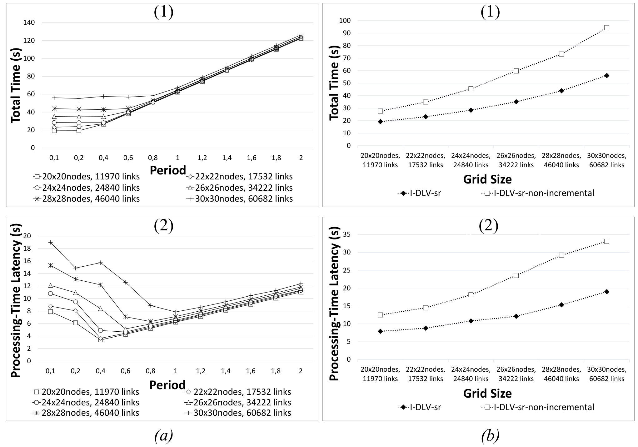
The left column of Figure 4 depicts the results on the Photo-voltaic System benchmark where I-DLV-sr has been tested over different grids with increasing sizes, one size per line. This is a quite expensive domain as rules at lines $2$–$3$ encode a reachability task among working grid panels that vary over time. Plots ($a.1$) and ($a.2$) respectively report total time and latency when on the $x$-axis, the period of incoming requests varies ranging from $0.1$s to $2$s. In this case, #accepted requests is not reported as the system correctly processes all the $60$ requests. As for total time, the six lines in the plot show almost the same trend: constant up to a certain period $P$, and then linearly growing. Note that, for greater grid sizes, also $P$ is greater: this is expected, and can be explained by observing latency in Plot ($a.2$). Indeed, for each line in the plot, latency is smaller when the period is close to its $P$ value beyond which we observe the so-called sustainable throughput [21]. This is because for period values smaller than $P$, I-DLV-sr is asked to process requests that come more often, so it starts to enqueue pending requests. When the period is greater than $P$, instead, I-DLV-sr is able to consider a request as soon as it arrives, thus no queuing is needed, and the greater the period is w.r.t. $P$, the greater it is the idle time between the complete processing of a request and the incoming of the next one. Periods close to $P$ are ideal, as idle time is close to $0$ and no queuing occurs. The right column of Figure 4 compares the performance of two different versions of I-DLV-sr versions: one relies on the incremental $\cal I$²-DLV system, whilst the other relies on the non-incremental $\cal I$-DLV engine (v. 1.1.6). Plots ($b.1$) and ($b.2$) report total time and latency, respectively, of the two tested versions of I-DLV-sr, when on the $x$-axis the grid sizes vary; the period of incoming requests is set to $0.1$s. We observe that the version relying on the incremental evaluator keeps total time and latency smaller than the other; the gap between the two lines becomes more and more evident as the grid size increases, suggesting that I-DLV-sr scales better when relying on the incremental-based version. Intuitively, the gain is attributable to the incremental computation of the transitive closure of the reachable relation over working panels; indeed, the adopted overgrounding technique maintains and reuses all the previously computed ones, rather than recomputing from scratch all the connections. We conclude by mentioning that the same analysis about incrementality has been also done for Content Caching and Heavy Join; however, as these domains are not data-intensive, the evaluation time per rule is so small that recomputing everything from scratch each time is not that expensive. Results (see B) show that the incremental-based version behaves as the non-incremental one without suffering from potential overheads.

Stream Reasoning has been subject of a number of researches over the latest years.Nevertheless, there are no standardized formalisms nor techniques for SR to date, making the comparison among approaches relying on different semantics and technologies rather difficult. Apart several relevant solutions stemmed in the semantic-web context [1, 24, 23, 18], the proposals that relate most with ours are the ones based on ASP. With this respect, one well-established is LARS: Logic for Analytic Reasoning over Streams [5], a formal framework enriching ASP with temporal modalities and window operators. LARS theoretically consists of a full-fledged non-monotonic formalism for reasoning over streams; indeed, the full language is computationally intractable. Current implementations, such as Laser [2], Ticker [6], and its recent distributed version [14], support smaller, yet practically relevant fragments. For performance reasons, Laser handles only negation-stratified and stream-stratified programs, i.e., recursion is not supported if it involves negation or windows [4]. Ticker comes with two evaluation modes: one makes use of the state-of-the-art ASP system clingo [16] as back-end, and is intended for stratified programs, i.e., programs having only a single model; the other mode uses incremental truth maintenance techniques under ASP semantics, and, in case of multiple solutions, computes and maintains one single model randomly chosen. Distributed-SR is an additional version of Ticker, recently released; in order to increase the throughput, it implements an interval-based semantics of LARS that relies on Ticker as internal engine; it supports distributed computation, at the price of disabling the support for recursion through window operators. All Ticker versions require any variable appearing in the scope of a window atom to be “guarded” by some standard atom including it; such variables are grounded upfront in a so-called pre-grounding phase.

I-DLV-sr supports the ASP fragment stratified w.r.t. negation, which is extended with streaming literals over temporal intervals: recursion involving streaming literals is freely allowed as well. The implementation is designed for supporting incremental evaluation of I-DLV-sr programs, thanks to the integration with $\cal I$²-DLV, and parallel/distributed computation, thanks to the integration with Flink. From the one hand, incrementality allows to efficiently evaluate logic programs at each time point and to avoid the need for pre-grounding; also, apart from “canonical” safety, no restriction is required for variables in streaming literals. On the other hand, parallelism and distribution pave the way to the efficient evaluation of streaming atoms. During execution, each operator in the Flink dataflow can have one or more operator subtasks, that are independent from each other; hence, they can be executed in different threads and possibly on different machines or containers. In case of recursive subprograms, distribution is limited by evaluating the involved streaming atoms via single-threaded, undistributed operators.

A distributed stream reasoner that has in common with I-DLV-sr the usage of a stream processor is BigSR [25]; it is released in two versions built on top of the state-of-the-art stream processors Spark Streaming (https://spark.apache.org) and Flink, respectively. BigSR implements internal reasoning algorithms to compute the semantics, and significantly differs from I-DLV-sr on the supported language, the input format and the provided features. In particular, it is oriented towards ontology-based reasoning and accepts RDF input streams. Moreover, input programs fall in the positive fragment of plain LARS and can only contain the in window operator. In addition, depending on the stream processor, further limitations are required. The version relying on Spark Streaming accepts stratified programs that can be recursive but have only global windows, i.e., the rules must share the same window operator. The version built on top of Flink, instead, accepts non-recursive stratified programs, but with global windows at rule scope, i.e., all literals in a rule must share the same window operator. In this latter version, such limitations are due to the BigSR usage of the multi-core/distributed nature of Flink, that makes the handling of synchronization of clocks, task progress and window trigger mechanisms difficult. Furthermore, I-DLV-sr and BigSR differs for the adopted notion of time, as the former relies on event time notion while the latter on the ingestion time one [19].

When designing I-DLV-sr, Spark Streaming and Apache Storm [26] were evaluated as alternative stream processors. Spark Streaming was excluded as, when receiving live input streams, it divides the data into batches, which are lately processed by the Spark engine to generate the final stream in batches. On the other hand, Flink does not require the a-priori creation of batches and works in real-time, record by record, rather than batch by batch. Apache Storm can handle data processing record by record but, it does not provide the event time processing and does not natively offers the exactly-once semantics as instead Flink does. This semantics ensures to I-DLV-sr that each incoming event affects the final outcome exactly once and, even in case of a machine or software failure, there is no data duplication nor unprocessed data.

We presented I-DLV-sr, an ASP-based stream reasoner relying on a tight interaction between $\cal I$²-DLV and a Flink application, that in the experiments showed good performance and scalability. I-DLV-sr is easily extendable by design; hence, we plan to add the support to additional language constructs while extending tests over new real-world domains. Furthermore, we plan to study proper means to extend the language for the management of noise and incompleteness, and further move towards a more complete SR reasoner [12].

References

- Barbieri et al. (2010) Barbieri, D. F., Braga, D., Ceri, S., Valle, E. D., and Grossniklaus, M. 2010. C-SPARQL: a continuous query language for RDF data streams. Int. J. Semantic Comput. 4, 1, 3–25.
- Bazoobandi et al. (2017) Bazoobandi, H. R., Beck, H., and Urbani, J. 2017. Expressive stream reasoning with laser. In International Semantic Web Conference (1). LNCS, vol. 10587. Springer, 87–103.
- Beck et al. (2017) Beck, H., Bierbaumer, B., Dao-Tran, M., Eiter, T., Hellwagner, H., and Schekotihin, K. 2017. Stream reasoning-based control of caching strategies in CCN routers. In IEEE International Conference on Communications, ICC 2017, Paris, France, May 21-25, 2017. IEEE, 1–6.
- Beck et al. (2015) Beck, H., Dao-Tran, M., and Eiter, T. 2015. Answer update for rule-based stream reasoning. In IJCAI. AAAI Press, 2741–2747.
- Beck et al. (2018) Beck, H., Dao-Tran, M., and Eiter, T. 2018. LARS: A logic-based framework for analytic reasoning over streams. Artif. Intell. 261, 16–70.
- Beck et al. (2018) Beck, H., Dao-Tran, M., Eiter, T., and Folie, C. 2018. Stream reasoning with LARS. Künstliche Intell. 32, 2-3, 193–195.
- Brewka et al. (2011) Brewka, G., Eiter, T., and Truszczynski, M. 2011. Answer set programming at a glance. Communications of the ACM 54, 12, 92–103.
- Calimeri et al. (2020) Calimeri, F., Faber, W., Gebser, M., Ianni, G., Kaminski, R., Krennwallner, T., Leone, N., Maratea, M., Ricca, F., and Schaub, T. 2020. Asp-core-2 input language format. TPLP 20, 2, 294–309.
- Calimeri et al. (2017) Calimeri, F., Fuscà, D., Perri, S., and Zangari, J. 2017. I-DLV: the new intelligent grounder of DLV. Intelligenza Artificiale 11, 1, 5–20.
- Calimeri et al. (2019) Calimeri, F., Ianni, G., Pacenza, F., Perri, S., and Zangari, J. 2019. Incremental answer set programming with overgrounding. TPLP 19, 5-6 (Sep), 957–973.
- Carbone et al. (2015) Carbone, P., Katsifodimos, A., Ewen, S., Markl, V., Haridi, S., and Tzoumas, K. 2015. Apache flink™: Stream and batch processing in a single engine. IEEE Data Eng. Bull. 38, 4, 28–38.
- Dell’Aglio et al. (2017) Dell’Aglio, D., Valle, E. D., van Harmelen, F., and Bernstein, A. 2017. Stream reasoning: A survey and outlook. Data Sci. 1, 1-2, 59–83.
- Do et al. (2011) Do, T. M., Loke, S. W., and Liu, F. 2011. Answer set programming for stream reasoning. In Canadian Conference on AI. LNCS, vol. 6657. Springer, 104–109.
- Eiter et al. (2019) Eiter, T., Ogris, P., and Schekotihin, K. 2019. A distributed approach to LARS stream reasoning (system paper). TPLP 19, 5-6, 974–989.
- Gebser et al. (2011) Gebser, M., Grote, T., Kaminski, R., and Schaub, T. 2011. Reactive answer set programming. In LPNMR. LNCS, vol. 6645. Springer, 54–66.
- Gebser et al. (2019) Gebser, M., Kaminski, R., Kaufmann, B., and Schaub, T. 2019. Multi-shot ASP solving with clingo. TPLP 19, 1, 27–82.
- Gebser et al. (2018) Gebser, M., Leone, N., Maratea, M., Perri, S., Ricca, F., and Schaub, T. 2018. Evaluation techniques and systems for answer set programming: a survey. In IJCAI. ijcai.org, 5450–5456.
- Hoeksema and Kotoulas (2011) Hoeksema, J. and Kotoulas, S. 2011. High-performance distributed stream reasoning using s4. In Ordring Workshop at ISWC.
- Hueske and Kalavri (2019) Hueske, F. and Kalavri, V. 2019. Stream Processing with Apache Flink: Fundamentals, Implementation, and Operation of Streaming Applications. O’Reilly Media, Incorporated.
- Ianni et al. (2020) Ianni, G., Pacenza, F., and Zangari, J. 2020. Incremental maintenance of overgrounded logic programs with tailored simplifications. TPLP 20, 5, 719–734.
- Karimov et al. (2018) Karimov, J., Rabl, T., Katsifodimos, A., Samarev, R., Heiskanen, H., and Markl, V. 2018. Benchmarking distributed stream data processing systems. In 34th IEEE International Conference on Data Engineering, ICDE 2018, Paris, France, April 16-19, 2018. IEEE Computer Society, 1507–1518.
- Mileo et al. (2013) Mileo, A., Abdelrahman, A., Policarpio, S., and Hauswirth, M. 2013. Streamrule: A nonmonotonic stream reasoning system for the semantic web. In RR. LNCS, vol. 7994. Springer, 247–252.
- Pham et al. (2019) Pham, T., Ali, M. I., and Mileo, A. 2019. C-ASP: continuous asp-based reasoning over RDF streams. In LPNMR. LNCS, vol. 11481. Springer, 45–50.
- Phuoc et al. (2011) Phuoc, D. L., Dao-Tran, M., Parreira, J. X., and Hauswirth, M. 2011. A native and adaptive approach for unified processing of linked streams and linked data. In International Semantic Web Conference (1). LNCS, vol. 7031. Springer, 370–388.
- Ren et al. (2018) Ren, X., Curé, O., Naacke, H., and Xiao, G. 2018. Bigsr: real-time expressive RDF stream reasoning on modern big data platforms. In IEEE BigData. IEEE, 811–820.
- Toshniwal et al. (2014) Toshniwal, A., Taneja, S., Shukla, A., Ramasamy, K., Patel, J. M., Kulkarni, S., Jackson, J., Gade, K., Fu, M., Donham, J., Bhagat, N., Mittal, S., and Ryaboy, D. V. 2014. Storm@twitter. In SIGMOD Conference. ACM, 147–156.