Learning Linearized Assignment Flows for Image Labeling
Abstract.
We introduce a novel algorithm for estimating optimal parameters of linearized assignment flows for image labeling. An exact formula is derived for the parameter gradient of any loss function that is constrained by the linear system of ODEs determining the linearized assignment flow. We show how to efficiently evaluate this formula using a Krylov subspace and a low-rank approximation. This enables us to perform parameter learning by Riemannian gradient descent in the parameter space, without the need to backpropagate errors or to solve an adjoint equation. Experiments demonstrate that our method performs as good as highly-tuned machine learning software using automatic differentiation. Unlike methods employing automatic differentiation, our approach yields a low-dimensional representation of internal parameters and their dynamics which helps to understand how assignment flows and more generally neural networks work and perform.
Key words and phrases:
assignment flows, image labeling, parameter learning, exponential integration, low-rank approximation2010 Mathematics Subject Classification
34C40, 62H35, 68U10, 68T05, 91A221. Introduction
1.1. Overview, Motivation
Learning the parameters of large neural networks from training data constitutes a basic problem in imaging science, machine learning and other fields. The prevailing approach utilizes gradient descent or approximations thereof based on automatic differentiation [BPRS18] and corresponding software tools, like PyTorch [PGM+19] and TensorFlow [AAB+16]. This kind of software support has been spurring research in imaging science and machine learning dramatically. However, merely relying on numerical schemes and their automatic differentiation tends to thwart attempts to shed light on the often-criticized black-box behavior of deep networks and to better understand the internal representation and function of parameters and their adaptive dynamics.
In this paper, we explore a different route. Adopting the linearized assignment flow approach introduced by [ZSPS20], we focus on a corresponding large system of linear ODEs of the form
| (1.1) |
and study a geometric approach to learning the regularization parameters by Riemannian gradient descent of a loss function
| (1.2) |
constrained by the dynamical system (1.1). Here, we exploit the crucial property that the solution to (1.1) can be specified in closed form (2.24) and can be computed efficiently using exponential integration ([ZSPS20] and Section 2.4). Matrix represents a tangent vector of the so-called assignment manifold, is the number of nodes of the underlying graph, and is the number of labels (classes) that have to be assigned to data observed at nodes . Specifically,
- •
we derive a formula – see Theorem 3.8 – for the Euclidean parameter gradient in closed form;
- •
we show that a low-rank representation of this gradient can be used to efficiently and accurately approximate this closed form gradient; neither backpropagation, nor automatic differentiation or solving adjoint equations are required;
- •
we highlight that the resulting parameter estimation algorithm, in terms of a Riemannian gradient descent iteration (3.7) on the parameter manifold, can be implemented without any specialized software support with modest computational resources;
The significance of our work reported in this paper arises in a broader context. The linearized assignment flow approach also comprises the equation
| (1.3) |
that yields the labeling in terms of almost integral assignment vectors that form the rows of the matrix , depending on the solution of (1.1) for a sufficiently large time . Both equations (1.3) and (1.1) together constitute a linearization of the full nonlinear assignment flow [ÅPSS17]
| (1.4) |
at the barycenter of the assignment manifold. Choosing an arbitrary sequence of time intervals (step sizes) and setting
| (1.5) |
a sequence of linearized assignment flows
| (1.6a) | ||||
| (1.6b) | ||||
| can be computed in order to approximate (1.4) more closely, where solves the corresponding updated ODE (1.1) of the form | ||||
| (1.6c) | ||||
The time-discrete equations (1.6) reveal two basic ingredients of deep networks (or neural ODEs) which the full assignment flow (1.4) embodies in a continuous-time manner: coupling a pointwise nonlinearity (1.6a) and diffusion (1.6b),(1.6c) enhances the expressivity of network models for data analysis.
The key point motivating the work reported in this paper is that our results apply to learning the parameters in each step of the iterative scheme (1.6). We expect that the gradient, and its low-dimensional subspace representations, will help the further study of how each ingredient of (1.6) impacts the predictive power of assignment flows. Furthermore, ‘deep’ extensions of (1.4) and (1.6) are equally feasible within the same mathematical framework (cf. Section 5.2).
1.2. Related Work
Assignment flows were introduced by [ÅPSS17]. For a survey of prior and recent related work, we refer to [Sch20]. Linearized assignment flows were introduced by [ZSPS20] as part of a comprehensive study of numerical schemes for the geometric integration of the assignment flow equation (1.4).
While the bulk of these schemes are based on a Lie group action (cf. [IMKNZ00]) on the assignment manifold, which enables to apply established theory and algorithms for the numerical integration of ODEs that evolve in an Euclidean space [HNW08], the linearity of the ODE (1.1) specifically allows to represent its solution in closed form by the Duhamel (or variation-of-constants) formula [Tes12]. Corresponding extensions to nonlinear ODEs rely on exponential integration [HOS09, HO10]. Iteration (1.6) combines a corresponding iterative scheme and the tangent-space based parametrization (1.3) of the linearized assignment flow.
A key computational step of the latter class of methods requires to evaluate an analytical matrix-valued function, like the matrix exponential and similar functions [Hig08, Section 10]. While basic methods [MVL03] only work for problem of small and medium size, dedicated methods using Krylov subspaces [HL97, AMH11] and established numerical linear algebra [Saa92, Saa03] can be applied to larger problems. The algorithm that results from our approach employs such methods.
Machine learning requires to compute gradients of loss functions that take solutions of ODEs as argument. This defines an enormous computational task and explains why automatic differentiation and corresponding software tools are almost exclusively applied. Alternative dedicated recent methods like [KKRS21] focus on a special problem structure, viz. the action of the differential of the matrix exponential on a rank-one matrix. Our closed form formula for the parameter gradient also involves the differential of a matrix exponential. Yet, we wish to evaluate the gradient itself rather than its action on another matrix. The special problem structure that we can exploit is the Kronecker sum of matrices. Accordingly, our approach is based on the recent corresponding work [BS17] and an additional subsequent low-rank approximation.
1.3. Contribution, Organization
We derive a closed form expression of the gradient of any loss function of the form (1.2) that depends on the solution of the linear system of ODEs (1.1) at some arbitrary but fixed time . In addition, we develop a numerical method that enables to evaluate the gradient efficiently for the common large sizes of image labeling problems. We apply the method to optimal parameter estimation by Riemannian gradient descent and validate our approach by a series of proof-of-concept experiments. This includes a comparison with automatic differentiation applied to two numerical schemes for integrating the linearized assignment flow: geometric explicit Euler and exponential integration. It turns out that our method is as accurate and efficient as the highly optimized automatic differentiation software, like PyTorch [PGM+19] and TensorFlow [AAB+16]. We point out that to our knowledge, automatic differentiation has not been applied to exponential integration, so far.
This paper extends the conference paper [ZPS21] in that all parameter dependencies of the loss function, constrained by the linearized assignment flow, are taken into account (cf. diagram (3.15)). In addition, a complete proof of the corresponding main result (Theorem 3.8) is provided. The space complexity of various gradient approximations are specified in a series of Remarks. The approach is validated numerically and more comprehensively by comparing to automatic differentiation and by examining the influence of all parameters.
The plan for this paper is as follows. Section 2 summarizes the assignment flow approach, the linearized assignment flow and exponential integration for integrating the latter flow. Section 3 details the derivation of the exact gradient of any loss function of the flow with respect to the weight parameters that regularize the flow. Furthermore, a low-rank approximation of the gradient is developed for evaluating the gradient efficiently. We also sketch how automatic derivation is applied to two numerical schemes in order to solve the parameter estimation problem in alternative ways. Numerical experiments are reported in Section 4 for comparing the methods and for inspecting quantitatively the gradient approximation and properties of the estimated weight patches that parametrize the linearized assignment flow. We conclude in Section 5 and point out further directions of research.
2. Preliminaries
2.1. Basic Notation
We set for . The cardinality of a finite set is denoted by , e.g. . denotes the positive orthant and its interior. has dimension depending on the context that we specify sometimes by a subscript, e.g. . Similarly, we set . is the canonical basis of and the identity matrix.
The support of a vector is denoted by . is the probability simplex whose points represent discrete distributions on . Distributions with full support form the relative interior . is the Euclidean inner product of vectors and matrices. In the latter case, this reads with the trace . The induced Frobenius norm is denoted by , and other matrix norms like the spectral norm are indicated by subscripts. The mapping sends a vector to the diagonal matrix with entries . denotes the Kronecker product of matrices and [Gra81, VL00] and the Kronecker sum
| (2.1) |
We have
| (2.2) |
for matrices of compatible dimensions. The operator turns a matrix into the vector by stacking the row vectors. It satisfies
| (2.3) |
The Kronecker product of two vectors and is defined by viewing the vectors as matrices with only one column and applying the definition of Kronecker products for matrices. We have
| (2.4) |
The matrix exponential of a square matrix is given by [Hig08, Ch. 10]
| (2.5) |
denotes the space of all linear bounded mappings from to .
2.2. Assignment Flow
Let be a given undirected graph with vertices indexing data
| (2.6) |
given in a metric space . In this paper, we focus primarily on the application of image labeling in which the graph is a grid graph equipped with a or larger neighborhood at each pixel . The linearized assignment flow and the learning approach in this paper can, however, also be applied to the case of data labeling on arbitrary graphs.
Along with , prototypical data (labels) are given that represent classes . Supervised image labeling denotes the task to assign precisely one prototype to each datum at every vertex in a coherent way, depending on the label assignments in the neighborhoods . These assignments at are represented by probability vectors
| (2.7) |
The set becomes a Riemannian manifold denoted by when endowed with the Fisher-Rao metric . Collecting all assignment vectors as rows defines the strictly positive row-stochastic assignment matrix
| (2.8) |
that we regard as point on the product assignment manifold . Image labeling is accomplished by geometrically integrating the assignment flow solving
| (2.9) |
where and are defined in (2.11b) resp. (2.17). The assignment flow provably converges towards a binary matrix [ZZS21], i.e. , for every and some , which yields the label assignment . In practice, geometric integration is terminated when is -close to an integral point using the entropy criterion from [ÅPSS17], followed by trivial rounding, due to the existence of basins of attraction around each integral point [ZZS21].
We specify the right-hand side of the differential equation in (2.9) — see (2.14) and (2.17) below — and refer to [ÅPSS17, Sch20] for more details and the background. With the tangent space
| (2.10) |
that does not depend on the base point , we define
| (2.11a) | ||||||
| (2.11b) | ||||||
| (2.11c) | ||||||
| (2.11d) | ||||||
| (2.11e) | ||||||
where multiplication, division, exponentiation and apply component-wise to vectors. Corresponding maps
| (2.12) |
in connection with the product manifold (2.8) are defined analogously, and likewise the tangent space
| (2.13) |
and the extension of the orthogonal projection (2.11a) onto , again denoted by . For example, regarding (2.9), with and (or more generally ), we have
| (2.14a) | ||||
| with | ||||
| (2.14b) | ||||
Given data are taken into account as distance vectors
| (2.15) |
and mapped to by
| (2.16) |
where is a user parameter for normalizing the scale of the data. These likelihood vectors represent data terms in conventional variational approaches: Each individual flow , converges to with and in this sense maximizes the local data likelihood.
The vector field defining the assignment flow (2.9) arises through coupling flows for individual pixels through geometric averaging within the neighborhoods , conforming to the underlying Fisher-Rao geometry
| (2.17a) | ||||
| (2.17b) | ||||
The similarity vectors are parametrized by strictly positive weight patches , centered at and indexed by local neighborhoods , that in turn define the weight parameter matrix
| (2.18) |
The matrix comprises all regularization parameters satisfying the latter linear constraints. Flattening these weight patches defines row vectors and, by complementing with , entries of the sparse row vectors of the matrix . Note that the positivity assumption is reflected by the membership . Throughout this paper, we assume that all pixels have neighborhoods of equal size
| (2.19) |
and therefore simply write . These parameters are used in the linearized assignment flow, to be introduced next. We explain a corresponding parameter estimation approach in Section 3 and a parameter predictor in Section 4.4.
2.3. Linearized Assignment Flow
The linearized assignment flow, introduced by [ZSPS20], approximates (2.9) by
| (2.20) |
around any point . In what follows, we only consider the barycenter
| (2.21) |
which is the initial point of (2.9). The differential equation (2.20) is still nonlinear but can be parametrized by a linear ODE on the tangent space
| (2.22a) | ||||
| (2.22b) | ||||
where matrix linearly depends on the parameters of (2.17). The action of on is explicitly given by [ZSPS20, Prop. 4.4]
| (2.23a) | ||||
| (2.23b) | ||||
where is defined by (2.14b) and we took into account (2.21). The linear ODE (2.22b) admits a closed-form solution which in turn enables a different numerical approach (Section 2.4) and a novel approach to parameter learning (Section 3).
2.4. Exponential Integration
The solution to (2.22b) is given by a high-dimensional integral (Duhamel’s formula) whose value in closed form is given by
| (2.24) |
where the entire function is extended to matrix arguments as the limit of an absolutely convergent power series in the matrix space [HJ91, Theorem 6.2.8]. As the matrix is already very large even for medium-sized images, however, it is not feasible in practice to compute in this way. Exponential integration [HL97, NW12], therefore, was used by [ZSPS20] for approximately evaluating (2.24), as sketched next.
Applying the row-stacking operator (2.3) to both sides of (2.22b) and (2.24), respectively, yields with
| (2.25) |
the ODE (2.22b) in the form
| (2.26a) | ||||||
| (2.26b) | ||||||
| (2.26c) | ||||||
where results from
| (2.27a) | ||||
| (2.27b) | ||||
Using the Arnoldi iteration [Saa03] with initial vector , we determine an orthonormal basis of the Krylov space of dimension . As will be validated in Section 4, choosing yields sufficiently accurate approximations of the actions of the matrix exponential and the operator on a vector, respectively, that are given by
| (2.28a) | ||||
| (2.28b) | ||||
The expression results from computing the left-hand side of the relation [Hig08, Section 10.7.4]
| (2.29) |
and extracting the upper-right vector. Since is a small matrix, any standard method [MVL03] can be used for computing the matrix exponential on the left-hand side.
3. Parameter Estimation
Section 3.1 details our approach for learning optimal weight parameters for a given image and ground truth labeling: Riemannian gradient descent is performed with respect to a loss function that depends on the solution of the linearized assignment flow. A closed form expression of this gradient is derived in Section 3.2 along with a low-rank approximation in Section 3.3 that can be computed efficiently. As an alternative and baseline, we outline in Section 3.4 two gradient approximations based on numerical schemes for integrating the linearized assignment flow and automatic differentiation.
3.1. Learning Procedure
Let
| (3.1) |
denote the space of weight parameter matrices that parametrize the similarity mapping (2.17). Due to (2.18) and (2.19), the restrictions are strictly positive probability vectors, as are the assignment vectors defined by (2.7). Therefore, similar to , we consider each as point on a corresponding manifold equipped with the Fisher-Rao metric and — in this sense — regard in (3.1) as corresponding product manifold.
Let denote the ground truth labeling for a given image, and let be a tangent vector such that . Our objective is to determine such that, for some specified time , the vector
| (3.2) |
given by (2.24) and corresponding to the linearized assignment flow, approximates the direction of and hence
| (3.3) |
In this formula the direction of the vector only is relevant, but not its magnitude. A distance function that also satisfies these properties is given by
| (3.4) |
In addition, we consider a regularizer
| (3.5) |
and define the loss function
| (3.6) |
with from (3.2). is determined by the Riemannian gradient descent sequence
| (3.7) |
with step size . Here
| (3.8) |
is the Riemannian gradient with respect to the Fisher-Rao metric. is given by (2.12) and (2.11b) and effectively applies to the restrictions of the row vectors with all remaining components equal to . It remains to compute the Euclidean gradient of the loss function (3.6) which is presented in the subsequent Section 3.2.
3.2. Loss Function Gradient
In Section 3.2.2 we derive a closed form expression for the loss function gradient (Theorem 3.8), after introducing some basic calculus rules for representing and computing differentials of matrix-valued mappings in Section 3.2.1.
3.2.1. Matrix Differentials
Let be a smooth mapping. Using the canonical identification of the tangent spaces of any Euclidean space with itself, we both represent and compute the differential
| (3.9) |
in terms of a vector-valued mapping , which is defined by according to the commutative diagram
| (3.10) |
In formulas, this means that based on the equation
| (3.11) |
we set
| (3.12) |
and hence define and compute the differential (3.9) as matrix-valued mapping
| (3.13) |
The corresponding linear actions on and , respectively, are given by (3.12). We state an auxiliary result required in the next subsection, which also provides a first concrete instance of the general relation (3.12).
Lemma 3.1 (differential of the matrix exponential).
Proof.
The result follows from [Hig08, Thm. 10.13] where columnwise vectorization is used, after rearranging so as to conform to the row-stacking mapping used in this paper. ∎
3.2.2. Closed-Form Gradient Expression
We separate the computation of and the gradient into several operations that were introduced in sections 2 and 3.1. We illustrate their composition and accordingly the process from parameters to a loss in the following flow diagram that refers to quantities in (2.26) and (2.27) related to the linearized assignment flow, after vectorization.
| (3.15) |
In what follows, we traverse this diagram from top-left to bottom-right and collect each partial result by a corresponding lemma or proposition. Theorem 3.8 assembles all results and provides a closed form expression of the loss function gradient . To enhance readability, the proofs of most Lemmata are listed in Appendix A.1.
We focus on mapping (M1) in diagram (3.15).
Lemma 3.2.
The differential of the function
| (3.16) |
and its transpose are given by
| (3.17a) | ||||
| (3.17b) | ||||
with defined by (2.14).
Proof: see Appendix A.1.
Lemma 3.3.
The differential of the function
| (3.18) |
and its transpose are given by
| (3.19a) | ||||
| (3.19b) | ||||
Proof: see Appendix A.1.
We note that should act on a vector . We prefer the more compact and equivalent non-vectorized expression (3.19b).
Lemma 3.4.
Proof: see Appendix A.1.
We focus on the differential of the vector-valued mapping of (3.15) with given by (2.26c). We utilize the fact that analogous to (2.29), the vector
| (3.22a) | ||||
| can be extracted from the last column of the matrix | ||||
| (3.22b) | ||||
By means of relation (3.11), we associate a vector-valued function with the matrix-valued mapping through
| (3.23) |
and record for later that, for any matrix , equation (3.12) implies
| (3.24) |
Lemma 3.5.
The differential of the mapping in (3.22b) is given by
| (3.25) |
Now we are in the position to specify the differential of the solution to the linearized assignment flow with respect to the regularizing weight parameters.
Proposition 3.6.
Proof.
Equation (3.28a) follows directly from equation (2.26c) and Lemma 3.3 makes explicit the second summand on the right-hand side. It remains to compute the first summand. Using (3.22) and the chain rule, we have for any ,
| (3.29a) | ||||
| Applying to both sides which does not change the vector on the left-hand side, yields by (2.3) | ||||
| (3.29b) | ||||
| Applying Lemma 3.1 and (3.24), we obtain | ||||
| (3.29c) | ||||
| (3.29d) | ||||
| and using (2.2) and (3.22b) | ||||
| (3.29e) | ||||
| (3.29f) | ||||
We finally consider the regularizing mapping , defined by (3.5) and corresponding to mapping (M5) in diagram (3.15). Here, we have to take into account the constraints (2.18) imposed on . Accordingly, we define the corresponding set of tangent matrices
| (3.30) |
Lemma 3.7.
The differential of the mapping in (3.5) is given by
| (3.31) |
Proof: see Appendix A.1.
Putting all results together, we state the main result of this section.
Theorem 3.8 (loss function gradient).
3.3. Gradient Approximation
In this section, we discuss the complexity of the evaluation of the loss function gradient as given by (3.33), and we develop a low-rank approximation (3.47) that is computationally feasible and efficient.
3.3.1. Motivation
We reconsider the gradient given by (3.33). The gradient involves the term , given by (3.28), which comprises two summands. We focus on the computationally expensive first summand on the right-hand side of (3.28a) given by (3.28b)-(3.28c), i.e., the term
| (3.34) |
In order to evaluate the corresponding component of based on (3.33b), the matrix is transposed and multiplied with ,
| (3.35a) | ||||
| (3.35b) | ||||
| (3.35c) | ||||
| (3.35d) | ||||
Thus, the matrix-valued function defined by (2.24) has to be evaluates at a Kronecker sum of matrices and then multiplied by a vector. The structure of this expression has the general form
| (3.36) |
where in our case we have
| (3.37a) | ||||
| (3.37b) | ||||
| (3.37c) | ||||
As the following discussions also hold in the general setting (3.36), we derive our gradient approximation in this full generality. Afterwards, we apply our setting to the gradient approximation (3.47). First, we discuss two ways to compute (3.36):
- Direct computation:
-
Compute the Kronecker sum , evaluate the matrix function and multiply the vector . This approach has space and time complexity of at least , with given by (3.37a). The complexity might be even higher depending on how the function is evaluated.
- Krylov subspace approximation:
Remark 3.9 (space complexity).
Consider an image with pixels (), labels (i.e. ) and using bytes per number. Then the direct computation requires to store more than terabytes of data. The Krylov subspace approximation (with ) is significantly cheaper, but still requires to store more than terabytes. Hence both methods are computationally infeasible especially in view of the fact that (3.36) has to be recomputed in every step of the gradient descent procedure (3.7).
3.3.2. An Approximation by Benzi and Simoncini
To reduce the memory footprint, we employ an approximation for computing (3.36), first discussed by Benzi and Simoncini [BS17], and refine it using a new additional approximation in Section 3.3.3. In the following, the notation from Benzi and Simoncini is slightly adapted to our definition (2.1) of the Kronecker sum that differs from Benzi and Simoncini’s definition of the Kronecker sum ().
The approach uses the Arnoldi iteration [Saa03] to determine orthonormal bases , and the corresponding Hessenberg matrices and of the two Krylov subspaces , . The matrices are connected by a standard relation of Krylov subspaces [Hig08, Section 13.2.1],
| (3.38a) | ||||
| (3.38b) | ||||
where , (resp. , ) refer to the entries of the Hessenberg matrices and the orthonormal bases in the next step of the Arnoldi iteration. With these formulas we deduce
| (3.39a) | ||||
| (3.39b) | ||||
| (3.39c) | ||||
Ignoring the last two summands and multiplying by yields the approximation
| (3.40) |
which after applying and multiplying leads to the approximation
| (3.41) |
of the expression (3.36) as proposed by Benzi and Simoncini. We note that, due to the orthonormality of the bases and and their relation to the vectors that generate the subspaces , , the approximation simplifies to
| (3.42a) | ||||
| (3.42b) | ||||
where denotes the first unit vector.
Remark 3.10 (complexity of the approximation (3.42b)).
Computing and storing the matrices , , and has space complexity and a time complexity of [Saa11, p. 132]. Storing the matrices and has complexity . Finally, multiplying the three matrices , and has time complexity and space complexity .
Ignoring negligible terms (recall ), the entire approximation has computational complexity and storage complexity . Compared to the Krylov subspace approximation of (3.36) discussed in the preceding section, this is a reduction of space complexity by a factor .
Consider an image with pixels () and labels as in Remark 3.9. Then the approximation (3.42b) requires to store a bit more than terabytes. While this is a huge improvement compared to the terabytes from the Krylov approximation (see Remark 3.9), using this approximation is still computationally infeasible. This motivates why we introduce below an additional low-rank approximation that yields a computationally feasible and efficient gradient approximation.
3.3.3. Low-Rank Approximation
We consider again the approximation (3.42b)
| (3.43) |
and decompose the matrix using the singular value decomposition (SVD)
| (3.44) |
with and the singular values . As is generally quite small, computing the SVD is neither computationally nor storage-wise expensive. We accordingly rewrite the approximation in the form
| (3.45a) | ||||
| (3.45b) | ||||
| (3.45c) | ||||
Remark 3.11 (space complexity).
While the factorized form (3.45c) is equal to the approximation (3.42b), it requires only a fraction of the storage space: The intermediate results require storing singular values and numbers for each and , and the final approximation has an additional storage requirement of . In total numbers need to be stored.
For a pixels image with labels (see Remark 3.9), storing this approximation requires at most a gigabyte of memory.
In practice, this can be further improved: Numerical experiments show that the singular values decay very rapidly, such that just the first singular value can be used to obtain the gradient approximation
| (3.46) |
Numerical results in Section 4 demonstrate that this approximation is sufficiently accurate.
Remark 3.12 (space complexity).
The term requires to store numbers, i.e. about twice as much storage space as the original image. In total, we need to store numbers. The required storage for the running example (see Remark 3.9) now adds up to less than 500 megabytes.
We conclude this section by returning to our problem using the notation (3.37) and state the proposed low-rank approximation of the loss function gradient. By (3.33), (3.35), (3.37) and (3.46), we have
| (3.47a) | ||||
| where | ||||
| (3.47b) | ||||
| (3.47c) | ||||
| (3.47d) | ||||
Here, the matrices result from the Arnoldi iteration, cf. (3.38), that returns the two Krylov subspaces used to approximate the matrix vector product , with given by (3.37b).
3.4. Computing the Gradient using Automatic Differentiation
An entirely different approach to computing the gradient of the loss function (3.6) is to not use an approximation of the exact gradient given in closed form by (3.8), but to replace the solution to the linearized assignment flow in (3.33b) by an approximation determined by a numerical integration scheme and to compute the exact gradient therefrom. Thus, one replaces a differentiate-then-approximate approach by an approximate-then-differentiate alternative. We numerically compare these two approaches in Section 4.
We sketch the latter alternative. Consider again the loss function (3.6) evaluated at the linearized assignment flow integrated up to time
| (3.48) |
Gradient approximations determined by automatic differentiation depend on what numerical scheme is used. We pick out two basic choices out of a broad range of proper schemes studied in [ZSPS20]. In both cases, we implemented the loss function in PyTorch together with the functions and given by (2.26). Now two approximations can be distinguished depending on how the mappings are implemented.
- Automatic Differentiation based on the explicit Euler scheme:
-
We partition the interval into subintervals with some step size and use the iterative scheme
(3.49) in order to approximate the solution to the linearized assignment flow ODE (2.26a). As the computations only involve basic linear algebra, PyTorch is able to compute the gradient using automatic differentiation.
- Automatic Differentiation based on exponential integration:
-
The second approximation utilizes the numerical integration scheme developed in Section 2.4. Again, only basic operations of linear algebra are involved so that PyTorch can compute the gradient using automatic differentiation. The more special matrix exponential (2.29) is computed by PyTorch using a Taylor polynomial approximation [BBC19].
Both approaches determine an approximation of the Euclidean gradient which we subsequently convert into an approximation of the Riemannian gradient using Equation (3.8).
4. Experiments
In this section, we report and discuss a series of experiments illustrating our novel gradient approximation (3.47) and the applicability of the linearized assignment flow to the image labeling problem.
We start with a discussion of the data generation (Section 4.1) and the general experimental setup (Section 4.2), before discussing properties of the gradient approximation (Section 4.3). In order to illustrate a complete pipeline that can also label previously unseen images, we trained a simple parameter predictor and report its application in Section 4.4.
4.1. Data Generation
As for the experiments, we focused on the image labeling scenarios depicted in Figures 1(a) and 1(b). Each scenario consists of a set containing five pixel images with random Voronoi structure, in order to mimic low-dimensional structure that has to be separated in noisy data from the background. This task occurs frequently in applications and cannot be solved without adaptive regularization.
For the design of the parameter predictor (Section 4.4), we used all patches of five additional unseen images for validation. In all cases we report the mean over all labeled pixels of 5 training and validation images, respectively. In order to test the resilience to noise, we added Gaussian noise to the images. The ground truth labeling is, in both labeling scenarios, given by the noiseless version of the images.
In the first scenario illustrated by Figure 1(a), we want to separate the boundary of the cells (black label) from their interior (white label). The main difficulty here is to preserve the thin line structures even in the presence of image noise. Weight patches with uniform (uninformed) weights average out most of the lines as Figure 1(c) shows.
In the second scenario illustrated by Figure 1(b), we label the Voronoi cells according to their color represented by 8 labels. Due to superimposed noise, a pixelwise local rounding to the nearest label yields about 50% wrongly labeled pixels, see Figure 1(d).


In both cases, Gaussian noise was added. The resulting noisy images are shown in the lower part of either panel (rescaled in the color channels to avoid color clipping). (c) The amount of noise is chosen quite large such that a labeling with uniform (“uninformed non-adaptive”) weights completely destroys the thin line structure in (a). (d) A pixelwise local nearest label assignment yields around 50% wrongly labeled pixels for the labeling scenario depicted in (b). Both of these naive parameter settings indicate the need for a more structured choice of the weight patches, by taking into account local image features in a local spatial neighborhood.
4.2. Experimental Setup
Features and Parametrization. For simplicity, we used the raw image data in a window around each pixel as feature (2.6) for this pixel. Weight patches in the -matrix (2.18) also had the size of pixels in all experiments. While the linearized assignment flow works with arbitrary features and also with larger neighborhood sizes for the weight parameters, the above setup suffices to illustrate and substantiate the contribution of this paper.
Performance measure. All labelings were evaluated on the tangent space of the assignment manifold using the loss function given by (3.4). Since the values of this function are rather abstract, however, we report the percentage of wrongly labeled pixels in all performance plots.
Gradient computation. We evaluated the loss function and approximated its Riemannian gradient in three different ways, as further detailed in Section 4.3, throughout using uniform (uninformed) weight patches as initialization. In particular, other common ways to update the parameters, like Adam or AdaMax [KB17], are possible as well, in conjunction with our approach. Therefore, we also compared gradient approximations based on our approach with the results of automatic differentiation, as implemented by PyTorch [PGM+19].
Parameter prediction. Parameter prediction for labeling novel data relies on the relation of features extracted from training data to corresponding parameters estimated by the Riemannian gradient descent (3.7). For any feature extracted from novel data, the predictor specifies the parameters, to be used for labeling the data by integrating the linearized assignment flow after substituting the predicted parameters. Details are provided in Section 4.4.
4.3. Properties of the Gradient Approximation
In this section, we report results that empirically validate our novel gradient approximation (3.47) by means of parameter estimation for the linearized assignment flow.
First, we compared our gradient approximation with two methods based on automatic differentiation (backpropagation), see also Section 3.4. To this end, we implemented in PyTorch [PGM+19] the simple explicit Euler scheme (3.49) for integrating the linearized assignment flow and computed the gradient of the loss function (3.6) with respect to using automatic differentiation. Similarly, the Krylov subspace approximation (2.28b) of the solution of the linearized assignment flow was implemented in PyTorch. As all involved computations in this approximation are basic linear algebra operations, PyTorch is able to apply automatic differentiation for evaluating the gradient.
These gradients are used for carrying out the gradient descent iteration (3.7) in order to optimize the weight parameters. Figure 4.2 illustrates the comparison of the three approaches. Although they rely on quite different principles, we observe a remarkable comparability of the three approaches with respect to the reduction of the percentage of wrongly labeled pixels per training iteration, for both noisy and noiseless images. In particular, our low-rank approximation based on the closed-form loss function gradient expression is competitive. In view of the minor differences between the curves, we point out that changing hyperparameters, like the step size in the gradient descent or the scale parameter of the regularizer in (3.5), have a greater effect on the training performance than the choice of either of the three approaches. Overall, these results validate the closed form formulas in Section 3.2 and, in particular, Theorem 3.8, and the subsequent low-rank approximation in Section 3.3. We point out, however, that our approach only reveals data-dependent low-dimensional subspaces where the essential parameters of the linearized assignment flow reside.
Next, we compared our gradient approximation to the exact gradient on a per-pixel basis. However, as the exact gradient is computationally infeasible, we used the gradient produced by automatic differentiation of the explicit Euler scheme with a very small step size as surrogate. Figure 3(a) demonstrates the high accuracy of our gradient approximation. A pixelwise illustration of the gradient approximation, at the initial step of the training procedure for adapting the parameters, is provided by Figure 3(b). The set of pixels with non-zero loss function gradient concentrate around the line structure since here weight adaption is required to achieve a proper labeling.
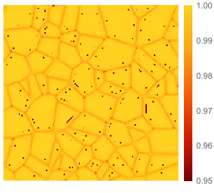

Our last three experiments regarding the gradient approximation, illustrated by Figure 4.4, concern
- •
the influence of the Krylov dimension ,
- •
the rank of our approximation, and
- •
the time up to which the linearized assignment flow is integrated.
We observe according to Figure 4(a) that already Krylov subspace of small dimension suffice for computing linearized assignment flows and learning their parameters. Similarly, the final rank-one gradient approximation of the gradient according to Eq. (3.46) suffices for parameter estimation, as illustrated in Figure 4(b). These experiments show that quite low-dimensional representations suffice for representing the information required for optimal regularization of dynamic image labeling. We point out that such insights cannot be gained from automatic differentiation.
The influence of the time used for integrating the linearized assignment flow on parameter learning is illustrated in Figure 4(c). For the considered parameter estimation setup, we observe that already small integration times yield good training results, whereas large times yield slower convergence. A possible explanation is that, in the latter case, the linearized assignment flow is close to an integral solution which, when erroneous, is more difficult to correct.
4.4. Parameter Prediction
Besides parameter learning, parameter prediction for unseen test data defines another important task. This task amounts to model and represent the relation of local features and optimal weight parameters, as basis to predict proper weights in unseen test data as a function of corresponding local features.
We illustrate this for the scenario depicted by Figure 1(a) using the following simple end-to-end learned approach to parameter prediction. We trained a predictor that produces a weight patch given the features at vertex of novel unseen data. The predictor is parameterized with by
| (4.1a) | feature prototypes, | |||||
| (4.1b) | tangent vectors representing prototypical weight patches, | |||||
and a scale parameter . Similar to the assignment vectors (2.7), the to-be-predicted weight patches are elements of the probability simplex , see (2.18). Accordingly, use tangent vector to represent weight patches. In particular, tangent vector of predicted weight patches result from weight averaging of vectors , and the predicted weight patch by lifting, see (4.4).
We initialize and initialize the by clustering noise-free patches extracted from of training images. Given , we initialize such that it is directed towards the label of the corresponding prototypical patch,
| (4.2) |
The predictor is trained by the following gradient descent iteration. As the change in the number of wrongly labeled pixels was small, we stopped the iteration after steps, see Figure 5(c).
- (1)
We compute the similarities
(4.3) for each and pixels in all training images.
- (2)
We predict the corresponding weight patches as lifted weighted average of the tangent vectors
(4.4) - (3)
Substituting for , we run the linearized assignment flow and evaluate the distance function (3.4).
- (4)
- (5)
The gradient is used to update the predictor parameters, and all steps are repeated.
During training, the accuracy of the predictor is monitored, as illustrated by Figure 5(c). The iteration terminates when the slope of the validation curve, which measures label changes, are sufficiently flat.
After the training of the predictor, the linearized assignment flow is parametrized in a data-driven way so as to separate reliably line structure in noisy data for arbitrary random instances, as depicted by Figure 4.5: panel (f) and last row. This result should be compared to the non-adaptive labeling result in Figure 1(c).


5. Conclusion and Further Work
5.1. Conclusion
We presented a novel approach for learning the parameters of the linearized assignment flow for image labeling. Based on the exact formula of the parameter gradient of a loss function subject to the ODE-constraint, an approximation of the gradient was derived using exponential integration and a Krylov subspace based low-rank approximation, that is memory efficient and sufficiently accurate. Experiments demonstrate that our research implementation is on par with highly tuned-machine learning toolboxes. Unlike the latter, however, our approach additionally returns the essential information for image labeling in terms of a low-dimensional parameter subspace.
5.2. Future Work
Our future work will study generalizations of the linearized assignment flow. Since this can be done within the overall mathematical framework of the assignment flow approach, the result presented in this paper are applicable. We briefly indicate this for the continuous-time ODE (1.1) that we write down here again with an index ,
| (5.1) |
Recall that , given by of (2.22b), represents the input data (2.15) via the mappings (2.16) and (2.17). Now suppose the data are represented in another way and denoted by . Then consider the additional system
| (5.2) |
where the solution to (5.1) at time , possibly transformed to a tangent subspace by a linear mapping , modifies the data term of (5.2). Applying (2.24) to (5.1) at time and to (5.2) at time yields the solution
| (5.3) |
which is a composition of linearized assignment flows and hence linear too, due to the sequential coupling of (5.1) and (5.2). Parallel coupling of the dynamical systems is feasible as well and leads to larger matrix that is structured and linearly depends on the components . Designing larger networks of this sort by repeating these steps is straightforward.
In either case, the overall basic structure of (1.1), (1.3) is preserved. This enables us to broaden the scope of assignment flows for applications and to study, in a controlled manner, various mathematical aspects of deep networks in terms of sequences of generalized linearized assignment flow, analogous to (1.6).
Acknowledgement. This work is funded by the Deutsche Forschungsgemeinschaft (DFG, German Research Foundation) under Germany’s Excellence Strategy EXC 2181/1 - 390900948 (the Heidelberg STRUCTURES Excellence Cluster), and within the DFG priority programme 2298 on the “Theoretical Foundations of Deep Learning”, grant SCHN 457/17-1.
References
- [AAB+16] M. Abadi, A. Agarwal, P. Barham, E. Brevdo, Z. Chen, C. Citro, G. S. Corrado, A. Davis, J. Dean, M. Devin, S. Ghemawat, I. Goodfellow, A. Harp, G. Irving, M. Isard, Y. Jia, R. Jozefowicz, L. Kaiser, M. Kudlur, J. Levenberg, D. Mané, R. Monga, S. Moore, D. Murray, C. Olah, M. Schuster, J. Shlens, B. Steiner, I. Sutskever, K. Talwar, P. Tucker, V. Vanhoucke, V. Vasudevan, F. Viégas, O. Vinyals, P. Warden, M. Wattenberg, M. Wicke, Y. Yu, and X. Zheng, TensorFlow: Large-scale machine learning on heterogeneous systems, OSDI, 2016.
- [AMH11] A. H. Al-Mohy and N. J. Higham, Computing the Action of the Matrix Exponential, with an Application to Exponential Integrators, SIAM Journal on Scientific Computing 33 (2011), no. 2, 488–511.
- [ÅPSS17] F. Åström, S. Petra, B. Schmitzer, and C. Schnörr, Image Labeling by Assignment, Journal of Mathematical Imaging and Vision 58 (2017), no. 2, 211–238.
- [BBC19] P. Bader, S. Blanes, and F. Casas, Computing the Matrix Exponential with an Optimized Taylor Polynomial Approximation, Mathematics 7 (2019), no. 12, 1174.
- [BPRS18] A.G. Baydin, B.A. Pearlmutter, A.A. Radul, and J.M. Siskind, Automatic Differentiation in Machine Learning: a Survey, J. Machine Learning Research 18 (2018), 1–43.
- [BS17] M. Benzi and V. Simoncini, Approximation of Functions of Large Matrices with Kronecker Structure, Numerische Mathematik 135 (2017), no. 1, 1–26.
- [Gra81] A. Graham, Kronecker Products and Matrix Calculus: with Applications, Ellis Horwood Limited, 1981.
- [Hig08] N. J. Higham, Functions of Matrices: Theory and Computation, SIAM, 2008.
- [HJ91] R. A. Horn and C. R. Johnson, Topics in Matrix Analysis, Cambridge University Press, 1991.
- [HL97] M. Hochbruck and C. Lubich, On Krylov Subspace Approximations to the Matrix Exponential Operator, SIAM J. Numer. Anal. 34 (1997), no. 5, 1911–1925.
- [HNW08] E. Hairer, S.P. Nørsett, and G. Wanner, Solving Ordinary Differential Equations I, 3rd ed., Springer, 2008.
- [HO10] M. Hochbruck and A. Ostermann, Exponential integrators, Acta Numerica 19 (2010), 209–286.
- [HOS09] M. Hochbruck, A. Ostermann, and J. Schweitzer, Exponential Rosenbrock-Type Methods, SIAM J. Numer. Anal. 47 (2009), no. 1, 786–803.
- [IMKNZ00] A. Iserles, H. Z. Munthe-Kaas, S. P. Nørsett, and A. Zanna, Lie-Group Methods, Acta Numerica 09 (2000), 215–365.
- [KB17] D. P. Kingma and J. Ba, Adam: A Method for Stochastic Optimization.
- [KKRS21] P. Kandolf, A. Koskela, S. D. Relton, and M. Schweitzer, Computing Low-rank Approximations of the Fréchet Derivative of a Matrix Function Using Krylov Subspace Methods, Numerical Linear Algebra with Applications (2021).
- [MVL03] C. Moler and C. Van Loan, Nineteen Dubious Ways to Compute the Exponential of a Matrix, Twenty-Five Years Later, SIAM Review 45 (2003), no. 1, 3–49.
- [NW12] J. Niesen and W.M. Wright, Algorithm 919: A Krylov Subspace Algorithm for Evaluating the -Functions Appearing in Exponential Integrators, ACM Trans. Math. Software 38 (2012), no. 3, Article 22.
- [PGM+19] A. Paszke, S. Gross, F. Massa, A. Lerer, J. Bradbury, G. Chanan, T. Killeen, Z. Lin, N. Gimelshein, L. Antiga, A. Desmaison, A. Kopf, E. Yang, Z. DeVito, M. Raison, A. Tejani, S. Chilamkurthy, B. Steiner, L. Fang, J. Bai, and S. Chintala, PyTorch: An Imperative Style, High-Performance Deep Learning Library, NIPS, vol. 32, Curran Associates, Inc., 2019.
- [Saa92] Y. Saad, Analysis of Some Krylov Subspace Approximations to the Matrix Exponential Operator, SIAM Journal on Numerical Analysis 29 (1992), no. 1, 209–228.
- [Saa03] by same author, Iterative Methods for Sparse Linear Systems, SIAM, 2003.
- [Saa11] by same author, Numerical Methods for Large Eigenvalue Problems, Classics in Applied Mathematics, Society for Industrial and Applied Mathematics, 2011.
- [Sch20] C. Schnörr, Assignment Flows, Variational Methods for Nonlinear Geometric Data and Applications (P. Grohs, M. Holler, and A. Weinmann, eds.), Springer, 2020, pp. 235–260.
- [Tes12] G. Teschl, Ordinary Differential Equations and Dynamical Systems, Grad. Studies Math., vol. 140, Amer. Math. Soc., 2012.
- [VL00] C. F. Van Loan, The Ubiquitous Kronecker Product, J. Comput. Appl. Math. 123 (2000), 85–100.
- [ZPS21] A. Zeilmann, S. Petra, and C. Schnörr, Learning Linear Assignment Flows for Image Labeling via Exponential Integration, Scale Space and Variational Methods in Computer Vision (SSVM) (A. Elmoataz, J. Fadili, Y. Quéau, J. Rabin, and L. Simon, eds.), LNCS, vol. 12679, 2021, pp. 385–397.
- [ZSPS20] A. Zeilmann, F. Savarino, S. Petra, and C. Schnörr, Geometric Numerical Integration of the Assignment Flow, Inverse Problems 36 (2020), no. 3, 034004 (33pp).
- [ZZS21] A. Zern, A. Zeilmann, and C. Schnörr, Assignment Flows for Data Labeling on Graphs: Convergence and Stability, Information Geometry in press (2021).
Appendix A Proofs
A.1. Proofs of Section 3.2.2
Proof of Lemma 3.2.
Regarding the differential of the mapping (2.11e) with respect to its second argument, we have by [ZSPS20, Lemma 4.5], with given by (2.11b). Applying this relation to (3.16) where acts row-wise analogous to the mapping as explained by (2.12) and (2.14), yields
| (A.1) |
which is (3.17a). As for the transpose, we vectorize both sides using again (2.14),
| (A.2) |
Applying the transposed matrix to any vector with and taking into account the symmetry of the matrix , yields
| (A.3a) | ||||
| (A.3b) | ||||
Proof of Lemma 3.3.
Proof of Lemma 3.4.
We have
| (A.6) |
and have to the differential in the first summand on the right-hand side. By (2.14),
| (A.7) |
and hence is given by
| (A.8) |
It remains to compute and to evaluate the defining right-hand side, to obtain the left-hand side in explicit form. Focusing on a single component of the mapping , we have by (2.11b)
| (A.9a) | ||||
| (A.9b) | ||||
| and hence for any and | ||||
| (A.9c) | ||||
| Thus, analogous to (2.14), we obtain | ||||
| (A.9d) | ||||
| Applying to both sides and comparing with (A.8), we conclude | ||||
| (A.9e) | ||||
which proves (3.21). ∎