Second-order peculiar velocity field as a novel probe of scalar-tensor theories
Abstract
We investigate the galaxy bispectrum induced by the nonlinear gravitational evolution as a possible probe to constrain degenerate higher-order scalar tensor (DHOST) theories. We find that the signal obtained from the leading kernel of second-order density fluctuations is partially hidden by the uncertainty in the nonlinear galaxy bias, and that the kernel of second-order velocity fields instead provides unbiased information on the modification of gravity theory. Based on this fact, we propose new phenomenological time-dependent functions, written as a combination of the coefficients of the second-order kernels, which is expected to trace the higher-order growth history. We then present approximate expressions for these variables in terms of parameters that characterize the DHOST theories. We also show that the resultant formulae provides new constraints on the parameter space of the DHOST theories.
I Introduction
The accelerating cosmic expansion could arise due to a modification of general relativity on cosmological scales. Various theoretical scenarios have been proposed in the literature and should be carefully compared with observational data. Among the cosmological observational data, measuring the growth history of density fluctuations is a powerful tool to test the nature of dark energy and the modification of the theory of gravity responsible for the present cosmic acceleration. In order to efficiently compare the observational data with theoretical predictions, it is convenient to consider phenomenological parameters. A minimal approach to test the theory of gravity from measurements of the growth rate of large-scale structure (LSS) is to introduce the gravitational growth index . This parameter is defined by the logarithmic derivative of the growth rate with respect to the fractional parameter of the non-relativistic matter density as Linder:2007hg
| (1) |
In the standard cosmological model responsible for the present cosmic acceleration, i.e., cold dark matter (CDM) model with general relativity, one shows to be nearly constant at . Although constraints on the growth index have been reported in the literature Grieb:2016uuo; Sanchez:2016sas; Gil-Marin:2018cgo; Zhao:2018gvb, there is no evidence that they deviate from the value predicted by the standard CDM model. Nevertheless, further exploration of the cosmological model landscape requires introducing additional parameters to capture modifications to the theory of gravity.
A possible candidate is a second-order index developed in Yamauchi:2017ibz (see also Namikawa:2018erh). Modifications to the theory of gravity typically alter the clustering properties of LSS. Thus, the quasi-nonlinear growth of LSS can provide new insights into the theory of gravity that would not be imprinted in the growth index of linear perturbation theory. By observing the higher-order correlation function of LSS such as the galaxy bispectrum Gil-Marin:2016wya; Slepian:2016kfz; Pearson:2017wtw; Sugiyama:2018yzo; Sugiyama:2020uil, we can explore the quasi-nonlinear growth of LSS described by the nonlinear kernel of density fluctuations. We define the second-order index as the logarithmic derivative of the time-evolving coefficient in the second-order kernel with respect to as
| (2) |
We expect that second-order indexes can deliver new information on the modification of gravity theories and break the degeneracy between cosmological parameters. Therefore, the purpose of this paper is to revisit the second-order indexes and apply them to a broad class of scalar-tensor gravity theories called degenerate higher-order scalar-tensor theories (DHOST) Langlois:2015cwa; Crisostomi:2016czh; Achour:2016rkg; BenAchour:2016fzp (for a review, see Langlois:2018dxi; Kobayashi:2019hrl). However, as will be shown in the next section, the kernel of the second-order density fluctuation always appears together with the nonlinear galaxy bias functions, making it difficult to directly determine one of the second-order indexes by measuring the galaxy bispectrum. In other words, the features of the second-order indexes are partially hidden by the uncertainty of the nonlinear galaxy bias. To avoid this problem, in this paper, we propose new phenomenological time-dependent functions , and , focusing on the contributions from the second-order peculiar velocity field. We expect that and can be used to constrain modifications to the theory of gravity without any observational uncertainties. In order to compare observational data with theoretical predictions, we develop a formalism describing the evolution equations for the second-order perturbations and derive their explicit expressions as functions of the effective-field-theory (EFT) parameters describing the DHOST theories.
This paper is organized as follows. In Sec. II, we first give the basic equations for the galaxy bispectrum in redshift space and discuss the observational difficulties in the presence of the galaxy nonlinear bias. In Sec. III, following Hirano:2020dom we show the effective Lagrangian describing the DHOST theories and derive the evolution equations for the first- and second-order density fluctuations. We then evaluate the growth index and the second-order index and give their approximate expressions in Sec. IV. We then apply the resultant formulae to the shift-symmetric DHOST cosmology as an application. Finally, Sec. V is devoted to a summary and conclusion.
II Galaxy bispectrum in redshift space
In order to derive the galaxy density fluctuation in redshift space as an observable of galaxy redshift surveys, we first need to describe the matter density field and the peculiar velocity field . For the pressureless nonrelativistic matter, the evolution equation for linear density fluctuations does not depend on the wave number, even when gravity theory is described by a broad class of modified gravity theories, in particular the DHOST theories, as will be discussed later. Hence, the time-dependence of the linear density field can be expressed independently of the wave number, namely , where and denote the linear growth and the initial density fluctuation. On the other hand, the linear velocity divergence field, is written in terms of the logarithmic time derivative of the linear matter density fluctuation through the continuity equation, with . The Fourier transform of the density field and the velocity divergence field are formally expanded in terms of the initial density field as
| (3) | ||||
| (4) |
where is the cosmic scale factor, with dot being the derivative with respect to the cosmic time.
Since the density field is indirectly related to the observables of large-scale structure, the relation between them is needed. We assume that the galaxy density fluctuation up to the second-order can be written as the combination of the linear bias , the second-order bias , and tidal bias (see e.g. Desjacques:2016bnm):
| (5) |
In redshift space, the radial position of galaxies is given by the observed radial component of its relative velocity to an observer. The peculiar velocity field of the underlying matter density distorts the observed position of the galaxy along the line-of-sight. The mapping of a galaxy from its position in real space to its position in redshift space along the line-of-sight direction is expressed as
| (6) |
We then obtain the Fourier component of the galaxy density contrast in redshift space as
| (7) |
Here, the linear- and second-order perturbative kernels are defined as Scoccimarro:1999ed
| (8) | ||||
| (9) |
where , and represents the scale-dependent function corresponding to the tidal force:
| (10) |
Assuming that the initial density field obeys the Gaussian statistics with the power spectrum defined through , the power spectrum and bispectrum of galaxy fluctuations in redshift space at the leading order of perturbation are given by
| (11) | ||||
| (12) |
where .
The modification of gravity theory alters the clustering properties of nonlinear structures and peculiar velocity fields. In particular, the time-dependence of the second-order perturbative kernels and yields a powerful probe of modified gravity theories. In this paper, we only focus on the DHOST theories, while there is a wide variety of gravity theories that yield different signatures to the nonlinear kernels. In the case of the type-I DHOST theories, the second-order kernels can be written in the form Takushima:2013foa; Takushima:2015iha; Crisostomi:2019vhj; Lewandowski:2019txi; Hirano:2020dom:
| (13) | ||||
| (14) |
where and represent the kernel characterizing the second-order mode coupling
| (15) | ||||
| (16) |
Here, when assuming that the matter sector is minimally coupled with gravity, the continuity and Euler equations for the matter give the relation between the coefficients of and kernels as
| (17) | ||||
| (18) |
In the Einstein-de Sitter Universe with general relativity, . In the case of the CDM Universe, one shows , but and deviate slightly from unity, with Bouchet:1994xp; Bernardeau:2001qr; Yamauchi:2017ibz. If the gravity theory is described by the Horndeski scalar-tensor theories Horndeski:1974wa; Deffayet:2011gz; Kobayashi:2011nu, then and still take the standard values, but the time-dependence of and contains information from the underlying theory of gravity Yamauchi:2017ibz; Takushima:2013foa. In the DHOST scalar-tensor theories beyond Horndeski, not only and , but also and can deviate from unity Hirano:2018uar; Crisostomi:2019vhj; Lewandowski:2019txi.
Hereafter, based on these variables let us discuss the degeneracy between the parameters by using the observation data from galaxy redshift surveys. To account for the uncertainty of the amplitude of the power spectrum, it is convenient to introduce as the root-mean-square of the matter fluctuations averaged over . Using this parameter and Eq. (11), one finds that the galaxy power spectrum can only constrain the combinations . In other words, the growth rate measured using the redshift-space distortion (RSD) cannot be independently determined and is always degenerate with by galaxy power spectrum alone. As for the galaxy bispectrum, the situation is slightly changed because the shape dependence should be taken into account. To describe the shape dependence of the galaxy bispectrum induced by the quasi-nonlinear growth, we need to introduce the scale-dependent function related to the shift, which is defined as
| (19) |
in addition to the tidal term Eq. (10) and the scale-independent growth term. Moreover, since the galaxy bispectrum shown in Eq. (12) is in proportion to the square of the matter power spectrum, the term is always measured by the combination with . When taking into account such observational effects, the measured term from the galaxy bispectrum (12) can be rewritten as
| (20) |
From this expression, we found that it is quite challenging to determine one of the coefficients of the second-order kernels, , from the measurement of the galaxy bispectrum, because always appears with the nonlinear galaxy bias functions in the growth and the tidal terms, as shown in the first line of (20). Namely, there is a strong degeneracy between , , and , and the signal of the gravity theory existing in the term would be hidden by the uncertainty of the nonlinear galaxy bias. Moreover, since the shift term in the first line of (20) is measured by the combination of , itself would not be suitable for extracting the information on the modified gravity. On the other hand, as for the term corresponding to the second-order peculiar velocity field, one finds there appear no bias contributions. Hence, we conclude that the second-order peculiar velocity field can be used to constrain the modification of gravity theory without suffering the uncertainty of the galaxy bias.
To avoid the degeneracy between and other parameters related to the modified gravity theory, we propose new parametrizations:
| (21) |
Using these parameters, we expect to easily extract meaningful information for gravity theory from the galaxy bispectrum without suffering from the parameter degeneracy of . Since in the case of general relativity and Horndeski scalar-tensor theories, and can be treated as and inferred from observational data. With these variables, (20) can be rewritten as
| (22) |
This is one of the main results in this paper. Each term in Eq. (22) can be observed independently by taking advantage of the different wave number dependence. Since the linear bias function and the linear growth rate are severely restricted by the observed galaxy power spectrum, we can use the galaxy bispectrum to extract the unbiased information of the parameters , , and from the shift term in the first line, the shift-RSD and the tidal-RSD contributions in the second line of Eq. (22), respectively. As will be shown in the later sections, these three parameters allow us to trace the history of nonlinear growth and encompass the deviations within a broad theoretical framework. In the following section, we present theoretical predictions for the above parameters based on modified gravity theories, specifically the DHOST theories, and demonstrate the implications of these parameters for current and future galaxy redshift surveys.
III Nonlinear gravitational growth in degenerate higher-order scalar-tensor theories
III.1 Small-scale effective theory
In order to describe the perturbations for metric and matter around a spatially flat FLRW solution, it is convenient to use the time-dependent parameters of effective-field-theory (EFT) of dark energy to specify the perturbations fully. For the DHOST theories, these for linear perturbations have been introduced in Langlois:2017mxy and extended to nonlinear order in Dima:2017pwp. In the context of the EFT, the metric is written in the ADM form:
| (23) |
Choosing the time as to coincide with the uniform scalar-field hypersurface, as the perturbed variable, we consider the , the extrinsic curvature the three-dimensional spatial curvature , with . With these variables, the effective Lagrangian is expressed as Langlois:2017mxy; Dima:2017pwp
| (24) |
where , , and . In the EFT language, the degeneracy condition of the type-I DHOST theories to ensure the propagation of a single scalar degree of freedom reduces to
| (25) |
For later convenience, we introduce another time-dependent function:
| (26) |
The minimum set to fully specify the total amount of cosmological perturbations up to the linear order in the type-I DHOST theories is six independent functions of time that are labelled , , , , , and in addition to the Hubble parameter and the effective Planck mass . To take into account the second-order perturbations, we need to consider the additional time-dependent function , which is originally introduced in Yamauchi:2017ibz; Bellini:2015wfa in the context of the Horndeski scalar-tensor theories.
In order to study cosmological perturbations, it is convenient to change the gauge to compare the standard results. To do so, we need to recover the scalar degree of freedom. In this section, we perform a time coordinate transformation and consider the Newtonian gauge given by
| (27) |
We then introduce a dimensionless variable . The nonrelativistic matter energy is given by
| (28) |
To study the quasi-static behaviour deep inside the horizon, we expand the action in terms of the metric and the scalar field perturbations Dima:2017pwp; Kobayashi:2014ida; Hirano:2019scf; Hiramatsu:2020fcd. In the quasi-static regime, the time derivatives of those perturbations are of order Hubble and much smaller than their spatial derivatives. Moreover, the Lagrangian is dominated by terms with spatial derivatives for fields. Namely, we will keep the terms of the form of in the action, where stands for any of , , and their time derivatives. The matter overdensity is assumed to be of . We note that we should keep the mixed derivative terms such as , which cannot be simply ignored, as shown in Kobayashi:2014ida. By expanding the action following the above rule, we obtain the small-scale effective Lagrangian of the form
| (29) |
where denote the -th order terms, which are explicitly given by
| (30) |
and
| (31) |
Here, the explicit forms of and are given
| (32) | ||||
| (33) |
with . The coefficients and the time-dependent functions related to the scalar-tensor theories and should be evaluated on the background.
III.2 Evolution equation for density fluctuations
By varying the Lagrangian with respect to , , and , and solving them in terms of and its time derivatives, we can formally write the effective Poisson equation valid up to the second-order Takushima:2013foa; Takushima:2015iha; Hirano:2020dom
| (34) |
where the second-order mode coupling functions and were defined in Eqs. (15) and (16). Here, the time-dependent functions , , , and are related to the EFT parameters () and appearing in Eq. (24). Their relations are shown in Appendix A.
Throughout this paper, we assume that the matter is minimally coupled to gravity. The continuity and Euler equations for the pressureless nonrelativistic matter are given by
| (35) | ||||
| (36) |
Although these fluid equation are same as the standard ones in general relativity, there appears the effect of the modification of gravity theory through the effective Poisson equation (34). Combining these with Eq. (34) to eliminate the gravitational potential , we derive the closed-form equation for the linear growth of the density fluctuation, , in the form
| (37) |
where , . Once the time-dependent coefficients and are given, one can solve this equation with the boundary condition given by at . This equation can be reinterpreted as the evolution equation for the linear growth rate as
| (38) |
This means that the precise measurement of the linear growth rate from the redshift space distortion can provide the information captured in and . To investigate the second-order nonlinear growth of structure, we need to take into account the nonlinear mode coupling terms as the source term. The equation to solve is written as
| (39) |
where the nonlinear coefficients are given by Hirano:2020dom
| (40) | ||||
| (41) |
Reminding Eqs. (3) and (13), we can rewrite Eq. (39) as the equation of :
| (42) |
The second-order kernels and should coincide with the well-known results in the Einstein-de Sitter Universe in the deep matter-dominated era. Hence, we impose the boundary conditions: and at . This shows that the time-dependent coefficients in the second-order kernel, and , can carry the information not only about and but also about the nonlinear interaction terms and . Given the solutions of and by solving the above evolution equation, we can obtain the second-order coefficients of the peculiar velocity field and from Eqs. (17) and (18).
IV Approximate expression
IV.1 Setup
In this section, we consider the approximate expression of the nonlinear growth functions , , , and in order to derive the analytic formulae of the second-order variables , , and [Eq. (21)] in addition to the linear growth rate. To do so, we need to specify the background expansion history of the Universe. First, we write down the Friedmann and the matter conservation equation in terms of as
| (43) | ||||
| (44) | ||||
| (45) |
where denotes a dark-energy effective equation-of-state parameter for the dark energy component, whose energy density and pressure are defined in terms of the Hubble parameter and effective Planck mass through , .
In order to solve Eqs. (38) and (42) analytically, we assume that the Universe can be well described by the CDM model and the excitation of the scalar field is sufficiently suppressed in the deep matter dominated era, and we focus only on the matter dominated era and the early stage of the dark energy dominated era. During the era of interest, we can treat as a expansion parameter 11 1 In this treatment, we treat as a time variable. However, when one applies our formalism to observational data, the redshift-dependence of would be needed. Our definition of depends on not only the background evolution but also the effective Planck mass running, as seen in Eq. (45). The difference between the standard defined in the CDM Universe with general relativity and ours is discussed in Appendix C. . Hence, the equation-of-state parameter , the EFT parameters () and can be expanded as a series expansion form in terms of as
| (46) | ||||
| (47) | ||||
| (48) |
where , , and are constant parameters, which should be evaluated at the deep matter dominated era. Since the equation-of-motions for the linear- and second-order growth of the density fluctuation Eqs. (37) and (39) at the deep matter dominated era is also assumed to be consistent with the standard one in the CDM model, their deviation should be suppressed by the factor . Therefore, it is expected that the early-time asymptotes of , , , and for are , , , and . These variables during the era of interest can be written as
| (49) | ||||
| (50) | ||||
| (51) | ||||
| (52) |
Here, the first-order coefficients , , , and can be written in terms of the expansion parameters defined in Eqs. (46)–(48). The explicit form of these are presented in Appendix B.
IV.2 First-order
Let us first solve the first order equation (38) to express the growth rate , following Ref. Hirano:2019nkz. Based on the assumption described in the previous subsection, the equation for the growth rate can reduce to
| (53) |
Since the growth rate approaches to unity at the deep matter dominated era, we can solve the above equation to obtain the next-leading order solution of in terms of as
| (54) |
which immediately implies that the corresponding growth index , which was defined in Eq. (1), is given by
| (55) |
Substituting the explicit expressions of [Eq. (143)] and [Eq. (144)] into Eq. (55), we obtain
| (56) |
where
| (57) | ||||
| (58) |
with
| (59) |
IV.3 Second-order
We next derive the solution of the second-order equation-of-motion for the density fluctuation under the assumptions discussed in Sec. IV.1. We can formally solve the equations for the second-order coefficients and , Eq. (42). The corresponding solutions are then written as
| (60) | ||||
| (61) |
The corresponding second-order indexes Eq. (2) are expressed as
| (62) | ||||
| (63) |
With the use of the explicit expression of and given in Eqs. (139) and (151), in addition to , , and , we obtain the approximate solutions of the second-order index and during the matter dominated era and the early stage of the dark energy dominated era. We first show the explicit expression of as
| (64) |
where was defined in Eq. (59), and denotes the leading order solution of the scalar-field perturbation (see Eqs. (112) and (145)), which is explicitly given by
| (65) |
The new parameters and defined in Eq. (21) can be rewritten in terms of and as
| (66) | ||||
| (67) |
which immediately lead to
| (68) | ||||
| (69) |
We found that the nontrivial time-dependence can capture the information of the modification of the gravity theory. An important observation is that in the case of the general relativity and the Horndeski scalar-tensor theories, that is , one can easily show and . Therefore, we conclude that any nonvanishing value of can be treated as the clear signal of the existence of the gravity theory beyond the Horndeski scalar-tensor theories.
Next, let us evaluate in terms of the EFT parameters. We rewrite Eq. (63) by using Eqs. (55), (139), and (143):
| (70) |
The leading term of the nonlinear mode-coupling, , is given by
| (71) |
with
| (72) |
We then translate the second-order index and derived here into the new variable [Eq. (21)]:
| (73) |
Substituting Eqs. (64), (70), and (71) into Eq. (73), can be obtained in terms of constant parameters and , but its explicit expression is complicated. Moreover, the corresponding index can be defined in the same way as through the logarithmic derivative of with respect to . Given the CDM Universe with general relativity, i.e. and , we can reproduce the standard result Bouchet:1994xp; Bernardeau:2001qr, which corresponds to . Unlike , can deviate from the standard value even when . Therefore, we can use the time-dependence of to constrain the Horndeski scalar-tensor theories.
IV.4 Constraining DHOST cosmology with growth and second-order peculiar velocity field
In this subsection, as an application, we apply the resultant formula derived in the previous subsection to the shift-symmetric DHOST model developed in Ref. Hirano:2019nkz. This model allows us to consistently solve the equations for the evolution of both the background and perturbation during the matter-dominated era and the early stage of dark energy-dominated era, and to rewrite the EFT parameters that characterize the DHOST theories in terms of four constant parameters. To proceed with analysis, we focus on the specific type of the DHOST Lagrangian. We assume that the k-essence term in the DHOST theories is in proportion to , where is a constant model parameter. Furthermore, we consider a tracker solution whose scalar field satisfies the condition with being another constant parameter. For instance, in the DHOST cosmological model proposed in Crisostomi:2017pjs, there is a cosmological solution that exhibits the late-time self-acceleration regime, corresponding to the case and . Under these assumptions and considering that the cosmological solution is well described by an attractor solution, the leading order coefficients of the equation-of-state parameter and the braiding parameter are shown to be written in terms of , , , and as
| (74) | ||||
| (75) |
We further consider that the gravitational wave event GW170817 TheLIGOScientific:2017qsa and its optical counterpart GRB170817A Monitor:2017mdv were detected almost simultaneously, providing the stringent constraint on the deviation of the speed of gravitational waves from that of light. This measurement strongly implies that the speed of gravitational waves is in exact agreement with the speed of light. Even with this condition imposed, a certain subclass of type-I DHOST theories survived Langlois:2017dyl; Creminelli:2017sry. The gravitational waves travel at the same speed as light, unaffected by slight changes in the background, when Dima:2017pwp
| (76) |
which corresponds to
| (77) |
When imposing the above conditions, the explicit forms of and in this setup implies the additional relation:
| (78) |
Combining these relations, we finally have independent parameters to model the shift-symmetric DHOST cosmology during the matter dominated era and the early stage of the dark energy dominated era. 22 2 Recently, the constraint from the stability of gravitons against decay into dark energy and the gradient instability induced by gravitational waves are discussed in the literature Creminelli:2018xsv; Creminelli:2019kjy. However, the case with these conditions is shown to be the special class, in which for instance the screening mechanism works only when the parameter fine-tuning is imposed Hirano:2019scf; Crisostomi:2019yfo. Hence, it is beyond the scope of this paper and we simply neglect these possibilities. See also Bahamonde:2019ipm; Bahamonde:2019shr for other possibilities. The growth index , the second-order growth index can be written in terms of as
| (79) | ||||
| (80) |
We can also express in terms of the four constant parameters , while its explicit form is not shown here.
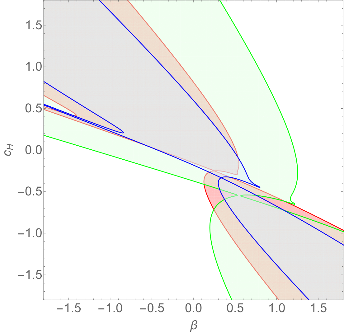
Based on the resultant formulae, we now investigate expected constraints on the DHOST cosmology using current and future observations of large-scale structure. As discussed in Sec. I, the constraints on the growth index from the current observations have been already reported. The typical value of the observational error of the growth index in the current status is roughly estimated as . Therefore, let us employ as a conservative constraint. On the other hand, to the best of our knowledge, no one puts the constraints on , and (or , and ) from observational data. In this paper, as an empirical test, we assume that the error of the second-order indices is . Namely, we consider and . As for , it would be difficult to put a tighter constraint than that of itself, since [see Eq. (66)]. Hence, we focus only on and hereafter. Given the parameter set , we can translate the constraints on using Eqs. (79) and (80).
The parameter regions in the plane allowed by the constraints an for the various values of : (red), (blue), (green) are plotted in Figs. 1 and 2, respectively. These figures show that small changes in the parameters affect the details of the contour of the constant- and constant- curves, though generic features seem to remain unchanged. Hereafter, we focus on the specific parameter set , corresponding to the model proposed in Crisostomi:2017pjs. We show in Fig. 3 the allowed parameter region in the plane obtained from the constraints on the growth index (red), the second-order index (blue) and (green). We found from Fig. 3 that the overlap region, where all these constraints are satisfied, is smaller than the individual allowed region. Therefore, the combined analysis is expected to provide tighter constraints on the DHOST cosmology only from the cosmological observations.
Before closing this section, we briefly discuss present-time observational bounds on the EFT parameters. The Newton potential controls the stellar structure and is characterized by a combination of Dima:2017pwp (See also Langlois:2017dyl for the case after GW170817). The lower bound has been obtained from the existence condition for stars in hydrostatic equilibrium Saito:2015fza, while the upper bound comes from the comparison between the minimum mass of hydrogen-burning stars and the observed minimum red dwarf star Sakstein:2015aac. It is difficult to compare our results directly with these constraints since the leading order expression of , , and are not necessarily valid all the way to the present time. Furthermore, assuming that , , we can compare our results with the present-time bounds.
V Summary
In this paper, we have revisited the galaxy bispectrum as a possible probe to test the theory of gravity beyond linear-order perturbations and have discussed the potential impact of the second-order peculiar velocity field. We have derived the redshift-space galaxy bispectrum with the second-order kernels that include the effect of the modified gravity, and have shown that the signature of the modified gravity obtained from the kernel of the second-order density fluctuations is partially hidden by the uncertainty in the nonlinear galaxy bias functions. We also have pointed out that the contribution from the second-order peculiar velocity field in the galaxy bispectrum can be used to extract the higher-order properties of modified gravity without suffering from the uncertainty of the nonlinear galaxy bias function. Based on this fact, we have proposed the novel phenomenological parameters , and [Eq. (21)] to trace the nonlinear growth history. We then have applied the formulae to the DHOST cosmology and found that the combined analysis of the growth rate and the second-order indices can provide a tight constraint on the DHOST cosmology.
We have developed the formulation of the time evolution for the first- and second-order density fluctuations in the framework of the DHOST theories. By expanding the background and perturbed equations for the density fluctuations in terms of , we have analytically obtained the expression of , and using the parameters that characterize the DHOST theories [Eqs. (69) and (73)], as well as the gravitational growth index [Eq. (56)]. In particular, we have shown that the deviation of from unity can be treated as a clear signal of the gravity theory describing the beyond-Horndeski theories.
Finally, as an application we have applied the resultant expressions to a specific cosmological model of the shift-symmetric DHOST theories, which has the observational constraint on the speed of gravitational waves. We then have obtained the new constraint on the parameter space and found that the analysis combined with the information obtained from , , and provides stringent constraints on the DHOST theories only from cosmological observations.
In this paper, we have considered only the leading term of , , and as the asymptotic values in high redshifts. This assumption is expected to be valid for a wide class of modified gravity theories, and it would be interesting to investigate their time-evolution numerically. In addition, evaluating the galaxy bias function is important for the use of the galaxy bispectrum since the bias function may deviate from that of general relativity due to the modification of gravity theory. The information essentially required to constrain the parameters of and is the anisotropic component of the bispectrum in redshift space, which appears through the second-order velocity field. Therefore, the analysis of the anisotropic component will become more crucial in future bispectrum studies Sugiyama:2018yzo; Sugiyama:2020uil.
Acknowledgements.
We thank Shun Arai, Tomohiro Fujita, Shin’ichi Hirano, and Tsutomu Kobayashi for the fruitful discussion. This work was supported in part by JSPS KAKENHI Grant Nos. 17K14304 (D.Y.), 19H01891 (D.Y.), 19K14703 (N.S.S.).Appendix A Coefficients of first- and second-order solutions
In this Appendix, we briefly review the procedure used in Ref. Hirano:2020dom.
A.1 First-order solutions
To solve the perturbation equations, we first express the variables as a perturbative series:
| (81) |
where denotes the -th order quantities. The equations-of-motion for the first-order and are schematically written as
where and are matrix, which are explicitly defined as
where the index stands for and . Moreover, when varying the effective Lagrangian with respect to , the equation-of-motion for the first-order scalar field perturbation is also schematically written as
| (96) |
The coefficients are given as
| (97) | ||||
| (98) | ||||
| (99) | ||||
| (100) | ||||
| (101) | ||||
| (102) | ||||
| (103) |
Let us solve Eqs. (A.1) and (96) to express , , and in terms of and its time derivatives. Solving Eq. (A.1) for and , and substituting into Eq. (96), one finds that the coefficients of and become zero thanks to the degeneracy condition. Hence, the first-order scalar perturbation can be written in the form
| (104) |
where the coefficients can be written schematically as
| (105) | ||||
| (106) |
The denominator is defined as
| (107) |
Finally, substituting this back into Eq. (A.1), the first-order solutions of the gravitational potentials can be expressed in terms of , , and as
| (108) |
where the coefficients are written in terms of and as well as the components of the matrices and by
| (109) | ||||
| (110) | ||||
| (111) |
A.2 Second-order solutions
At the second-order, we need to take into account the contributions from the nonlinear mode-couplings. To derive the second-order mode-couplings, it would be convenient to introduce the first-order solutions as
| (112) |
Using the coefficients defined in the previous subsection, these can be rewritten as
| (113) | ||||
| (114) | ||||
| (115) | ||||
| (116) |
Then, the equations-of-motion for the second-order variables , , and are schematically written as
| (125) |
where denotes the matrix characterizing the amplitude of the nonlinear mode-couplings for the gravitational potentials, and represents the corresponding coefficient for with representing the scale-dependence of the nonlinear mode-coupling. We have defined as
| (126) |
Since and are generated by the scalar-scalar nonlinear interactions, as clearly seen in the effective Lagrangian Eq. (31), the mode-coupling coefficients can be expressed in terms of the first-order solution of the scalar field perturbation Eq. (112) as
On the other hand, the scalar-gravitational potential nonlinear interactions in addition to the scalar-scalar nonlinear interactions can produce the nonlinear scalar perturbation . Hence, is written as
| (131) | ||||
| (132) |
Substituting the second-order solution of Eq. (A.2) into Eq. (125), the second-order scalar perturbation is expressed in the form
| (133) |
where the coefficients of the nonlinear mode-couplings with the shape are given by
| (134) |
Finally, substituting the solution back into Eq. (A.2), the second-order solutions of the gravitational potentials, are
| (135) |
with
| (136) |
Appendix B Explicit expression for some coefficients
In this Appendix, we summarize some coefficients under the assumptions described in Sec. IV.1. We first expand the time-dependent function defined in Eq. (107) in terms of as
| (137) |
The leading coefficient is given by
| (138) |
Then, the expansion coefficients for , which are defined in Eqs. (109)–(111), are
| (139) | ||||
| (140) | ||||
| (141) |
with
| (142) |
We then obtain the explicit expression of the coefficients in Eqs. (49)–(51) as
| (143) | ||||
| (144) |
To describe the nonlinear mode-coupling terms, we need to expand the first-order solutions Eq. (112) as
| (145) |
which implies that only the first-order scalar field perturbation has the nontrivial zeroth-order contribution. We note from the form of , Eq. (115) that can be well described by the combination of only the coefficients of the first-order equation-of-motion for , Eq. (96), as
| (146) |
The explicit form of the leading order coefficient is given as
| (147) |
Substituting Eqs. (A.2)–(132) into Eq. (134) and expanding it in terms of , we have
| (148) | ||||
| (149) |
with
| (150) |
Then, substituting them into Eq. (136), we finally obtain
| (151) |
and
| (152) |
Appendix C Different parametrization of fractional nonrelativistic matter density
In this paper, we have treated the fractional nonrelativistic matter density as a time variable to evaluate the growth rate and the second-order variables analytically. When comparing our results with actual observational data, we need to evaluate as a function of redshift. However, in the framework of our formulation, it is not easy to solve explicitly. In this section, we discuss a possible prescription for replacing with the one defined in the standard CDM Universe. The fractional energy density in the CDM Universe is defined as
| (153) |
where denotes the Planck mass and is given by the sum of the nonrelativistic matter and the cosmological constant :
| (154) |
During the matter dominated era and the early stage of the dark energy dominated era, , we find that the time-evolution equation (45) can reduce to
| (155) |
We can translate it into the equation for as
| (156) |
We then solve it to obtain
| (157) |
where denotes the initial time. In the case of the CDM Universe, the above expression becomes
| (158) |
Here, we take the deep matter dominated era as the initial time , . At the deep matter dominated era, we assume that the Universe can be well described by the CDM Universe. Namely, . Therefore, the difference between and can be well approximated as
| (159) |
which immediately shows that the difference between and is suppressed by . During the matter dominated era and the early stage of the dark energy dominated era, , the difference is further suppressed by the factor , which is expected to be much smaller than unity. Hence, we expect that can be well approximated by .
References
- (1) E. V. Linder and R. N. Cahn, Astropart. Phys. 28 (2007), 481-488 doi:10.1016/j.astropartphys.2007.09.003 [arXiv:astro-ph/0701317 [astro-ph]].
- (2) J. N. Grieb et al. [BOSS], Mon. Not. Roy. Astron. Soc. 467 (2017) no.2, 2085-2112 doi:10.1093/mnras/stw3384 [arXiv:1607.03143 [astro-ph.CO]].
- (3) A. G. Sanchez et al. [BOSS], Mon. Not. Roy. Astron. Soc. 464 (2017) no.2, 1640-1658 doi:10.1093/mnras/stw2443 [arXiv:1607.03147 [astro-ph.CO]].
- (4) H. Gil-Marín, J. Guy, P. Zarrouk, E. Burtin, C. H. Chuang, W. J. Percival, A. J. Ross, R. Ruggeri, R. Tojerio and G. B. Zhao, et al. Mon. Not. Roy. Astron. Soc. 477 (2018) no.2, 1604-1638 doi:10.1093/mnras/sty453 [arXiv:1801.02689 [astro-ph.CO]].
- (5) G. B. Zhao, Y. Wang, S. Saito, H. Gil-Marín, W. J. Percival, D. Wang, C. H. Chuang, R. Ruggeri, E. M. Mueller and F. Zhu, et al. Mon. Not. Roy. Astron. Soc. 482 (2019) no.3, 3497-3513 doi:10.1093/mnras/sty2845 [arXiv:1801.03043 [astro-ph.CO]].
- (6) D. Yamauchi, S. Yokoyama and H. Tashiro, Phys. Rev. D 96 (2017) no.12, 123516 doi:10.1103/PhysRevD.96.123516 [arXiv:1709.03243 [astro-ph.CO]].
- (7) T. Namikawa, F. R. Bouchet and A. Taruya, Phys. Rev. D 98 (2018) no.4, 043530 doi:10.1103/PhysRevD.98.043530 [arXiv:1805.10567 [astro-ph.CO]].
- (8) H. Gil-Marín, W. J. Percival, L. Verde, J. R. Brownstein, C. H. Chuang, F. S. Kitaura, S. A. Rodríguez-Torres and M. D. Olmstead, Mon. Not. Roy. Astron. Soc. 465 (2017) no.2, 1757-1788 doi:10.1093/mnras/stw2679 [arXiv:1606.00439 [astro-ph.CO]].
- (9) Z. Slepian, D. J. Eisenstein, J. R. Brownstein, C. H. Chuang, H. Gil-Marín, S. Ho, F. S. Kitaura, W. J. Percival, A. J. Ross and G. Rossi, et al. Mon. Not. Roy. Astron. Soc. 469 (2017) no.2, 1738-1751 doi:10.1093/mnras/stx488 [arXiv:1607.06097 [astro-ph.CO]].
- (10) D. W. Pearson and L. Samushia, Mon. Not. Roy. Astron. Soc. 478 (2018) no.4, 4500-4512 doi:10.1093/mnras/sty1266 [arXiv:1712.04970 [astro-ph.CO]].
- (11) N. S. Sugiyama, S. Saito, F. Beutler and H. J. Seo, Mon. Not. Roy. Astron. Soc. 484 (2019) no.1, 364-384 doi:10.1093/mnras/sty3249 [arXiv:1803.02132 [astro-ph.CO]].
- (12) N. S. Sugiyama, S. Saito, F. Beutler and H. J. Seo, Mon. Not. Roy. Astron. Soc. 501 (2021) no.2, 2862-2896 doi:10.1093/mnras/staa3725 [arXiv:2010.06179 [astro-ph.CO]].
- (13) D. Langlois and K. Noui, JCAP 02 (2016), 034 doi:10.1088/1475-7516/2016/02/034 [arXiv:1510.06930 [gr-qc]].
- (14) M. Crisostomi, K. Koyama and G. Tasinato, JCAP 04 (2016), 044 doi:10.1088/1475-7516/2016/04/044 [arXiv:1602.03119 [hep-th]].
- (15) J. Ben Achour, D. Langlois and K. Noui, Phys. Rev. D 93 (2016) no.12, 124005 doi:10.1103/PhysRevD.93.124005 [arXiv:1602.08398 [gr-qc]].
- (16) J. Ben Achour, M. Crisostomi, K. Koyama, D. Langlois, K. Noui and G. Tasinato, JHEP 12 (2016), 100 doi:10.1007/JHEP12(2016)100 [arXiv:1608.08135 [hep-th]].
- (17) D. Langlois, Int. J. Mod. Phys. D 28 (2019) no.05, 1942006 doi:10.1142/S0218271819420069 [arXiv:1811.06271 [gr-qc]].
- (18) T. Kobayashi, Rept. Prog. Phys. 82 (2019) no.8, 086901 doi:10.1088/1361-6633/ab2429 [arXiv:1901.07183 [gr-qc]].
- (19) S. Hirano, T. Kobayashi, D. Yamauchi and S. Yokoyama, Phys. Rev. D 102 (2020) no.10, 103505 doi:10.1103/PhysRevD.102.103505 [arXiv:2008.02798 [gr-qc]].
- (20) V. Desjacques, D. Jeong and F. Schmidt, Phys. Rept. 733 (2018), 1-193 doi:10.1016/j.physrep.2017.12.002 [arXiv:1611.09787 [astro-ph.CO]].
- (21) R. Scoccimarro, H. M. P. Couchman and J. A. Frieman, Astrophys. J. 517 (1999), 531-540 doi:10.1086/307220 [arXiv:astro-ph/9808305 [astro-ph]].
- (22) Y. Takushima, A. Terukina and K. Yamamoto, Phys. Rev. D 89 (2014) no.10, 104007 doi:10.1103/PhysRevD.89.104007 [arXiv:1311.0281 [astro-ph.CO]].
- (23) Y. Takushima, A. Terukina and K. Yamamoto, Phys. Rev. D 92 (2015) no.10, 104033 doi:10.1103/PhysRevD.92.104033 [arXiv:1502.03935 [gr-qc]].
- (24) M. Crisostomi, M. Lewandowski and F. Vernizzi, Phys. Rev. D 101 (2020) no.12, 123501 doi:10.1103/PhysRevD.101.123501 [arXiv:1909.07366 [astro-ph.CO]].
- (25) M. Lewandowski, JCAP 08 (2020), 044 doi:10.1088/1475-7516/2020/08/044 [arXiv:1912.12292 [astro-ph.CO]].
- (26) F. R. Bouchet, S. Colombi, E. Hivon and R. Juszkiewicz, Astron. Astrophys. 296 (1995), 575 [arXiv:astro-ph/9406013 [astro-ph]].
- (27) F. Bernardeau, S. Colombi, E. Gaztanaga and R. Scoccimarro, Phys. Rept. 367 (2002), 1-248 doi:10.1016/S0370-1573(02)00135-7 [arXiv:astro-ph/0112551 [astro-ph]].
- (28) G. W. Horndeski, Int. J. Theor. Phys. 10 (1974), 363-384 doi:10.1007/BF01807638
- (29) C. Deffayet, X. Gao, D. A. Steer and G. Zahariade, Phys. Rev. D 84 (2011), 064039 doi:10.1103/PhysRevD.84.064039 [arXiv:1103.3260 [hep-th]].
- (30) T. Kobayashi, M. Yamaguchi and J. Yokoyama, Prog. Theor. Phys. 126 (2011), 511-529 doi:10.1143/PTP.126.511 [arXiv:1105.5723 [hep-th]].
- (31) S. Hirano, T. Kobayashi, H. Tashiro and S. Yokoyama, Phys. Rev. D 97 (2018) no.10, 103517 doi:10.1103/PhysRevD.97.103517 [arXiv:1801.07885 [astro-ph.CO]].
- (32) D. Langlois, M. Mancarella, K. Noui and F. Vernizzi, JCAP 05 (2017), 033 doi:10.1088/1475-7516/2017/05/033 [arXiv:1703.03797 [hep-th]].
- (33) A. Dima and F. Vernizzi, Phys. Rev. D 97 (2018) no.10, 101302 doi:10.1103/PhysRevD.97.101302 [arXiv:1712.04731 [gr-qc]].
- (34) E. Bellini, R. Jimenez and L. Verde, JCAP 05 (2015), 057 doi:10.1088/1475-7516/2015/05/057 [arXiv:1504.04341 [astro-ph.CO]].
- (35) T. Kobayashi, Y. Watanabe and D. Yamauchi, Phys. Rev. D 91 (2015) no.6, 064013 doi:10.1103/PhysRevD.91.064013 [arXiv:1411.4130 [gr-qc]].
- (36) S. Hirano, T. Kobayashi and D. Yamauchi, Phys. Rev. D 99 (2019) no.10, 104073 doi:10.1103/PhysRevD.99.104073 [arXiv:1903.08399 [gr-qc]].
- (37) T. Hiramatsu and D. Yamauchi, Phys. Rev. D 102 (2020) no.8, 083525 doi:10.1103/PhysRevD.102.083525 [arXiv:2004.09520 [astro-ph.CO]].
- (38) S. Hirano, T. Kobayashi, D. Yamauchi and S. Yokoyama, Phys. Rev. D 99 (2019) no.10, 104051 doi:10.1103/PhysRevD.99.104051 [arXiv:1902.02946 [astro-ph.CO]].
- (39) M. Crisostomi and K. Koyama, Phys. Rev. D 97 (2018) no.8, 084004 doi:10.1103/PhysRevD.97.084004 [arXiv:1712.06556 [astro-ph.CO]].
- (40) B. P. Abbott et al. [LIGO Scientific and Virgo], Phys. Rev. Lett. 119 (2017) no.16, 161101 doi:10.1103/PhysRevLett.119.161101 [arXiv:1710.05832 [gr-qc]].
- (41) B. P. Abbott et al. [LIGO Scientific, Virgo, Fermi-GBM and INTEGRAL], Astrophys. J. Lett. 848 (2017) no.2, L13 doi:10.3847/2041-8213/aa920c [arXiv:1710.05834 [astro-ph.HE]].
- (42) D. Langlois, R. Saito, D. Yamauchi and K. Noui, Phys. Rev. D 97 (2018) no.6, 061501 doi:10.1103/PhysRevD.97.061501 [arXiv:1711.07403 [gr-qc]].
- (43) P. Creminelli and F. Vernizzi, Phys. Rev. Lett. 119 (2017) no.25, 251302 doi:10.1103/PhysRevLett.119.251302 [arXiv:1710.05877 [astro-ph.CO]].
- (44) P. Creminelli, M. Lewandowski, G. Tambalo and F. Vernizzi, JCAP 12 (2018), 025 doi:10.1088/1475-7516/2018/12/025 [arXiv:1809.03484 [astro-ph.CO]].
- (45) P. Creminelli, G. Tambalo, F. Vernizzi and V. Yingcharoenrat, JCAP 05 (2020), 002 doi:10.1088/1475-7516/2020/05/002 [arXiv:1910.14035 [gr-qc]].
- (46) M. Crisostomi, M. Lewandowski and F. Vernizzi, Phys. Rev. D 100 (2019) no.2, 024025 doi:10.1103/PhysRevD.100.024025 [arXiv:1903.11591 [gr-qc]].
- (47) S. Bahamonde, K. F. Dialektopoulos, V. Gakis and J. Levi Said, Phys. Rev. D 101 (2020) no.8, 084060 doi:10.1103/PhysRevD.101.084060 [arXiv:1907.10057 [gr-qc]].
- (48) S. Bahamonde, K. F. Dialektopoulos and J. Levi Said, Phys. Rev. D 100 (2019) no.6, 064018 doi:10.1103/PhysRevD.100.064018 [arXiv:1904.10791 [gr-qc]].
- (49) R. Saito, D. Yamauchi, S. Mizuno, J. Gleyzes and D. Langlois, JCAP 06 (2015), 008 doi:10.1088/1475-7516/2015/06/008 [arXiv:1503.01448 [gr-qc]].
- (50) J. Sakstein, Phys. Rev. D 92 (2015), 124045 doi:10.1103/PhysRevD.92.124045 [arXiv:1511.01685 [astro-ph.CO]].