TOI-431/HIP 26013: a super-Earth and a sub-Neptune transiting a bright, early K dwarf, with a third RV planet2020TOI-431/HIP 26013: a super-Earth and a sub-Neptune transiting a bright, early K dwarf, with a third RV planet–D
Abstract
We present the bright (V), multi-planet system TOI-431, characterised with photometry and radial velocities. We estimate the stellar rotation period to be days using archival photometry and radial velocities. TOI-431 b is a super-Earth with a period of 0.49 days, a radius of 1.28 0.04 R⊕, a mass of M⊕, and a density of g cm-3; TOI-431 d is a sub-Neptune with a period of 12.46 days, a radius of R⊕, a mass of M⊕, and a density of g cm-3. We find a third planet, TOI-431 c, in the HARPS radial velocity data, but it is not seen to transit in the TESS light curves. It has an of M⊕, and a period of 4.85 days. TOI-431 d likely has an extended atmosphere and is one of the most well-suited TESS discoveries for atmospheric characterisation, while the super-Earth TOI-431 b may be a stripped core. These planets straddle the radius gap, presenting an interesting case-study for atmospheric evolution, and TOI-431 b is a prime TESS discovery for the study of rocky planet phase curves.
Keywords:
planets and satellites: individual: (TOI-431, TIC 31374837) – planets and satellites: detection – planets and satellites: fundamental parameters1 Introduction
The discoveries of the Kepler Space Telescope (Borucki et al. 2010) provided us with the means to make statistical studies on the exoplanet population for the first time: Kepler has shown us that Neptune-sized planets are more common than large gas giants (Fressin et al. 2013), and that super-Earths are the most abundant planet type (Petigura et al. 2013). It became possible to look for trends that might elucidate planetary formation mechanisms; one such trend discovered is a bi-modality in the radius distribution of small planets. Often dubbed the “photoevaporation valley,” the commonly posited explanation for its existence is photoevaporation of close-in planetary atmospheres (Owen & Wu 2017; Fulton et al. 2017; Fulton & Petigura 2018; Van Eylen et al. 2018; Cloutier & Menou 2020). Planets above the radius gap have retained gaseous envelopes, while planets below are theorised to have been stripped of any gas to become naked cores. Multi-planet systems have been discovered containing planets that lie both below and above the radius gap (Günther et al. 2019; Cloutier et al. 2020a, e.g.), and such systems are important when considering how evolution mechanisms may sculpt the radius gap as they allow testing of atmospheric evaporation and bulk composition models.
Further to the discovery of the radius gap, a paucity of intermediate-sized planets at short periods ( 3 days) dubbed the “Neptune/sub-Jovian Desert” (Szabó & Kiss 2011; Beaugé & Nesvorný 2013; Helled et al. 2016; Lundkvist et al. 2016; Mazeh et al. 2016; Owen & Lai 2018), can be seen in both the mass-period and radius-period distribution of exoplanets, and Mazeh et al. 2016 and Owen & Lai 2018 derived boundaries for this triangular-shaped region, and the potential mechanisms behind their existence.
The Transiting Exoplanet Survey Satellite (Ricker et al. 2015, TESS,) is now building upon the legacy of Kepler. Unlike Kepler, TESS has been optimised to look at bright stars, enabling high precision radial velocity follow up of planetary candidates to determine their masses, and additional follow-up (with the James Webb Space Telescope, JWST, for example) will allow us to study their atmospheres. Over the course of its two year primary mission, which came to an end in July 2020, over 2000 TESS Objects of Interest (TOIs) were released, and there have been many discoveries that contribute to fulfilling its Level-1 mission goal to measure the masses and radii of at least 50 planets with radii smaller than 4 R⊕ (Huang et al. 2018; Gandolfi et al. 2018; Cloutier et al. 2019; Dragomir et al. 2019; Dumusque et al. 2019; Luque et al. 2019; Díaz et al. 2020; Astudillo-Defru et al. 2020; Cloutier et al. 2020b; Cloutier et al. 2020a; Nielsen et al. 2020; Armstrong et al. 2020, e.g.).
We present here the discovery of TOI-431 b, c, and d. TOI-431 b and d are a super-Earth and sub-Neptune respectively, discovered first by TESS and confirmed via extensive follow up: high-precision Doppler spectroscopy from the High Accuracy Radial velocity Planet Searcher (Pepe et al. 2002, HARPS,) and the HIgh REsolution Spectrograph (Vogt et al. 1994, HIRES,) which allows us to determine their masses; additional Doppler spectroscopy from iSHELL (Rayner et al. 2016a), FEROS (Kaufer & Pasquini 1998), and Minerva-Australis (Addison et al. 2019a); ground-based transit detections from NGTS (Wheatley et al. 2018) and the LCOGT 1m network (Brown et al. 2013); and a double-transit from the Spitzer space telescope. Both TOI-431 b and d contribute to the TESS Level-1 mission goal. TOI-431 c is an additional planet that we have found in the HARPS radial velocity data, and it is not seen to transit. We describe the observations made and the stellar analysis of the TOI-431 system in Section 2; our joint-fit model of the system in Section 3; and put this system into context in Section 4.
2 Observations
| Property | Value | Source |
|---|---|---|
| Identifiers | ||
| TIC ID | 31374837 | TICv8 |
| HIP ID | 26013 | |
| 2MASS ID | 05330459-2643286 | 2MASS |
| Gaia ID | 2908664557091200768 | GAIA EDR3 |
| Astrometric properties | ||
| R.A. (J2016.0) | 05:33:04.62 | GAIA EDR3 |
| Dec (J2016.0) | -26:43:25.86 | GAIA EDR3 |
| Parallax (mas) | 30.65 0.01 | GAIA EDR3 |
| Distance (pc) | 32.61 0.01 | Bailer-Jones et al. 2021 |
| (mas yr-1) | 16.89 0.01 | GAIA EDR3 |
| (mas yr-1) | 150.78 0.01 | GAIA EDR3 |
| Photometric properties | ||
| TESS (mag) | 8.171 0.006 | TICv8 |
| B (mag) | 10.10 0.03 | TICv8 |
| V (mag) | 9.12 0.03 | TICv8 |
| G (mag) | 8.7987 0.0003 | GAIA EDR3 |
| J (mag) | 7.31 0.03 | 2MASS |
| H (mag) | 6.85 0.03 | 2MASS |
| K (mag) | 6.72 0.02 | 2MASS |
- •
Sources: TICv8 (Stassun et al. 2019), 2MASS (Skrutskie et al. 2006), Gaia Early Data Release 3 (Gaia Collaboration et al. 2021)
2.1 Photometry
2.1.1 TESS photometry
The TOI-431 system (TIC 31374837, HIP 26013) was observed in TESS Sectors 5 (Nov 15 to Dec 11 2018) and 6 (Dec 15 2018 to Jan 6 2019) on Camera 2 in the 2-minute cadence mode ( min). TOI-431.01 (now TOI-431 d) was flagged on Feb 8 2019 by the MIT Quick-Look Pipeline (Huang et al. 2019, QLP,) with a signal-to-noise ratio (SNR) of 58; the Sector 5 light curve reveals 2 deep transits of TOI-431 d, but further transits of this planet fell in the data gaps in S6. TOI-431 d passed all Data Validation tests (Twicken et al. 2018, see) and model fitting (Li et al. 2019, see); additionally, the difference image centroiding results place the transit signature source within arcsec of the target star. TOI-431.02 (now TOI-431 b) was flagged later, on June 6, after identification by the TESS Science Processing Operations Center (SPOC) pipeline (Jenkins et al. 2016) with an SNR of 24 in a combined transit search of Sectors 5-6.
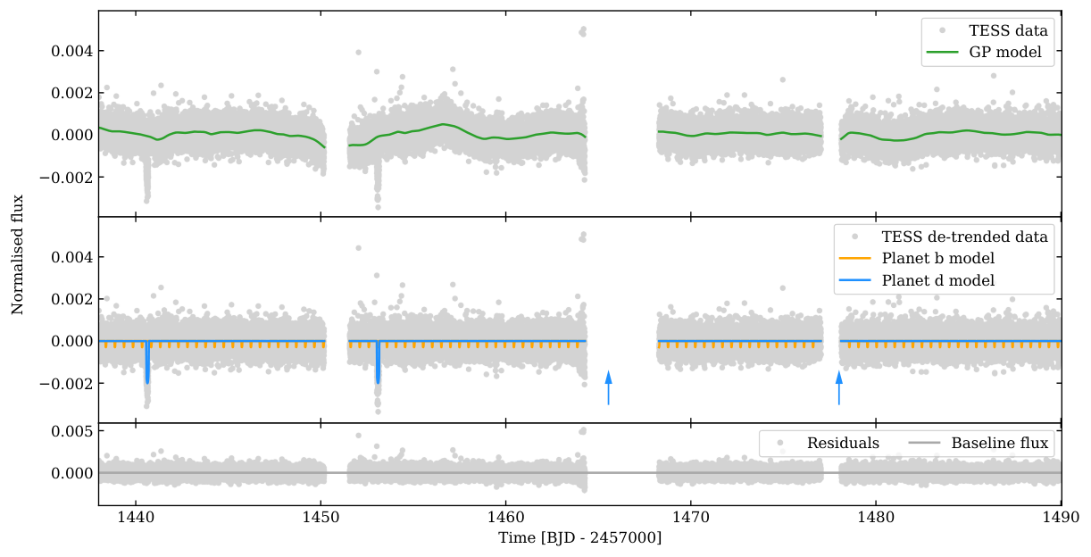
We used the publicly available photometry provided by the SPOC pipeline, and used the Presearch Data Conditioning Simple Aperture Photometry (PDCSAP_FLUX), which has common trends and artefacts removed by the SPOC Presearch Data Conditioning (PDC) algorithm (Twicken et al. 2010; Smith et al. 2012; Stumpe et al. 2012; Stumpe et al. 2014). The median-normalised PDCSAP flux, without any further detrending, is shown in the top panel of Fig. 5.
2.1.2 LCOGT photometry
To confirm the transit timing and depth, and to rule out a nearby eclipsing binary (NEB) as the source of the TESS transit events, we obtained three seeing-limited transit observations of TOI-431 d in the -band. The light curves were obtained using the 1-m telescopes at the Cerro Tololo Inter-American Observatory (CTIO) and the Siding Springs Observatory (SSO) as part of the Las Cumbres Observatory Global Telescope network (Brown et al. 2013, LCOGT;). Both telescopes are equipped with a Sinistro camera with a fine pixel scale of pixel-1.
We calibrated each sequence of images using the standard LCOGT BANZAI pipeline (McCully et al. 2018). The observations were scheduled using the TESS Transit Finder, a customised version of the Tapir software package (Jensen 2013). The differential light curves of TOI-431, and seven neighbouring sources within based on the Gaia DR2 (Gaia Collaboration et al. 2018), were derived from uncontaminated apertures using AstroImageJ (Collins et al. 2017, AIJ;). Two partial transits were obtained on UT December 9 2019 which covered the ingress and egress events from CTIO and SSO respectively (Figure 7). We then obtained a second ingress observation on January 3 2020 from CTIO. Within each light curve, we detected the partial transit event on-target and cleared the field of NEBs down to mag.
2.1.3 PEST photometry
We also obtained a seeing-limited observation during the time of transit of TOI-431 d on UT February 13 2020 using the Perth Exoplanet Survey Telescope (PEST) near Perth, Australia. The 0.3 m telescope is equipped with a SBIG ST-8XME camera with an image scale of 12 pixel-1, resulting in a field of view. A custom pipeline based on C-Munipack11 1 http://c-munipack.sourceforge.net was used to calibrate the images and extract the differential photometry, using an aperture with radius 62. The images have typical stellar point spread functions (PSFs) with a FWHM of . Because the transit depth of TOI-431 d is too shallow to detect from the ground with PEST, the target star was intentionally saturated to check the fainter nearby stars for possible NEBs that could be blended in the TESS aperture. The data rule out NEBs in all 17 stars within of the target star that are bright enough (TESS magnitude < 17.4) to cause the TESS detection of TOI-431 d.
2.1.4 Spitzer photometry
Shortly after TOI-431 was identified and announced as a TESS planet candidate, we identified TOI-431 d as an especially interesting target for atmospheric characterization via transmission spectroscopy. We therefore scheduled one transit observation with the Spitzer Space Telescope to further refine the transit ephemeris and allow efficient scheduling of future planetary transits. We observed the system as part of Spitzer GO 14084 (Crossfield et al. 2018) using the 4.5m channel of the IRAC instrument (Fazio et al. 2004). We observed in subarray mode, which acquired 985 sets of 64 subarray frames, each with 0.4 s integration time. These transit observations spanned UT times from May 23 2019 21:13 to May 24 2019 04:42, and were preceded and followed by shorter integrations observed off-target to check for bad or hot pixels. Our transit observations used Spitzer/IRAC in PCRS Peak-up mode to place the star as closely as possible to the well-characterized “sweet spot” on the IRAC2 detector.
2.1.5 NGTS photometry
The Next Generation Transit Survey (Wheatley et al. 2018, NGTS;) is an exoplanet hunting facility which consists of twelve 20 cm diameter robotic telescopes and is situated at ESO’s Paranal Observatory. Each NGTS telescope has a wide field-of-view of 8 square degrees and a plate scale of 5 arcsec pixel-1. NGTS observations are also afforded sub-pixel level guiding through the DONUTS auto-guiding algorithm (McCormac et al. 2013). A transit event of TOI-431 d was observed using 5 NGTS telescopes on February 20 2020. On this night, a total of 5922 images were taken across the 5 telescopes, with each telescope observing with the custom NGTS filter and an exposure time of 10 seconds. The dominant photometric noise sources in NGTS light curves of bright stars are Gaussian and uncorrelated between the individual telescope systems (Smith et al. 2020; Bryant et al. 2020). As such, we can use simultaneous observations with multiple NGTS telescopes to obtain high precision light curves.
All the NGTS data for TOI-431 were reduced using a custom aperture photometry pipeline which uses the SEP library for both source extraction and photometry (Bertin & Arnouts 1996; Barbary 2016). Bias, dark and flat field image corrections are found to not improve the photometric precision achieved, and so we do not apply these corrections during the image reduction. SEP and GAIA (Gaia Collaboration et al. 2016; Gaia Collaboration et al. 2018) are both used to identify and rank comparison stars in terms of their brightness, colour, and CCD position relative to TOI-431 (Bryant et al. 2020, for more details on the photometry, see).
2.2 Spectroscopy
2.2.1 HARPS high-resolution spectroscopy
TOI-431 was observed between February 2 and October 21 2019 with the High Accuracy Radial velocity Planet Searcher (HARPS) spectrograph mounted on the ESO 3.6 m telescope at the La Silla Observatory in Chile (Pepe et al. 2002). A total of 124 spectra were obtained under the NCORES large programme (ID 1102.C-0249, PI: Armstrong). The instrument (with resolving power ) was used in high-accuracy mode (HAM), with an exposure time of 900 s. Between 1 and 3 observations of the star were made per night. The standard offline HARPS data reduction pipeline was used to reduce the data, and a K5 template was used in a weighted cross-correlation function (CCF) to determine the radial velocities (RVs). Each epoch has further calculation of the bisector span (BIS), full-width at half-maximum (FWHM), and contrast of the CCF. This data is presented in Table 6.
In addition to this, there are 50 publicly available archival HARPS spectra dating from 2004 to 2015.
2.2.2 HIRES high-resolution spectroscopy
We obtained 28 high-resolution spectra of TOI-431 on the High Resolution Echelle Spectrometer of the 10m Keck I telescope (Vogt et al. 1994, Keck/HIRES,). The observation spans a temporal baseline from November 11 2019 to September 27 2020. We obtained an iodine-free spectrum on November 8 2019 as the template for radial velocity extraction. All other spectra were obtained with the iodine cell in the light path for wavelength calibration and line profile modeling. Each of these spectra were exposed for 4-8 min achieving a median SNR of 200 per reduced pixel near 5500 Å. The spectra were analyzed with the forward-modelling Doppler pipeline described in Howard et al. 2010 for RV extraction. We analyzed the Ca II H & K lines and extracted the using the method of Isaacson & Fischer 2010. This data is presented in Table 7.
2.2.3 iSHELL spectroscopy
We obtained 108 spectra of TOI-431 during 11 nights with the iSHELL spectrometer on the NASA Infrared Telescope Facility (Rayner et al. 2016b, IRTF,), spanning 108 days from September-December 2019 . The exposure times were 5 minutes, repeated 3-14 times within a night to reach a cumulative photon signal-to-noise ratio per spectral pixel varying from 131–334 at m (the approximate centre of the blaze for the middle order). This achieves a per-night RV precision of 3–8 ms-1 with a median of 5 ms-1. Spectra were reduced and RVs extracted using the methods outlined in Cale et al. 2019.
2.2.4 FEROS spectroscopy
TOI-431 was monitored with the Fiberfed Extended Range Optical Spectrograph (Kaufer et al. 1999, FEROS,), installed on the MPG2.2 m telescope at La Silla Observatory, Chile. These observations were obtained in the context of the Warm gIaNts with tEss (WINE) collaboration, which focuses on the systematic characterization of TESS transiting warm giant planets (Brahm et al. 2019; Jordán et al. 2020, e.g.,). FEROS has a spectral resolution of R and uses a comparison fibre that can be pointed to the background sky or illuminated by a Thorium-Argon lamp simultaneously with the execution of the science exposure. We obtained 10 spectra of TOI-431 between February 28 and March 12 2020. We used the simultaneous calibration technique to trace instrumental radial velocity variations, and adopted an exposure time of 300 s, which translated in spectra with a typical signal-to-noise ratio per resolution element of 170. FEROS data was processed with the ceres pipeline (Brahm et al. 2017), which delivers precision radial velocity and line bisector span measurements through the cross-correlation technique. The cross-correlation was executed with a binary mask reassembling the properties of a G2-type dwarf star.
2.2.5 Minerva-Australis spectroscopy
Minerva-Australis is an array of four PlaneWave CDK700 telescopes located in Queensland, Australia, fully dedicated to the precise radial-velocity follow-up of TESS candidates. The four telescopes can be simultaneously fiber-fed to a single KiwiSpec R4-100 high-resolution (R=80,000) spectrograph (Barnes et al. 2012; Addison et al. 2019b; Addison et al. 2020). TOI-431 was observed by Minerva-Australis in its early operations, with a single telescope, for 16 epochs between 2019 Feb 12 and 2019 April 17. Each epoch consists of two 30-minute exposures, and the resulting radial velocities are binned to a single point. Radial velocities for the observations are derived for each telescope by cross-correlation, where the template being matched is the mean spectrum of each telescope. The instrumental variations are corrected by using simultaneous Thorium-Argon arc lamp observations.
2.3 High resolution imaging

High angular resolution imaging is needed to search for nearby sources that can contaminate the TESS photometry, resulting in an underestimated planetary radius, or that can be the source of astrophysical false positives, such as background eclipsing binaries. The contrast curves from all of the sources of high resolution imaging described below are displayed in Fig. 1.
2.3.1 SOAR HRCam
We searched for stellar companions to TOI-431 with speckle imaging with the 4.1-m Southern Astrophysical Research (SOAR) telescope (Tokovinin 2018) on UT March 17 2019, observing in the Cousins I-band, a similar visible bandpass to TESS. More details of the observation are available in Ziegler et al. 2020. The 5 detection sensitivity and speckle auto-correlation functions from the observations are shown in Fig. 1. No nearby stars were detected within 3″of TOI-431 in the SOAR observations.
2.3.2 Gemini NIRI
We collected high resolution adaptive optics observations using the Gemini/NIRI instrument (Hodapp et al. 2003) on UT March 18 2019. We collected nine images in the Br filter, with exposure time 0.6 s per image. We dithered the telescope by 2” between each exposure, allowing for a sky background to be constructed from the science frames themselves. We corrected individual frames for bad pixels, subtracted the sky background, and flat-corrected frames, and then co-added the stack of images with the stellar position aligned. To calculate the sensitivity of these observations, we inject fake companions and measure their S/N, and scale the brightness of these fake companions until they are recovered at 5. This is repeated at a number of locations in the image. We average our sensitivity over position angle, and show the sensitivity as a function of radius in Fig. 1. Our observations are sensitive to companions 4.6 mag fainter than the host at 0.2”, and 8.1 mag fainter than the host in the background limited regime, at separations greater than 1”.
2.3.3 Gemini ’Alopeke
TOI-431 was observed on UT Oct 15 2019 using the ‘Alopeke speckle instrument on Gemini-North22 2 https://www.gemini.edu/sciops/instruments/alopeke-zorro/. ‘Alopeke provides simultaneous speckle imaging in two bands, 562 nm and 832 nm, with output data products including a reconstructed image, and robust limits on companion detections (Howell et al. 2011). Fig. 1 shows our results in both 562 nm and 832 nm filters. Fig. 1 (right) shows the 832 nm reconstructed speckle image from which we find that TOI-431 is a single star with no companion brighter than within 5-8 magnitudes of TOI-431 detected within 1.2 ″. The inner working angle of the ‘Alopeke observations are 17 mas at 562 nm and 28 mas at 832 nm.
2.3.4 Keck NIRC2
As part of our standard process for validating transiting exoplanets to assess the possible contamination of bound or unbound companions on the derived planetary radii (Ciardi et al. 2015), we observed TOI-431 with infrared high-resolution Adaptive Optics (AO) imaging at Keck Observatory. The Keck Observatory observations were made with the NIRC2 instrument on Keck-II behind the natural guide star AO system. The observations were made on UT March 25 2019 in the standard 3-point dither pattern that is used with NIRC2 to avoid the left lower quadrant of the detector, which is typically noisier than the other three quadrants. The dither pattern step size was and was performed three times.
The observations were made in the filter m) with an integration time of 1 second and 20 coadds per frame for a total of 300 seconds on target. The camera was in the narrow-angle mode with a full field of view of and a pixel scale of per pixel. The Keck AO observations revealed no additional stellar companions detected to within a resolution FWHM (Fig. 1).
The sensitivities of the final combined AO image were determined by injecting simulated sources azimuthally around the primary target every at separations of integer multiples of the central source’s FWHM (Furlan et al. 2017). The brightness of each injected source was scaled until standard aperture photometry detected it with significance. The resulting brightness of the injected sources relative to the target set the contrast limits at that injection location. The final limit at each separation was determined from the average of all of the determined limits at that separation and the uncertainty on the limit was set by the rms dispersion of the azimuthal slices at a given radial distance. The sensitivity curve is shown in Fig. 1 (left), along with an image centred on the primary target showing no other companion stars (right).
2.3.5 Unbound Blended Source Confidence (BSC) analysis

We finally analyse all contrast light curves available for this target to estimate the probability of contamination from unbound blended sources in the TESS aperture that are undetectable from the available high-resolution images. This probability is called the Blended Source Confidence (BSC), and the steps for estimating it are fully described in Lillo-Box et al. 2014. We use a Python implementation of this approach (bsc, by J. Lillo-Box) which uses the TRILEGAL33 3 http://stev.oapd.inaf.it/cgi-bin/trilegal galactic model (Girardi et al. 2012, v1.6) to retrieve a simulated source population of the region around the corresponding target44 4 This is done in Python by using the Bhatti et al. 2020 implementation.. This is used to compute the density of stars around the target position (radius ), and to derive the probability of chance alignment at a given contrast magnitude and separation. We used the default parameters for the bulge, halo, thin/thick disks, and the lognormal initial mass function from Chabrier 2001.
The contrast curves of the high-spatial resolution images are used to constrain this parameter space and estimate the final probability of undetected potentially contaminating sources. We consider as potentially contaminating sources those with a maximum contrast magnitude corresponding to , with being the transit depth of the candidate planet in the TESS band. This offset from the target star magnitude gives the maximum magnitude that a blended star can have to mimic this transit depth. We convert the depth in the TESS passband to each filter (namely 562 nm and 832 nm for the Gemini/’Alopeke images and Ks for the rest) by using simple conversions using the TIC catalogue magnitudes and linking the 562 nm filter to the SDSSr band, the 832 nm filter to the SDSSz band and the Ks band to the 2MASS Ks filter. The corresponding conversions imply , , and . In Fig. 2 we show an example of the BSC calculation for the Keck/NIRC2 image that illustrates the method.
We applied this technique to TOI-431. The transits of the two planets in this system could be mimicked by blended eclipsing binaries with magnitude contrasts up to mag and mag in the TESS passband. This analysis is then especially relevant for the smallest planet in the system as the probability of a chance-aligned star increases rapidly with fainter magnitudes. However, the high quality of the high-spatial resolution images provide a very low probability for an undetected source capable of mimicking the transit signal. For TOI-431 b, we find 0.034 per cent (’Alopeke/562 nm), 0.019 per cent (’Alopeke/832 nm), 0.13 per cent (Keck/NIRC2/Ks), and 0.54 per cent (Gemini-North/NIRI/Ks). For TOI-431 d we find 0.009 per cent (’Alopeke/562 nm), 0.002 per cent (’Alopeke/832 nm), 0.04 per cent (Keck/NIRC2/Ks), and 0.16 per cent (Gemini-North/NIRI/Ks).
2.4 Stellar analysis
| Parameter (unit) | Value | Ref |
|---|---|---|
| Effective temperature (K) | 4850 75 | 1 |
| Surface gravity (cgs) | 4.60 0.06 | 1 |
| Microturbulence (km s-1) | 0.8 0.1 (fixed) | 1 |
| Macroscopic turbulence (km s-1) | 0.5 0.1 (fixed) | 1 |
| Bolometric flux (10-9 erg s-1 cm-2) | 7.98 0.19 | 2 |
| Stellar radius R∗ (R⊙) | 0.731 0.022 | 2 |
| Stellar mass M∗ (M⊙) | 0.78 0.07 | 2 |
| Rotation period (days) | 30.5 0.7 | 3 |
| 2.5 0.6 | 1 | |
| Chemical Abundances (dex) | Value | Ref |
| Metallicity Fe/H | 0.2 0.05 | 1 |
| NaI/H | 0.22 0.14 | 4 |
| MgI/H | 0.10 0.07 | 4 |
| AlI/H | 0.21 0.10 | 4 |
| SiI/H | 0.11 0.13 | 4 |
| CaI/H | 0.06 0.15 | 4 |
| TiI/H | 0.17 0.17 | 4 |
| CrI/H | 0.12 0.11 | 4 |
| NiI/H | 0.14 0.08 | 4 |
The parameters of the host star are required in order to derive precise values for the planetary ages, as well as the masses and radii, leading to bulk densities. This requires a good spectrum with high enough signal-to-noise and high spectral resolution. Our radial velocity spectra fulfil these requirements after co-adding the 124 individual HARPS spectra, resulting in a spectrum with a signal-to-noise of about 380 per pixel at 5950Å. We perform 2 independent spectroscopic analysis methods to derive the host star parameters, and further SED fitting.
2.4.1 Method 1: equivalent widths with ARES+MOOG:
The stellar atmospheric parameters (, , microturbulence, and [Fe/H]) and respective error bars were derived using the methodology described in Sousa 2014; Santos et al. 2013. In brief, we make use of the equivalent widths (EW) of iron lines, as measured in the combined HARPS spectrum of TOI-431 using the ARES v2 code55 5 The last version of ARES code (ARES v2) can be downloaded at http://www.astro.up.pt/sousasag/ares. (Sousa et al. 2015), and we assume ionization and excitation equilibrium. The process makes use of a grid of Kurucz model atmospheres (Kurucz 1993) and the radiative transfer code MOOG (Sneden 1973). This analysis results in values of effective temperature K, surface gravity log , microturbulence V, and metallicity [Fe/H] dex. The value for log can be corrected according to Mortier et al. 2014, to give (corrected for asteroseismology log values) and (corrected for transit log values). Stellar abundances of the elements were derived using the classical curve-of-growth analysis method assuming local thermodynamic equilibrium (Adibekyan et al. 2012; Adibekyan et al. 2015; Delgado Mena et al. 2017, e.g.). For the abundance determinations we used the same tools and models as for stellar parameter determination. Unfortunately, due to the low of this star, we could not determine reliable abundances of carbon and oxygen. The derived abundances are presented in Table 2 and they are normal for a star with a metallicity close to solar.
In addition, we derived an estimated age by using the ratios of certain elements (the so-called chemical clocks) and the formulas presented in Delgado Mena et al. 2019. Since this star has a close to solar metallicity and is very cool (and thus probably outside the applicability limits of formulas using stellar parameters in addition to the chemical clock) we chose to use the 1D formulas presented in Table 5 of Delgado Mena et al. 2019. Due to the high error in Sr abundances we derived ages only from the abundance ratios [Y/Mg], [Y/Zn], [Y/Ti], [Y/Si], [Mg/Fe], [Ti/Fe], [Si/Fe] and [Zn/Fe]. The abundance errors of cool stars are quite large and in turn the individual age errors of each chemical clock are also large ( 3 Gyr) but the dispersion among them is smaller. We obtained a weighted average age of 5.1 0.6 Gyr which is significantly older than the age obtained in Section 2.4.3. Nevertheless, we note that ages for very cool stars obtained from chemical clocks are affected by large errors and must be taken with caution.
2.4.2 Method 2: synthesis of the entire optical spectrum
We also derived stellar properties by analysing parts of the optical spectrum in a different way by comparing the normalized, co-added spectrum with modelled synthetic spectra obtained with the Spectroscopy Made Easy (SME) package (Valenti & Piskunov 1996; Piskunov & Valenti 2017) version 5.22, with atomic parameters from the VALD database (Piskunov et al. 1995). The 1-D, plane-parallel LTE synthetic spectra are calculated using stellar parameters obtained from either photometry or a visual inspection of the spectrum as a starting point. The synthetic spectrum is automatically then compared to a grid of stellar atmospheric models. The grid we used in this case is based on the MARCS models (Gustafsson et al. 2008). An iterative minimization procedure is followed until no improvement is achieved. We refer to recent papers, e.g., Persson et al. 2018 and Gustafsson et al. 2008 for details about the method. In order to limit the number of free parameters we used empirical calibrations for the and turbulence velocities (Bruntt et al. 2010; Doyle et al. 2014). The value of was determined from fitting the Balmer H line wings. We used the derived to fit a large sample of [Fe I] , Mg I and Ca I lines, all with well established atomic parameters in order to derive the abundance, [Fe/H], the rotation, and the surface gravity, . We found the star to be slowly rotating, with = 2.5 0.6 km s-1. The star is cool, and the effective temperature as derived from the H line wings is = K. Using this value for we found the [Fe/H] to be and the surface gravity to be (Table 2).
In order to check our result, we also analysed the same co-added spectrum using the public software package SpecMatch-Emp (Yee et al. 2017). This program extracts part of the spectrum and attempts to match it to a library of about 400 well characterized spectra of all types. Our input spectrum has to conform to the format of SpecMatch-Emp and we refer to Hirano et al. 2018 to describe our procedure for doing this. We derive a of K, an iron abundance of [Fe/H]= dex, and a stellar radius of R⊙. The former two values are in good agreement with the results from the SME analysis.
Because of the higher precision in the SME analysis, the final adopted value of for TOI-431 is K. Note that the error here is the internal errors in the synthesis of the spectra and does not include the inherent errors of the model grid itself, as well as those errors caused by using 1-D models.
The results from this method are in agreement with those found in Section 2.4.1, with and [Fe/H] (using SpecMatch-Emp) agreeing within error. The value for log also agrees with the corrected log values from the previous method. We therefore adopt the results from this method to take forward.
2.4.3 SED fitting
As an independent check on the derived stellar parameters, and in order to determine an estimate for stellar age, we performed an analysis of the broadband spectral energy distribution (SED). Together with the Gaia EDR3 parallax, we determine an empirical measurement of the stellar radius following the procedures described in Stassun & Torres 2016; Stassun et al. 2017; Stassun et al. 2018. We pulled the magnitudes from Tycho-2, the magnitudes from Pan-STARRS, the magnitudes from 2MASS, the W1–W4 magnitudes from WISE, and the magnitudes from Gaia. Together, the available photometry spans the full stellar SED over the wavelength range 0.35–22 m (see Figure 3). In addition, we pulled the NUV flux from GALEX in order to assess the level of chromospheric activity, if any.
We performed a fit using Kurucz stellar atmosphere models, with the effective temperature () and metallicity ([Fe/H]) adopted from the spectroscopic analysis (Section 2.4.2). The extinction () was set to zero because of the star being very nearby (Table 1). The resulting fit is excellent (Figure 3) with a reduced of 3.3 (excluding the GALEX NUV flux, which is consistent with a modest level of chromospheric activity; see below). Integrating the (unreddened) model SED gives the bolometric flux at Earth of erg s-1 cm-2. Taking the and together with the Gaia EDR3 parallax, with no systematic offset applied (Stassun & Torres 2021, see, e.g.,), gives the stellar radius as R⊙. Finally, estimating the stellar mass from the empirical relations of Torres et al. 2010 and a 6% error from the empirical relation itself gives , whereas the mass estimated empirically from the stellar radius together with the spectroscopic gives .
We can also estimate the stellar age by taking advantage of the observed chromospheric activity together with empirical age-activity-rotation relations. For example, taking the chromospheric activity indicator from the archival HARPS data and applying the empirical relations of Mamajek & Hillenbrand 2008 gives a predicted age of Gyr. Finally, we can further corroborate the activity-based age estimate by also using empirical relations to predict the stellar rotation period from the activity. For example, the empirical relation between and rotation period from Mamajek & Hillenbrand 2008 predicts a rotation period for this star of d, which is compatible with the rotation period inferred from the WASP-South observations (see Section 2.5). All of the stellar parameter values derived in this section can also be found in Table 2.
2.5 Stellar activity monitoring
Two instruments were used during different time periods to monitor TOI-431 in order to investigate the rotation period of the star. This is important to disentangle the effect of stellar activity when fitting for any planets present in the system.
WASP-South, located in Sutherland, South Africa, was the southern station of the WASP transit survey (Pollacco et al. 2006). The data reported here were obtained while WASP-South was operating as an array of 85mm, f/1.2 lenses backed by 2048x2048 CCDs, giving a plate scale of /pixel. The observations spanned 180 days in 2012, 175 days in 2013 and 130 days in 2014. Observations on clear nights, with a typical 10-min cadence, accumulated 52 800 photometric data points.
We searched the datasets for rotational modulations, both separately and by combining the three years, using the methods described by Maxted et al. 2011. We detect a persistent modulation with an amplitude of 3 mmag and a period of 30.5 0.7 d (where the error makes allowance for phase shifts caused by changing starspot patterns). The periodogram from the combined 2012–2014 data is shown in Fig. 4. The modulation is significant at the 99.9% level (estimated using methods from Maxted et al. 2011). In principle, it could be caused by any star in the 112 photometric extraction aperture, but all the other stars are more than 4 magnitudes fainter.
Given the near-30-day timescale, we need to consider the possibility of contamination by moonlight. To check this, we made identical analyses of the light curves of 5 other stars of similar brightness nearby in the same field. None of these show the 30.5 d periodicity.
A single NGTS telescope was used to monitor TOI-431 between the dates of 2019 October 11 and 2020 January 20. During this time period a total of 79011 images were taken with an exposure time of 10 seconds using the custom NGTS filter (520 - 890 nm). This data shows a significant periodicity at 15.5 days, at approximately half the period of the WASP-South modulation.
As the WASP-South period agrees with the activity signal we see in the HARPS data (see Fig. 6), we therefore take the 30.5 d period value forward.
3 The Joint Fit
3.1 The third planet found in the HARPS data

We initially ran a joint fit which included only the planets flagged by the TESS pipelines, i.e. TOI-431 b and d. We then removed the signals of these planets from the raw HARPS radial velocities, and examined the residuals. This led to the discovery of an independent sinusoidal signal being seen as a significant peak in a periodogram of the residuals. This is shown in Fig. 6: from the periodogram of the raw RV data produced on DACE66 6 The DACE platform is available at https://dace.unige.ch, signals from TOI-431 b and d can be seen at 0.491 and 12.57 d respectively, with false-alarm probabilities (FAP) of per cent. A large signal can also be seen at 29.06 d; this is near the rotation period of the star found with WASP-South (see Section 2.5). Removing the fit for these two planets and the stellar activity reveals another signal at 4.85 d which does not correlate with any of the activity indicators (FWHM, BIS, S-Index and H-Index; see Fig. 12 for periodograms of these indicators for both the current and archival HARPS data), and which is not an alias of the other planetary signals.
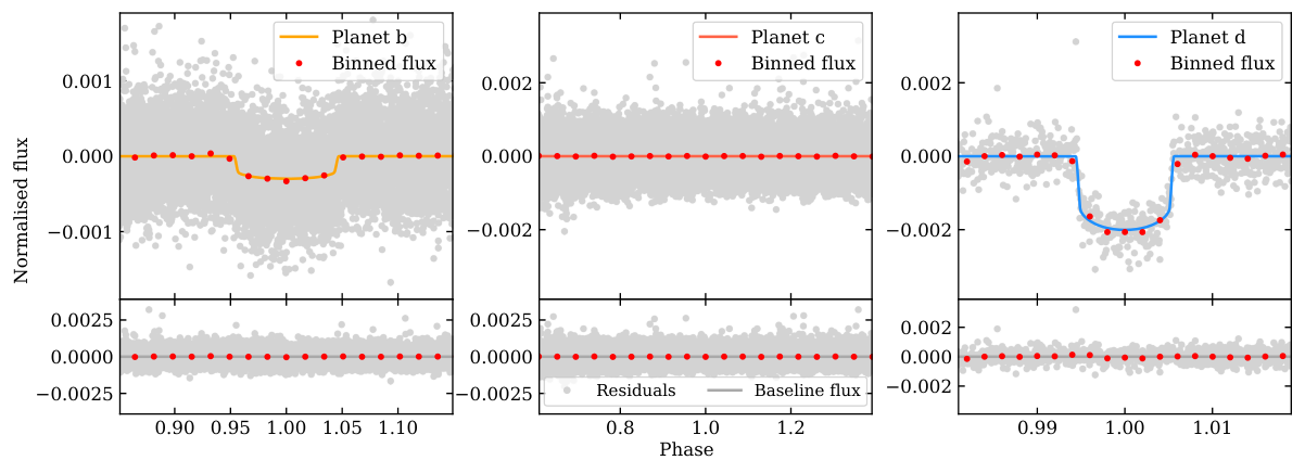
Phase folding the TESS photometry on the RV period reveals no transit (see Fig. 5, bottom plot, middle panel). We also attempted to use Transit Least Squares (Hippke & Heller 2019, TLS,) to recover this planet; it did not return any evidence of a transit at or near the RV period. As this planet is not evident in the TESS data, but is large enough to be detectable (see Section 3.3), we therefore make the assumption that it does not transit. As such, we conclude that this is a further, apparently non-transiting planet, and include it in the final joint fit model (described in Section 3.2) when fitting the RV data.
3.2 Construction of the joint fit model
Using the exoplanet package (Foreman-Mackey et al. 2020), we fit the photometry from TESS, LCOGT, NGTS, and Spitzer and the RVs from HARPS and HIRES simultaneously with Gaussian Processes (GPs) to remove the effects of stellar variability. exoplanet utilises the light curve modelling package Starry (Luger et al. 2019), PyMC3 (Salvatier et al. 2016), and celerite (Foreman-Mackey et al. 2017) to incorporate GPs. While we use a GP kernel included in the exoplanet package for the TESS data, we construct our own GP kernel using PyMC3 for the HARPS and HIRES data. For consistency, all timestamps were converted to the same time system used by TESS, i.e. BJD - 2457000. All prior distributions set on the fit parameters of this model are given in Table 5.
3.2.1 Photometry
The flux is normalised to zero for all of the photometry by dividing the individual light curves by the median of their out-of-transit points and taking away one. To model the planetary transits, we used a limb-darkened transit model following the Kipping 2013b quadratic limb-darkening parameterisation, and Keplerian orbit models. This Keplerian orbit model is parameterised for each planet individually in terms of the stellar radius in solar radii, the stellar mass in solar masses, the orbital period in days, the time of a reference transit , the impact parameter , the eccentricity , and the argument of periastron . While a similar Keplerian orbit model is parameterised for the third planet, is not defined in this case as no transit is seen in the photometric data. We find the eccentricity of all planets to be consistent with 0: when eccentricity is a fit parameter in an earlier run of this model, we find the 95 per cent confidence intervals for the eccentricity of TOI-431 b, c and d to be 0 to 0.28, 0 to 0.22, and 0 to 0.31 respectively. Therefore, we fix and to 0 for all planets in the final joint fit model. These parameters are then input into light curve models created with Starry, together with parameters for the planetary radii , the time series of the data , and the exposure time of the instrument. As we are modelling multiple planets and multiple instruments with different , a separate light curve model is thus created per instrument for the planets that are expected to have a transit event during that data set. In some cases, TOI-431 b and d will have model light curves (e.g. in the TESS and Spitzer observations); in others (e.g. the LCOGT and NGTS observations), only TOI-431 d is expected to be transiting. TOI-431 c is not seen to transit, therefore we do not need to model it in this way. We use values from the TESS pipelines to inform our priors on the epochs, periods, transit depths and radii of the transiting planets.
TESS
Both TOI-431 b and d are transiting in the TESS light curve, so we first create model light curves for each using Starry.
As seen in Fig. 5, the TESS Sector 5 and 6 light curves show some stellar variability. This variability was thus modelled with the SHOTerm GP given in exoplanet 77 7 https://docs.exoplanet.codes/en/stable/user/api/#exoplanet.gp.terms.SHOTerm, which represents a stochastically-driven, damped harmonic oscillator. We set this up using the hyperparameters , , , and . The prior on was set to . Priors on and were set as normal distributions with a mean equal to the log of the variance of the flux and a standard deviation of 0.1. The prior on was also set as a normal distribution but with a mean of 0 and a standard deviation of 0.1 (see Table 5).
We then take the sum of our model light curves and subtract these from the total PDCSAP flux, and this resultant transit-free light curve is the data that the GP is trained on to remove the stellar variability. The GP model can be seen in Fig. 5 (top plot, top panel), and the resultant best fit model in the middle panel. Further to this, phase folds of the TESS data for all planets in the system can also be seen in Fig. 5 (bottom plot), where TOI-431 c has been folded on its period determined from the radial velocity data, and no dip indicative of a transit can be seen.
LCOGT
No further detrending to that outlined in Section 2.1.2 was included for the LCOGT data. Only TOI-431 d is transiting in this data, so we create a model light curve of TOI-431 d using Starry (as outlined above) per LCOGT dataset to produce 2 model light curves overall, as there are 2 transit events - an ingress and an egress - on separate nights. For each dataset, we use a normal prior with the model light curve as the mean and a standard deviation set to the error on the LCOGT data points, and this is then compared to the observed light curve. The best fit model for both the ingress and egress data is shown in Fig. 7 (top 2 panels).
NGTS
No further detrending was needed for the NGTS data after the pipeline reduction outlined in Section 2.1.5, and again, only TOI-431 d is evident in this data. Thus the same simple method used for the LCOGT data above is also applied here, creating a singular model light curve of TOI-431 d for the NGTS data and comparing this to the observed light curve, with a standard deviation set to the error on the NGTS data points. The best fit model for the NGTS data is shown in Fig. 7 (bottom panel).
Spitzer and Pixel Level Decorrelation
For the Spitzer double-transit observation, model light curves are created for both TOI-431 b and d. Spitzer data is given as pixel values on a grid; in this instance, the grid is 3x3 pixels as in figure 1 of Deming et al. 2015. We follow the Pixel Level Decorrelation (PLD) method of Deming et al. 2015 (summarised below) to remove the systematic effect caused by intra-pixel sensitivity variations. Together with pointing jitter, these variations mask the eclipses of exoplanets in the photometry with intensity fluctuations that must be removed. We outline our PLD implementation as follows:
First, the intensity of pixel at each time step , i.e. , is normalised such that the sum of the 9 pixels at one time step is unity, thus removing any astrophysical variations:
| (1) |
PLD makes the simplification that the total flux observed can be expressed as a linear equation:
| (2) |
where is the total fluctuation from all sources. The normalised pixel intensities are multiplied by some coefficient , and summed with the eclipse model , a quadratic function of time which represents the time-dependent “ramp”, and an offset constant . We use the eclipse model set up earlier using exoplanet as , where is the eclipse depth. This allows us to remove the intra-pixel effect, while solving for the eclipse amplitude and temporal baseline effects. Overall, the PLD alone has 14 free parameters that we solve for: 9 pixel coefficients, the depth of eclipse and the eclipse model, 2 time coefficients, and an offset term.
We add an additional fit parameter by introducing a Spitzer “jitter” term. We can estimate a prior for this fit parameter by removing our best fit model from the total raw flux from Spitzer, and calculating the standard deviation of the residual flux, which is approximately 337 ppm.
Our overall model for the Spitzer data is the PLD terms multiplied by the sum of the individual light curve models for each planet, b and d. We use a normal distribution with this model as the mean and a standard deviation set by the jitter parameter, and this is fit to the observed Spitzer flux. This can be seen in Fig. 8.
3.2.2 RVs
We do not include the iSHELL, FEROS, or Minerva-Australis RVs in our joint fit, as they were not found to improve the fit due to large error bars in comparison to the HARPS and HIRES data; however, they are shown to be consistent with the result of our fit (see Fig. 9). We also do not include the archival HARPS data due to a large scatter in cadence and quality in comparison to the purpose-collected HARPS data.
HARPS and HIRES fitting
In this joint fit model, we fit the HARPS and HIRES data using the same method and so they are described here in tandem. We first find predicted values of radial velocity for each planet at each HARPS and HIRES timestamp using exoplanet. We set a wide uniform prior on for each planet, the uniform distributions centred upon values found when fitting the RV data with simple Keplerian models for all of the planets in DACE. We fit separate “offset” terms for HARPS and HIRES to model the systematic radial velocity, giving this a normal prior with a mean value predicted in DACE. We also fit separate “jitter” terms, setting wide normal priors on these, the means of which are set to double the log of the minimum error on the HARPS and HIRES data respectively.
The RV data also shows significant stellar variability due to stellar rotation, and so we model this variability using another GP (see Fig. 9, top panel of top plot). This activity can be modelled as a Quasi-Periodic signal as starspots moving across the surface of the star evolve in time and are modulated by stellar rotation. In this case, we create our own Quasi-Periodic kernel using PyMC3, as no such kernel is available in exoplanet. PyMC3 provides a range of simple kernels88
8
https://docs.pymc.io/api/gp/cov.html which are easy to combine. We use their Periodic:
| (3) |
and ExpQuad (squared exponential):
| (4) |
kernels. The hyperparameters are (the amplitude of the GP), (the recurrence timescale, equivalent to the of the star), (the smoothing parameter), and (the timescale for growth and decay of active regions) (Rasmussen & Williams 2006; Haywood et al. 2014; Grunblatt et al. 2015, see e.g.).
We multiply these kernels together to create our final Quasi-Periodic kernel:
| (5) |
We use the same GP to fit the HARPS and HIRES data together using the same hyperparameters. We use a normal distribution with a mean equal to the rotation period of the star found by WASP-South (see Section 2.5 and Table 2) to set a wide prior on .
To bring everything together, we add the predicted radial velocities together with the offsets, and subtract these from their respective observed radial velocity values. This is then used as the prior on the GP, which is also given a noise term that is equal to an addition of the jitters with the squared error on the RV data.
3.3 Fit results
We first use exoplanet to maximise the log probability of the PyMC3 model. We then use the fit parameter values this obtains as the starting point of the PyMC3 sampler, which draws samples from the posterior using a variant of Hamiltonian Monte Carlo, the No-U-Turn Sampler (NUTS). By examining the chains from earlier test runs of the model, we allow for 1000 burn-in samples which are discarded, and 5000 steps with 15 chains.
We present our best fit parameters for the TOI-431 system from our joint fit in Table 3. TOI-431 b is a super-Earth with a mass of M⊕and a radius of 1.28 0.04 R⊕, and from this we can infer a bulk density of g cm-3. This puts TOI-431 b below the radius gap, and it is likely a stripped core with no gaseous envelope. A period of 0.49 days puts TOI-431 b in the rare Ultra-Short Period (USP) planet category (defined simply as planets with day); examples of systems which have USP planets include Kepler-78 (Winn et al. 2018), WASP-47 (Becker et al. 2015), and 55 Cancri (Dawson & Fabrycky 2010). TOI-431 c has a minimum mass of M⊕, but the lack of transits does not allow us to fit a radius. We can use the mass-radius relation via forecaster (Chen & Kipping 2017) to estimate a radius of R⊕, which would place this planet as another super-Earth. TOI-431 d is a sub-Neptune with a mass of M⊕and a radius of R⊕, implying a bulk density of g cm-3. This lower density implies that TOI-431 d probably has a gaseous envelope. We further analyse these planets in the following section.
| Parameter | TOI-431 b | TOI-431 c | TOI-431 d |
|---|---|---|---|
| Period (days) | 12.46103 0.00002 | ||
| Semi-major axis (AU) | 0.052 0.001 | 0.098 0.002 | |
| Ephemeris (BJD-2457000) | |||
| Radius (R⊕) | 1.28 0.04 | - | |
| Impact parameter | - | ||
| Inclination (degrees) | |||
| Eccentricity | 0 (fixed) | 0 (fixed) | 0 (fixed) |
| The argument of periastron | 0 (fixed) | 0 (fixed) | 0 (fixed) |
| Radial velocity semi-amplitude () | 2.88 0.30 | ||
| Mass (M⊕) | () | ||
| Bulk density (g cm-3) | - | ||
| Equilibrium temperature (K) | 633 14 |
4 Discussion
The architecture of this system is unusual in that the middle planet, TOI-431 c, is non-transiting, while the inner and outer planets are both seen to transit. Examples of this can be seen in Kepler-20 (Buchhave et al. 2016), a 6-planet system where the fifth planet out from the star does not transit, but the sixth does, and HD 3167 (Vanderburg et al. 2016; Gandolfi et al. 2017; Christiansen et al. 2017), a 3-planet system where the middle planet does not transit as is the case with TOI-431. Using the impact parameter from Table 3, we calculate inclinations for TOI-431 b and d of and , respectively (Table 3). We can calculate a limit on the inclination for TOI-431 c assuming , which results in an inclination that must be in order for TOI-431 c to be non-transiting.
The TOI-431 system is a good target system for studying planetary evolution. TOI-431 b and d reside either side of the radius-period valley described in Fulton et al. 2017; Fulton & Petigura 2018; Van Eylen et al. 2018 (see Fig. 10), providing a useful test-bed for the theorised mechanisms behind it. X-ray and EUV-driven photoevaporation is one of the two main proposed mechanisms (Owen & Wu 2017), and we investigated its effect both now and in the past in the TOI-431 system. As no direct X-ray observations of the system exist, we had to make use of empirical formulae for relating the ratio of the X-ray and bolometric luminosities to age (Jackson et al. 2012) and Rossby number (related to , Wright et al. 2011; Wright et al. 2018). We extrapolate to the EUV using the relations of King et al. 2018. Under the assumption of energy-limited escape (Watson et al. 1981; Erkaev et al. 2007), we estimate a current mass loss rate for TOI-431 d between and g s-1. The same assumptions yield a current rate of to g s-1 for TOI-431 b, but since that planet is unlikely to retain much, if any, atmosphere, the likely true rate is much lower.
Integrating the Jackson et al. 2012 relations across the lifetime of the star, and again assuming energy-limited escape, lifetime-to-date mass loss estimates of 44 per cent and 1.0 per cent for TOI-431 b and d respectively are found. Adding 2 per cent extra mass and doubling the radius to account for a primordial envelope around TOI-431 b raises the lifetime loss to 94 per cent. Again, the true value will be lower as XUV photoevaporation will not affect the rocky core, but rather the estimates calculated here demonstrate TOI-431 b would easily have lost a typical envelope with a mass fraction of a few per cent. The value for TOI-431 d is consistent with the density of the planet, which suggests it retains a substantial envelope.
In order to characterize the composition of TOI-431 b and TOI-431 d, we model the interior considering a pure-iron core, a silicate mantle, a pure-water layer, and a H-He atmosphere. The models follow the basic structure model of Dorn et al. 2017, with the equation of state (EOS) of the iron core taken from Hakim et al. 2018, the EOS of the silicate-mantle from Connolly 2009, and SCVH (Saumon et al. 1995) for the H-He envelope assuming protosolar composition. For water we use the QEOS of Vazan et al. 2013 for low pressures and the one of Seager et al. 2007 for pressures above 44.3 GPa.
Fig. 11 shows M-R curves tracing compositions of pure-iron, Earth-like, pure-water and a planet with 95 per cent water and 5 per cent H-He atmosphere subjected to a stellar radiation of = 50 (comparable to the case of the TOI-431 planets), and exoplanets with accurate and reliable mass and radius determinations. It should be noted that the position of the water line in the diagram is very sensitive to used EOS (Haldemann et al. 2020, e.g.). Fig. 11 shows two water lines using QEOS and EOS from Sotin et al. 2007. As shown in Fig. 11, TOI-431 b is one of the many super-Earths following the Earth-like composition line. This suggests that it is mostly made of refractory materials. TOI-431 d, instead, sits above the two the pure-water curves and below the 5 per cent curve, implying that the H-He mass fraction is unlikely to exceed a few per cent. Its density is lower than most of the observed sub-Neptunes. There are three planets in the catalogue presented in Otegi et al. 2020b with masses below 10 M⊕ and radii above 3 R⊕ (Kepler-11 d,e and Kepler-36 c), and all of their masses have been determined with TTVs. As shown in Otegi et al. 2020a, reducing the uncertainties in this M-R regime would lead to significant improvements on the determination of the volatile envelope mass. As TOI-431 is in the ESPRESSO GTO target list, more observations will help to further constrain the internal structure of TOI-431 d.
We then quantify the degeneracy between the different interior parameters and produce posterior probability distributions using a generalised Bayesian inference analysis with a Nested Sampling scheme (Buchner 2014, e.g.). The interior parameters that are inferred include the masses of the pure-iron core, silicate mantle, water layer and H-He atmospheres. For the analysis, we use the stellar Fe/Si and Mg/Si ratios as a proxy for the planet. Table 4 lists the inferred mass fractions of the core, mantle, water-layer and H-He atmosphere from the interior models. It should be noted, however, that our estimates have rather large uncertainties. Indeed, in this regime of the M-R relation there is a large degeneracy, and therefore the mass ratio between the planetary layers is not well-constrained. Nevertheless, we find that TOI-431 b has a negligible H-He envelope of 1.2x.
The larger companion TOI-431 d is expected to have a significant volatile layer of H-He and/or water of about 3.6 or 33 per cent of its total mass, respectively. The nature of the volatile layer is degenerate.
| Interior Structure: | TOI-431 b | TOI-431 d |
|---|---|---|
| - |
Considering the future observation prospects of this system, for TOI-431 d we calculate a transmission spectroscopy metric (Kempton et al. 2018, TSM;) of , after propagating the uncertainties on all system parameters. The relatively large uncertainty is dominated by the uncertainty on the planet’s mass; nonetheless, this TSM value indicates that TOI-431 d is likely among the best transmission spectroscopy targets known among small, cool exoplanets (Guo et al. 2020, , K; see Table 11 of).
5 Conclusion
We have presented here the discovery of three new planets from the TESS mission in the TOI-431 system. Our analysis is based upon 2-min cadence TESS observations from 2 sectors, ground-based follow-up from LCOGT and NGTS, and space-based follow-up from Spitzer. The photometric data was modelled jointly with RV data from the HARPS spectrograph, and further RVs from iSHELL, FEROS, and Minerva-Australis are included in our analysis. We find evidence to suggest that the host star is rotating with a period of 30.5 days, and account for this in our joint-fit model. Nearby contaminating stellar companions are ruled out by multiple sources of high resolution imaging.
TOI-431 b is a super-Earth characterised by both photometry and RVs, with an ultra-short period of 0.49 days. It likely has a negligible envelope due to substantial atmosphere evolution via photoevaporation, and an Earth-like composition.
TOI-431 c is found in the HARPS RV data and is not seen to transit. It has a period of 4.84 days and a minimum mass similar to the mass of TOI-431 b; extrapolating this minimum mass to a radius via the MR relation places it as a likely second super-Earth.
TOI-431 d is a sub-Neptune with a period of 12.46 days, characterised by both photometry and RVs. It has likely retained a substantial H-He envelope of about 4 per cent of its total mass. Additionally, TOI-431 b and d contribute to the TESS Level-1 mission requirement.
This system is a candidate for further study of planetary evolution, with TOI-431 b and d either side of the radius valley. The system is bright, making it amenable to follow-up observations. TOI-431 b, in particular, would potentially be an interesting target for phase-curve observations with JWST.
Acknowledgements
This paper includes data collected by the TESS mission. Funding for the TESS mission is provided by the NASA Explorer Program. Resources supporting this work were provided by the NASA High-End Computing (HEC) Program through the NASA Advanced Supercomputing (NAS) Division at Ames Research Center for the production of the SPOC data products.
We acknowledge the use of public TESS Alert data from pipelines at the TESS Science Office and at the TESS Science Processing Operations Center.
This study is based on observations collected at the European Southern Observatory under ESO programme 1102.C-0249 (PI: Armstrong). Additionally the archival HARPS data dating from 2004 to 2015 were obtained under the following programmes: 072.C-0488 (PI: Mayor); 183.C-0972 (PI: Udry); 085.C-0019 (PI: Lo Curto); 087.C-0831 (PI: Lo Curto); and 094.C-0428 (PI: Brahm).
This work was supported by grants to P.P. from NASA (award 18-2XRP18_2-0113), the National Science Foundation (Astronomy and Astrophysics grant 1716202), the Mount Cuba Astronomical Foundation, and George Mason University start-up funds.The NASA Infrared Telescope Facility is operated by the University of Hawaii under contract NNH14CK55B with NASA.
This paper is in part based on data collected under the NGTS project at the ESO La Silla Paranal Observatory. The NGTS facility is operated by the consortium institutes with support from the UK Science and Technology Facilities Council (STFC) projects ST/M001962/1 and ST/S002642/1.
This work makes use of observations from the LCOGT network.
Minerva-Australis is supported by Australian Research Council LIEF Grant LE160100001, Discovery Grant DP180100972, Mount Cuba Astronomical Foundation, and institutional partners University of Southern Queensland, UNSW Sydney, MIT, Nanjing University, George Mason University, University of Louisville, University of California Riverside, University of Florida, and The University of Texas at Austin.
We respectfully acknowledge the traditional custodians of all lands throughout Australia, and recognise their continued cultural and spiritual connection to the land, waterways, cosmos, and community. We pay our deepest respects to all Elders, ancestors and descendants of the Giabal, Jarowair, and Kambuwal nations, upon whose lands the Minerva-Australis facility at Mt Kent is situated.
This work is based in part on observations made with the Spitzer Space Telescope, which was operated by the Jet Propulsion Laboratory, California Institute of Technology under a contract with NASA. Support for this work was provided by NASA through an award issued by JPL/Caltech.
Based on observations obtained at the international Gemini Observatory, a program of NSF’s NOIRLab acquired through the Gemini Observatory Archive at NSF’s NOIRLab, which is managed by the Association of Universities for Research in Astronomy (AURA) under a cooperative agreement with the National Science Foundation on behalf of the Gemini Observatory partnership: the National Science Foundation (United States), National Research Council (Canada), Agencia Nacional de Investigación y Desarrollo (Chile), Ministerio de Ciencia, Tecnología e Innovación (Argentina), Ministério da Ciência, Tecnologia, Inovações e Comunicações (Brazil), and Korea Astronomy and Space Science Institute (Republic of Korea). Data collected under program GN-2019A-LP-101.
This work was enabled by observations made from the Gemini North telescope, located within the Maunakea Science Reserve and adjacent to the summit of Maunakea. We are grateful for the privilege of observing the Universe from a place that is unique in both its astronomical quality and its cultural significance.
This work is based in part on observations obtained at the Southern Astrophysical Research (SOAR) telescope, which is a joint project of the Ministério da Ciência, Tecnologia e Inovações (MCTI/LNA) do Brasil, the US National Science Foundation’s NOIRLab, the University of North Carolina at Chapel Hill (UNC), and Michigan State University (MSU).
This research made use of exoplanet (Foreman-Mackey et al. 2020) and its dependencies (Agol et al. 2019; Astropy Collaboration et al. 2013; Astropy Collaboration et al. 2018; Foreman-Mackey et al. 2020; Kipping 2013a; Luger et al. 2019; Salvatier et al. 2016; Theano Development Team 2016).
This publication makes use of The Data & Analysis Center for Exoplanets (DACE), which is a facility based at the University of Geneva (CH) dedicated to extrasolar planets data visualisation, exchange and analysis. DACE is a platform of the Swiss National Centre of Competence in Research (NCCR) PlanetS, federating the Swiss expertise in Exoplanet research. The DACE platform is available at https://dace.unige.ch.
This work has made use of data from the European Space Agency (ESA) mission Gaia (https://www.cosmos.esa.int/gaia), processed by the Gaia Data Processing and Analysis Consortium (DPAC, https://www.cosmos.esa.int/web/gaia/dpac/consortium). Funding for the DPAC has been provided by national institutions, in particular the institutions participating in the Gaia Multilateral Agreement.
AO is supported by an STFC studentship. DJA acknowledges support from the STFC via an Ernest Rutherford Fellowship (ST/R00384X/1). RB acknowledges support from FONDECYT Post-doctoral Fellowship Project 3180246, and from the Millennium Institute of Astrophysics (MAS). IJMC acknowledges support from the NSF through grant AST-1824644. AJ acknowledges support from FONDECYT project 1210718, and from ANID – Millennium Science Initiative – ICN12_009. MNG. acknowledges support from MIT’s Kavli Institute as a Juan Carlos Torres Fellow. JSJ acknowledges support by FONDECYT grant 1201371 and partial support from CONICYT project Basal AFB-170002. We acknowledge support by FCT - Fundação para a Ciência e a Tecnologia through national funds and by FEDER through COMPETE2020 - Programa Operacional Competitividade e Internacionalização by these grants: UID/FIS/04434/2019; UIDB/04434/2020; UIDP/04434/2020; PTDC/FIS-AST/32113/2017 & POCI-01-0145-FEDER-032113; PTDC/FIS-AST/28953/2017 & POCI-01-0145-FEDER-028953. VA, EDM and SCCB acknowledge the support from FCT through Investigador FCT contracts IF/00650/2015/CP1273/CT0001, IF/00849/2015/CP1273/CT0003, and IF/01312/2014/CP1215/CT0004 respectively. ODSD is supported in the form of work contract (DL 57/2016/CP1364/CT0004) funded by FCT. CD acknowledges the SNSF Ambizione Grant 174028. SH acknowledge support by the fellowships PD/BD/128119/2016 funded by FCT (Portugal). JKT acknowledges that support for this work was provided by NASA through Hubble Fellowship grant HST-HF2-51399.001 awarded by the Space Telescope Science Institute, which is operated by the Association of Universities for Research in Astronomy, Inc., for NASA, under contract NAS5-26555. DD acknowledges support through the TESS Guest Investigator Program Grant 80NSSC19K1727. JLB and DB have been supported by the Spanish State Research Agency (AEI) Project No. MDM-2017-0737 Unidad de Excelencia “María de Maeztu”- Centro de Astrobiología (CSIC/INTA). SH acknowledges CNES funding through the grant 837319. PJW acknowledges support from STFC through consolidated grants ST/P000495/1 and ST/T000406/1. L.M.W. is supported by the Beatrice Watson Parrent Fellowship and NASA ADAP Grant 80NSSC19K0597.
Data Availability
The TESS data are available from the Mikulski Archive for Space Telescopes (MAST), at https://heasarc.gsfc.nasa.gov/docs/tess/data-access.html. The other photometry from the LCOGT, NGTS, and Spitzer as well as all of the RV data, are available for public download from the ExoFOP-TESS archive at https://exofop.ipac.caltech.edu/tess/target.php?id=31374837. This data is labelled “Osborn+ 2021” in their descriptions. The high-resolution imaging data is also available from the ExoFOP TESS archive. The model code underlying this article will be shared on reasonable request to the corresponding author.
References
- Addison et al. (2019a) Addison B., et al., 2019a, PASP, 131, 115003
- Addison et al. (2019b) Addison B., et al., 2019b, PASP, 131, 115003
- Addison et al. (2020) Addison B. C., et al., 2020, arXiv e-prints, p. arXiv:2001.07345
- Adibekyan et al. (2012) Adibekyan V. Z., Sousa S. G., Santos N. C., Delgado Mena E., González Hernández J. I., Israelian G., Mayor M., Khachatryan G., 2012, A&A, 545, A32
- Adibekyan et al. (2015) Adibekyan V., et al., 2015, A&A, 583, A94
- Agol et al. (2019) Agol E., Luger R., Foreman-Mackey D., 2019, arXiv e-prints
- Armstrong et al. (2020) Armstrong D. J., et al., 2020, Nature, 583, 39
- Astropy Collaboration et al. (2013) Astropy Collaboration et al., 2013, aap, 558, A33
- Astropy Collaboration et al. (2018) Astropy Collaboration et al., 2018, aj, 156, 123
- Astudillo-Defru et al. (2020) Astudillo-Defru N., et al., 2020, A&A, 636, A58
- Bailer-Jones et al. (2021) Bailer-Jones C. A. L., Rybizki J., Fouesneau M., Demleitner M., Andrae R., 2021, AJ, 161, 147
- Barbary (2016) Barbary K., 2016, Journal of Open Source Software, 1, 58
- Barnes et al. (2012) Barnes S. I., Gibson S., Nield K., Cochrane D., 2012, in Ground-based and Airborne Instrumentation for Astronomy IV. p. 844688, doi:10.1117/12.926527
- Beaugé & Nesvorný (2013) Beaugé C., Nesvorný D., 2013, ApJ, 763, 12
- Becker et al. (2015) Becker J. C., Vanderburg A., Adams F. C., Rappaport S. A., Schwengeler H. M., 2015, ApJ, 812, L18
- Bertin & Arnouts (1996) Bertin E., Arnouts S., 1996, A&AS, 117, 393
- Bhatti et al. (2020) Bhatti W., Bouma L., Joshua John Price-Whelan A., 2020, waqasbhatti/astrobase: astrobase v0.5.0, doi:10.5281/zenodo.3723832, https://doi.org/10.5281/zenodo.3723832
- Borucki et al. (2010) Borucki W. J., et al., 2010, Science, 327, 977
- Brahm et al. (2017) Brahm R., Jordán A., Espinoza N., 2017, PASP, 129, 034002
- Brahm et al. (2019) Brahm R., et al., 2019, AJ, 158, 45
- Brown et al. (2013) Brown T. M., et al., 2013, PASP, 125, 1031
- Bruntt et al. (2010) Bruntt H., et al., 2010, MNRAS, 405, 1907
- Bryant et al. (2020) Bryant E. M., et al., 2020, arXiv e-prints, p. arXiv:2004.07589
- Buchhave et al. (2016) Buchhave L. A., et al., 2016, AJ, 152, 160
- Buchner (2014) Buchner J., 2014, arXiv e-prints, p. arXiv:1407.5459
- Cale et al. (2019) Cale B., et al., 2019, AJ, 158, 170
- Chabrier (2001) Chabrier G., 2001, ApJ, 554, 1274
- Chen & Kipping (2017) Chen J., Kipping D., 2017, ApJ, 834, 17
- Christiansen et al. (2017) Christiansen J. L., et al., 2017, AJ, 154, 122
- Ciardi et al. (2015) Ciardi D. R., Beichman C. A., Horch E. P., Howell S. B., 2015, ApJ, 805, 16
- Cloutier & Menou (2020) Cloutier R., Menou K., 2020, AJ, 159, 211
- Cloutier et al. (2019) Cloutier R., et al., 2019, A&A, 629, A111
- Cloutier et al. (2020a) Cloutier R., et al., 2020a, AJ, 160, 3
- Cloutier et al. (2020b) Cloutier R., et al., 2020b, AJ, 160, 22
- Collins et al. (2017) Collins K. A., Kielkopf J. F., Stassun K. G., Hessman F. V., 2017, AJ, 153, 77
- Connolly (2009) Connolly J. A. D., 2009, Geochemistry, Geophysics, Geosystems, 10, Q10014
- Crossfield et al. (2018) Crossfield I., et al., 2018, Spitzer Transits of New TESS Planets, Spitzer Proposal
- Dawson & Fabrycky (2010) Dawson R. I., Fabrycky D. C., 2010, ApJ, 722, 937
- Delgado Mena et al. (2017) Delgado Mena E., Tsantaki M., Adibekyan V. Z., Sousa S. G., Santos N. C., González Hernández J. I., Israelian G., 2017, A&A, 606, A94
- Delgado Mena et al. (2019) Delgado Mena E., et al., 2019, A&A, 624, A78
- Deming et al. (2015) Deming D., et al., 2015, ApJ, 805, 132
- Díaz et al. (2020) Díaz M. R., et al., 2020, MNRAS, 493, 973
- Dorn et al. (2017) Dorn C., Venturini J., Khan A., Heng K., Alibert Y., Helled R., Rivoldini A., Benz W., 2017, A&A, 597, A37
- Doyle et al. (2014) Doyle A. P., Davies G. R., Smalley B., Chaplin W. J., Elsworth Y., 2014, MNRAS, 444, 3592
- Dragomir et al. (2019) Dragomir D., et al., 2019, ApJ, 875, L7
- Dumusque et al. (2019) Dumusque X., et al., 2019, A&A, 627, A43
- Erkaev et al. (2007) Erkaev N. V., Kulikov Y. N., Lammer H., Selsis F., Langmayr D., Jaritz G. F., Biernat H. K., 2007, A&A, 472, 329
- Fazio et al. (2004) Fazio G. G., et al., 2004, ApJS, 154, 10
- Foreman-Mackey et al. (2017) Foreman-Mackey D., Agol E., Ambikasaran S., Angus R., 2017, celerite: Scalable 1D Gaussian Processes in C++, Python, and Julia (ascl:1709.008)
- Foreman-Mackey et al. (2020) Foreman-Mackey D., Czekala I., Luger R., Agol E., Barentsen G., Barclay T., 2020, exoplanet-dev/exoplanet v0.2.6, doi:10.5281/zenodo.1998447, https://doi.org/10.5281/zenodo.1998447
- Fressin et al. (2013) Fressin F., et al., 2013, ApJ, 766, 81
- Fulton & Petigura (2018) Fulton B. J., Petigura E. A., 2018, AJ, 156, 264
- Fulton et al. (2017) Fulton B. J., et al., 2017, AJ, 154, 109
- Furlan et al. (2017) Furlan E., et al., 2017, AJ, 153, 71
- Gaia Collaboration et al. (2016) Gaia Collaboration et al., 2016, A&A, 595, A2
- Gaia Collaboration et al. (2018) Gaia Collaboration et al., 2018, A&A, 616, A1
- Gaia Collaboration et al. (2021) Gaia Collaboration et al., 2021, A&A, 649, A1
- Gandolfi et al. (2017) Gandolfi D., et al., 2017, AJ, 154, 123
- Gandolfi et al. (2018) Gandolfi D., et al., 2018, A&A, 619, L10
- Girardi et al. (2012) Girardi L., et al., 2012, Astrophysics and Space Science Proceedings, 26, 165
- Grunblatt et al. (2015) Grunblatt S. K., Howard A. W., Haywood R. D., 2015, ApJ, 808, 127
- Günther et al. (2019) Günther M. N., et al., 2019, Nature Astronomy, 3, 1099
- Guo et al. (2020) Guo X., et al., 2020, AJ, 159, 239
- Gustafsson et al. (2008) Gustafsson B., Edvardsson B., Eriksson K., Jørgensen U. G., Nordlund Å., Plez B., 2008, A&A, 486, 951
- Hakim et al. (2018) Hakim K., Rivoldini A., Van Hoolst T., Cottenier S., Jaeken J., Chust T., Steinle-Neumann G., 2018, Icarus, 313, 61
- Haldemann et al. (2020) Haldemann J., Alibert Y., Mordasini C., Benz W., 2020, arXiv e-prints, p. arXiv:2009.10098
- Haywood et al. (2014) Haywood R. D., et al., 2014, MNRAS, 443, 2517
- Helled et al. (2016) Helled R., Lozovsky M., Zucker S., 2016, MNRAS, 455, L96
- Hippke & Heller (2019) Hippke M., Heller R., 2019, TLS: Transit Least Squares (ascl:1910.007)
- Hirano et al. (2018) Hirano T., et al., 2018, AJ, 155, 127
- Hodapp et al. (2003) Hodapp K. W., et al., 2003, PASP, 115, 1388
- Howard et al. (2010) Howard A. W., et al., 2010, ApJ, 721, 1467
- Howell et al. (2011) Howell S. B., Everett M. E., Sherry W., Horch E., Ciardi D. R., 2011, AJ, 142, 19
- Huang et al. (2018) Huang C. X., et al., 2018, ApJ, 868, L39
- Huang et al. (2019) Huang X., Burt J., Vanderburg A., Gunther M., Shporer A., Dittmann J., Winn J., 2019, in American Astronomical Society Meeting Abstracts #233. p. 209.08
- Isaacson & Fischer (2010) Isaacson H., Fischer D., 2010, ApJ, 725, 875
- Jackson et al. (2012) Jackson A. P., Davis T. A., Wheatley P. J., 2012, MNRAS, 422, 2024
- Jenkins et al. (2016) Jenkins J. M., et al., 2016, The TESS science processing operations center. p. 99133E, doi:10.1117/12.2233418
- Jensen (2013) Jensen E., 2013, Tapir: A web interface for transit/eclipse observability (ascl:1306.007)
- Jordán et al. (2020) Jordán A., Brahm R., Espinoza N., Henning T., Jones M. I., Kossakowski D., Sarkis P., Trifonov T., 2020, AJ, 159, 145
- Kaufer & Pasquini (1998) Kaufer A., Pasquini L., 1998, FEROS: the new fiber-linked echelle spectrograph for the ESO 1.52-m telescope. pp 844–854, doi:10.1117/12.316798
- Kaufer et al. (1999) Kaufer A., Stahl O., Tubbesing S., Nørregaard P., Avila G., Francois P., Pasquini L., Pizzella A., 1999, The Messenger, 95, 8
- Kempton et al. (2018) Kempton E. M. R., et al., 2018, PASP, 130, 114401
- King et al. (2018) King G. W., et al., 2018, MNRAS, 478, 1193
- Kipping (2013a) Kipping D. M., 2013a, mnras, 435, 2152
- Kipping (2013b) Kipping D. M., 2013b, MNRAS, 435, 2152
- Kurucz (1993) Kurucz R. L., 1993, SYNTHE spectrum synthesis programs and line data
- Li et al. (2019) Li J., Tenenbaum P., Twicken J. D., Burke C. J., Jenkins J. M., Quintana E. V., Rowe J. F., Seader S. E., 2019, PASP, 131, 024506
- Lillo-Box et al. (2014) Lillo-Box J., Barrado D., Bouy H., 2014, A&A, 566, A103
- Luger et al. (2019) Luger R., Agol E., Foreman-Mackey D., Fleming D. P., Lustig-Yaeger J., Deitrick R., 2019, aj, 157, 64
- Lundkvist et al. (2016) Lundkvist M. S., et al., 2016, Nature Communications, 7, 11201
- Luque et al. (2019) Luque R., et al., 2019, A&A, 628, A39
- Mamajek & Hillenbrand (2008) Mamajek E. E., Hillenbrand L. A., 2008, ApJ, 687, 1264
- Maxted et al. (2011) Maxted P. F. L., et al., 2011, PASP, 123, 547
- Mazeh et al. (2016) Mazeh T., Holczer T., Faigler S., 2016, A&A, 589, A75
- McCormac et al. (2013) McCormac J., Pollacco D., Skillen I., Faedi F., Todd I., Watson C. A., 2013, PASP, 125, 548
- McCully et al. (2018) McCully C., Volgenau N. H., Harbeck D.-R., Lister T. A., Saunders E. S., Turner M. L., Siiverd R. J., Bowman M., 2018, in Proc. SPIE. p. 107070K (arXiv:1811.04163), doi:10.1117/12.2314340
- Mortier et al. (2014) Mortier A., Sousa S. G., Adibekyan V. Z., Brand ão I. M., Santos N. C., 2014, A&A, 572, A95
- Nielsen et al. (2020) Nielsen L. D., et al., 2020, MNRAS, 492, 5399
- Otegi et al. (2020a) Otegi J. F., Dorn C., Helled R., Bouchy F., Haldemann J., Alibert Y., 2020a, arXiv e-prints, p. arXiv:2006.12353
- Otegi et al. (2020b) Otegi J. F., Bouchy F., Helled R., 2020b, A&A, 634, A43
- Owen & Lai (2018) Owen J. E., Lai D., 2018, MNRAS, 479, 5012
- Owen & Wu (2017) Owen J. E., Wu Y., 2017, ApJ, 847, 29
- Pepe et al. (2002) Pepe F., et al., 2002, The Messenger, 110, 9
- Persson et al. (2018) Persson C. M., et al., 2018, A&A, 618, A33
- Petigura et al. (2013) Petigura E. A., Howard A. W., Marcy G. W., 2013, Proceedings of the National Academy of Science, 110, 19273
- Piskunov & Valenti (2017) Piskunov N., Valenti J. A., 2017, A&A, 597, A16
- Piskunov et al. (1995) Piskunov N. E., Kupka F., Ryabchikova T. A., Weiss W. W., Jeffery C. S., 1995, A&AS, 112, 525
- Pollacco et al. (2006) Pollacco D. L., et al., 2006, PASP, 118, 1407
- Rasmussen & Williams (2006) Rasmussen C. E., Williams C. K. I., 2006, Gaussian Processes for Machine Learning
- Rayner et al. (2016a) Rayner J., et al., 2016a, iSHELL: a construction, assembly and testing. p. 990884, doi:10.1117/12.2232064
- Rayner et al. (2016b) Rayner J., et al., 2016b, in Proc. SPIE. p. 990884, doi:10.1117/12.2232064
- Ricker et al. (2015) Ricker G. R., et al., 2015, Journal of Astronomical Telescopes, Instruments, and Systems, 1, 014003
- Salvatier et al. (2016) Salvatier J., Wiecki T. V., Fonnesbeck C., 2016, PeerJ Computer Science, 2, e55
- Santos et al. (2013) Santos N. C., et al., 2013, A&A, 556, A150
- Saumon et al. (1995) Saumon D., Chabrier G., van Horn H. M., 1995, ApJS, 99, 713
- Seager et al. (2007) Seager S., Kuchner M., Hier-Majumder C. A., Militzer B., 2007, ApJ, 669, 1279
- Skrutskie et al. (2006) Skrutskie M. F., et al., 2006, AJ, 131, 1163
- Smith et al. (2012) Smith J. C., et al., 2012, PASP, 124, 1000
- Smith et al. (2020) Smith A. M. S., et al., 2020, arXiv e-prints, p. arXiv:2002.05591
- Sneden (1973) Sneden C. A., 1973, PhD thesis, THE UNIVERSITY OF TEXAS AT AUSTIN.
- Sotin et al. (2007) Sotin C., Grasset O., Mocquet A., 2007, Icarus, 191, 337
- Sousa (2014) Sousa S. G., 2014, [arXiv:1407.5817],
- Sousa et al. (2015) Sousa S. G., Santos N. C., Adibekyan V., Delgado-Mena E., Israelian G., 2015, A&A, 577, A67
- Stassun & Torres (2016) Stassun K. G., Torres G., 2016, AJ, 152, 180
- Stassun & Torres (2021) Stassun K. G., Torres G., 2021, ApJ, 907, L33
- Stassun et al. (2017) Stassun K. G., Collins K. A., Gaudi B. S., 2017, AJ, 153, 136
- Stassun et al. (2018) Stassun K. G., Corsaro E., Pepper J. A., Gaudi B. S., 2018, AJ, 155, 22
- Stassun et al. (2019) Stassun K. G., et al., 2019, AJ, 158, 138
- Stumpe et al. (2012) Stumpe M. C., et al., 2012, PASP, 124, 985
- Stumpe et al. (2014) Stumpe M. C., Smith J. C., Catanzarite J. H., Van Cleve J. E., Jenkins J. M., Twicken J. D., Girouard F. R., 2014, PASP, 126, 100
- Szabó & Kiss (2011) Szabó G. M., Kiss L. L., 2011, ApJ, 727, L44
- Theano Development Team (2016) Theano Development Team 2016, arXiv e-prints, abs/1605.02688
- Tokovinin (2018) Tokovinin A., 2018, PASP, 130, 035002
- Torres et al. (2010) Torres G., Andersen J., Giménez A., 2010, A&ARv, 18, 67
- Twicken et al. (2010) Twicken J. D., Chandrasekaran H., Jenkins J. M., Gunter J. P., Girouard F., Klaus T. C., 2010, in Proc. SPIE. p. 77401U, doi:10.1117/12.856798
- Twicken et al. (2018) Twicken J. D., et al., 2018, PASP, 130, 064502
- Valenti & Piskunov (1996) Valenti J. A., Piskunov N., 1996, A&AS, 118, 595
- Van Eylen et al. (2018) Van Eylen V., Agentoft C., Lundkvist M. S., Kjeldsen H., Owen J. E., Fulton B. J., Petigura E., Snellen I., 2018, MNRAS, 479, 4786
- Vanderburg et al. (2016) Vanderburg A., et al., 2016, ApJ, 829, L9
- Vazan et al. (2013) Vazan A., Kovetz A., Podolak M., Helled R., 2013, MNRAS, 434, 3283
- Vogt et al. (1994) Vogt S. S., et al., 1994, in Crawford D. L., Craine E. R., eds, Society of Photo-Optical Instrumentation Engineers (SPIE) Conference Series Vol. 2198, Instrumentation in Astronomy VIII. p. 362, doi:10.1117/12.176725
- Watson et al. (1981) Watson A. J., Donahue T. M., Walker J. C. G., 1981, Icarus, 48, 150
- Wheatley et al. (2018) Wheatley P. J., et al., 2018, MNRAS, 475, 4476
- Winn et al. (2018) Winn J. N., Sanchis-Ojeda R., Rappaport S., 2018, New Astron. Rev., 83, 37
- Wright et al. (2011) Wright N. J., Drake J. J., Mamajek E. E., Henry G. W., 2011, ApJ, 743, 48
- Wright et al. (2018) Wright N. J., Newton E. R., Williams P. K. G., Drake J. J., Yadav R. K., 2018, MNRAS, 479, 2351
- Yee et al. (2017) Yee S. W., Petigura E. A., von Braun K., 2017, ApJ, 836, 77
- Ziegler et al. (2020) Ziegler C., Tokovinin A., Briceño C., Mang J., Law N., Mann A. W., 2020, AJ, 159, 19
Appendix A Further Joint Fit Parameters
Parameter
Prior Distribution
Fit Value
Planets
Period [b] (days)
Period [c] (days)
Period [d] (days)
Ephemeris [b]
(BJD-2457000)
Ephemeris [c]
(BJD-2457000)
Ephemeris [d]
(BJD-2457000)
[b] (R⊙)
[d] (R⊙)
Star
Mass (M⊙)
Radius (R⊙)
TESS
Mean
GP
GP
GP
LCOGT (ingress)
Mean
LCOGT (egress)
Mean
NGTS
Mean
Parameter
Prior Distribution
Fit Value
Spitzer
Jitter
Pixel coefficient
Pixel coefficient
Pixel coefficient
Pixel coefficient
Pixel coefficient
Pixel coefficient
Pixel coefficient
Pixel coefficient
Pixel coefficient
Time dependent
ramp coefficient
Time dependent
ramp coefficient
Offset constant
HARPS and HIRES
HARPS Offset
HIRES Offset
GP recurrence
timescale
(stellar rotation
period) (days)
GP amplitude
GP lengthscale
GP lengthscale
Distribution descriptions:
: a normal distribution with a mean and a standard deviation ;
: a bounded normal distribution with a mean , a standard deviation , an lower bound , and an upper bound (bounds optional);
: a truncated normal distribution with a mean , a standard deviation , a lower bound , and an upper bound (bounds optional);
: a Half-Cauchy distribution with a single beta parameter .
Prior values:
∗ equivalent to where is the transit depth and R∗ is the value of the prior on the stellar radius (R⊙);
† equivalent to the log of the variance of the TESS flux;
‡ equivalent to 2 times the log of the minimum error on the HARPS or HIRES RV data, respectively.
Appendix B Stellar Activity Indicators
Further to Fig. 6, periodograms of stellar activity indicators for both the archival and the purpose-collected HARPS data are presented in Fig. 12.


Appendix C Data
| Time | RV | FWHM | Bisector | Contrast | S | |
|---|---|---|---|---|---|---|
| (RJD) | () | () | () | () | ||
| 58537.53770973021 | 48830.979962 | 0.894407 | 6330.143967 | 38.148888 | 49.532876 | 0.370009 |
| 58537.655514969956 | 48833.848987 | 0.994823 | 6330.289387 | 36.923112 | 49.534854 | 0.361645 |
| 58539.53381296992 | 48824.538870 | 1.006177 | 6324.786911 | 39.072933 | 49.567807 | 0.365675 |
| ⋮ | ⋮ | ⋮ | ⋮ | ⋮ | ⋮ | ⋮ |
- •
The full HARPS data products can be found on ExoFOP-TESS at https://exofop.ipac.caltech.edu/tess/target.php?id=31374837
| Time | RV | |
|---|---|---|
| (BJD TDB) | () | () |
| 2458796.014464 | 4.90676701782345 | 1.06348240375519 |
| 2458797.0428 | 6.94764041206104 | 1.14499938488007 |
| 2458798.095775 | 8.81269072598892 | 1.1401127576828 |
| ⋮ | ⋮ | ⋮ |
- •
The full HIRES data products can be found on ExoFOP-TESS at https://exofop.ipac.caltech.edu/tess/target.php?id=31374837
Appendix D Author affiliations
1Department of Physics, University of Warwick, Gibbet Hill Road, Coventry CV4 7AL, UK
2Centre for Exoplanets and Habitability, University of Warwick, Gibbet Hill Road, Coventry CV4 7AL, UK
3George Mason University, 4400 University Drive MS 3F3, Fairfax, VA 22030, USA
4Facultad de Ingeniería y Ciencias, Universidad Adolfo Ibáñez, Av. Diagonal las Torres 2640, Peñalolén, Santiago, Chile
5Millennium Institute for Astrophysics, Chile
6Centre for Astrophysics, University of Southern Queensland, West Street, Toowoomba, QLD 4350 Australia
7Division of Geological and Planetary Sciences, 1200 E California Blvd, Pasadena, CA, 91125, USA
8Department of Physics and Astronomy, University of Kansas, Lawrence, KS, USA
9Instituto de Astrofísica e Ciências do Espaço, Universidade do Porto, CAUP, Rua das Estrelas, 4150-762, Porto, Portugal
10Departamento de Física e Astronomia, Faculdade de Ciências, Universidade do Porto, Rua do Campo Alegre, 4169-007 Porto, Portugal
11Center for Astrophysics | Harvard & Smithsonian, 60 Garden Street, Cambridge, MA 02138, USA
12Banting Fellow
13Leiden Observatory, Leiden University, NL-2333 CA Leiden, The Netherlands
14Department of Space, Earth and Environment, Chalmers University of Technology, Onsala Space Observatory, SE-439 92 Onsala, Sweden
15Astrophysics Group, Keele University, Staffordshire ST5 5BG, U.K.
16NASA Ames Research Center, Moffett Field, CA 94035, USA
17Depto. Astrofísica, Centro de Astrobiología (CSIC/INTA), ESAC Campus, 28692 Villanueva de la Cañada (Madrid), SPAIN
18Observatoire de l’Université de Genève, Chemin des Maillettes 51, 1290 Versoix, Switzerland
19University of Zürich, Institute for Computational Science, Winterthurerstrasse 190, 8057 Zürich, Switzerland
20Department of Physics & Astronomy, Vanderbilt University, Nashville, TN 37235, USA
21Department of Physics and Kavli Institute for Astrophysics and Space Research, Massachusetts Institute of Technology, Cambridge, MA 02139, USA
22Dunlap Institute for Astronomy and Astrophysics, University of Toronto, 50 St. George Street, Toronto, Ontario M5S 3H4, Canada
23Department of Earth, Atmospheric and Planetary Sciences, Massachusetts Institute of Technology, Cambridge, MA 02139, USA
24Department of Aeronautics and Astronautics, MIT, 77 Massachusetts Avenue, Cambridge, MA 02139, USA
25Department of Astrophysical Sciences, Peyton Hall, 4 Ivy Lane, Princeton, NJ 08540, USA
26School of Physics and Astronomy, University of Leicester, LE1 7RH, UK
27Department of Astronomy, University of Florida, 211 Bryant Space Science Center, Gainesville, FL, 32611, USA
28University of Maryland, Baltimore County, 1000 Hilltop Circle, Baltimore, MD 21250, USA
29NASA Goddard Space Flight Center, 8800 Greenbelt Road, Greenbelt, MD 20771, USA
30Departement of Physics, and Institute for Research on Exoplanets, Universite de Montreal, Montreal, Canada
31Department of Astronomy, The University of Texas at Austin, Austin, TX 78712, USA
32Cerro Tololo Inter-American Observatory, Casilla 603, La Serena 1700000, Chile
33NASA Exoplanet Science Institute, Caltech/IPAC, Mail Code 100-22, 1200 E. California Blvd., Pasadena, CA 91125, USA
34International Center for Advanced Studies (ICAS) and ICIFI (CONICET), ECyT-UNSAM, Campus Miguelete, 25 de Mayo y Francia, (1650) Buenos Aires, Argentina
35Department of Physics and Astronomy, University of New Mexico, 210 Yale Blvd NE, Albuquerque, NM 87106, USA
36Department of Astronomy, The University of California, Berkeley, CA 94720, USA
37Space Telescope Science Institute, 3700 San Martin Drive, Baltimore, MD 21218, USA
38European Southern Observatory, Alonso de Cordova 3107, Vitacura, Santiago, Chile
39NASA Exoplanet Science Institute/Caltech-IPAC, MC 314-6, 1200 E California Blvd, Pasadena, CA 91125, USA
40Department of Earth Sciences | University of Hawai’i at Mānoa, Honolulu, HI 96822, USA
41Department of Physics & Astronomy, Mississippi State University, Starkville, MS 39762, USA
42Department of Astronomy & Astrophysics, University of California, Santa Cruz, CA 95064, USA
43National Science Foundation Graduate Research Fellow
44Jet Propulsion Laboratory, California Institute of Technology, 4800 Oak Grove Drive, Pasadena, CA 91109, USA
45Max-Planck-Institut für Astronomie, Königstuhl 17, Heidelberg 69117, Germany
46Department of Astronomy, California Institute of Technology, Pasadena, CA 91125, USA
47Aix Marseille Univ, CNRS, CNES, LAM, Marseille, France
48Institute for Astronomy, University of Hawai‘i, 2680 Woodlawn Drive, Honolulu, HI 96822, USA
49501 Campbell Hall, University of California at Berkeley, Berkeley, CA 94720, USA
50Departamento de Astronomía, Universidad de Chile, Camino El Observatorio 1515, Las Condes, Santiago, Chile
51Centro de Astrofísica y Tecnologías Afines (CATA), Casilla 36-D, Santiago, Chile
52Dept. of Physics & Astronomy, Swarthmore College, Swarthmore PA 19081, USA
53Department of Earth and Planetary Sciences, University of California, Riverside, CA 92521, USA
54Department of Physics and Astronomy, University of Louisville, Louisville, KY 40292, USA
55Department of Physics and Astronomy, The University of North Carolina at Chapel Hill, Chapel Hill, NC 27599-3255, USA
56NCCR PlanetS, Centre for Space & Habitability, University of Bern, Bern, Switzerland
57U.S. Naval Observatory, 3450 Massachusetts Avenue NW, Washington, D.C. 20392, USA
58Department of Physics & Astronomy, University of California Los Angeles, Los Angeles, CA 90095, USA
59Department of Physics & Astronomy, University of California Irvine, Irvine, CA 92697, USA
60California Institute of Technology, Pasadena, CA 91125, USA
61Patashnick Voorheesville Observatory, Voorheesville, NY 12186, USA
62Institute of Planetary Research, German Aerospace Center, Rutherfordstrasse 2, 12489 Berlin, Germany
63Hazelwood Observatory, Australia
64Perth Exoplanet Survey Telescope, Perth, Western Australia
65Earth and Planets Laboratory, Carnegie Institution for Science, 5241 Broad Branch Road NW, Washington, DC 20815, USA
66NASA Hubble Fellow
67Observatories of the Carnegie Institution for Science, 813 Santa Barbara Street, Pasadena, CA 91101, USA
68Exoplanetary Science at UNSW, School of Physics, UNSW Sydney, NSW 2052, Australia
69Departamento de Astronomía, Universidad de Chile, Casilla 36-D, Santiago, Chile
70School of Astronomy and Space Science, Key Laboratory of Modern Astronomy and Astrophysics in Ministry of Education, Nanjing University, Nanjing 210046, Jiangsu, China