LEO: Learning Energy-based Models in
Factor Graph Optimization
Abstract
We address the problem of learning observation models end-to-end for estimation. Robots operating in partially observable environments must infer latent states from multiple sensory inputs using observation models that capture the joint distribution between latent states and observations. This inference problem can be formulated as an objective over a graph that optimizes for the most likely sequence of states using all previous measurements. Prior work uses observation models that are either known a-priori or trained on surrogate losses independent of the graph optimizer. In this paper, we propose a method to directly optimize end-to-end tracking performance by learning observation models with the graph optimizer in the loop. This direct approach may appear, however, to require the inference algorithm to be fully differentiable, which many state-of-the-art graph optimizers are not. Our key insight is to instead formulate the problem as that of energy-based learning. We propose a novel approach, LEO, for learning observation models end-to-end with graph optimizers that may be non-differentiable. LEO alternates between sampling trajectories from the graph posterior and updating the model to match these samples to ground truth trajectories. We propose a way to generate such samples efficiently using incremental Gauss-Newton solvers. We compare LEO against baselines on datasets drawn from two distinct tasks: navigation and real-world planar pushing. We show that LEO is able to learn complex observation models with lower errors and fewer samples.
Keywords: factor graphs, energy-based learning, observation models
1 Introduction
00footnotetext: Code and supplementary material can be found on https://psodhi.github.io/leoWe focus on the problem of learning observation models end-to-end for estimation. Consider a robot hand manipulating an object with only tactile feedback. It must reason over a sequence of touch observations over time to collapse uncertainty about the latent object pose. A common way to solve this is as an inference over a factor graph which relies on observation models that can map between states and observations [1, 2, 3]. However, in many domains, sensors that produce observations are complex and difficult to model. Can we instead learn observation models from data?
Given a batch of ground truth trajectories and corresponding measurements, how should we learn observations models? One approach would be to learn a direct mapping from measurement to state, for example as a regression or classification problem [4, 5, 6, 7]. However, while easy to optimize given a direct supervised loss, this only minimizes a surrogate loss independent of the graph optimizer and is not guaranteed to minimize the final tracking errors that we care about. The other option would be to directly minimize final tracking errors between optimized and ground truth trajectories [8, 9]. However, many state-of-the-art factor graph optimizers, e.g. iSAM2 [10], are not natively differentiable due to operations such as dynamic re-linearizations11 1 See Appendix A for discussion on applying LEO to differentiable optimizers.. In such cases, we are limited to black-box search for learning parameters which is very sample inefficient [11, 12, 13].
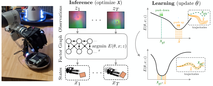
Instead of differentiating through the optimization process, we note that what we ultimately care about is the final solution from the optimizer, which depends only on the shape of the optimized cost function. We would like a cost function that has low cost around the observed ground truth trajectories and high cost elsewhere. This is precisely what energy-based models aim to do by shaping an “energy” function to be low around observed data and high elsewhere [14, 15, 16]. We cast our problem of learning observation models for estimation as energy-based learning.
We propose a novel approach, Learning Energy-based Models in Factor Graph Optimization (LEO), for learning observation models end-to-end with graph optimizers that may be non-differentiable. LEO alternates between sampling trajectories from the graph posterior and updating the model to match the distribution of samples to ground truth trajectories. We show that we can generate such samples efficiently using incremental Gauss-Newton graph solvers that create a Gaussian approximation for the Boltzmann distribution defined over a continuous space of trajectories. To the best of our knowledge, this is the first paper to show that even non-differentiable factor graph models can be learned efficiently. Our main contributions are:
- 1.
A novel formulation of learning observation models in estimation as energy-based learning.
- 2.
An algorithm, LEO, to learn observation models that minimize end-to-end tracking errors in factor graph optimizers that may be non-differentiable.
- 3.
Empirical evaluation on two distinct tasks: synthetic navigation and real-world planar pushing.
2 Related Work
Filtering and smoothing based estimation. Observation models represent joint or conditional distributions between states and measurements. Early estimation methods utilized these models within filtering contexts such as Kalman filters and EKFs/UKFs [17, 18]. Recent methods have also looked at making these filters differentiable for end-to-end learning [19, 20, 21, 22, 23, 24]. However, filtering can be inconsistent for nonlinear estimation problems due to linearization based on past, marginalized states that cannot be undone [25]. Instead, problems in simultaneous localization and mapping (SLAM) are increasingly formulated as smoothing or nonlinear optimization objectives [3, 2, 1]. Unlike filtering, smoothing allows dynamic relinearization of past states as well as exploits the inherent sparsity resulting in efficient and more accurate solutions. Factor graphs are an increasingly popular way for solving such smoothing problems [1, 2, 4, 5, 8, 26, 27, 28, 29], offering a flexible modeling framework while being efficient to optimize. We use the factor graph based smoothing framework in this paper.
Learning for smoothing. Typically, observation models used in factor graphs are analytic models defined a-priori [30, 31, 32]. Recent work has looked at using learned models [4, 5, 6] or learned measurement representations [27, 33] either to be used independently or to be plugged into a graph optimizer. However, these model parameters are learned on surrogate losses independent of the graph optimizer, and hence do not directly attempt to minimize final tracking errors.
An alternative approach is to view observation model parameters as hyper-parameters of the graph and perform a hyper-parameter search. This is usually done as sampling and derivative-free approaches using black-box solvers [11, 12, 13]. However, the high computational burden associated with sampling and evaluation can be prohibitive for large parameter spaces.
Differentiable optimization. Instead of a search, one may learn these model parameters via a continuous gradient-based optimizer matching graph optimizer output against a desired solution. Minimizing this loss would, however, require differentiating through the argmin optimization process. One way to do this is via unrolling where the optimization is represented as a series of differentiable, gradient based updates [16, 34, 35]. Since smoothing is a nonlinear least-squares optimization, it too can be unrolled in a similar fashion via differentiable Levenberg-Marquardt updates [9, 36, 37] or differentiable Gauss-Newton updates [8, 38, 39]. However, vanilla unrolling suffers from some drawbacks, notably the learned cost function can be sensitive to the specific optimization procedure, e.g. number of unrolling steps [40]. Moreover, this approach cannot be readily applied to commonly used optimizers relying on non-differentiable heuristics such as those in GTSAM, SNOPT [41, 42]. An alternate to unrolling is to employ the implicit function theorem which states that an optimal energy function must satisfy first-order necessary conditions [43, 44]. While this is promising for convex problems, for non-convex problems, one may recover an energy function with multiple minima such that the optimizer at test time may find itself in a different basin from ground truth.
Energy-based learning. Instead of differentiating through the optimization process, we note what we ultimately care about is the final solution from the optimizer, which depends only on the shape of the cost function. This is what energy-based models aim to do by shaping an “energy” function to be low around observed data and high elsewhere [14]. Energy-based modeling is a family of unsupervised learning methods popular in many structured prediction tasks such as inverse reinforcement learning [45, 46, 47, 48] and computer vision [49, 50]. Recently, a number of approaches have looked at training deep energy-based models [51, 52, 16]. The challenge with such methods is generating samples from the energy based model. Methods either rely on MCMC sampling [53, 54, 55] which does not scale well with dimension or resort to learning a separate generator [56, 57, 15]. We propose a way to generate such samples efficiently using incremental Gauss-Newton solvers. Recent work [58, 59] has also looked at learning observation models using variational inference techniques when ground truth states are not available. However, in our work, we can assume some ground truth demonstrations from a motion capture system which makes the problem more tractable.
3 Problem Formulation
We formalize our problem of learning observation models under the general theoretical framework of energy based models. We begin by describing the observation model, how it is optimized at inference time and finally how its parameters are learned from training data (Fig. 1).
3.1 Model
We define an energy-based model that captures dependencies between variables in a graph by associating a scalar energy to each configuration of the graph. Our goal is to model the likelihood of a sequence of latent states given a sequence of measurements . We adopt a factor graph framework (Fig. 1(a)) for expressing this likelihood as22 2 We use the word likelihood as in typical learning formulations. Specifically, it refers to the posterior of states given measurements. Model parameters include covariances in the norm as well.,
| (1) |
where, is the sequence of latent states, and is the sequence of measurements. are the factor costs with being the local observation model mapping a subset of states and measurements to a cost, are the learnable model parameters, and is the normalization or partition function.
Note that Eq. 1 is a special case of the Boltzmann distribution where the energy is a sum-of-squares. Notably, when is linearized, is quadratic in and subsequently becomes a Gaussian distribution. This is the structure that Gauss-Newton solvers employ, and we will leverage this fact to efficiently sample trajectories as described later in Section 4.3.
3.2 Inference
At inference time, given a sequence of measurements , we wish to solve for the most likely sequence of latent states . We formulate this as maximizing the log-likelihood of the model,
| (2) |
Substituting the model expression from Eq. 1, and dropping constants and , results in a nonlinear least-squares minimization of the form,
| (3) |
We use an efficient online Gauss-Newton graph solver for this objective. This enables both real-time inference as well as efficient sampling for learning model parameters during training (Section 4.3).
3.3 Learning
At train time, our goal is to learn a model that explains training data of pairs . We express this as minimizing a loss over the training data
| (4) |
where, is a training dataset of ground truth trajectories and measurements.
There are various choices of losses for learning model parameters ,
Loss 1: Minimize final tracking loss. A straightforward choice for is to directly minimize final tracking errors between optimized and ground truth trajectories, i.e. . While this loss directly minimizes final tracking errors, it may not be differentiable since the graph inference path from to is not differentiable. In such cases, we are limited to black-box hyperparameter search which is very sample inefficient.
Loss 2: Minimize surrogate loss. An alternate choice for the loss is to directly map measurements to ground truth states, for example as a regression or classification problem. Such a surrogate loss is independent of graph inference, and unlike Loss 1, is differentiable and easy to optimize. However, this does not minimize the final tracking errors that we care about.
Loss 3: Minimize energy-based loss. Finally, we consider a loss that is a function of the energy, i.e. . Intuitively, this assigns a low loss to well-behaved energy functions, i.e. functions that give the lowest energy to training data of ground truth trajectories (correct answers) and higher energy to unseen data (incorrect answers).
This energy-based loss, unlike Loss 2, is highly correlated with the final tracking loss as it shapes the energy (or cost) landscape so as to make the inference step return trajectories closer to the ground truth. Moreover, unlike Loss 1, this loss is only a function of energies which is differentiable irrespective of inference. Hence, we use Loss 3 and detail our approach in the next section.
4 Approach
We instantiate the broad framework of energy-based learning within the context of factor graph estimation in 4.1 and 4.2. In 4.3 we show how incremental Gauss Newton approaches enable efficient sampling from these energy based models.
4.1 Normalized Negative Log-Likelihood Loss
We define the overall loss as the negative log-likelihood (NLL) of the data under the energy model33 3 The motivation for NLL loss comes from probabilistic modeling, notably maximum entropy moment matching. We provide a detailed derivation along with its Gaussian approximation in Appendix C.:
| (5) |
Substituting as the Boltzman distribution expression from Eq. 1 we have,
| (6) |
The expression above has an intuitive explanation. The first term penalizes high energy over ground truth training samples. The second term penalizes low energy everywhere else, thus acting as a “contrastive” term. This has a desirable effect of globally shaping the energy function so that the minima lies at the training samples. The contrastive term prevents the energy surface from becoming flat and thus degenerate [14]. Unfortunately, we cannot directly plug in Eq. 6 as a standard machine learning loss (e.g. in PyTorch) to optimize. This is because the second log partition term is over a continuous space of trajectories , which renders exact computation intractable for arbitrary nonlinear cost functions [60].
Instead, let us take the gradient of this loss, and substitute expression from Eq. 1,
| (7) |
We see the log partition term transforms into an expectation over the learned distribution. The gradient expression above has a similar interpretation as the loss. The first term pushes down the energy of ground truth training samples. Interestingly, the second term now pulls up the energy of samples drawn from the learned Boltzmann distribution. If one is able to generate such samples, computing the gradient is straightforward.
Generally, sampling from the continuous Boltzmann distribution is intractable, relying typically on MCMC methods. But as we will detail in Section 4.3, we can indeed generate such samples efficiently since our graph optimizer maintains a Gaussian approximation of this distribution. Additionally in practice, we found that introducing a temperature term inside the Boltzmann distribution, i.e. , was critical for controlling the variance of the samples. Setting corresponds to only using the mode of the distribution which in this case is the mean trajectory. This corresponds to minimizing a generalized perceptron loss [14].
4.2 LEO Algorithm
Algorithm 1 summarizes the LEO algorithm, also illustrated in Fig. 2. It takes as inputs the training data containing ground truth state and measurement pairs, i.e. , , along with initial values for the learnable observation model parameters . The goal is to converge to a that minimizes the log-likelihood loss in Eq. 5 over the given training set .
LEO invokes a black-box, non-differentiable graph optimizer iSAM2 in the loop to generate samples. Within each LEO iteration, for every training example , we invoke the graph optimizer to obtain a Gaussian approximation to the original Boltzmann distribution about its mode. We then sample trajectories from this distribution.
The next step is to compute gradients of the energy, i.e. and , at the ground truth and the samples , respectively. Note that the gradients here are only w.r.t. , and not , and hence do not require the graph optimizer to be differentiable. Once we have the two gradients, we use the difference between them to update the observation model parameters . These updated parameters are then used in the next LEO iteration.
4.3 Efficient Inference via Incremental Gauss-Newton
The only thing that remains to be specified in Algorithm 1 is — How do we generate samples efficiently from the graph inference? In Section 3.2 we noted that our inference algorithm must satisfy two requirements (a) real-time inference and (b) sampling from the Boltzmann distribution. We achieve this using via incremental Gauss-Newton to solve the nonlinear least squares in Eq. 3.
Gauss-Newton proceeds by linearizing observation model functions about a point ,
| (8) |
where, is the linearization point, is the measurement Jacobian, and the state update vector. Measurements and learnable parameters are treated as constant within the graph optimization step. Substituting the Taylor expansion in Eq. 8 back into Eq. 3,
| (9) |
where, , are constructed by concatenating all , together into a single matrix and vector respectively. We then iterate until convergence.
We can solve for the objective in Eq. 9 efficiently by exploiting two properties of the problem: sparsity and online measurements. For SLAM problems, both and are large but sparse matrices, and can hence be factorized efficiently using sparse QR or Cholesky factorization respectively [61]. However, this still does not guarantee real-time inference during test time since grows with measurements over time, making the method increasingly slower. Instead, subsequent incremental solvers [10, 62, 63] reuse matrix factorizations from previous time steps. In this work, we use iSAM2 [10], an incremental Gauss-Newton graph solver whose resulting MAP solution can be expressed as a Gaussian probability distribution with mean and covariance,
| (10) |
This is the Gaussian approximation of the original Boltzmann distribution which we can now sample from efficiently. The graph posterior covariance for such a Gauss-Newton solver is obtained using just Jacobians without needing to compute a Hessian [2]. Note that sampling is done at the tangent space of the linearized graph, i.e. where and is a retraction [64]. The Gauss-Newton method for inference is an efficient technique for sampling from intractable models. A recent overview of the Laplace approximation with Gauss-Newton method can be found in [65]. Here, we build a specific Laplace approximation using the incremental solver iSAM2 that scales to sampling efficiently in real-time from very large graphs.44 4 See Appendix B for run time comparison to an alternate MCMC sampler.
5 Results and Evaluation
We evaluate LEO on synthetic navigation and real-world planar pushing. We compare against baselines on metrics like final tracking error and sample efficiency. We implement LEO in PyTorch [66] and interface it with the GTSAM C++ library [41], which contains several factor graph optimizers. We use the iSAM2 [10] optimizer for real-time, online optimization.

5.1 Overview
Experimental setup: For synthetic navigation (Datasets N1–N4), the goal is to estimate latent robot poses from relative odometry and absolute GPS measurements. For real-world planar pushing (Datasets P1–P3), the goal is to estimate latent object poses from tactile image measurements using a DIGIT tactile sensor [67] as shown in the setup in Fig. 3. Both these problems are modeled as factor graphs with poses as variable nodes and measurements as factor nodes.
Observation model parameters: Recall factor costs are defined by the local observation model and learned model parameters . Since we use Gaussian factors, we will learn their mean and covariance parameters, . For the navigation task, we learn (a) fixed covariances (N1, N2), and (b) covariances as a function of measurements (N3, N4). For the planar pushing task, we learn (a) fixed covariances (P1, P2), and (b) means as a function of tactile image measurements (P3). For all experiments, we use a diagonal covariance model.
Baselines: We compare against a learned sequence model such as LSTM, and black-box hyperparameter search methods such as CMAES [11] and Nelder-Mead, all of which optimize Loss 1. We also compare against a surrogate supervised learning method [4] which optimizes Loss 2.
Appendix D contains more details on the experimental setup, factor graph models, and results.

5.2 End-to-end Tracking Errors
Fig. 4 shows final tracking results for navigation datasets. We initialize LEO with random such that the graph optimizer returns trajectories far from the ground truth. At the final iteration, LEO converges to a that matches the optimized trajectories to ground truth. We summarize quantitative performance against baselines minimizing final tracking loss (Loss 1). LEO consistently outperforms baselines on final rmse tracking errors. The difference is more pronounced for datasets N3, N4 where the varying covariance model has a higher dimensional parameter space.
Fig. 5 shows final tracking results for real-world planar pushing datasets. Similar to navigation, we show LEO converging to ground truth trajectory for two different objects, a rectangle and ellipse, with differing local contact patches. We report quantitative performance on datasets P1, P2. LEO outperforms different hand-tuned choices of covariances as used in prior work [4].

5.3 Sample Efficiency and Convergence
Black-box hyper-parameter search is sample inefficient and does not scale well with increasing dimensionality. LEO, on the other hand, is efficient as it uses gradients. This can be seen in Fig. 4, where LEO consistently has lower graph optimizer calls (fevals). Moreover, LEO can also be used to learn models with larger parameter spaces, e.g. Fig. 7 learns parameters for a tactile factor neural network mapping keypoint image features to transformations (Fig. 3).
Finally, Fig. 6 shows LEO consistently converging for varying initializations on navigation dataset N1. We further show how the LEO samples evolve over iterations. Initially, when the cost is incorrect, the samples are more spread out. Over iterations, as the cost converges, the samples concentrate about the ground truth trajectory.


5.4 Surrogate Loss Analysis
We further analyze why a surrogate loss (Loss 2), independent of the graph optimizer, may not minimize end-to-end tracking errors. We train a network on surrogate supervised learning loss to directly map a pair of tactile image features to ground truth poses similar to prior work [4]. Fig. 7(b) shows the per time step surrogate loss on two trajectories — an initial trajectory that deviates from ground truth, and a final converged trajectory. While the tracking errors of final is much less than initial, the surrogate loss does not strictly improve. This is further reflected in the table in Fig. 7(c) where the surrogate loss baseline has higher final tracking errors over LEO for dataset P1.
6 Conclusion
We presented an approach, LEO, for learning observation models end-to-end with graph optimizers that may be non-differentiable. We compared LEO against baselines for different observation model types on two distinct tasks of navigation and real-world planar pushing. Overall, LEO is able to learn observation models with lower errors and fewer samples. While we investigated LEO with non-differentiable optimizers in this paper, as future work, we would like to apply LEO to differentiable optimizers and compare against alternate solutions such as unrolling (see Appendix A for a more detailed discussion). We would also like to scale to more complex observation models with applications to 3D object tracking using tactile sensors.
Acknowledgements
This work was supported through the FRAIM program. We thank Frank Dellaert for insightful feedback and suggestions on the paper.
References
- Dellaert [2020] F. Dellaert. Factor graphs: Exploiting structure in robotics. Annual Review of Control, Robotics, and Autonomous Systems, 4, 2020.
- [2] F. Dellaert and M. Kaess. Factor graphs for robot perception. Foundations and Trends in Robotics.
- Cadena et al. [2016] C. Cadena, L. Carlone, H. Carrillo, Y. Latif, D. Scaramuzza, J. Neira, I. Reid, and J. J. Leonard. Past, present, and future of simultaneous localization and mapping: Toward the robust-perception age. IEEE Trans. Robotics, 2016.
- Sodhi et al. [2021] P. Sodhi, M. Kaess, M. Mukadam, and S. Anderson. Learning tactile models for factor graph-based estimation. In IEEE Intl. Conf. on Robotics and Automation (ICRA), 2021.
- Baikovitz et al. [2021] A. Baikovitz, P. Sodhi, M. Dille, and M. Kaess. Ground encoding: Learned factor graph-based models for localizing ground penetrating radar. In IEEE/RSJ Intl. Conf. on Intelligent Robots and Systems (IROS), 2021.
- Sundaralingam et al. [2019] B. Sundaralingam, A. S. Lambert, A. Handa, B. Boots, T. Hermans, S. Birchfield, N. Ratliff, and D. Fox. Robust learning of tactile force estimation through robot interaction. In IEEE Intl. Conf. on Robotics and Automation (ICRA), 2019.
- Lambert et al. [2018] A. Lambert, A. Shaban, A. Raj, Z. Liu, and B. Boots. Deep forward and inverse perceptual models for tracking and prediction. In IEEE Intl. Conf. on Robotics and Automation (ICRA), pages 675–682, 2018.
- Yi et al. [2021] B. Yi, M. Lee, A. Kloss, R. Martín-Martín, and J. Bohg. Differentiable factor graph optimization for learning smoothers. arXiv preprint arXiv:2105.08257, 2021.
- Jatavallabhula et al. [2020] K. M. Jatavallabhula, G. Iyer, and L. Paull. GradSLAM: Dense SLAM meets automatic differentiation. In IEEE Intl. Conf. on Robotics and Automation (ICRA), 2020.
- Kaess et al. [2012] M. Kaess, H. Johannsson, R. Roberts, V. Ila, J. Leonard, and F. Dellaert. iSAM2: Incremental smoothing and mapping using the Bayes tree. Intl. J. of Robotics Research, 31(2):216–235, Feb. 2012.
- Hansen et al. [2019] N. Hansen, Y. Akimoto, and P. Baudis. CMA-ES/pycma on Github. Zenodo, DOI:10.5281/zenodo.2559634, 2019. URL https://doi.org/10.5281/zenodo.2559634.
- Hu and Kantor [2015] H. Hu and G. Kantor. Parametric covariance prediction for heteroscedastic noise. In IEEE/RSJ Intl. Conf. on Intelligent Robots and Systems (IROS), 2015.
- Snoek et al. [2012] J. Snoek, H. Larochelle, and R. P. Adams. Practical bayesian optimization of machine learning algorithms. arXiv preprint arXiv:1206.2944, 2012.
- LeCun et al. [2006] Y. LeCun, S. Chopra, R. Hadsell, M. Ranzato, and F. Huang. A tutorial on energy-based learning. Predicting structured data, 1(0), 2006.
- Kumar et al. [2019] R. Kumar, S. Ozair, A. Goyal, A. Courville, and Y. Bengio. Maximum entropy generators for energy-based models. arXiv preprint arXiv:1901.08508, 2019.
- Belanger et al. [2017] D. Belanger, B. Yang, and A. McCallum. End-to-end learning for structured prediction energy networks. In International Conference on Machine Learning (ICML), 2017.
- Julier and Uhlmann [2004] S. J. Julier and J. K. Uhlmann. Unscented filtering and nonlinear estimation. Proceedings of the IEEE, 92(3):401–422, 2004.
- Thrun et al. [2001] S. Thrun, D. Fox, W. Burgard, and F. Dellaert. Robust Monte Carlo localization for mobile robots. Artificial intelligence, 128(1-2):99–141, 2001.
- Kloss et al. [2020] A. Kloss, G. Martius, and J. Bohg. How to train your differentiable filter. arXiv preprint arXiv:2012.14313, 2020.
- Lee et al. [2020] M. A. Lee, B. Yi, R. Martín-Martín, S. Savarese, and J. Bohg. Multimodal sensor fusion with differentiable filters. In IEEE/RSJ Intl. Conf. on Intelligent Robots and Systems (IROS), 2020.
- Jonschkowski et al. [2018] R. Jonschkowski, D. Rastogi, and O. Brock. Differentiable particle filters: End-to-end learning with algorithmic priors. arXiv preprint arXiv:1805.11122, 2018.
- Venkatraman et al. [2017] A. Venkatraman, N. Rhinehart, W. Sun, L. Pinto, M. Hebert, B. Boots, K. Kitani, and J. Bagnell. Predictive-state decoders: Encoding the future into recurrent networks. Advances in Neural Information Processing Systems, 30, 2017.
- Sun et al. [2016] W. Sun, A. Venkatraman, B. Boots, and J. A. Bagnell. Learning to filter with predictive state inference machines. In International Conference on Machine Learning (ICML), 2016.
- Haarnoja et al. [2016] T. Haarnoja, A. Ajay, S. Levine, and P. Abbeel. Backprop kf: Learning discriminative deterministic state estimators. In Advances in Neural Information Processing Systems 24 (NeurIPS), 2016.
- Julier and Uhlmann [2001] S. J. Julier and J. K. Uhlmann. A counter example to the theory of simultaneous localization and map building. In IEEE Intl. Conf. on Robotics and Automation (ICRA), volume 4, pages 4238–4243, 2001.
- Ortiz et al. [2021] J. Ortiz, T. Evans, and A. J. Davison. A visual introduction to gaussian belief propagation. arXiv preprint arXiv:2107.02308, 2021.
- Czarnowski et al. [2020] J. Czarnowski, T. Laidlow, R. Clark, and A. J. Davison. DeepFactors: Real-time probabilistic dense monocular SLAM. IEEE Robotics and Automation Letters, 2020.
- Hartley et al. [2018] R. Hartley, M. G. Jadidi, L. Gan, J.-K. Huang, J. W. Grizzle, and R. M. Eustice. Hybrid contact preintegration for visual-inertial-contact state estimation using factor graphs. In IEEE/RSJ Intl. Conf. on Intelligent Robots and Systems (IROS), pages 3783–3790, 2018.
- Fourie et al. [2016] D. Fourie, J. Leonard, and M. Kaess. A nonparametric belief solution to the bayes tree. In IEEE/RSJ Intl. Conf. on Intelligent Robots and Systems (IROS), 2016.
- Mur-Artal and Tardós [2017] R. Mur-Artal and J. D. Tardós. ORB-SLAM2: An open-source SLAM system for monocular, stereo, and RGB-D cameras. IEEE Trans. Robotics, 33(5):1255–1262, 2017.
- Engel et al. [2014] J. Engel, T. Schöps, and D. Cremers. LSD-SLAM: Large-scale direct monocular SLAM. In Eur. Conf. on Computer Vision (ECCV), pages 834–849. Springer, 2014.
- Lambert et al. [2019] A. S. Lambert, M. Mukadam, B. Sundaralingam, N. Ratliff, B. Boots, and D. Fox. Joint inference of kinematic and force trajectories with visuo-tactile sensing. In IEEE Intl. Conf. on Robotics and Automation (ICRA), pages 3165–3171, 2019.
- Bloesch et al. [2018] M. Bloesch, J. Czarnowski, R. Clark, S. Leutenegger, and A. J. Davison. CodeSLAM–learning a compact, optimisable representation for dense visual slam. In Proc. IEEE Int. Conf. Computer Vision and Pattern Recognition, 2018.
- Wilder et al. [2019] B. Wilder, E. Ewing, B. Dilkina, and M. Tambe. End to end learning and optimization on graphs. Advances in Neural Information Processing Systems, 32:4672–4683, 2019.
- Bechtle et al. [2021] S. Bechtle, A. Molchanov, Y. Chebotar, E. Grefenstette, L. Righetti, G. Sukhatme, and F. Meier. Meta learning via learned loss. In 2020 25th International Conference on Pattern Recognition (ICPR), 2021.
- Lv et al. [2019] Z. Lv, F. Dellaert, J. M. Rehg, and A. Geiger. Taking a deeper look at the inverse compositional algorithm. In Proc. IEEE Int. Conf. Computer Vision and Pattern Recognition, 2019.
- Tang and Tan [2018] C. Tang and P. Tan. Ba-net: Dense bundle adjustment networks. In International Conference on Learning Representations (ICLR), 2018.
- von Stumberg et al. [2020] L. von Stumberg, P. Wenzel, Q. Khan, and D. Cremers. Gn-net: The gauss-newton loss for multi-weather relocalization. IEEE Robotics and Automation Letters, 5(2):890–897, 2020.
- Bhardwaj et al. [2020] M. Bhardwaj, B. Boots, and M. Mukadam. Differentiable Gaussian process motion planning. In IEEE Intl. Conf. on Robotics and Automation (ICRA), 2020.
- Amos and Yarats [2020] B. Amos and D. Yarats. The differentiable cross-entropy method. In International Conference on Machine Learning, pages 291–302. PMLR, 2020.
- Dellaert [2012] F. Dellaert. Factor graphs and GTSAM: A hands-on introduction. Technical report, Georgia Institute of Technology, 2012.
- Gill et al. [2005] P. E. Gill, W. Murray, and M. A. Saunders. SNOPT: An SQP algorithm for large-scale constrained optimization. SIAM review, 47(1):99–131, 2005.
- Dontchev and Rockafellar [2009] A. L. Dontchev and R. T. Rockafellar. Implicit functions and solution mappings, volume 543. Springer, 2009.
- Amos and Kolter [2017] B. Amos and J. Z. Kolter. Optnet: Differentiable optimization as a layer in neural networks. In International Conference on Machine Learning (ICML), pages 136–145, 2017.
- Ziebart et al. [2008] B. D. Ziebart, A. L. Maas, J. A. Bagnell, and A. K. Dey. Maximum entropy inverse reinforcement learning. In AAAI Conf. on Artificial Intelligence, volume 8, pages 1433–1438, 2008.
- Du et al. [2019] Y. Du, T. Lin, and I. Mordatch. Model based planning with energy based models. arXiv, 2019.
- Wulfmeier et al. [2015] M. Wulfmeier, P. Ondruska, and I. Posner. Maximum entropy deep inverse reinforcement learning. arXiv preprint arXiv:1507.04888, 2015.
- Kitani et al. [2012] K. M. Kitani, B. D. Ziebart, J. A. Bagnell, and M. Hebert. Activity forecasting. In Eur. Conf. on Computer Vision (ECCV), 2012.
- Gustafsson et al. [2020] F. K. Gustafsson, M. Danelljan, R. Timofte, and T. B. Schön. How to train your energy-based model for regression. In British Machine Vision Conf. (BMVC), 2020.
- Du et al. [2020] Y. Du, S. Li, J. Tenenbaum, and I. Mordatch. Improved contrastive divergence training of energy based models. arXiv preprint arXiv:2012.01316, 2020.
- Chen et al. [2015] L.-C. Chen, A. Schwing, A. Yuille, and R. Urtasun. Learning deep structured models. In International Conference on Machine Learning (ICML), 2015.
- Belanger and McCallum [2016] D. Belanger and A. McCallum. Structured prediction energy networks. In International Conference on Machine Learning (ICML), 2016.
- Tieleman [2008] T. Tieleman. Training restricted boltzmann machines using approximations to the likelihood gradient. In International Conference on Machine Learning (ICML), pages 1064–1071, 2008.
- Du and Mordatch [2019] Y. Du and I. Mordatch. Implicit generation and modeling with energy based models. In Advances in Neural Information Processing Systems 24 (NeurIPS), 2019.
- Nijkamp et al. [2019] E. Nijkamp, M. Hill, S.-C. Zhu, and Y. N. Wu. Learning non-convergent non-persistent short-run mcmc toward energy-based model. In Advances in Neural Information Processing Systems 24 (NeurIPS), 2019.
- Kim and Bengio [2016] T. Kim and Y. Bengio. Deep directed generative models with energy-based probability estimation. arXiv preprint arXiv:1606.03439, 2016.
- Dai et al. [2017] Z. Dai, A. Almahairi, P. Bachman, E. Hovy, and A. Courville. Calibrating energy-based generative adversarial networks. arXiv preprint arXiv:1702.01691, 2017.
- Yoon et al. [2021] D. J. Yoon, H. Zhang, M. Gridseth, H. Thomas, and T. D. Barfoot. Unsupervised learning of lidar features for use ina probabilistic trajectory estimator. IEEE Robotics and Automation Letters, 6(2), 2021.
- Wong et al. [2020] J. N. Wong, D. J. Yoon, A. P. Schoellig, and T. D. Barfoot. Variational inference with parameter learning applied to vehicle trajectory estimation. IEEE Robotics and Automation Letters, 5(4), 2020.
- Wainwright et al. [2005] M. J. Wainwright, T. S. Jaakkola, and A. S. Willsky. A new class of upper bounds on the log partition function. IEEE Transactions on Information Theory, 51(7):2313–2335, 2005.
- Dellaert and Kaess [2006] F. Dellaert and M. Kaess. Square root SAM: Simultaneous localization and mapping via square root information smoothing. Intl. J. of Robotics Research, 2006.
- Kaess et al. [2008] M. Kaess, A. Ranganathan, and F. Dellaert. iSAM: Incremental smoothing and mapping. IEEE Trans. Robotics, 24(6):1365–1378, 2008.
- Sodhi et al. [2020] P. Sodhi, S. Choudhury, J. G. Mangelson, and M. Kaess. ICS: Incremental constrained smoothing for state estimation. In IEEE Intl. Conf. on Robotics and Automation (ICRA), 2020.
- Sola et al. [2018] J. Sola, J. Deray, and D. Atchuthan. A micro lie theory for state estimation in robotics. arXiv preprint arXiv:1812.01537, 2018.
- Immer et al. [2021] A. Immer, M. Korzepa, and M. Bauer. Improving predictions of bayesian neural nets via local linearization. In International Conference on Artificial Intelligence and Statistics, pages 703–711. PMLR, 2021.
- Paszke et al. [2019] A. Paszke, S. Gross, F. Massa, A. Lerer, J. Bradbury, G. Chanan, T. Killeen, Z. Lin, N. Gimelshein, L. Antiga, A. Desmaison, A. Kopf, E. Yang, Z. DeVito, M. Raison, A. Tejani, S. Chilamkurthy, B. Steiner, L. Fang, J. Bai, and S. Chintala. PyTorch: An imperative style, high-performance deep learning library. In Advances in Neural Information Processing Systems 24 (NeurIPS), pages 8024–8035, 2019.
- Lambeta et al. [2020] M. Lambeta, P.-W. Chou, S. Tian, B. Yang, B. Maloon, V. R. Most, D. Stroud, R. Santos, A. Byagowi, G. Kammerer, et al. DIGIT: A novel design for a low-cost compact high-resolution tactile sensor with application to in-hand manipulation. IEEE Robotics and Automation Letters, 5(3):3838–3845, 2020.
- [68] https://github.com/borglab/SwiftFusion.
- Package Contributors and Ecosystem [2021] Package Contributors and Ecosystem. Caesar.jl, v0.10.2, 2021. https://github.com/JuliaRobotics/Caesar.jl.
- Cobb and Jalaian [2021] A. D. Cobb and B. Jalaian. Scaling hamiltonian monte carlo inference for bayesian neural networks with symmetric splitting. Uncertainty in Artificial Intelligence, 2021. https://github.com/AdamCobb/hamiltorch.
- Jaynes [1957] E. T. Jaynes. Information theory and statistical mechanics. Physical review, 106(4), 1957.
- Ziebart [2010] B. D. Ziebart. Modeling purposeful adaptive behavior with the principle of maximum causal entropy. PhD thesis, 2010.
- Levine et al. [2011] S. Levine, Z. Popovic, and V. Koltun. Nonlinear inverse reinforcement learning with Gaussian processes. In Advances in Neural Information Processing Systems 24 (NeurIPS), 2011.
- Finn et al. [2016] C. Finn, P. Christiano, P. Abbeel, and S. Levine. A connection between generative adversarial networks, inverse reinforcement learning, and energy-based models. arXiv preprint arXiv:1611.03852, 2016.
Appendix
Appendix A Applying LEO to Differentiable Optimizers
We discuss here how LEO can be applied to differentiable optimization libraries. It requires two simple changes, (a) disable gradients from the inner loop optimizer block, and (b) replace the direct final tracking loss (Loss 1) with an energy-based loss (Loss 3). To illustrate how LEO performs compared to alternate solutions such as unrolling, we choose the uni-dimensional regression task from [40]. This enables us to visualize the learned 2D energy surfaces.
Setup In the regression task, the goal is to learn a network that maps points to an energy value, given samples from a ground truth function. The ground truth data is generated from the function for . We model where . is the energy function expressed as a sum-of-squares of , similar to Section 3.1, to apply Gauss-Newton solvers. is modeled as a neural network with as the learnable network parameters.
LEO minimizes an energy-based loss (Loss 3), i.e. , resulting in a similar update rule of the form,
| (11) |
We solve for this update using the Adam optimizer in Pytorch. We use a batch Gauss-Newton solver as our underlying inner loop optimizer (LEO GN).
The unrolling baselines minimize a final tracking loss (Loss 1), i.e. , where . We use both unrolled gradient descent (Unrolled GD) and unrolled Gauss-Newton (Unrolled GN) [8].
For all methods, we use two initialization schemes for the underlying optimizer. The first scheme initializes from for all , as followed in [40]. The second scheme initializes from the ground truth as suggested in [8].


Results Fig. 8 shows the learned energy surfaces for all 3 methods using initialization scheme 1, i.e., initializing the optimizer from zero. At iteration , all 3 approaches are initialized with a random energy function. While all 3 approaches end up with a low final loss, only LEO converges to an energy function with a single basin about the ground truth samples. The unrolled baselines converge to energy functions with multiple minima, not all of them on the ground truth samples. This is because the energy function need only be good enough for the optimizer, when initialized from to reach the ground truth for a fixed number of unrolling steps. It does not guarantee a similar convergence when executed with different number of unrolling steps or initialization from different values.
Fig. 9 shows the learned energy surfaces for initialization scheme 2, i.e., initializing the optimizer from ground truth. Similar to the previous figure, all 3 methods initialize from random energy functions and converge to a low final loss. But only LEO converges to a similar energy function as before, i.e., one with a single basin around the ground truth. The unrolling baselines converge to a different energy function than in scheme 1. In this case, the energy function need only be good enough for the optimizer, when initialized from ground-truth, to stay on the ground truth.
For both schemes, LEO alone converges to the same energy function, as it is less sensitive to the underlying optimization process. In future work, we aim to apply LEO on differentiable optimizers for robot estimation tasks. This would require a factor graph optimization library similar to GTSAM but implemented in a differentiable manner. There are recent efforts on this front [8, 68, 69], but there isn’t a single, stable open-source library yet. We hope our analysis on this regression task would encourage others in the community to try out LEO in their respective differentiable optimizer libraries.
Appendix B Comparison to a MCMC sampler

We compare run times against an HMC sampler implemented in the hamiltorch library [70]. The sampler simulates a set of Hamiltonian differential equations which upon simulating generates a sequence of samples.
We run this on the 2D navigation dataset which have a 900-dimensional state space (3-DOF * 300 steps). The HMC sampler is sampling from the true posterior distribution while the incremental Gauss-Newton, iSAM2 [10], sampler that we use samples from a Gaussian approximation that it maintains online. However, we found similar convergence at train time using both samplers which suggests that the Gaussian approximation was reasonable for our applications.
In terms of run time, we found the HMC sampler run time to be two orders of magnitude greater than the iSAM2 sampler as shown in Fig. 10. This is expected since the HMC sampler evaluates the cost as well the gradients of the cost every time a sample is generated which requires looping through all the factors and can be expensive. In contrast, the iSAM2 sampler allows for directly sampling from the Gaussian that is significantly faster. When used in an online setting, as new factors get added to the graph, the HMC sampler would have to recompute the posterior distribution. On the other hand, the iSAM2 sampler efficiently and incrementally updates the Gaussian approximation by leveraging sparsity.
Appendix C Principle of Maximum Entropy
In Section 4.1, we defined the energy-based loss as the normalized negative log-likelihood loss. The motivation for such a loss comes from probabilistic modeling, notably the principle of maximum entropy moment matching.
Assume a ground truth distribution that generates x and z. We would like to estimate a distribution that matches this. The true ground truth distribution is unknown, but we can sample from it. This allows us to estimate by matching empirical moments computed from these samples (Fig. 11).
However, there is a continuous space of probability distributions that match these empirical moments. Which of these distributions do we pick? The maximum entropy (MaxEnt) principle suggests we pick the distribution which is least committal, i.e. the one with maximum entropy [71]. We can write out this objective of maximizing entropy of the distribution subject to matching moment constraints against the unknown ground truth distribution as,
| (12) |
where, are the moment functions. Applying KKT conditions for Eq. 12 and expanding the dual results in an unconstrained objective of the form [71, 72] (more details in Eq. 21),
| (13) |
where, are the Lagrange multipliers. The term can be interpreted as a linear “energy function” such that puts a high energy on low probability solutions. This linear class of cost functions can be lifted to a richer class of parametric nonlinear functions . Note that this may induce a duality gap in optimizing Eq. 12, but is commonly used in practice when parameterizing energy functions as neural networks [14, 73, 74]. The maximum entropy solution can then be written out as,
| (14) |
Eq. 14 asks us to maximize the likelihood of ground truth trajectories where the likelihood takes the form of a Boltzmann distribution, where lower energy implies higher probability mass. In other words, we want to find energy function that places maximal probability mass on the ground truth trajectory. Writing out this objective over a training dataset results in the NLL loss that we saw earlier in Section 4.1,
| (15) |
Let’s expand out the steps in Section 4.1 in more detail. Substituting the expression for Boltzmann distribution results in,
| (16) |
Take the gradient of this loss,
| (17) |
Substituting in from Section 3.1 we have the resulting gradient expression that we finally obtained in Section 4.1,
| (18) |
Negative log likelihood approximation
Since directly sampling from the true posterior is intractable, in LEO, we instead sample from a Gaussian approximation of this distribution, where , are obtained as shown in Section 4.3. Hence, we effectively minimize an approximation of the true NLL loss,
| (19) |
The difference between the approximated loss and the true loss is,
| (20) |
The difference in losses is bounded by the maximum log density ratio between the true and approximated distributions. The ratio is bounded as long as the denominator is not zero, i.e. the approximation has full support over the dataset.
Derivation from moment matching
When going from Eq. 12 to 13, we rewrote the constrained maximum entropy objective as an unconstrained objective. Let’s derive this for our setting [71]. For simplicity of notations, we’ll drop the conditional in the probability expressions.
We would like to maximize (or minimize negative) entropy subject to matching moments, i.e.,
| (21) |
Writing out the Lagrangian for this constrained problem,
| (22) |
where, , are the Lagrange multipliers. Taking gradient of Lagrangian and setting to ,
| (23) |
Eq. 23 goes to for a probability distribution of the form,
| (24) |
where, such that . We can subsume since that’s a constant.
Writing out the dual form of the Lagrangian with expression substituted from Eq. 24,
| (25) |
Introducing true distribution and rearranging terms results in the unconstrained objective that we saw in Eq. 13,
| (26) |
Appendix D Experimental Evaluation: Additional Details
D.1 Setup and Factor Graph Models
Fig. 12 shows the two factor graphs modeling the (a) synthetic navigation and (b) real-world planar pushing tasks. For both graphs, poses are modeled as variable nodes and measurements as factor nodes. The graph inference objective is to solve for the latent poses (variables) given measurements (factors).
Synthetic Navigation To replicate a typical robot navigation setup, we generate odometry measurements by adding Gaussian noise to relative ground truth state estimates and GPS measurements by adding Gaussian noise to absolute ground truth estimates. We generate 4 datasets N1–N4, each with a different covariance setting. N1, N2 has measurements generated from fixed covariances . N3, N4 has measurements generated from covariances varying between two sets of values, i.e. , where are binary measurements simulating an ambient light detector that determines whether the robot is in an indoor or outdoor environment.
To solve for the sequence of states from measurements , we provide the following objective for the graph optimizer to minimize,
| (27) |
The observation model parameters that we learn for this task are the fixed and varying covariances, i.e. .
Real-world planar pushing For the planar pushing setup, states in the graph are the planar object and end-effector poses at every time step, with , where . Factors in the graph incorporate tactile observations , quasi-static pushing dynamics , geometric constraints , and priors on end-effector poses .
To solve for the sequence of state from measurements , we pass in the following objective for the graph optimizer to minimize,
| (28) |
The observation model parameters that we learn for this task are the tactile factor network weights and the tactile and quasi-static factor covariances, i.e. . Tactile factor network contains an image to keypoint feature encoder pre-trained using a self-supervised image reconstruction loss and a fully connected network mapping keypoint features to relative transforms. We fine tune weights for the keypoint to relative transform portion of the network and use fixed, pre-trained weights for feature encoder. Tactile factors are added between non-consecutive poses over a window with the window length chosen heuristically, and quasi-static motion factors are added between consecutive poses (Fig. 12). More details on the factor graph models along with the network architecture can be found in prior work [4].

D.2 Baselines
For the hyper-parameter search baselines we use off-the-shelf solvers like CMA-ES [11], and scipy optimizers such as Nelder-Mead. For the learned sequence model baseline, we use an LSTM.
LSTM architecture For the synthetic navigation task, we directly regresses to absolute poses. At each time step, the absolute pose and odometry measurements are concatenated as inputs, and the network predicts the 2D position and the sin and cos of the rotation angle. We use a 2-layer LSTM with 64 hidden units, followed by a 2 dense layers of 32 hidden units before decoding into the 4D output. The loss is a weighted sum of translation and rotation errors. In the real-world planar pushing datasets, we do not have direct measurements of the object pose. Therefore, we transform all end-effector trajectories to start at the origin, which improves the generalization. Each input consists of the end-effector pose observation and the 2d object contact observation, and the same architecture as the navigation dataset is used. In addition, we found that increasing the sequence length with each epoch improved performance.
Fig. 13 shows qualitative results for the LSTM on the (a) synthetic navigation and (b) real-world planar pushing datasets. The performance on the planar pushing object trajectories is not as good since, unlike navigation where we had noisy GPS measurements, tactile measurements only give partially observable information about the object state.