A Method to use Nonlinear Dynamics in a Whisker Sensor for Terrain Identification by Mobile Robots
Abstract
This paper shows analytical and experimental evidence of using the vibration dynamics of a compliant whisker for accurate terrain classification during steady state motion of a mobile robot. A Hall effect sensor was used to measure whisker vibrations due to perturbations from the ground. Analytical results predict that the whisker vibrations will have a dominant frequency at the vertical perturbation frequency of the mobile robot sandwiched by two other less dominant but distinct frequency components. These frequency components may come from bifurcation of vibration frequency due to nonlinear interaction dynamics at steady state. Experimental results also exhibit distinct dominant frequency components unique to the speed of the robot and the terrain roughness. This nonlinear dynamic feature is used in a deep multi-layer perceptron neural network to classify terrains. We achieved 85.6% prediction success rate for seven flat terrain surfaces with different textures.
Index Terms:
Robotic whiskers, Surface identification, multi-layer perceptron, Modal analysis.I INTRODUCTION
Terrain surface identification is an important function for mobile robots moving and performing tasks in extreme,unstructured environments [1]. By identifying different terrain surfaces, mobile robots could better perceive the surrounding environment information and decide the optimal next move. For example, they can avoid less favorable terrain types such as soft sand, and use the identification information for mapping and localization objects. Although many sensors such as cameras are used for object recognition, whiskered tactile perception can potentially provide a robust, and economical solution for these problems, especially in extreme (e.g. dark, foggy) environments.

Over the years, vision [2], lidar [3], sound [4], inertial measurement units [5], and tactile sensors [6] have been studied for surface identification. Vision-based methods combined with deep learning have become a research hotspot and significant scientific and technological developments made. However, vision-based methods can have a high probability of failure because of the similar visual appearance of different terrains or objects. Moreover, visual accuracy is severely impaired by environmental conditions such as fog, smoke, low light levels, high-brightness and high-temperature. Recognition and classification methods for different objects based on lidar data have been popularly used in autonomous cars, but its accuracy will drop in sandy applications and dusty scenes. For an IMU installed on the mobile robot body, a challenge is that they cannot predict the terrain and object types in advance before the robot has contact. For example, when the robot detects a change in terrain from concrete to soft sand based on inertial signals, the wheels may have already come into contact with the sand. This can lead to dangerous consequences. Therefore, it is important to find robust sensing modes for the environment to achieve terrain identification under extreme unstructured environments and the whisker sensor is a choice worth exploring [7].
Artificial Whiskers sensors have been demonstrated in several studies that are a particularly high-efficiency method for animals such as rats and sea lions which can use them to navigate in the dark and perceive environmental information and features without vision [8].
This has motivated researchers to design and construct whiskers for applications such as navigation [9], obstacle avoidance [10], object detection [11], size measurement [12], shape recognization [13], and surface information [14]. For example, in [15], Zurek showed that static antennae can act as locomotory guides which can compensate for visual methods to determine the location and distance of obstacles during fast locomotion. By rotating the whisker against a sequence of contact points of the object and collecting torque information, Solomon and Hartmann put forward a method to obtain an object’s 3D contour information [16]. In 2020, authors of [17] showed that a novel variable stiffness controllable multi-modal whisker sensor can capture different vibration frequencies by controlling whisking speed and the stiffness of the follicle. In all these cases, experimental results prove that the whisker sensors can effectively compensate for the shortcomings of vision sensors in an extreme environment.
In the work reported here, we designed and constructed a novel whisker tactile sensor to achieve terrain identification for a mobile robot platform (Fig. 1). Reservoir computing [18, 19] is used in the whisker sensor to map slight changes in the ground perturbations to distinct steady state frequency components. This paper firstly shows that the steady state response of nonlinear vibration dynamics can be used to classify terrain textures even on flat terrain. The remainder of this paper is organized as follows: Section II introduces the design and construction of the whiskers tactile sensor, and the experimental system including the Raspberry robot, whiskered tactile sensor. The whisker sensor vibration characteristics and modal analysis are studied in Section III. Section IV reports the whisker vibration data collection and feature extraction as well as algorithm framework based on multi-layer perceptron. Section V presents the results and analysis of terrain identification experiments . Finally, Section VI concludes this paper’s contribution and discuss the future work.
II System Design & Preliminary Analysis
II-A Bioinspired Whisker Sensor Design
The proposed whiskered tactile sensor uses SS49E linear Hall sensors that are orthogonally mounted on one side of a silicone rubber sensor holder base and spring beam on the other side. The structure is shown in Figure 2. A neodymium permanent magnet is embedded inside the spring beam that is made of high-carbon steel, with the free length: 60 mm, wire diameter: 1 mm, outside diameter: 10 mm, and inside diameter: 8 mm respectively. Tapered silicone rubber is installed on the tip of the spring in order to accurately capture the vibration of the surface . The components and materials cost of this whiskered tactile sensor totalled less than $5 based on one-off non-discounted prices. The low cost construction of this novel sensor provides an advantage to many existing surface identification sensors

II-B Sensor Characterization & Working Principle
The whisker sensor is installed on the 4-DOF servo fusion rotating platform for orientation control of the whisker, which keeps the whisker sensor at a horizontal orientation all the time for clarity. When the robot traverses different terrain, external vibrations are applied to the whiskered spring shaft, and the shaft deforms also inducing the same vibrations on the magnet inside. This causes a continuous magnetic flux change near the linear hall effect sensor. Consequently, the hall effect sensor generates continuous low-frequency electrical voltage signals. The sensitivity of this whiskered tactile sensor relies on the vibration of the whiskered spring beam and the silicone rubber tip.
II-C Experimental Setup Design & Procedure
The experiment is conducted by a four-wheel mobile robot. The wheeled unit and electronic system are shown in Fig.1. The robot is 270 mm in length, 150 mm in height and 130 mm in width, 1.4 kg in mass, with the diameter and width of the wheels are 70 mm and 30 mm respectively. The robot car could traverse through the coarse ground at a speed of up to 1.3 m/s, With a power supply of 5 V.

The robot system consists of a whiskered tactile sensor orthogonal fixed in a 4-DOF servo fusion rotating platform, controlled by a Raspberry Pi 4 B.The whiskered tactile sensor has its own amplifier, and the raw voltage signals are sent to an ADS1115 analog to digital converter.
The AD converters, servo motor driver as well as the 4-DOF rotating platform are connected to a Raspberry Pi 4B. The sensor data collection, robot’s motion and rotating platform’s movement are synchronized controlled by the Raspberry Pi 4B . All data are recorded in the raspberry pi on-board flash memory, and then transferred to a computer (1.60 GHz, 8 GB RAM) via Bluetooth for processing. Fig.3 shows the system flow framework.
| (1) | |||||
III Preliminary Theoretical Study
The sensor vibration characteristics are studied as a proof-of-concept for the idea presented.
III-A Cantilever Beam Vibration with Base Excitation
The sensor is modelled as an equivalent cantilever beam with uniform mass under base excitation (Fig. 2). The steady state response of such system for sinusoidal base excitation can be found based on the derivations in [20] as a summation over the beam first five mode shapes in Eq. 1, where is the beam displacement at any length and time , and are the base excitation amplitude in [m] and frequency in [rad/s], is the base excitation frequency in [Hz], is a set of constants related to a cantilever beam mode shapes [20], and is the modal damping based on stainless steel material. The equivalent beam has a length similar to the coil spring axial length [mm] and cross-section area similar to the spring wire cross-section area , where [mm] is the wire radius. The beam unit length density is where [Kg/] is the wire material (stainless steel) density, and is a correction factor to account for the coil shape based on the spring wire pitch , overall length , and spring number of coils . We may assume that the beam bending modulus is equivalent to the spring wire torsional modulus , where [GPa] is the wire material (stainless steel) shear modulus, and is the wire cross-section moment of area.
III-B Sensor Modal Analysis

The simulation results for the sensor lateral displacement , where [mm] is the sensor distance from the beam base, and the signal FFT (Fast Fourier Transform) analysis in response to different excitation parameters ( [mm] and [Hz]) are plotted in Fig. 4. Distinctively different signal profiles and dominant frequency are observed for different excitation frequencies (i.e. due to ground texture). The signal dominant frequency is the same as the base excitation frequency.
Fig. 5 shows the sensor maximum displacement in [m] and dominant modal frequency in [Hz] for different excitation frequency and amplitude . It is observed that is similar to and does not vary with . This shows that it is possible to successfully classify the excitation frequency (i.e. ground profile texture) based on the sensor signal dominant frequency . is mostly driven by for small excitation frequencies , but affected by both the and for higher values of . As a result, the sensor signal amplitude is not solely enough to determine valid information about the base excitation. However, by classifying the excitation frequency based on the sensor signal modal analysis, the sensor signal amplitude has enough information to determine the excitation amplitude (i.e. ground profile height). Sudden changes in the slope of vs. shows that sharper changes in the sensor signal should be anticipated as a result of profile texture variations for a higher frequency base excitation (e.g. rough train).
The above analysis indicates that the sensor signal can provide enough information for classifying the sensor base excitation (ground profile) if an appropriate method is employed to effectively handle the real-world uncertainties. Such a method is discussed later in this paper.
IV Data Processing and deep Neural Network Training
The entire terrain surface identification and recognition process are divided into three phases: 1) whisker-based off-line data collection and processing; 2) off-line training based on machine learning; 3) whisker-based online surface classification and recognition. The whisker should be designed properly and the classification models need to be trained off-line accurately, in order to achieve a higher success rate for identifying similar terrain surfaces.

IV-A Data Feature Extraction
The whiskered robot needs to collect enough whiskered tactile sensor vibration information for model training by traversing different terrain surfaces several times. The operating frequency of whiskered tactile sensor during experiments is 200 Hz, and the tactile vibration data which is collected by the whiskered sensor was pre-processed and then segmented for accelerating the model training speed. Every segmented vector corresponds to one-second of data from the whiskered tactile sensor , so a labeled surface vector can be created:
| (2) |
Where is the different terrains surfaces and corresponds to flat, cement, brick , carpet, soft-grass, sand and asphalt terrain surface respectively. The raw vibration data is subsequently converted from the time domain to frequency domain . The first stage of data procession is standardized, and every vibration vector unit is normalized to a unit vector whose standard deviation is 1 and the mean value is 0.
Then, the tactile vibration vector unit was transformed from the time-domain to the frequency domain through a Fast Fourier Transformation. The Fast Fourier transformation has been proven efficient and capable of classifying the difference between multiple terrains in Section III and it significantly enhances the Fourier transform speed when compared to other Fourier transform methods.
IV-B Network Architecture

As shown in Figure 7, a , deep neural network with seven-layers based on multi-layer perceptron is built to achieve the different terrain surfaces identification. The activation functions of the first five layers are Rectified Linear Units, and the Soft-max function is introduced to better identify surface types. The cross-entropy loss function activation can be applied to evaluate the deviation matrix between the predicted and actual value.
For different terrains, this project collects 5 minutes of tactile vibration data for model training and terrain surfaces classification. These data are pre-processed and divided into 300 terrain feature vector unit based on above data feature extraction method. All the data are labeled and connected as a terrain feature class vector .
During the training and classification period, 75 % data are randomly selected from the for model training, and the remaining 25% data are used to test the performance of network. The input layer of this network consists of 200 neurons which corresponds to the dimension of the surfaces feature vector unit , and the output layer includes 7 neurons, corresponding to the seven different terrain surface types considered here. All layers of the network are fully connected. After the training is completed, this network is used to classify the remaining 25% testing vectors data and it returns an estimation of the terrain type. By trial and error, all the network’s training parameters were updated, but it is impossible to make it optimal.
V RESULTS
To verify the reliability and robustness of the aforementioned whiskered tactile sensors and sensor vibration characteristics analysis based on reservoir computing, surface identification experiments were conducted on seven different terrains at the same speed. Then, the influence of the mobile robot running speed on the whiskered tactile sensor’s identification capability has also been analyzed and discussed from nonlinear dynamic resonance perspectives based on the theory presented in Section III.
V-A Terrain Surfaces Identification
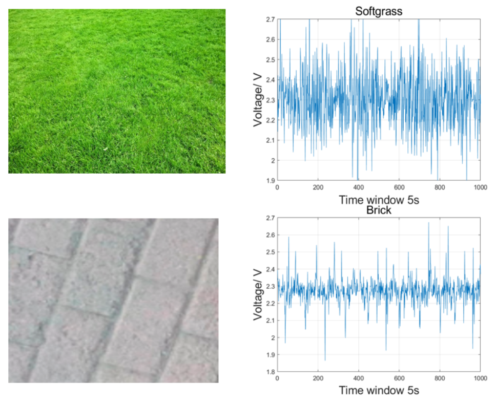
Based on the above methods, the whiskered robot was controlled by a Raspberry Pi 4 system to move on 7 different terrain surfaces: brick, cement, flat terrain, carpet, soft-grass, sand and a soft-soil surface respectively. All raw collected-data are pre-processed and the deep multi-layer perceptron neural network is pre-trained offline properly. Part of the sample experiment terrain surface and its corresponding vibration data are given in Figure 8.
This experiment collects 5 minutes of vibration data for each terrain surface. By randomly extracting 75 % data from the terrain tactile vibration database as the training data, and the rest 25% of data were used to test the performance of this network. The experimental parameters are set as shown in Table I. In all, 20 random experiments were conducted to avoid accidental errors caused by random trials.
| Parameters | Value | |
|---|---|---|
| Robot Velocity | 0.2 m/s | |
| Sampling Frequency | 200 Hz | |
| Time-window | 1 sec |

As can be seen from the Figure 9, the predicted classification success rates for flat terrain, carpet, cement, soft-grass, brick, sand and softsoil terrain surface are , , , , , 86.6%, and 85.8% respectively. The experimental results indicate that the whiskered tactile sensor and the deep multi-layer perception neural network have good recognition and identification capabilities of different terrains, with an average success rate of about 85.6%.The results shows that the steady state response of nonlinear vibration dynamics of whisker sensor can be used to classify different terrains.

Based on the confusion matrix in Figure 10, this network has high identification and classification success rate for flat and soft grass terrain surface because they have distinct vibration features based on their vibration signals. However, there is a high confusion rate between the flat surface and the brick surface which can be explained by the similar gap between the two adjacent units. In the case of the cement terrain, this could have a complicated surface including features such as gaps, a smooth or rugged surface which make the network more challenging to classify it from others.
Combined with the simulation results in Section III, the results indicate that robot’s base excitation vibration amplitude (i.e. ground profile height) affects the sensitivity of whisker sensor , and the sensor signal can provide enough information for classifying the sensor base excitation (terrain profile) by employing deep multi-layer perceptron neural network.
V-B Different Speed Experiments
The result of the previous section indicates that the whiskered tactile sensor and the proposed deep multi-layer perceptron neural network reported in this paper has good classification and identification capabilities on seven terrains at a constant velocity 0.2 m/s. The influence of different speeds on the sensor and model prediction accuracy has been analyzed. Data collection was performed at speeds of m/s, m/s, m/s, m/s and m/s respectively. All parameters during this experiment are the same as in the previous section. The identification accuracy results are shown in Table II.
| Speed | |||||||
| /s | |||||||
| 0.30m/s | 92.5% | 92.5% | 84.2% | 78.5% |
Looking at Figure 11 and Figure 12, it can be seen that this system has good identification accuracy for seven terrains surface at different speeds. The average prediction accuracy of the seven terrains at different speeds are: 83.31%, 85,74%, 85.60%, 87.8%, and 84.84%.


Therefore, speed has no consistent effect on identification success rate. However, there are still some details here that can be used as a reference to improve the identification accuracy. Firstly, the average identification accuracy at a speed of v = 0.25 m/s is higher than the other four operating states reaching 87.8%, which indicates that the speed of mobile robot has influence on identification accuracy. This may be caused by the dynamic resonance of the nonlinear experiment system. The spring beam and the robots car achieve a better resonance effect at m/s, which makes the spring vibration more obvious. Since the sensitivity of the sensor depends on the vibration of the spring, it has a better classification effect at this speed. This also echoes the simulation results of the Section III, indicating that robot’s base excitation vibration frequency affects the whisker tactile sensor sensitivity. Moreover, a nonlinear system has multiple resonance frequencies, this can also explain why good results are also achieved at the speed 0.15m/s but relatively poor at 0.2m/s.
Secondly, the accuracy of distinguishing between the brick and flat terrain surfaces increases when the robot speed increases. Combined with modal analysis in Section III, these results indicate that terrain surface profile amplitude and robots vibration frequency affects the sensor sensitivity in the same way. But, the surface amplitude is the dominant factor in affecting the sensor displacement for low frequency profile.
VI CONCLUSIONS
Whiskers, vestibular system, and the cochlear are three examples of compliant mechanical systems in biological counterparts that solve realtime perception problems using nonlinear vibration dynamics. Work done on such reservoir computing systems show that even periodic sinusoidal external perturbations can lead to complex steady state dynamics in the compliant mechanical system including period bifurcation and frequency separation at local sites. This paper shows for the first time that the steady state response of nonlinear vibration dynamics can be used to classify textures even on flat terrain. We also show that a mobile robot can use speed control to move the perturbation frequencies to elicit unique frequency domain responses in a whisker to help terrain classification. Experiment results show that the novel whiskered sensor and the deep multi-layer perceptron neural network have good recognition and identification capabilities of different terrain surfaces for mobile robots.
In the future, it will be interesting to investigate how realtime stiffness control of the whisker can be used as a control parameter to elicit steady state vibration frequency components unique to the texture and low frequency geometric features of a given terrain.
References
- [1] R. Siegwart, I. R. Nourbakhsh, and D. Scaramuzza, Introduction to autonomous mobile robots. MIT press, 2011.
- [2] A. Howard and H. Seraji, “Vision-based terrain characterization and traversability assessment,” Journal of Robotic Systems, vol. 18, no. 10, pp. 577–587, 2001.
- [3] B. Suger, B. Steder, and W. Burgard, “Traversability analysis for mobile robots in outdoor environments: A semi-supervised learning approach based on 3d-lidar data,” in 2015 IEEE International Conference on Robotics and Automation (ICRA). IEEE, 2015, pp. 3941–3946.
- [4] A. Valada and W. Burgard, “Deep spatiotemporal models for robust proprioceptive terrain classification,” The International Journal of Robotics Research, vol. 36, no. 13-14, pp. 1521–1539, 2017.
- [5] F. G. Oliveira, E. R. Santos, A. A. Neto, M. F. Campos, and D. G. Macharet, “Speed-invariant terrain roughness classification and control based on inertial sensors,” in 2017 Latin American Robotics Symposium (LARS) and 2017 Brazilian Symposium on Robotics (SBR). IEEE, 2017, pp. 1–6.
- [6] M. Fend, S. Bovet, H. Yokoi, and R. Pfeifer, “An active artificial whisker array for texture discrimination,” in Proceedings 2003 IEEE/RSJ International Conference on Intelligent Robots and Systems (IROS 2003)(Cat. No. 03CH37453), vol. 2. IEEE, 2003, pp. 1044–1049.
- [7] L. A. Huet, J. W. Rudnicki, and M. J. Hartmann, “Tactile sensing with whiskers of various shapes: determining the three-dimensional location of object contact based on mechanical signals at the whisker base,” Soft robotics, vol. 4, no. 2, pp. 88–102, 2017.
- [8] M. Salman and M. J. Pearson, “Advancing whisker based navigation through the implementation of bio-inspired whisking strategies,” in 2016 IEEE International Conference on Robotics and Biomimetics (ROBIO). IEEE, 2016, pp. 767–773.
- [9] T. J. Prescott, M. J. Pearson, B. Mitchinson, J. C. W. Sullivan, and A. G. Pipe, “Whisking with robots,” IEEE robotics & automation magazine, vol. 16, no. 3, pp. 42–50, 2009.
- [10] M. Fend, S. Bovet, and V. Hafner, “The artificial mouse-a robot with whiskers and vision,” in Proceedings of the 35th International Symposium on Robotics (ISR 2004). Citeseer, 2004.
- [11] M. Salman and M. J. Pearson, “Whisker-ratslam applied to 6d object identification and spatial localisation,” in Conference on Biomimetic and Biohybrid Systems. Springer, 2018, pp. 403–414.
- [12] M. Brecht, B. Preilowski, and M. M. Merzenich, “Functional architecture of the mystacial vibrissae,” Behavioural brain research, vol. 84, no. 1-2, pp. 81–97, 1997.
- [13] M. J. Pearson and M. Salman, “Active whisker placement and exploration for rapid object recognition,” in 2019 IEEE/RSJ International Conference on Intelligent Robots and Systems (IROS). IEEE, 2019, pp. 672–677.
- [14] M. Kaneko, N. Kanayama, and T. Tsuji, “Active antenna for contact sensing,” IEEE Transactions on robotics and automation, vol. 14, no. 2, pp. 278–291, 1998.
- [15] D. B. Zurek and C. Gilbert, “Static antennae act as locomotory guides that compensate for visual motion blur in a diurnal, keen-eyed predator,” Proceedings of the Royal Society B: Biological Sciences, vol. 281, no. 1779, p. 20133072, 2014.
- [16] J. H. Solomon and M. J. Hartmann, “Extracting object contours with the sweep of a robotic whisker using torque information,” The International Journal of Robotics Research, vol. 29, no. 9, pp. 1233–1245, 2010.
- [17] H. Wegiriya, N. Herzig, S.-A. Abad, S. H. Sadati, and T. Nanayakkara, “A stiffness controllable multimodal whisker sensor follicle for texture comparison,” IEEE Sensors Journal, vol. 20, no. 5, pp. 2320–2328, 2019.
- [18] K. Nakajima, “Physical reservoir computing—an introductory perspective,” Japanese Journal of Applied Physics, vol. 59, no. 6, p. 060501, 2020.
- [19] K. Nakajima, H. Hauser, T. Li, and R. Pfeifer, “Information processing via physical soft body,” Scientific reports, vol. 5, no. 1, pp. 1–11, 2015.
- [20] J. Tao and H. Cheng, “Dynamic stress response and fatigue life of cantilever beam under non-Gaussian base excitation,” 2014, iSSN: 1392-8716 Issue: 3 Number: 3 Pages: 1284-1296 Publisher: JVE International Ltd. Volume: 16. [Online]. Available: https://www.jvejournals.com/article/15032