André F. T. Martins, Marcos Treviso, António Farinhas, Pedro M. Q. Aguiar, Mário A. T. Figueiredo, Mathieu Blondel, and Vlad Niculae

Sparse Continuous Distributions and Fenchel-Young Losses

André F. T. Martins andre.t.martins@tecnico.ulisboa.pt Affiliation: Instituto de Telecomunicações, Instituto Superior Técnico Affiliation: Lisbon ELLIS Unit (LUMLIS) & Unbabel, Lisbon, Portugal Marcos Treviso marcos.treviso@tecnico.ulisboa.pt Affiliation: Instituto de Telecomunicações, Instituto Superior Técnico, Lisbon, Portugal António Farinhas antonio.farinhas@tecnico.ulisboa.pt Affiliation: Instituto de Telecomunicações, Instituto Superior Técnico, Lisbon, Portugal Pedro M. Q. Aguiar aguiar@isr.ist.utl.pt Affiliation: Instituto de Sistemas e Robótica, Instituto Superior Técnico Affiliation: Lisbon ELLIS Unit (LUMLIS), Lisbon, Portugal Mário A. T. Figueiredo mario.figueiredo@tecnico.ulisboa.pt Affiliation: Instituto de Telecomunicações, Instituto Superior Técnico Affiliation: Lisbon ELLIS Unit (LUMLIS), Lisbon, Portugal Mathieu Blondel mblondel@google.com Affiliation: Google Research, Paris, France Vlad Niculae v.niculae@uva.nl Affiliation: Language Technology Lab, University of Amsterdam, The Netherlands

Abstract

Exponential families are widely used in machine learning, including many distributions in continuous and discrete domains (e.g., Gaussian, Dirichlet, Poisson, and categorical distributions via the softmax transformation). Distributions in each of these families have fixed support. In contrast, for finite domains, recent work on sparse alternatives to softmax (e.g., sparsemax, $\alpha$ -entmax, and fusedmax), has led to distributions with varying support.

This paper develops sparse alternatives to continuous distributions, based on several technical contributions: First, we define $\Omega$ -regularized prediction maps and Fenchel-Young losses for arbitrary domains (possibly countably infinite or continuous). For linearly parametrized families, we show that minimization of Fenchel-Young losses is equivalent to moment matching of the statistics, generalizing a fundamental property of exponential families. When $\Omega$ is a Tsallis negentropy with parameter $\alpha$ , we obtain “deformed exponential families,” which include $\alpha$ -entmax and sparsemax ( $\alpha=2$ ) as particular cases. For quadratic energy functions, the resulting densities are $\beta$ -Gaussians, an instance of elliptical distributions that contain as particular cases the Gaussian, biweight, triweight, and Epanechnikov densities, and for which we derive closed-form expressions for the variance, Tsallis entropy, and Fenchel-Young loss. When $\Omega$ is a total variation or Sobolev regularizer, we obtain a continuous version of the fusedmax. Finally, we introduce continuous-domain attention mechanisms, deriving efficient gradient backpropagation algorithms for $\alpha\in\{1,\nicefrac{{4}}{{3}},\nicefrac{{3}}{{2}},2\}$ . Using these algorithms, we demonstrate our sparse continuous distributions for attention-based audio classification and visual question answering, showing that they allow attending to time intervals and compact regions.

^†^†shortheadings: Sparse Continuous Distributions and Fenchel-Young Losses / Sparse Continuous Distributions and Fenchel-Young Losses^†^†firstpage: 1^†^†heading: 23 2022 1- 8/21; Revised 4/22 7/22 21-0879^†^†shortheadings: Sparse Continuous Distributions and Fenchel-Young Losses / Martins, Treviso, Farinhas, Aguiar, Figueiredo, Blondel, and Niculae^†^†editor: Sebastian Nowozin

keywords

Sparse continuous distributions, Fenchel-Young losses, deformed exponential families, attention mechanisms.

1 Introduction

Exponential families (Brown 1986; Barndorff-Nielsen 2014) are ubiquitous in statistics and machine learning. They include many common distributions, both in continuous (Gaussian, exponential, Dirichlet, …) and discrete (Poisson, Bernoulli, categorical, …) domains. They enjoy many useful properties, such as the existence of conjugate priors (crucial in Bayesian inference) and the classical Pitman-Koopman-Darmois theorem (Pitman 1936; Darmois 1935; Koopman 1936), which states that, among families with fixed support (independent of the parameters), exponential families are the only having sufficient statistics of fixed dimension for any number of i.i.d. samples.

There have been several efforts to further generalize exponential families. Grünwald and Dawid 2004 introduced generalized exponential families as maximum entropy distributions for generalized entropy functions. Based upon these results, Frongillo and Reid 2014 studied these distributions from a convex duality perspective. Amari et al. 2012 studied deformed exponential families, including their entropy and canonical divergence.

More recently, there has been work with a focus on distributions with varying and sparse support over a finite domain. Examples include sparsemax (Martins and Astudillo 2016), entmax (Peters et al. 2019; Correia et al. 2019), and fusedmax (Niculae and Blondel 2017). They have been used for sparse differentiable dynamic programming (Mensch and Blondel 2018) and for improving the interpretability of attention mechanisms in neural networks (Bahdanau et al. 2015).

A common task when it comes to probability distributions is to fit their parameters to observed data. Unfortunately, unlike for exponential families, maximum likelihood for generalized exponential families does not always lead to a convex objective with respect to the parameters. Proper scoring rules, which can be seen as primal-space Bregman divergences, have been widely studied (Gneiting and Raftery 2007; Reid and Williamson 2010; Williamson et al. 2016). Typically, proper scoring rules are composed with a link function. However, when the link function is non-invertible, which is the case with sparse distributions, the resulting composite loss function can be non-convex (Blondel et al. 2020). Based on convex duality arguments, Blondel et al. 2020 introduced Fenchel-Young losses, which can be seen as mixed-space Bregman divergences (Amari 2016, Theorem 1.1). Unlike with proper scoring rules, the link function, called regularized prediction map, is not explicitly composed with the loss but instead kept implicit. This leads to convex loss functions, even for distributions with sparse support.

This paper.

We extend sparse probability distributions and Fenchel-Young losses to infinite domains (continuous or countably infinite). Similarly to (and generalizing) the free energy variational principle (Dayan et al. 1995), a convex regularizer $\Omega$ , which can be regarded as a generalized negentropy, induces a mapping from energy functions to probability densities. When $\Omega$ is a Tsallis negentropy (Tsallis 1988), the resulting densities are deformed exponential families. These families have been studied in statistical physics and machine learning (Naudts 2009; Sears 2008; Ding and Vishwanathan 2010) with most focus given to heavy-tailed distributions. Our paper focuses instead on light and zero-tailed distributions, which can be regarded as continuous counterparts of sparsemax and entmax transformations. We use this construction to obtain new density families, called $\alpha$ -sparse families, with sparse and varying support, including the truncated parabola/paraboloid distributions and the wider family of $\beta$ -Gaussian distributions (see Figures 4 and 7). In addition, we also provide a continuous counterpart for the discrete smoothing fusedmax transformation (Niculae and Blondel 2017) by designing a $\Omega$ that depends on the density derivative, via Rudin-Osher-Fatemi and Sobolev regularization (Rudin et al. 1992).

We use our theoretical results above in two ways. First, we extend neural attention mechanisms (Bahdanau et al. 2015) to continuous domains, making them able to attend to continuous data streams and to domains that are inherently continuous, such as visual scenes. Unlike traditional attention mechanisms, ours are suitable for selecting compact regions, such as 1D-segments or 2D-ellipses, and we illustrate this fact on audio classification and visual question answering tasks. Second, we demonstrate the usefulness of continuous-domain Fenchel-Young losses in a simple heteroscedastic regression problem modeled with bounded noise (d’Onofrio 2013).

To encourage reproducibility and further experimentation by the research community, we release an easy-to-use Python package alongside our paper: https://github.com/deep-spin/sparse_continuous_distributions/.

Previous papers.

This paper builds upon two previously published papers: a journal paper (Blondel et al. 2020) and a shorter conference paper (Martins et al. 2020). The former introduced and analyzed Fenchel-Young losses for finite and combinatorial domains, with a focus on structured prediction, without considering non-finite probability spaces. The latter focused on regularized prediction maps with Tsallis regularizers and sparse and continuous attention mechanisms, but without considering Fenchel-Young losses. This paper provides a comprehensive study of regularized prediction maps and Fenchel-Young losses for arbitrary measure spaces, including continuous and countably infinite domains, being a natural companion for Blondel et al. 2020. Besides a much more thorough treatment of previously covered topics, this paper contributes entirely new sections, including §3 on Fenchel-Young losses for arbitrary measure spaces and parametrized families, §6 on elliptical distributions and $\beta$ -Gaussians, and §7 on a continuous generalization of fusedmax. We also provide additional properties of Tsallis regularized families in §4 (Propositions 10 and 11) and more examples of sparse families in §5, such as the sparse Poisson and the truncated Gaussian. We derive closed form expressions for Fenchel-Young losses with several continuous densities (including $\beta$ -Gaussians, in Proposition 18) and demonstrate how to use our framework to fit continuous densities on data by Fenchel-Young loss minimization, not covered in the previous two papers.

Notation.

Let $(S,\mathcal{A},\nu)$ be a measure space, where $S$ is a set, $\mathcal{A}$ is a $\sigma$ -algebra, and $\nu$ is a measure. We denote by $\mathcal{M}_{+}^{1}(S)$ the set of $\nu$ -absolutely continuous probability measures. From the Radon-Nikodym theorem (Halmos 2013, §31), each element of $\mathcal{M}_{+}^{1}(S)$ is identified (up to equivalence within measure zero) with a probability density function $p:S\rightarrow\mathbb{R}_{+}$ , with $\int_{S}p(t)\,d\nu(t)=1$ . For convenience, we often drop $d\nu(t)$ from the integral. We denote the measure of $A\in\mathcal{A}$ as $|A|=\nu(A)=\int_{A}1$ , and the support of a density $p\in\mathcal{M}_{+}^{1}(S)$ as $\mathrm{supp}(p)=\{t\in S\mid p(t)>0\}$ . Given $\phi:S\rightarrow\mathbb{R}^{m}$ , we write expectations as $\mathbb{E}_{p}[\phi(t)]:=\int_{S}p(t)\,\phi(t)$ . Finally, we define $[a]_{+}:=\max\{a,0\}$ .

Throughout the paper, we use the following definition of ‘‘sparse densities’’,¹¹ 1 This should not be confused with sparsity-inducing distributions (Figueiredo 2001; Tipping 2001). which generalizes the notion of sparse vectors, recovered when $S$ is finite and $\nu$ is the counting measure. The concept is illustrated in Figure 1.

Definition 1 (Sparse density.).

Let $(S,\mathcal{A},\nu)$ be a measure space. A density $p:S\rightarrow\mathbb{R}$ is called sparse if $\nu(S\setminus\mathrm{supp}(p))>0$ . It is called dense otherwise.

Figure 1: Non-sparse and sparse densities for

S=\mathbb{R}

. Left: The density

p(t)=\sin^{2}(t)/(\pi t^{2})

is non-sparse, since it has only a countable number of zeros and therefore the set

\mathbb{R}\setminus\mathrm{supp}(p)

has null measure. Right: Univariate

\beta

-Gaussians

\mathcal{N}_{\beta}(t,0,\sigma^{2})

for several values of

\alpha=2-\beta

(see §6 for details). We used

\sigma^{2}=1

except for

\alpha=0

, for which

\sigma^{2}=(2\pi)^{-1}

(Cauchy distribution).

\alpha=1

corresponds to a Gaussian,

\alpha<1

to heavy-tail distributions (

t

-Student), and

\alpha>1

to zero-tail distributions, recovering scaled versions of the biweight (

\alpha=\tfrac{3}{2}

), triweight (

\alpha=\tfrac{4}{3}

), and Epanechnikov kernels (

\alpha=2

, same as truncated parabola) used in density estimation. For

\alpha>1

, the case of focus in our paper, all these densities are sparse.

Table of contents.

The rest of the paper is organized as follows. Figure 2 helps navigating through the different sections.

§2

Regularized Prediction Maps
§3

Continuous Fenchel-Young Losses
§4

Tsallis Regularizers and Deformed Exponential Families
§5

Infinite Sparsemax
§6

Elliptical Distributions and $\beta$ -Gaussians
§7

Continuous Fusedmax
§8

Continuous Attention Mechanisms
§9

Experiments
§10

Related work.

Figure 2: Diagram representing

\Omega

-regularized prediction maps (§2–§3) and some of its particular cases covered in this paper.

\beta

-Gaussian distributions (§6) lie at the intersection of elliptical distributions and deformed exponential families, corresponding to quadratic energies, and they include the Gaussian and Truncated Paraboloid (TP) distributions as particular cases. Exponential families and (infinite) sparsemax distributions (§5) are a particular case of deformed exponential families (§4) for

\alpha\in\{1,2\}

; examples of such distributions for different energy functions are given in Table 1. Fusedmax distributions (§7) extend 1-d sparsemax by incorporating total variation or Sobolev regularizers.

2 Regularized Prediction Maps

The crux of this paper is the notion of $\Omega$ -regularized prediction maps, which have been introduced by Blondel et al. 2020 for finite domains $S$ , and which we generalize here to arbitrary measure spaces. We will show in the sequel that these maps generalize the free energy variational principle (Dayan et al. 1995).

2.1 Warm-up: Finite domains

Let us start with the finite case, $S=[K]=\{1,\ldots,K\}$ . We consider the following problem: given a vector of real numbers $f\in\mathbb{R}^{K}$ , convert them into a probability vector $p\in\triangle^{K}$ , where $\triangle^{K}:=\{p\in\mathbb{R}^{K}\mid p\geq 0,\,\,p^{\top}1=1\}$ denotes the probability simplex. For example, $f$ could be a vector of label scores (or “logits”) computed by a neural network classifier, and $p$ the corresponding label probabilities. The idea behind regularized prediction maps is to smooth the argmax operator with a convex regularizer $\Omega:\triangle^{|S|}\rightarrow\mathbb{R}$ which encourages uniform distributions:

\hat{p}_{\Omega}[f]=\argmax_{p\in\triangle^{|S|}}p^{\top}f-\Omega(p).

(1)

This operator can be regarded as the gradient map of the smoothed max function $\max_{\Omega}(f):=\max_{p\in\triangle^{|S|}}p^{\top}f-\Omega(p)$ (Nesterov 2005; Beck and Teboulle 2012; Niculae and Blondel 2017). Without any regularization ( $\Omega\equiv 0$ ), we obtain the argmax transformation, where the maximizer $p^{\star}$ in (1) becomes a one-hot vector. Non-trivial choices of $\Omega$ recover well-known transformations such as softmax (Bridle 1990), and recently proposed ones, including sparsemax (Martins and Astudillo 2016), fusedmax (Niculae and Blondel 2017), and entmax (Peters et al. 2019). We will cover these transformations in this paper and we will show in the subsequent sections how they can be extended to arbitrary infinite measure spaces (countably infinite or continuous).

2.2 Extension to infinite domains

In several practical applications, the domain $S$ is not finite: For example, it can be a continuous space, such as $\mathbb{R}$ or $\mathbb{R}^{N}$ , or a countably infinite set such as $\mathbb{N}$ . To accommodate this in an unified manner, we need to consider the space of probability densities $\mathcal{M}_{+}^{1}(S)$ instead of the probability simplex $\triangle^{|S|}$ . Our definition below extends regularized prediction maps to arbitrary measure spaces $S$ . Instead of a finite vector $f\in\mathbb{R}^{K}$ , we assume now a scoring function $f:S\rightarrow\mathbb{R}$ .

Definition 2 ( $\Omega$ -regularized prediction map.).

Let $\Omega:\mathcal{M}_{+}^{1}(S)\rightarrow\mathbb{R}$ be a lower semi-continuous (l.s.c.), proper, and strictly convex function. The $\Omega$ -regularized prediction map $\hat{p}_{\Omega}:\mathcal{F}\rightarrow\mathcal{M}_{+}^{1}(S)$ is defined as

\hat{p}_{\Omega}[f]=\argmax_{p\in\mathcal{M}_{+}^{1}(S)}\mathbb{E}_{p}[f(t)]-\Omega(p)=\argmax_{p\in\mathcal{M}_{+}^{1}(S)}\int_{S}p(t)\,f(t)\,d\nu(t)-\Omega(p),

(2)

where $\mathcal{F}$ is the set of functions for which the maximizer above exists and is unique.

Figure 3: Discrete and continuous

\Omega

-regularized prediction maps. For each case, we show the scoring function

f

(top) and corresponding distribution

\hat{p}_{\Omega}[f]

(bottom) when

\Omega

is the Shannon-Boltzmann-Gibbs entropy. Left: finite

S

. Right:

S=\mathbb{R}

Figure 3 provides an illustration.

Properties.

$\Omega$ -regularized prediction maps enjoy several important properties; see Blondel et al. 2020 for the finite $S$ case. For example, they are insensitive to the addition of constants, both to the regularizer $\Omega$ and to the function $f$ . That is, $\hat{p}_{\Omega}\equiv\hat{p}_{\Omega+c}$ for any $c\in\mathbb{R}$ and $\hat{p}_{\Omega}[f]=\hat{p}_{\Omega}[g]$ if $g(t)=f(t)+c$ . The former follows immediately from (2), and the latter follows from the fact that $\mathbb{E}_{p}[f(t)+c]=\mathbb{E}_{p}[f(t)]+c$ . For the continuous case $S=\mathbb{R}^{N}$ and if the regularizer $\Omega$ is separable (i.e. if it can be written as $\Omega(p)=\int_{S}\psi(p(t))$ for some function $\psi:\mathbb{R}_{+}\rightarrow\mathbb{R}$ ) – which is always the case in this paper – we also have the following equivariance property: if $\tilde{f}(t):=f(At+b)$ for a matrix $A$ with determinant $\pm 1$ , then $\hat{p}_{\Omega}[\tilde{f}](t)=\hat{p}_{\Omega}[f](At+b)$ . This includes equivariance with respect to translations and orthogonal transformations as particular cases. See Appendix A.1 for a proof.

Low temperature limit.

It is often convenient to consider a “temperature parameter” $\tau>0$ , absorbed into $\Omega$ via $\Omega:=\tau\tilde{\Omega}$ . If $f$ has a unique global maximizer $t^{\star}$ , the low-temperature limit yields ${\lim_{\tau\rightarrow 0}}\,\hat{p}_{\tau\tilde{\Omega}}[f]=\delta_{t^{\star}}$ , a Dirac delta distribution at the maximizer of $f$ . For finite $S$ , this is simply the argmax transformation. More interesting examples of regularization functionals are shown in the next sections.

2.3 Examples

Shannon-Boltzmann-Gibbs entropy.

If we interpret $-f(t)$ as an energy function and choose as regularizer the Shannon-Boltzmann-Gibbs negentropy²² 2 This includes as particular cases the Shannon negentropy when $\nu$ is the counting measure for discrete $S$ , and the differential negentropy when $\nu$ is the Lebesgue measure for continuous $S$ . Shannon-Boltzmann-Gibbs negentropies are however more general and they can work with arbitrary measures. $\Omega(p)=\int_{S}p(t)\log p(t)d\nu(t)$ , we recover the well-known free energy variational principle (Dayan et al. 1995). In that case, the quantity $-U_{\Omega}(p;f):=-\mathbb{E}_{p}[f(t)]+\Omega(p)$ corresponds to the Helmholtz free energy, and $\hat{p}_{\Omega}$ is its minimizer (Hinton and Zemel 1993). With this choice, the solution of the optimization problem (2) is a Boltzmann-Gibbs distribution (Cover and Thomas 2012; see Appendix A.2 for a proof):

\hat{p}_{\Omega}[f](t)=\frac{\exp(f(t))}{\int_{S}\exp(f(t^{\prime}))d\nu(t^{\prime})}=\exp\bigl(f(t)-A(f)\bigr),

(3)

where $A(f):=\log\int_{S}\exp(f(t))$ is the log-partition function. Some particular cases are:

•

If $S$ is finite and $\nu$ is the counting measure, the integral in (3) is a summation and we can write $f$ as a vector $[f_{1},\ldots,f_{|S|}]\in\mathbb{R}^{|S|}$ . In this case, the $\Omega$ -regularized prediction map is the softmax transformation,

$\hat{p}_{\Omega}[f]=\mathrm{softmax}(f)=\tfrac{\exp(f)}{\sum_{k=1}^{|S|}\exp(f_{k})}\in\triangle^{|S|}.$ (4)

The vector $\hat{p}_{\Omega}[f]$ parameterizes a categorical distribution in this case.
•

If $S=\mathbb{N}$ , $\nu(A)$ the counting measure, and $f(t)=t\log\lambda-\log(t!)$ for $\lambda>0$ , we obtain a Poisson distribution, $\mathrm{Pr}\{t=k\}=\frac{\hat{p}_{\Omega}[f](k)}{k!}=\frac{\lambda^{k}\exp(-\lambda)}{k!}$ , with $\Omega(\hat{p}_{\Omega}[f])=-\lambda(1-\log\lambda)-\exp(-\lambda)\sum_{t=0}^{\infty}\frac{\lambda^{t}\log(t!)}{t!}$ .³³ 3 It is also possible to obtain a Poisson distribution by letting $\nu(A)=\sum_{t\in A}\frac{1}{t!}$ for $A\subseteq\mathbb{N}$ , $f(t)=t\log\lambda$ for $\lambda>0$ , and $\Omega(p)=\sum_{k=0}^{\infty}\frac{p(k)\log p(k)}{k!}$ . The formulation above, however, is more convenient for sparse generalizations, as we shall see.
•

If $S=\mathbb{R}^{N}$ , $\nu$ is the Lebesgue measure, and $f(t)=-\frac{1}{2}(t-\mu)^{\top}\Sigma^{-1}(t-\mu)$ for $\mu\in\mathbb{R}^{N}$ and $\Sigma\succ 0$ , we obtain a multivariate Gaussian, $\hat{p}_{\Omega}[f](t)=\mathcal{N}(t;\mu,\Sigma)=(2\pi)^{-\nicefrac{{N}}{{2}}}|\Sigma|^{-\nicefrac{{1}}{{2}}}\exp(-\frac{1}{2}(t-\mu)^{\top}\Sigma^{-1}(t-\mu))$ , with differential negentropy $\Omega(\hat{p}_{\Omega}[f])=-\frac{1}{2}\log\det(2\pi e\Sigma)$ . This becomes a univariate Gaussian $\mathcal{N}(t;\mu,\sigma^{2})$ if $N=1$ .
•

For $S=\mathbb{R}$ and defining $f(t)=-|t-\mu|/b$ for $\mu\in\mathbb{R}$ and $b>0$ we get a Laplace density, $\hat{p}_{\Omega}[f](t)=\tfrac{1}{2b}\exp\left(-|t-\mu|/b\right)$ , with differential negentropy $\Omega(\hat{p}_{\Omega}[f])=-\log(2be)$ .

These distributions are summarized in Table 1 (rows with $\alpha=1)$ .

Sparsity-inducing regularizers.

Other regularizers $\Omega$ have been considered for the finite case. Choosing the Gini entropy $\Omega(p)=\tfrac{1}{2}\|p\|_{2}^{2}-\frac{1}{2}$ (equivalent to $\ell_{2}$ -regularization) leads to the sparsemax transformation (Martins and Astudillo 2016), and Tsallis entropy regularizers lead to entmax (Peters et al. 2019), covered later in this paper. These regularizers are able to promote sparse probability mass functions. However, their development has been limited so far to finite domains. In this paper, we generalize sparsemax and entmax to continuous domains (§4–§5). For entmax, we draw a new connection with elliptical distributions (Fang et al. 1990) when $f(t)$ is a quadratic scoring function (§6). In this case, the $\Omega$ -regularized prediction map leads to a generalization of multivariate Gaussian distributions called $\beta$ -Gaussians, which can have bounded support and relate to some well-known density estimation kernels (Epanechnikov 1969; Silverman 1986).

Table 1: Distributions induced by

\Omega_{\alpha}

-regularized prediction maps for several scoring functions

f

for finite, countably infinite, and continuous domains. We show the cases

\alpha\in\{1,2\}

(

\alpha=1

corresponds to the Shannon-Boltzmann-Gibbs regularizer, covered in §2.3, whereas

\alpha=2

corresponds to the Gini regularizer, covered in §5). We denote by

\|t-\mu\|^{2}_{\Sigma^{-1}}\!:=\!(t\!-\!\mu)^{\top}\Sigma^{-1}(t\!-\!\mu)

the squared Mahalanobis distance between

t

and

\mu

. The sparse Poisson and truncated paraboloid are new distributions presented in a unified manner with this framework.

Name	$S$	$f(t)$	$\alpha$	$\hat{p}_{\Omega_{\alpha}}[f]$	$\Omega_{\alpha}(\hat{p}_{\Omega_{\alpha}}[f])$
Categorical (softmax)	$[K]$	$f_{t}$	$1$	$\tfrac{\exp(f)}{\sum_{t=1}^{K}\exp(f_{t})}$	$\sum_{t=1}^{K}p_{t}\log p_{t}$
Sparsemax	$[K]$	$f_{t}$	$2$	$[f_{t}-\tau]_{+}$	$\frac{1}{2}\left(\sum_{t=1}^{K}p_{t}^{2}-1\right)$
Poisson	$\mathbb{N}$	$t\log\mu+\log(1/t!)$	$1$	$\mu^{t}\exp(-\mu)/t!$	$-\mu(1-\log\mu)-\exp(-\mu)\sum_{t=0}^{\infty}\frac{\mu^{t}\log(t!)}{t!}$
Sparse Poisson	$\mathbb{N}$	$t\log\mu+\log(1/t!)$	$2$	$[f(t)-\tau]_{+}$	$\frac{1}{2}\left(\sum_{t=0}^{\infty}[f(t)-\tau]_{+}^{2}-1\right)$
Gaussian	$\mathbb{R}$	$-\frac{(t-\mu)^{2}}{2\sigma^{2}}$	$1$	$\mathcal{N}(t;\mu,\sigma^{2})$	$-\nicefrac{{1}}{{2}}\log(2\pi e\sigma^{2})$
Truncated Parabola	$\mathbb{R}$	$-\frac{(t-\mu)^{2}}{2\sigma^{2}}$	$2$	$\left[f(t)-\tau\right]_{+}$	$-\frac{1}{2}+\frac{1}{5}\left(\frac{3}{2\sigma}\right)^{2/3}$
Laplace	$\mathbb{R}$	$-\frac{\|t-\mu\|}{b}$	$1$	$\frac{1}{2b}\exp\left(-\frac{\|t-\mu\|}{b}\right)$	$-\log(2be)$
Triangular	$\mathbb{R}$	$-\frac{\|t-\mu\|}{b}$	$2$	$\left[f(t)-\tau\right]_{+}$	$-\frac{1}{2}+\frac{1}{3\sqrt{b}}$
Multivariate Gaussian	$\mathbb{R}^{N}$	$-\frac{1}{2}\\|t-\mu\\|^{2}_{\Sigma^{-1}}$	$1$	$\mathcal{N}(t;\mu,\Sigma)$	$-\nicefrac{{1}}{{2}}\log\det(2\pi e\Sigma)$
Truncated Paraboloid	$\mathbb{R}^{N}$	$-\frac{1}{2}\\|t-\mu\\|^{2}_{\Sigma^{-1}}$	$2$	$[f(t)-\tau]_{+}$	$-\tfrac{1}{2}+\tfrac{2}{N+4}\left(\frac{\Gamma\left(\tfrac{N}{2}+2\right)}{(2\pi)^{\frac{N}{2}}\|\Sigma\|^{\frac{1}{2}}}\right)^{\tfrac{2}{2+N}}$

Table 2: Linear parametrization

f_{\theta}(t)=\theta^{\top}\phi(t)

for the scoring function

f(t)

of common distributions. We further require

\mu>0

for the (sparse) Poisson distribution. For the Laplace and Triangular distributions, we assume the location

\mu

known (fixed). As is standard, for Gaussians,

f(t)

is only linear in

\theta

up to a constant. In §6, we use the quadratic form directly.

Sparsemax	$[K]$	$f_{t}$	$[f_{1},\dots,f_{K}]$	$e_{t}$
Distribution	$S$	$f(t)$	$\theta$	$\phi(t)$
Categorical	$[K]$	$f_{t}$	$[f_{1},\dots,f_{K}]$	$e_{t}$
Poisson, Sparse Poisson	$\mathbb{N}$	$t\log\mu+\log(1/t!)$	$[\log\mu,1]$	$[t,\log(1/t!)]$
Gaussian	$\mathbb{R}$	$-\frac{(t-\mu)^{2}}{2\sigma^{2}}$	$[\frac{\mu}{\sigma^{2}},-\frac{1}{2\sigma^{2}}]$	$[t,t^{2}]$
Truncated Parabola	$\mathbb{R}$
Sparse Integer Gaussian	$\mathbb{Z}$
Laplace	$\mathbb{R}$	$-\frac{\|t-\mu\|}{b}$	$[-\frac{1}{b}]$	$[\|t-\mu\|]$
Triangular	$\mathbb{R}$	$-\frac{\|t-\mu\|}{b}$	$[-\frac{1}{b}]$	$[\|t-\mu\|]$
Multivariate Gaussian	$\mathbb{R}^{N}$	$-\frac{1}{2}\\|t-\mu\\|^{2}_{\Sigma^{-1}}$	$[\Sigma^{-1}\mu,-\frac{1}{2}\mathrm{vec}(\Sigma^{-1})]$	$[t,\mathrm{vec}(tt^{\top})]$
Truncated Paraboloid	$\mathbb{R}^{N}$	$-\frac{1}{2}\\|t-\mu\\|^{2}_{\Sigma^{-1}}$	$[\Sigma^{-1}\mu,-\frac{1}{2}\mathrm{vec}(\Sigma^{-1})]$	$[t,\mathrm{vec}(tt^{\top})]$

Total variation regularizer.

Also for the finite case, Niculae and Blondel 2017 proposed fusedmax, which corresponds to the regularizer $\Omega(p)=\tfrac{1}{2}\|p\|_{2}^{2}+\sum_{k=1}^{|S|-1}|p_{k+1}-p_{k}|$ , inspired by the fused lasso (Tibshirani et al. 2005). Besides sparsity, this regularizer encourages the same probability value in contiguous elements. We generalize fusedmax to continuous domains in §7, by replacing the finite difference $|p_{k+1}-p_{k}|$ by the derivative $|p^{\prime}(t)|$ , leading to Rudin-Osher-Fatemi and Sobolev regularizers.

Linearly parametrized families of scoring functions.

Definition 2 is fully general concerning the class of functions $\mathcal{F}$ from which $f$ can be chosen. In practice, it is often useful to consider finite-dimensional parametrized function classes. The simplest way to do this is via linear functions $f_{\theta}(t)=\theta^{\top}\phi(t)$ , where $\phi(t)\in\mathbb{R}^{M}$ is a vector of statistics and $\theta\in\Theta\subseteq\mathbb{R}^{M}$ is a vector of canonical parameters.⁴⁴ 4 More generally, we can write $f_{\theta}(t)=\theta^{\top}\phi(t)+c(\theta)+d(t)$ where $c$ and $d$ are functions. However, these extra terms can also be handled by absorbing $c(\theta)$ into the normalization constant or $d(t)$ into the base measure. A family of the form (3) parametrized by $\theta\in\Theta$ is called an exponential family (Barndorff-Nielsen 2014). All the examples above (the categorical distribution with the softmax transformation, the Poisson with parameter $\lambda$ , the Gaussian with parameters $\mu$ and $\Sigma$ , and the Laplace with fixed $\mu$ and parameter $b$ ) are instances of exponential families. Exponential families have many appealing properties, such as the existence of conjugate priors and sufficient statistics, and a dually flat geometric structure (Amari 2016). A key property of exponential families is that the support is constant within the same family and dictated by the base measure $\nu$ : this follows immediately from the positiveness of the $\exp$ function in (3). In §4, we describe a more general set of families – deformed exponential families – that relax this property.

3 Continuous Fenchel-Young Losses

We saw in §2 how to construct distributions $\hat{p}_{\Omega}[f]$ from a scoring function $f(t)$ via the $\Omega$ -regularized prediction map (2). In practice, the scoring function will often be a parametrized function, denoted $f_{\theta}(t)$ . In this section, we will address the reverse problem: given a true data distribution $p$ (or samples thereof), find an estimate $\theta$ such that $\hat{p}_{\Omega}[f_{\theta}]\approx p$ . Many statistical tasks can be formulated in terms of finding a good empirical approximation to $p$ , and loss functions are a flexible way of quantifying how good these approximations are. For finite $S$ , Blondel et al. 2020 introduced the notion of Fenchel-Young loss. Here, we extend that notion to arbitrary domains.

3.1 Definition

The construction hinges on the notion of Fenchel dual, denoted $\Omega^{*}$ , of an l.s.c. proper convex function $\Omega\!:\!\mathcal{M}_{+}^{1}(S)\rightarrow\mathbb{R}$ (Bauschke and Combettes 2011):⁵⁵ 5 Fenchel duality is taken in the (potentially infinite-dimensional) set $\mathcal{F}\subseteq\mathbb{R}^{S}$ , which endowed with the inner product $\langle f,g\rangle=\int_{S}f(t)g(t)d\nu(t)$ forms a Hilbert space (Bauschke and Combettes 2011).

\Omega^{*}(f):=\max_{p\in\mathcal{M}_{+}^{1}(S)}\mathbb{E}_{p}[f(t)]-\Omega({p})=\mathbb{E}_{\hat{p}_{\Omega}[f]}[f(t)]-\Omega(\hat{p}_{\Omega}[f]),

where, for the equality, we used the fact that $\hat{p}_{\Omega}[f]$ is the solution of (2). We can now define the Fenchel-Young loss for arbitrary domains.

Definition 3 (Fenchel-Young loss.).

Given an l.s.c., proper, strictly convex function $\Omega:\mathcal{M}_{+}^{1}(S)\rightarrow\mathbb{R}$ , the Fenchel-Young loss $L_{\Omega}:\mathcal{F}\times\mathcal{M}_{+}^{1}(S)\rightarrow\mathbb{R}$ is defined as

L_{\Omega}(f;p):=\Omega^{*}(f)+\Omega(p)-\mathbb{E}_{p}[f(t)].

(5)

For convenience, we also define the cross- $\Omega$ loss $L^{\times}_{\Omega}:\mathcal{F}\times\mathcal{M}_{+}^{1}(S)\rightarrow\mathbb{R}$ as follows:

L^{\times}_{\Omega}(f;p):=\Omega^{*}(f)-\mathbb{E}_{p}[f(t)].

(6)

Note that, when $\Omega(p)$ is finite, the Fenchel-Young loss $L_{\Omega}$ differs from $L^{\times}_{\Omega}$ only by a term which is constant w.r.t. $f$ . An interesting example is when $p=\delta_{t}$ is a Dirac delta, in which case we obtain $L^{\times}_{\Omega}(f;\delta_{t})=\Omega^{*}(f)-\mathbb{E}_{\delta_{t}}[f(t)]=\Omega^{*}(f)-f(t)$ .

The name “Fenchel-Young loss” stems from the Fenchel-Young inequality (Borwein and Lewis 2010, Proposition 3.3.4), which immediately implies the following property:

Proposition 4 (Non-negativity and condition for zero loss).

With $\Omega$ as in Definition 3, we have (i) $L_{\Omega}(f;p)\geq 0$ , and (ii) $L_{\Omega}(f;p)=0\Leftrightarrow p=\hat{p}_{\Omega}[f]$ almost everywhere.

In fact, we can interpret the Fenchel-Young loss as the regret associated to the generalized Helmholtz free energy $-U_{\Omega}(p;f):=-\mathbb{E}_{p}[f(t)]+\Omega(p)$ : indeed, we have $\Omega^{*}(f)=\max_{p^{\prime}\in\mathcal{M}_{+}^{1}(S)}U_{\Omega}(p^{\prime};f)=U_{\Omega}(\hat{p}_{\Omega}[f];f)$ , and therefore $L_{\Omega}(f;p)=-U_{\Omega}(p;f)+U_{\Omega}(\hat{p}_{\Omega}[f];f)$ .

Fenchel-Young losses are also tightly connected to Bregman divergences (Bregman 1967), as shown by Amari 2016 and Blondel et al. 2020. In particular, when $\Omega$ is the Shannon-Boltzmann-Gibbs negentropy, the Fenchel-Young loss $L_{\Omega}$ equals the Kullback-Leibler divergence between $p$ and $\hat{p}_{\Omega}[f]$ , and $L^{\times}_{\Omega}$ becomes the cross-entropy loss. This is commonly used as an objective to minimize in estimation problems, for example when $\bar{p}:=\frac{1}{L}\sum_{\ell=1}^{L}\delta_{t_{\ell}}$ is the empirical data distribution associated to a sample $\{t_{1},\ldots,t_{L}\}$ , and the goal is to obtain an estimate $f$ so that $\hat{p}_{\Omega}[f]$ approximates $\bar{p}$ . In that case, the minimization of the cross-entropy loss corresponds to maximum likelihood estimation.⁶⁶ 6 Note that, for finite $S$ , $\Omega(\delta_{t})=0$ and therefore $L_{\Omega}^{\times}(f,\delta_{t})=L_{\Omega}(f,\delta_{t})$ . This, however, does not happen in general – for $S=\mathbb{R}$ , the differential negentropy explodes for Dirac distributions, $\Omega(\delta_{t})=+\infty$ .

3.2 Properties

Proposition 4 shows that Fenchel-Young losses generalize a key property of the Kullback-Leibler divergence and the cross-entropy loss, since the loss minimizers are attained when $\hat{p}_{\Omega}[f]=p$ . Indeed, one target use of Fenchel-Young losses is to obtain an estimate $f$ , given some empirical data distribution $\bar{p}$ , by minimizing $L_{\Omega}(f;\bar{p})$ . To make this practical, we need to assume a parametric family $\{f_{\theta}\mid\theta\in\Theta\}\subseteq\mathcal{F}$ , where $\theta$ is a vector of parameters and $\Theta\subseteq\mathbb{R}^{M}$ is a convex set. The goal of estimation is to find $\hat{\theta}$ which minimizes $L_{\Omega}(f_{\theta};\bar{p})$ . The next proposition, proved in Appendix B, sheds light on this problem.

Proposition 5 (Stationary points of Fenchel-Young losses).

Assume that $f_{\theta}(t)$ is differentiable with respect to $\theta\in\Theta$ for any $t\in S$ . Then, the following expression holds for the gradient of $L_{\Omega}(f_{\theta};p)$ with respect to $\theta$ :

\nabla_{\theta}L_{\Omega}(f_{\theta};p)=\mathbb{E}_{\hat{p}_{\Omega}[f_{\theta}]}[\nabla_{\theta}f_{\theta}(t)]-\mathbb{E}_{p}[\nabla_{\theta}f_{\theta}(t)].

(7)

Therefore, $\hat{\theta}\in\Theta$ is a stationary point of $L_{\Omega}(f_{\theta};p)$ iff it satisfies the equation

\mathbb{E}_{\hat{p}_{\Omega}[f_{\hat{\theta}}]}[\nabla_{\theta}f_{\theta}(t)]=\mathbb{E}_{p}[\nabla_{\theta}f_{\theta}(t)].

(8)

Eqs. (7)–(8) resemble the familiar gradient expressions used to estimate energy-based models with maximum likelihood (LeCun et al. 2006). Indeed, these expressions are recovered when $\Omega$ is the Shannon-Boltzmann-Gibbs entropy, in which case the distribution ${\hat{p}_{\Omega}[f_{\theta}]}$ is a Gibbs distribution, as seen in §2. Therefore, Fenchel-Young losses offer a more general objective function to fit densities in energy-based models which can serve as an alternative to maximum likelihood.

Convexity, moment matching, and sufficient statistics.

If the parametric family is linear, $f_{\theta}(t)=\theta^{\top}\phi(t)$ , then the gradient of $f$ with respect to $\theta$ becomes simply $\nabla_{\theta}f_{\theta}(t)=\phi(t)$ , and we obtain the following stronger properties, also proved in Appendix B:

Proposition 6 (Properties when $f_{\theta}(t)$ is linear in $\theta$ ).

If $f_{\theta}(t)=\theta^{\top}\phi(t)$ , then the following holds:

1.

$\nabla_{\theta}L_{\Omega}(f_{\theta};p)=\mathbb{E}_{\hat{p}_{\Omega}[f_{\theta}]}[\phi(t)]-\mathbb{E}_{p}[\phi(t)]$ .
2.

$L_{\Omega}(f_{\theta};p)$ is convex w.r.t. $\theta$ .
3.

$\hat{\theta}\in\arg\min_{\theta}L_{\Omega}(f_{\theta};p)\Leftrightarrow\mathbb{E}_{\hat{p}_{\Omega}[f_{\hat{\theta}}]}[\phi(t)]=v$ , where $v=\mathbb{E}_{p}[\phi(t)]$ .

The third point in Proposition 6 is particularly significant: If $p=\bar{p}$ is an empirical data distribution based on a sample $\{t_{1},\ldots,t_{L}\}$ , then $v=\frac{1}{L}\sum_{\ell=1}^{L}\phi(t_{\ell})$ is the empirical mean of the statistics – the statement shows that estimating $\theta$ only depends on $\bar{p}$ through $v$ , which generalizes the concept of sufficient statistics from exponential families. The result shows that fitting a density from a linearly parametrized family to an empirical distribution $\bar{p}$ by matching the expected statistics is optimal in the Fenchel-Young loss sense, generalizing the well-known result from exponential families that maximum likelihood estimation is equivalent to moment matching of the sufficient statistics.

Figure 4 illustrates the result of fitting $\beta$ -Gaussian distributions (to be introduced in §5) to samples drawn from each of the distributions by minimizing the corresponding Fenchel-Young losses, confirming adequate fitting.

Figure 4: Density and samples of two-dimensional

\beta

-Gaussian random variables, for the isotropic (top) and anisotropic cases (bottom). These distributions are obtained by applying (Tsallis)

\Omega_{\alpha}

-regularized prediction maps to quadratic scoring functions, with

\alpha=2-\beta

. Shown are the original density (solid lines) and the density fit to samples by moment matching (dashed lines). All contour lines are at the same absolute levels, and the complement of the support is shaded when appropriate.

3.3 Examples

We next provide some familiar examples, which will be generalized in the upcoming sections.

Examples 1 and 2: Squared and absolute losses.

Let $\Omega$ be the Shannon-Boltzmann-Gibbs negentropy. Let $p=\delta_{t}$ , i.e., the distribution contains a single sample $t$ . For the Gaussian distribution, by identification with (3), we get $\Omega^{*}(f)=A(f)=\log(\sigma\sqrt{2\pi})$ and therefore

L^{\times}_{\Omega}(f;p)=\frac{(t-\mu)^{2}}{2\sigma^{2}}+\log(\sigma\sqrt{2\pi}).

(9)

Similarly, for the Laplace distribution, we get $\Omega^{*}(f)=A(f)=\log(2b)$ and therefore

L^{\times}_{\Omega}(f;p)=\frac{|t-\mu|}{b}+\log(2b).

(10)

Example 3: KL divergence between two Gaussian distributions.

When $\Omega$ is the Shannon-Boltzmann-Gibbs entropy, the Fenchel dual is the log-partition function (3), $\Omega^{*}(f)=A(f)$ , and the Fenchel-Young loss recovers the Kullback-Leibler divergence. For example, if $S=\mathbb{R}^{N}$ , $p(t)=\mathcal{N}(t;\mu,\Sigma)$ , and $f(t)=-\frac{1}{2}(t-\mu_{f})^{\top}\Sigma_{f}^{-1}(t-\mu_{f})$ , using the expression for the entropy in §2, we obtain the well-known expression for the Kullback-Leibler divergence between Gaussians:

L_{\Omega}(f;p)=\frac{1}{2}(\mu-\mu_{f})^{\top}\Sigma_{f}^{-1}(\mu-\mu_{f})+\frac{1}{2}\left(\mathrm{Tr}(\Sigma_{f}^{-1}\Sigma)-N+\log\frac{|\Sigma_{f}|}{|\Sigma|}\right).

(11)

In §6, we will generalize this result for a class of elliptical distributions called $\beta$ -Gaussian distributions, for which we will derive a closed-form expression for the Fenchel-Young loss.

4 Tsallis Regularizers and Deformed Exponential Families

We introduce in this section a broader set of regularizers $\Omega$ based on Tsallis entropies (Tsallis 1988), which allow generalizing the examples in §3.3. Tsallis entropies are a generalization of Shannon-Boltzmann-Gibbs entropies which are suitable to model several phenomena present in natural, artificial and social complex systems (Lutz 2003; Burlaga et al. 2005; Pickup et al. 2009; Adare et al. 2011, inter alia) under the umbrella of nonextensive statistical mechanics (Abe and Okamoto 2001), a generalization of the Boltzmann-Gibbs theory. We will see that using these regularizers in Definition 2 leads to “deformed exponential families,” which may correspond to sparse density functions in the sense of Definition 1. This makes a bridge between the entmax transformation, proposed for finite domains by Blondel et al. 2020 and Peters et al. 2019, and new transformations which we will propose in §5 and §6 for the non-finite case.

4.1 Tsallis entropies

A central concept in Tsallis statistics is a generalization of the standard logarithm and exponential functions, called $\beta$ -logarithm, $\log_{\beta}:\mathbb{R}_{\geq 0}\rightarrow\mathbb{R}$ (not to be confused with base- $\beta$ logarithm), and $\beta$ -exponential, $\exp_{\beta}:\mathbb{R}\rightarrow\mathbb{R}$ , defined as follows:

\log_{\beta}(u):=\left\{\begin{array}[]{ll}\frac{u^{1-\beta}-1}{1-\beta},&\beta\neq 1,\\ \log u,&\beta=1;\end{array}\right.\qquad\exp_{\beta}(u):=\left\{\begin{array}[]{ll}[1+(1-\beta)u]_{+}^{1/(1-\beta)},&\beta\neq 1,\\ \exp u,&\beta=1.\end{array}\right.

(12)

Note that ${\lim_{\beta\rightarrow 1}}\log_{\beta}(u)=\log u$ , ${\lim_{\beta\rightarrow 1}}\exp_{\beta}(u)=\exp u$ , and $\log_{\beta}(\exp_{\beta}(u))=u$ for any $\beta$ and $u\in\mathbb{R}$ . Another important concept, which we will use in the sequel, is that of $\beta$ -escort distribution (Tsallis 1988): this is the distribution $\tilde{p}^{\beta}$ obtained by applying the following “sharpness” operator:

p(t)\mapsto\tilde{p}^{\beta}(t):=\frac{p(t)^{\beta}}{\|p\|_{\beta}^{\beta}},\quad\text{where $\|p\|_{\beta}^{\beta}=\int_{S}p(t^{\prime})^{\beta}d\nu(t^{\prime})$}.

(13)

Note that we have $\tilde{p}^{1}(t)=p(t)$ . $\beta>1$ increases sharpness, whereas $\beta<1$ decreases it, producing more uniform distributions. $\beta=0$ results in a uniform distribution.

We thus have the following definition (Havrda and Charvát 1967; Tsallis 1988):⁷⁷ 7 This entropy is normally defined up to a constant, often presented without the $\tfrac{1}{\alpha}$ factor. We use the same definition as Blondel et al. 2020 for convenience.

Definition 7 (Tsallis negentropies.).

For $\alpha\geq 0$ , the $\alpha$ -Tsallis negentropy is:

\Omega_{\alpha}(p):=\tfrac{1}{\alpha}\mathbb{E}_{p}[\log_{2-\alpha}(p(t))]=\begin{cases}\frac{1}{\alpha(\alpha-1)}\left(\int_{S}p(t)^{\alpha}-1\right),&\alpha\neq 1,\\ \int_{S}p(t)\log p(t),&\alpha=1.\end{cases}

(14)

The family of Tsallis entropies is continuous in $\alpha$ , i.e., $\lim_{\alpha\rightarrow 1}\Omega_{\alpha}(p)=\Omega_{1}(p)$ , for any $p\in\mathcal{M}_{+}^{1}(S)$ , with $\Omega_{1}(p)$ recovering Shannon’s negentropy (see Appendix C for a proof). Another notable case is $\Omega_{2}(p)=\nicefrac{{1}}{{2}}\int_{S}p(t)^{2}-\nicefrac{{1}}{{2}}$ , the negative of which has several names, e.g., Gini-Simpson index (Jost 2006) or Rao’s quadratic entropy (Rao 1982). We will come back to the $\alpha=2$ case in §5.

4.2 Tsallis regularization: deformed exponential families and $\alpha$ -sparse families

For $\alpha>0$ , the Tsallis negentropy $\Omega_{\alpha}$ is strictly convex, hence it can be plugged as the regularizer in Definition 2. The next proposition is a reformulation of a result due to Naudts 2009 in the statistical physics literature; we include a proof in Appendix C. This result provides an expression for the $\Omega_{\alpha}$ -regularized prediction map:

Proposition 8 (Distribution and normalizing function expressions).

For $\alpha>0$ and $f\in\mathcal{F}$ , the $\Omega_{\alpha}$ -regularized prediction map has the following form:

\hat{p}_{\Omega_{\alpha}}[f](t)=\exp_{2-\alpha}(f(t)-A_{\alpha}(f)),

(15)

where $\exp_{\beta}$ is defined in (12) and $A_{\alpha}:\mathcal{F}\rightarrow\mathbb{R}$ is a normalizing function (we write $p(t)\equiv\hat{p}_{\Omega_{\alpha}}[f](t)$ for simplicity):

A_{\alpha}(f)=\frac{\frac{1}{1-\alpha}+\int_{S}p(t)^{2-\alpha}f(t)}{\int_{S}p(t)^{2-\alpha}}-\frac{1}{1-\alpha}.

(16)

It is interesting to contrast (15) with Boltzmann-Gibbs distributions (3), which are recovered as a limit case when $\alpha\rightarrow 1$ . One key aspect to note is that the $(2-\alpha)$ -exponential, for $\alpha>1$ , can return zero values. Therefore, the distribution $\hat{p}_{\Omega_{\alpha}}[f]$ in (15) might not have full support, i.e., we may have $\mathrm{supp}(\hat{p}_{\Omega_{\alpha}}[f])\subsetneq S$ . In particular, it may be a sparse density function in the sense of Definition 1 (see Figure 3). This never happens with Boltzmann-Gibbs distributions, which always have full support.

Relation to sparsemax and entmax.

Blondel et al. 2020 showed that, for finite $S$ , $\Omega_{2}$ -regularized prediction map (i.e., picking $\alpha=2$ ) is the sparsemax transformation, $\hat{p}_{\Omega}[f]=\mathrm{sparsemax}(f)=\arg\min_{p\in\triangle^{|S|}}\|p-f\|^{2}_{2}$ (Euclidean projection of $f\in\mathbb{R}^{|S|}$ onto the $|S|$ -dimensional probability simplex $\triangle^{|S|}$ ). Other values of $\alpha$ were studied by Peters et al. 2019, under the name $\alpha$ -entmax transformation. For $\alpha>1$ , these transformations have a propensity for returning sparse distributions, where several entries have zero probability. Proposition 8 shows that similar properties can be obtained when $S$ is non-finite (countably infinite or continuous).

Deformed exponential families.

With a linear parametrization $f_{\theta}(t)=\theta^{\top}\phi(t)$ , distributions with the form (15) are called deformed exponential families (Naudts 2009; Sears 2008), also referred to as $t$ -exponential families (Ding and Vishwanathan 2010) and $q$ -exponential families (Matsuzoe and Ohara 2012). The geometry of these families induced by Tsallis entropies was studied by Amari 2016.⁸⁸ 8 Unfortunately, the literature is inconsistent in defining these coefficients. Our $\alpha$ matches that of Blondel et al. 2020; Tsallis’ $q$ in the context of deformed exponential families equals $2-\alpha$ (which we call $\beta$ in our paper). This family is also related to Amari’s $\alpha$ -divergences, but their $\alpha$ equals $2q-1$ . Inconsistent definitions have also been proposed for $q$ -exponential families regarding how they are normalized; for example, the Tsallis maxent principle leads to a different definition. See Appendix C.4 for details. They include for example $t$ -Student and other heavy tail distributions (heavy tails arise when $\alpha<1$ ). Unlike those prior works, in this paper we are interested in the sparse, light tail scenario ( $\alpha>1$ ), not in heavy tails. For $\alpha>1$ , we call these $\alpha$ -sparse families. When $\alpha\rightarrow 1$ , $\alpha$ -sparse families become exponential families and they cease to be “sparse”, in the sense that all distributions in the same family have the same support. Another interesting particular case is that of $\alpha=2$ , which we will see in detail in §5. From Proposition 8 and (12), we can see that a 2-sparse family takes the form (writing $p_{\theta}\equiv\hat{p}_{\Omega_{\alpha}}[f_{\theta}]$ ):

p_{\theta}(t)=[\theta^{\top}\phi(t)-A_{2}(\theta)+1]_{+},\quad\text{with $A_{2}(\theta):=A_{2}(f_{\theta})=1+\frac{-1+{\textstyle\int_{\mathrm{supp}(p_{\theta})}\theta^{\top}\phi(t)}}{|\mathrm{supp}(p_{\theta})|}$}.

(17)

This generalizes the result of Martins and Astudillo 2016, who derived a similar expression for the finite case.

Gradient of $A_{\alpha}$ .

A relevant problem is that of characterizing the normalizing function $A_{\alpha}(\theta):=A_{\alpha}(f_{\theta})$ . When $\alpha=1$ , $A_{1}(\theta)={\lim_{\alpha\rightarrow 1}}A_{\alpha}(\theta)=\log\int_{S}\exp(\theta^{\top}\phi(t))$ is the log-partition function (see (3)), and its first and higher order derivatives are equal to the moments of the sufficient statistics. The following proposition, stated in Theorem 5 of Amari and Ohara 2011, and proved in our Appendix C.5, characterizes $A_{\alpha}(\theta)$ for $\alpha\neq 1$ in terms of an expectation under the $\beta$ -escort distribution, defined in (13), for $\beta=2-\alpha$ .

Proposition 9 (Gradient of normalizing function $A_{\alpha}$ ).

Let $\beta=2-\alpha$ with $\alpha\in[0,2]$ . Let $\tilde{p}_{\theta}^{\beta}$ be the $\beta$ -escort distribution (13). The normalizing function $A_{\alpha}:\Theta\rightarrow\mathbb{R}$ is convex and its gradient coincides with the expectation under the $\beta$ -escort distribution

\nabla_{\theta}A_{\alpha}(\theta)=\mathbb{E}_{\tilde{p}_{\theta}^{\beta}}[\phi(t)]=\frac{\int_{S}p_{\theta}(t)^{\beta}\phi(t)}{\int_{S}p_{\theta}(t)^{\beta}}.

(18)

We use this result later in this section to derive the Hessian of Fenchel-Young losses and in §8 to obtain the Jacobian of entmax attention mechanisms.

To close the loop, we present the following result, proved in Appendix C.6, which relates Tsallis negentropies $\Omega_{\alpha}$ , their convex conjugates $\Omega^{*}_{\alpha}$ , normalizing functions $A_{\alpha}(\theta)$ , and provides an expression for $\Omega_{\alpha}$ -Fenchel-Young losses for linearly parametrized families:

Proposition 10 (Key quantities in $\alpha$ -sparse families).

Let $p_{\theta}\equiv\hat{p}_{\Omega_{\alpha}}[f_{\theta}]$ , with $f_{\theta}(t)=\theta^{\top}\phi(t)$ , and define as $\mu(\theta):=\mathbb{E}_{p_{\theta}}[\phi(t)]$ the “mean parameters” associated with $\theta\in\Theta$ . Then the Tsallis negentropy is given by

\Omega_{\alpha}(p_{\theta})=\frac{1}{\alpha}\left(\theta^{\top}\mu(\theta)-A_{\alpha}(\theta)\right),

(19)

its convex conjugate is given by

\Omega^{*}_{\alpha}(f_{\theta})=(\alpha-1)\Omega_{\alpha}(\hat{p}_{\Omega_{\alpha}}[f_{\theta}])+A_{\alpha}(\theta)=\frac{1}{\alpha}\left((\alpha-1)\theta^{\top}\mu(\theta)+A_{\alpha}(\theta)\right),

(20)

and the $\Omega_{\alpha}$ -Fenchel-Young loss between $f_{\theta}$ and any $p\in\mathcal{M}_{+}^{1}(S)$ is given by

L_{\Omega_{\alpha}}(f_{\theta},p)=\Omega_{\alpha}(p)-\Omega_{\alpha}(\hat{p}_{\Omega_{\alpha}}[f_{\theta}])-\theta^{\top}(v-\mu(\theta)),

(21)

where $v:=\mathbb{E}_{p}[\phi(t)]$ is the empirical expected statistics (see Proposition 6).

The expressions in Proposition 10 deserve some analysis. First, note that, when $\alpha=1$ , we recover the well-known duality relation between the Shannon-Boltzmann-Gibbs entropy and the log-partition function (Wainwright and Jordan 2008), in which case we get from (20) that $A_{1}(\theta)=\Omega_{1}^{*}(f_{\theta})$ . Second, these expressions are practically useful: (19) offers a way of computing Tsallis negentropies for any $\alpha$ , provided we have a procedure to compute the mean parameters $\mu(\theta)$ and to evaluate the normalizing function $A_{\alpha}(\theta)$ from $\theta$ . Finally, the expression (21) for the Fenchel-Young loss puts in evidence its relation with Bregman divergences. This expression can be evaluated for any density $p$ (not necessarily in the family), only depending on that density through its Tsallis negentropy $\Omega_{\alpha}(p)$ and the expected statistics $v=\mathbb{E}_{p}[\phi(t)]$ (cf. Proposition 6). In particular, it facilitates a procedure to assess how well a density from a deformed exponential family fits empirical observations. We will use these results to obtain closed-form expressions for the Tsallis entropies and Fenchel-Young losses of several densities in §5 and §6.

Gradient and Hessian of Fenchel-Young losses.

Finally, we show how to compute the first and second-order derivatives of Fenchel-Young losses. The proof (in Appendix C.7) invokes Propositions 6 and 9. To state this result, we need to define, for $\beta\geq 0$ , the generalized $\beta$ -covariance associated to a density $p\in\mathcal{M}_{+}^{1}$ , and statistics $\phi:S\rightarrow\mathbb{R}^{M}$ and $\psi:S\rightarrow\mathbb{R}^{N}$ :

\mathrm{cov}_{p,\beta}[\phi(t),\psi(t)]\,\,=\,\,\|p\|_{\beta}^{\beta}\times\left(\mathbb{E}_{\tilde{p}_{\beta}}\big[\phi(t)\psi(t)^{\top}\big]-\mathbb{E}_{\tilde{p}_{\beta}}[\phi(t)]\,\mathbb{E}_{\tilde{p}_{\beta}}[\psi(t)]^{\top}\right),

(22)

where $\tilde{p}_{\beta}$ is the $\beta$ -escort distribution in (13). This can indeed be seen as a generalized covariance: For $\beta=1$ , we have the usual covariance; for $\beta=0$ , we get a covariance taken w.r.t. a uniform density on the support of $p$ , scaled by $|\mathrm{supp}(p)|$ .

Proposition 11 (Gradient and Hessian of Fenchel-Young losses).

Let $p_{\theta}\equiv\hat{p}_{\Omega_{\alpha}}[f_{\theta}]$ , with $f_{\theta}(t)=\theta^{\top}\phi(t)$ , $\mu(\theta)=\mathbb{E}_{p_{\theta}}[\phi(t)]$ , and $v=\mathbb{E}_{p}[\phi(t)]$ . The gradient and Hessian of $L_{\Omega_{\alpha}}(f_{\theta},p)$ with respect to $\theta$ are given by:

\nabla_{\theta}L_{\Omega_{\alpha}}(f_{\theta},p)=\mu(\theta)-v,\qquad\nabla\nabla_{\theta}L_{\Omega_{\alpha}}(f_{\theta},p)=\mathrm{cov}_{p,2-\alpha}[\phi(t),\phi(t)].

(23)

Note that the Hessian expression (23) involves a generalized self-covariance, which is still a covariance matrix scaled by a positive constant, hence it is positive semi-definite. This confirms the convexity of Fenchel-Young losses on linearly parametrized families stated in Proposition 6.

Figure 5: Some location-scale distributions generated by the

\Omega_{\alpha}

-regularized prediction map for

\alpha\in\{1,2\}

\mu=0

and

\sigma^{2}=1

. Left: Gaussian and truncated parabola. Middle: Laplace and triangular (bottom). Right: Truncated Gaussians with

\kappa\in\{1,1.5,2,5\}

5 Infinite Sparsemax

In this section, we focus on deformed exponential families with $\alpha=2$ , i.e., 2-sparse families. For the same choices of $f(t)$ as in §2, we will obtain sparse counterparts of the softmax, Poisson, Gaussian, and Laplace distributions, which we list in Table 1.

For finite $S$ , the choice $\alpha=2$ corresponds to the sparsemax transfomation proposed by Martins and Astudillo 2016, which has appealing theoretical and computational properties. In the general case, as seen in (17), plugging $\alpha=2$ in (15) leads to the $\Omega_{2}$ -regularized prediction map,

\hat{p}_{\Omega_{2}}[f](t)=[f(t)-\tau]_{+},\qquad\text{where $\tau=A_{2}(f)-1$,}

(24)

i.e., $\hat{p}_{\Omega_{2}}[f]$ is obtained from $f$ by subtracting a constant (which may be negative) and truncating, where that constant $\tau$ must be such that $\int_{S}[f(t)-\tau]_{+}=1$ .

If $S$ is continuous and $\nu$ the Lebesgue measure, we call $\Omega_{2}$ -regularized prediction map the continuous sparsemax transformation, and for countably infinite $S$ we call it the discrete infinite sparsemax. Examples follow, where some correspond to novel distributions.

Truncated parabola.

If $f(t)=-\frac{(t-\mu)^{2}}{2\sigma^{2}}$ , we obtain the continuous sparsemax counterpart of a Gaussian, which we dub a “truncated parabola”:

\hat{p}_{\Omega_{2}}[f](t)=\left[-\tfrac{(t-\mu)^{2}}{2\sigma^{2}}-\tau\right]_{+}\eqqcolon\mathrm{TP}(t;\mu,\sigma^{2}),

(25)

where $\tau=-\tfrac{1}{2}\bigl(3/(2\sigma)\bigr)^{2/3}$ , $\mathrm{supp}(\hat{p}_{\Omega_{2}}[f])=[\mu-\tfrac{3}{-4\,\tau},\mu+\tfrac{3}{-4\,\tau}]$ and $\Omega_{2}(\hat{p}_{\Omega_{2}}[f])=-\tfrac{1}{2}-\tfrac{2\tau}{5}$ (see Appendix D.1). This function, depicted in Figure 5 (left), is widely used in density estimation (Silverman 1986). For $\mu=0$ and $\sigma=\sqrt{2/3}$ , it is known as the “Epanechnikov kernel” (Epanechnikov 1969).

Truncated paraboloid.

The previous example can be generalized to $S=\mathbb{R}^{N}$ , with $f(t)=-\frac{1}{2}(t-\mu)^{\top}\Sigma^{-1}(t-\mu)$ , where $\Sigma\succ 0$ , leading to a “multivariate truncated paraboloid,” the sparsemax counterpart of the multivariate Gaussian,

\hat{p}_{\Omega_{2}}[f](t)=\bigl[-\tau-\tfrac{1}{2}(t-\mu)\Sigma^{-1}(t-\mu)\bigr]_{+},\quad\text{where $\tau=-\Bigl(\Gamma\bigl(\tfrac{N}{2}+2\bigr)/\sqrt{\mathrm{det}(2\pi\Sigma)}\Bigr)^{\frac{2}{2+N}}$},

(26)

and where $\Gamma(z)=\int_{0}^{\infty}x^{z-1}\exp(-x)dx$ is the Gamma function, which extends the factorial function to the continuous domain, $\Gamma(n)=(n-1)!$ for $n\in\mathbb{N}$ . The expression above, derived in Appendix D.2, reduces to (25) for $N=1$ . Notice that (unlike in the Gaussian case) a diagonal covariance matrix $\Sigma$ does not lead to a product of independent truncated parabolas. This distribution is an instance of an elliptical distribution and will be discussed further in §6.

Triangular.

Setting $f(t)=-|t-\mu|/b$ , with $b>0$ , yields the triangular distribution

\hat{p}_{\Omega_{2}}[f](t)=\left[-\tau-\tfrac{|t-\mu|}{b}\right]_{+}\eqqcolon\mathrm{Tri}(t;\mu,b),

(27)

where $\tau\!=\!-1/\sqrt{b}$ , $\mathrm{supp}(\hat{p}_{\Omega_{2}}[f])=[\mu-\sqrt{b},\mu+\sqrt{b}]$ , and $\Omega_{2}(\hat{p}_{\Omega_{2}}[f])=-\frac{1}{2}+\frac{1}{3\sqrt{b}}$ (see Appendix D.3). Figure 5 (middle) depicts this distribution alongside Laplace.

Truncated Gaussian.

For $f(t)=\kappa\,\mathcal{N}(t;\mu,\sigma^{2})$ (a scaled Gaussian), with $\kappa\geq 1$ , we obtain a truncated Gaussian distribution (Figure 5, right),

\hat{p}_{\Omega_{2}}[f](t)=\left[-\tau+\kappa\,\mathcal{N}(t;\mu,\sigma^{2})\right]_{+},

(28)

where $\tau=\kappa\,\mathcal{N}(a;0,\sigma^{2})$ and $a$ is the solution of the equation $\frac{1}{\kappa}+\frac{2\,a}{\sqrt{2\pi}\sigma}\exp\left(-\frac{a^{2}}{2\sigma^{2}}\right)=\mathrm{erf}\left(\frac{a}{\sqrt{2}\sigma}\right)$ .

Location-scale families.

More generally, let $f_{\mu,\sigma}(t):=-\frac{1}{\sigma}g^{\prime}(|t-\mu|/\sigma)$ for a location $\mu\in\mathbb{R}$ and a scale $\sigma>0$ , where $g:\mathbb{R}_{+}\rightarrow\mathbb{R}$ is convex and continuously differentiable. Then, we have

\hat{p}_{\Omega_{2}}[f](t)=\left[-\tau-\tfrac{1}{\sigma}g^{\prime}(|t-\mu|/\sigma)\right]_{+},

(29)

where $\tau=-g^{\prime}(a)/\sigma$ and $a$ is the solution of the equation $ag^{\prime}(a)-g(a)+g(0)=\frac{1}{2}$ (a sufficient condition for such solution to exist is $g$ being strongly convex; see Appendix D.4 for a proof). The support of this distribution is $\mathrm{supp}(\hat{p}_{\Omega_{2}}[f_{\mu,\sigma}])=[(-a+\mu)/\sigma,(a+\mu)/\sigma]$ . This example subsumes the truncated parabola ( $g(t)=t^{3}/6$ ), the triangular distribution ( $g(t)=t^{2}/2$ ), and the truncated Gaussian ( $g(t)=-\frac{\kappa}{2}\mathrm{erf}\left(\nicefrac{{t}}{{\sqrt{2}}}\right)$ ).

Figure 6: Sparse integer distributions. The first two plots show the probability mass function (PMF) and the cumulative distribution function (CDF) of the distributions at

\mu=3

. Note that the lines between markers are shown for visual aid: these distributions do not assign probability mass to non-integer values. The third plot shows the mean value of the distributions when varying

\mu

. The last plot shows the Fenchel-Young loss when the target label is fixed to

t=3

Sparse integer distributions.

A popular distribution for natural integers is the Poisson distribution, $p(t)=\mu^{t}e^{-\mu}/t!$ , where $\mu>0$ is the mean parameter and $t\in\mathbb{N}$ . It is well-known that the Poisson distribution can be written in exponential family form by setting $S=\mathbb{N}$ , $\nu(A)=\sum_{t\in A}\frac{1}{t!}$ for $A\subseteq\mathbb{N}$ , and $f(t)=t\log\mu$ in (3). Alternatively, we can absorb the measure in $f(t)$ by setting $f(t)=t\log\mu+\log(1/t!)$ and letting $\nu(A)$ be the counting measure. Choosing the latter formulation, we obtain a sparse counterpart of the Poisson distribution

\hat{p}_{\Omega_{2}}[f](t)=\left[t\log\mu+\log(1/t!)-\tau\right]_{+}\eqqcolon\mathrm{SparsePoisson}(t;\mu).

(30)

This corresponds to setting $\theta=[\log\mu,1]$ and $\phi(t)=[t,\log(1/t!)]$ , see Table 2. By Proposition 6, the associated Fenchel-Young loss is convex in $\theta$ . Since the exponential is monotonically increasing, the loss is also convex in $\mu$ . A benefit of sparsity is that we can easily create new distributions as long as the choice of $f(t)$ guarantees that $\tau$ exists. For instance, inspired by the univariate Gaussian, we can choose $f(t)=-\frac{1}{2}(t-\mu)^{2}$ . By setting $S=\mathbb{Z}$ , we obtain a sparse integer-restricted counterpart of the Gaussian distribution

\hat{p}_{\Omega_{2}}[f](t)=\left[-\frac{1}{2}(t-\mu)^{2}-\tau\right]_{+}\eqqcolon\mathrm{SparseIntegerGaussian}(t;\mu).

(31)

These distributions are illustrated in Figure 6. They share in common that they achieve their mode near $\mu$ . Since they all have finite support, we compute $\tau$ by applying sparsemax (Martins and Astudillo 2016) at a window around the mode.

Exponential and sparse families.

Whereas Poisson, Gaussian, and Laplace distributions (the latter with a fixed location) form exponential families, as seen in §2, likewise the sparse Poisson, truncated paraboloid, and triangular distributions above form 2-sparse families, with the same statistics $\phi(t)$ and canonical parameters $\theta$ . For example, the Gaussian and truncated paraboloid cases both correspond to the statistics $\phi(t)=[t,\mathrm{vec}(tt^{\top})]$ and canonical parameters $\theta=[\Sigma^{-1}\mu,\mathrm{vec}(-\frac{1}{2}\Sigma^{-1})]$ , as shown in Table 1. We will next see how these two distributions are both a particular case of $\beta$ -Gaussians.

6 Elliptical Distributions and $\beta$ -Gaussians

In this section, we extend the truncated parabola distribution to arbitrary dimensions and $\alpha$ . This results in a family of tractable multivariate elliptical distributions, which for $\alpha>1$ have bounded support. We show that this family, which we call $\beta$ -Gaussians, are a multivariate generalization of $q$ -Gaussians (Naudts 2009, §4.1), and correspond to a naturally-rescaled variant of the Pearson Type-II distribution. Throughout this section, we will always assume $\beta=2-\alpha$ .

6.1 Definition and properties

Our construction relies on the standard concept of spherical and elliptical distributions, studied by Cambanis et al. 1981, Owen and Rabinovitch 1983, Fang et al. 1990, inter alia, which we define and characterize next. The next definition corresponds to Fang et al. 1990. We denote by $\mathcal{O}(N)$ the orthogonal group, i.e., the set of matrices $U\in\mathbb{R}^{N\times N}$ satisfying $U^{\top}U=UU^{\top}=\mathrm{Id}$ (called orthogonal matrices).

Definition 12 (Spherical and elliptical distributions.).

Let $z$ be a $N$ -dimensional random vector. We say that $z$ has a spherically-contoured (or simply spherical) distribution if, for any $U\in\mathcal{O}(N)$ , $Uz$ and $z$ are identically distributed. We say that $t$ has an elliptically-contoured (or elliptical) distribution if $t=Az+\mu$ for a spherical random variable $z$ , non-singular ⁹⁹ 9 This definition can be relaxed to singular $A$ , in which case $\operatorname{supp}(p)\subset\operatorname{im}(A)$ , using the Lebesgue measure on $\operatorname{im}(A)$ instead of the one on $\mathbb{R}^{n}$ (Gelbrich 1990, Theorem 2.4). matrix $A\in\mathbb{R}^{N\times N}$ , and vector $\mu\in\mathbb{R}^{N}$ .

In other words, spherical distributions are rotationally symmetric around the origin, and ellipticals are affine transformations thereof. Elliptical families parametrized by $A$ and $\mu$ can be regarded as multivariate generalizations of location-scale families. An important example of a spherical distribution is the standard Gaussian distribution $\mathcal{N}(z;0,\mathrm{Id})$ ; anisotropic multivariate Gaussians are elliptical. The following result characterizes spherical and elliptical densities.¹⁰¹⁰ 10 Since not all distributions have a density function, a more general characterization of elliptical distributions exists, based on characteristic functions (Fang et al. 1990, Theorem 2.1). Since $\beta$ -Gaussians have densities, this characterization is not necessary in this section, so we omit it.

Proposition 13 (Characterization of spherical and elliptical densities).

Let $z$ be a spherical random variable. If $z$ has a density $p(z)$ , then the density must be of the form $p(z)=g(\|z\|^{2})$ for some $g:\mathbb{R}_{+}\to\mathbb{R}_{+}$ . By extension, for elliptically-distributed $t=Az+\mu$ with non-singular $A$ , if $z$ has a density as above, then the density of $t$ is

p(t)=|\tilde{\Sigma}|^{-\nicefrac{{1}}{{2}}}g\big((t-\mu)^{\top}\tilde{\Sigma}^{-1}(t-\mu)\big).

(32)

with $\tilde{\Sigma}=AA^{\top}$ .

Proof.

From Fang et al. 1990 we have that $\|z\|^{2}$ is a maximal invariant under the group $\mathcal{O}(N)$ . Therefore, by Fang et al. 1990, $p(z)$ is invariant w.r.t. $\mathcal{O}(N)$ iff $p(z)=g(\|z\|^{2})$ . The change of density formula yields the elliptical case. ∎

This symmetry property allows us to characterize sphericals and ellipticals using a useful stochastic representation. The following appears as a corollary in Fang et al. 1990.

Proposition 14 (Reparametrization).

Let $\mathbb{S}^{N}\coloneqq\{u\in\mathbb{R}^{N}:u^{\top}u=1\}$ denote the $(N-1)$ -dimensional unit sphere. A spherical random variable $z$ may be written as $z=ru$ , where $u\sim\text{Uniform}(\mathbb{S}^{N})$ and $r\in\mathbb{R}_{+}$ is a non-negative scalar random variable representing the radius. For elliptical $t$ with parameters $(\mu,A)$ , we have $t=\mu+r\cdot Au$ .

As a consequence, we may characterize the distribution of any spherical (and thus any elliptical) in terms of the distribution of its radius $r$ .

Sampling.

The stochastic representation in Proposition 14 can be seen as a generative story. It offers a simple procedure for sampling from any elliptical distribution in an efficient two-step process: (1) draw a direction $u$ uniformly on the unit sphere $\mathbb{S}^{N}$ , and (2) draw a radius $r>0$ according to the univariate radius density (which differs from case to case). This algorithm is used for drawing $\beta$ -Gaussian distributions in Figure 4.

We may thus reduce generating multivariate elliptical random variates to generating scalar variates with the distribution of the radius. In the sequel, we introduce a particular family of elliptical distributions dubbed “ $\beta$ -Gaussians,” we derive expressions for their essential quantities, and characterize the distribution over the radius $r$ , enabling sampling. We show that $\beta$ -Gaussians are instances of $\alpha$ -sparse families (§4.2) for $\beta=2-\alpha$ , and we derive closed-form expressions for their corresponding Fenchel-Young losses.

6.2 $\beta$ -Gaussians and $\alpha$ -sparse families

We proceed to the main result of this section, which shows that the $\alpha$ -sparse family induced by a quadratic scoring function $f(t)$ is elliptical, related to the Pearson Type-II distribution, and the distribution of its radius is related to the Beta distribution. We start by defining $\beta$ -Gaussian distributions. This family generalizes the univariate $q$ -Gaussians of Naudts 2009, for $q=\beta=2-\alpha$ . We use $\beta$ in this text for consistency.

Definition 15 ( $\beta$ -Gaussian.).

Let $\Sigma\succ 0$ and $\beta=2-\alpha$ . The multivariate $\beta$ -Gaussian distribution $\mathcal{N}_{\beta}(t;\mu,\Sigma)$ is the distribution $\hat{p}_{\Omega_{\alpha}}[f]$ induced by the quadratic scoring function

f(t)=-\frac{1}{2}(t-\mu)^{\top}\Sigma^{-1}(t-\mu).

(33)

From Proposition 8, the resulting density can be written as

\hat{p}_{\Omega_{\alpha}}[f](t)\,\,=\,\,\exp_{\beta}(f(t)-A_{\alpha}(f))\,\,=\,\,[(\alpha-1)(-\tau+f(t))]_{+}^{\frac{1}{\alpha-1}},

(34)

where $\tau=A_{\alpha}(f)-\frac{1}{\alpha-1}$ is a normalizing constant.

Figure 7 shows examples of $\beta$ -Gaussians in 1-d and 2-d; this includes several kernels frequently used in density estimation (Silverman 1986). The next result, proved in Appendix E.1, shows that $\beta$ -Gaussians are also elliptical distributions.

Figure 7:

\beta

-Gaussians

\mathcal{N}_{\beta}

for several values of

\alpha=2-\beta

, in the univariate (left) and bivariate (right) cases. In the univariate case,

\sigma^{2}=1

except for

\alpha=0

, where

\sigma^{2}=(2\pi)^{-1}

(Cauchy distribution). In the bivariate case,

\Sigma_{11}=.6

\Sigma_{22}=.48

\Sigma_{12}=\Sigma_{21}=.4

. The case

\alpha=1

corresponds to a Gaussian,

\alpha<1

to heavy-tail distributions (

t

-Student), and

\alpha>1

to zero-tail distributions, recovering scaled versions of the biweight (

\alpha=\tfrac{3}{2}

), triweight (

\alpha=\tfrac{4}{3}

), and Epanechnikov kernels (

\alpha=2

, same as truncated parabola) used in density estimation.

Proposition 16 ( $\beta$ -Gaussians are elliptical).

The multivariate $\beta$ -Gaussians form a family of elliptical distributions induced by the spherical base corresponding to $\mu=0,\Sigma=\mathrm{Id}$ , i.e., the distribution $\hat{p}_{\Omega_{\alpha}}[f_{0}]$ induced by $f_{0}(z)=-\frac{1}{2}\|z\|^{2}$ . Moreover, $t\sim\mathcal{N}_{\beta}(t;\mu,\Sigma)$ admits the stochastic representation $t=\mu+r\cdot Au$ , where $A=|\Sigma|^{-\frac{1}{2N+\frac{4}{\alpha-1}}}\Sigma^{\nicefrac{{1}}{{2}}}$ , $u\sim\text{Uniform}(\mathbb{S}^{N})$ and $r$ is a random variable distributed as

\frac{r^{2}}{R^{2}}\sim\mathrm{Beta}\left(\frac{N}{2},\frac{\alpha}{\alpha-1}\right)\,,

(35)

where $R$ is the radius of the supporting sphere of the standard $\beta$ -Gaussian $\mathcal{N}_{\beta}(z;0,I)$ , with value depending only on $N$ and $\alpha$ ,

R=\left(\frac{\Gamma(\nicefrac{{N}}{{2}}+\nicefrac{{\alpha}}{{\alpha-1}})}{\Gamma(\nicefrac{{\alpha}}{{\alpha-1}})\pi^{\nicefrac{{N}}{{2}}}}\cdot{\left(\frac{2}{\alpha-1}\right)}^{\nicefrac{{1}}{{\alpha-1}}}\right)^{\frac{\alpha-1}{2+(\alpha-1)N}}

(36)

Moreover, defining $\tilde{\Sigma}=|\Sigma|^{-\frac{1}{N+\frac{2}{\alpha-1}}}\Sigma$ , the support of $\mathcal{N}_{\beta}(t;\mu,\Sigma)$ is the ellipsoid

\operatorname{supp}(\mathcal{N}_{\beta}(t;\mu,\Sigma))=\{t:(t-\mu)^{\top}\tilde{\Sigma}^{-1}(t-\mu)<R^{2}\}\,,

(37)

and $R$ relates to the normalizing constant $\tau$ in Definition 15 by

\tau=-\frac{R^{2}}{2}|\Sigma|^{-\frac{1}{N+\frac{2}{\alpha-1}}}\,.

(38)

It is worth noting from (36) that the radius $R$ does not depend on the $\beta$ -Gaussian parameters $\mu$ or $\Sigma$ , being only a function of $N$ and $\alpha=2-\beta$ . As $\alpha\to 1_{+}$ , $R\rightarrow\infty$ , and $z$ tends toward the Gaussian distribution. For $\alpha=2$ , we get the multivariate truncated paraboloid described in §5. The $\beta$ -Gaussian family is related to the Pearson Type-II distribution (Fang et al. 1990, Section 3.4), in which the base radius variable $r^{2}$ is supported on $[0,1]$ rather than $[0,R^{2}]$ . Our construction from the angle of regularized prediction maps therefore reveals a novel connection and is particularly natural when learning the support is part of the modeling task, as demonstrated in the experiments in §9.

6.3 Properties of $\beta$ -Gaussians

Now that we have shown that $\beta$ -Gaussians are instances of both elliptical and $\alpha$ -sparse family distributions, we state several important properties of these distributions, linking to the concepts introduced in the previous sections. We use several of these properties in our code implementations for §9.

Proposition 17 (Mean, variance and $\alpha$ -negentropy.).

Let $t\sim\mathcal{N}_{\beta}(t;\mu,\Sigma)$ . Then, $\mathbb{E}[t]=\mu$ and $\mathrm{Var}[t]=\frac{R^{2}}{N+\tfrac{2\alpha}{\alpha-1}}\tilde{\Sigma}$ , with $\tilde{\Sigma}=|\Sigma|^{-\frac{1}{N+\frac{2}{\alpha-1}}}\Sigma$ , and $R$ defined as in (36).

Its Tsallis $\alpha$ -negentropy is

\Omega_{\alpha}(p)=-\frac{1}{\alpha(\alpha-1)}+\frac{R^{2}|\Sigma|^{-\frac{1}{N+\frac{2}{\alpha-1}}}}{2\alpha+N(\alpha-1)}.

(39)

Therefore, $\mathrm{Var}[t]$ , $\Omega_{\alpha}(p)$ , and $\Sigma$ are related through the elegant formula

\mathrm{Var}[t]=\left(\frac{1}{\alpha}+(\alpha-1)\Omega_{\alpha}(p)\right)\Sigma,

(40)

recovering $\mathrm{Var}[t]=\Sigma$ when $\alpha=1$ (Gaussian distribution).

Proof.

The variance result follows from the Beta distribution moments, combined with Fang et al. 1990. The negentropy follows from Proposition 10. ∎

The variance expression allows us to further compute the 2-Wasserstein distance between two $\beta$ -Gaussians (Gelbrich 1990, see also Peyré and Cuturi 2019), as

W_{2}^{2}\left(\mathcal{N}_{\beta}(\cdot;\mu_{1},\Sigma_{1}),\mathcal{N}_{\beta}(\cdot;\mu_{2},\Sigma_{2})\right)=\|\mu_{1}-\mu_{2}\|^{2}+\frac{R^{2}}{N+\tfrac{2\alpha}{\alpha-1}}\mathfrak{B}^{2}(\tilde{\Sigma}_{1},\tilde{\Sigma}_{2}),

(41)

where $\mathfrak{B}^{2}(A,B)\coloneqq\operatorname{Tr}\left(A+B-2\left(A^{\nicefrac{{1}}{{2}}}BA^{\nicefrac{{1}}{{2}}}\right)^{\nicefrac{{1}}{{2}}}\right)$ is the squared Bures distance, and $\tilde{\Sigma}_{\{1,2\}}$ is as in Proposition 17. As $\alpha\rightarrow 1_{+}$ , the coefficient goes to 1 recovering the Fréchet distance; as $\alpha\rightarrow\infty$ , the coefficient goes toward $\frac{1}{2+N}$ , recovering the Wasserstein distance between uniform distributions on ellipsoids.

Next, we provide a closed-form expression for the Fenchel-Young loss between a quadratic scoring function and a $\beta$ -Gaussian. This expression generalizes the KL divergence between multivariate Gaussians (cf. (11)), recovered as a limit case when $\beta=\alpha=1$ . We also provide an expression for the cross- $\Omega$ loss (see Definition 3), which we will use in the heteroscedastic regression experiments in §9. The full derivation is included in Appendix E.2 and makes use of Proposition 10.

Proposition 18 (Fenchel-Young loss for $\beta$ -Gaussians.).

Let $\beta=2-\alpha$ . The Fenchel-Young loss induced by $\Omega_{\alpha}$ associated with a quadratic score function $f(t)=-\frac{1}{2}(t-\mu_{f})^{\top}\Sigma_{f}^{-1}(t-\mu_{f})$ and a $\beta$ -Gaussian distribution $p(t)=\mathcal{N}_{\beta}(t;\mu,\Sigma)$ is:

	$\displaystyle L_{\Omega_{\alpha}}(f,p)$	$\displaystyle=$	$\displaystyle\frac{1}{2}(\mu-\mu_{f})^{\top}\Sigma_{f}^{-1}(\mu-\mu_{f})+\frac{R^{2}}{2\alpha+N(\alpha-1)}\cdot$		(42)
			$\displaystyle\cdot\left(\|\Sigma\|^{-\frac{1}{N+\frac{2}{\alpha-1}}}\left(1+\frac{\alpha-1}{2}\mathrm{Tr}(\Sigma_{f}^{-1}\Sigma)\right)-\|\Sigma_{f}\|^{-\frac{1}{N+\frac{2}{\alpha-1}}}\left(1+\frac{N(\alpha-1)}{2}\right)\right).$		(42)

The corresponding cross- $\Omega$ loss is

	$\displaystyle L_{\Omega_{\alpha}}^{\times}(f_{\theta},p)$	$\displaystyle=$	$\displaystyle\frac{1}{2}(\mu-\mu_{f})^{\top}\Sigma_{f}^{-1}(\mu-\mu_{f})+\frac{1}{\alpha(\alpha-1)}+\frac{R^{2}}{2\alpha+N(\alpha-1)}\cdot$		(44)
			$\displaystyle\cdot\left(\|\Sigma\|^{-\frac{1}{N+\frac{2}{\alpha-1}}}\left(\frac{\alpha-1}{2}\mathrm{Tr}(\Sigma_{f}^{-1}\Sigma)\right)-\|\Sigma_{f}\|^{-\frac{1}{N+\frac{2}{\alpha-1}}}\left(1+\frac{N(\alpha-1)}{2}\right)\right).$		(44)

Much like the cross-entropy between 1-d Gaussians induces a hyperbolic geometry in the $[\mu,\sigma]$ half-plane, the Fenchel-Young loss induces a similar curvature, discussed briefly in §E.2. As maximum likelihood is not suitable for learning with distributions that may assign zero probability to data, Fenchel-Young losses are of great value for learning and modelling data with with $\beta$ -Gaussian distributions, as we demonstrate in the experiments.

7 Continuous Fusedmax

We now switch gears to a different usage of regularized prediction maps, designed to induce smoothness, focusing for simplicity on $S=\mathbb{R}$ . The reader that is interested in the proceeding with applications of $\beta$ -Gaussians may skip this section and jump straight to §8.

In discrete attention mechanisms, the regularizer $\Omega$ has been used to encode further prior assumptions. In particular, Niculae and Blondel 2017 introduce fusedmax, a variant of sparsemax that encourages adjacent items in a sequence to get assigned the same probability:

\operatorname{fusedmax}:\mathbb{R}^{n}\rightarrow\triangle^{n},\quad\operatorname{fusedmax}(\tilde{f})\coloneqq\argmin_{\tilde{p}\in\triangle^{n}}\frac{1}{2}\|\tilde{p}-\tilde{f}\|^{2}+\gamma\sum_{i=2}^{n}|\tilde{p}_{i}-\tilde{p}_{i-1}|\,,

(45)

where we use $\tilde{\cdot}$ to denote vectors, which we may interpret as discretized functions. For example, if the sequence corresponds to English words, it makes sense to cluster the probabilities of adjacent words, since they are more likely to form meaningful phrases. In this section, we extend fusedmax to the continuous case, highlight connections with total variation denoising, and provide closed-form expressions for some common cases. As we shall see, continuous generalizations involve penalizing the derivative of $p$ .

The regularizers used so far in this paper, e.g., $\Omega_{2}(p)=\nicefrac{{1}}{{2}}(-1+\int_{S}p(t)^{2})$ , are integral functionals that only depend on $p(t)$ . We make use of functional $L_{p}$ norms, defined as

\|f\|_{p}\coloneqq\left(\int_{S}|f(t)|^{p}\mathrm{d}t\right)^{\frac{1}{p}}\,,

over a space of functions for which the integral of interest is finite. With this notation, $\Omega_{2}(p)=-1+\frac{1}{2}\|p\|_{2}^{2}$ . To induce smoothing, we must additionally regularize $p^{\prime}$ . In this section, we derive two appropriate regularizers using the $L_{1}$ and squared $L_{2}$ norms of $p^{\prime}$ . The resulting problems are closely related to operators from signal processing. We give expressions for the regularized prediction map obtained in some tractable cases.

7.1 $L_{1}$ gradient penalty and total variation

We first consider regularizing the total variation of $p$ , a strategy motivated by classic research in continuous signal denoising, commonly known as the Rudin-Osher-Fatemi (ROF) denoising model (Rudin et al. 1992). If $p$ is differentiable and its derivative is Riemann integrable,¹¹¹¹ 11 Importantly, Definition 24 lets us assess total variation for non-differentiable functions. The ROF model allows – and in fact often yields – non-differentiable solutions. the total variation of $p$ takes the value ${\operatorname{TV}}(p)=\int_{S}|p^{\prime}(t)|=\|p^{\prime}\|_{1}$ . Define

{\Omega}_{\gamma\text{ROF}}(p)\coloneqq\Omega_{2}(p)+\gamma{\operatorname{TV}}(p)\,.

(46)

The induced regularized prediction map is, up to a constant,

\hat{p}_{{\Omega}_{\gamma\text{ROF}}}[f]:=\argmin_{p\in\mathcal{M}_{+}^{1}(S)}\frac{1}{2}\int_{S}(p(t)-f(t))^{2}+\gamma{\operatorname{TV}}(p)\,.

(47)

Without the $\mathcal{M}_{+}^{1}(S)$ constraint, this optimization problem would be equivalent to the standard ROF signal denoising model; adding the constraint ensures the solution is a smoothed density. Since we are optimizing over a space of functions, general solutions are not available for arbitrary $f$ . We first show that Euler’s finite difference method, often used to discretize calculus of variations problems, recovers exactly the discrete fusedmax problem. Then, we derive exact solutions for a useful class of functions $f$ .

Proposition 19 (Discretized ROF yields fusedmax.).

Denote the $n$ -dimensional $h$ -simplex as $\triangle_{h}^{n}=\{\tilde{p}\in\mathbb{R}^{n}:\tilde{p}\geq 0,\sum_{i}\tilde{p}_{i}=\nicefrac{{1}}{{h}}\}.$ Applying Euler’s finite difference method with width $h$ on $\hat{p}_{{\Omega}_{\gamma\text{ROF}}}$ gives the discretized version of the ROF regularized prediction map

\hat{p}^{(h)}_{\Omega_{\gamma\text{ROF}}}[\tilde{f}^{(h)}]=\argmin_{\tilde{p}\in\triangle_{h}^{n}}\frac{h}{2}\|\tilde{p}-\tilde{f}^{(h)}\|^{2}+\gamma\sum_{i=1}^{n}|\tilde{p}_{i}-\tilde{p}_{i-1}|\,,

(48)

where $\tilde{f}^{(h)}\in\mathbb{R}^{n}$ is a discretized (sampled) function.

In particular, with $h=1$ , this yields the discrete fusedmax from (45), and for other choices of $h>0$ the problem can be transformed into fusedmax via scaling.

Using the discretized case as motivation, we now turn to exactly solving the continuous case. For symmetric unimodal $f$ , we obtain a direct, intuitive expression for $\hat{p}_{{\Omega}_{\gamma\text{ROF}}}[f]$ .

Proposition 20 (Form of ROF-smoothed solutions for unimodal scores.).

Let $f:\mathbb{R}\to\mathbb{R}$ be even and unimodal, i.e., $f(-t)=f(t)$ , strictly increasing on $(-\infty,0)$ and strictly decreasing on $(0,\infty)$ . We have

\hat{p}_{{\Omega}_{\gamma\text{ROF}}}[f](t)=[f_{a}(t)-\tau]_{+},\quad\text{where}\quad f_{a}(t)\coloneqq\begin{cases}f(a),&t\in(-a,a),\\ f(t),&\text{otherwise}.\end{cases}

(49)

The support is $(-b,b)$ where $\tau=f(b)$ and $a,b$ can be found by solving

-af(a)+\int_{0}^{a}f=\gamma\,,\qquad-bf(b)+\int_{0}^{b}f=\frac{1}{2}+\gamma\,.

(50)

The proof, which we include in Appendix F.1, invokes the taut string algorithm for solving the ROF optimization (Grasmair 2006; Overgaard 2019).

Example: capped triangular and capped truncated parabola distributions.

For the negative absolute value function $f(t)=-\nicefrac{{|t|}}{{\sigma}}$ , we get $a=\sqrt{2\sigma\gamma}$ , $b=\sqrt{\sigma(1+2\gamma)}$ , and $\tau=-\sqrt{\frac{1+2\gamma}{\sigma}}$ . (Figure 8, left). For the parabola $f(t)=-\nicefrac{{t^{2}}}{{2\sigma^{2}}}$ we get $a=\sqrt[3]{3\sigma^{2}\gamma}$ , $b=\sqrt[3]{3\sigma^{2}(1+2\gamma)/2}$ , and $\tau=-\frac{1}{2}\left(\frac{3}{2}\frac{1+2\gamma}{\sigma}\right)^{\frac{2}{3}}$ (Figure 8, right).

Figure 8: Distributions induced by regularization of the derivative. Top: ROF regularization

\gamma\|p^{\prime}\|_{1}

, bottom: squared

L_{2}

regularization

\gamma\|p^{\prime}\|_{2}^{2}

7.2 $L_{2}$ gradient penalty and smooth sparsemax

In contrast to the previous section, we now consider a quadratic penalty on the derivative,

\Omega_{2,2}(p)\coloneqq\frac{1}{2}\int_{S}|p(t)|^{2}+\frac{\gamma}{2}\int_{S}(p^{\prime}(t))^{2}\,.

(51)

The corresponding regularized prediction map is

\hat{p}_{\Omega_{2,2}}[f]=\argmin_{p\in\mathcal{M}_{+}^{1}(S)}\frac{1}{2}\int_{S}\left(p(t)-f(t)\right)^{2}+\frac{\gamma}{2}\int_{S}\left(p^{\prime}(t)\right)^{2}\,.

The quadratic regularization on the derivative of $p$ ensures the solution is smooth. The following result shows how to derive the regularized prediction map.

Proposition 21 (Form of $L_{2}$ -smoothed solutions for unimodal scores.).

Assume $f$ is an even function, strictly decreasing and with continuous first derivative on $(0,\infty)$ . The $\Omega_{2,2}$ -regularized prediction map is a continuously differentiable function

\hat{p}_{\Omega_{2,2}}[f](t)=\begin{cases}\bar{p}(t)\coloneqq C\cosh\left(\frac{t}{\sqrt{\gamma}}\right)-\left(F(t)+F(-t)\right)-\tau,&t\in[-b,b],\\ 0,&t\not\in[-b,b]\,,\end{cases}

where

F(t)\coloneqq\frac{\exp\left(\frac{t}{\sqrt{\gamma}}\right)}{2\sqrt{\gamma}}\int f(t)\exp\left(-\frac{t}{\sqrt{\gamma}}\right)\mathrm{d}t\,,

and $\tau,b,$ and $C$ are uniquely determined by continuity at $b$ and the constraint $\int_{\mathbb{S}}p=1$ .

The proof is given in Appendix F.2. Below, we demonstrate a few examples.

Smooth truncated parabola.

Let $\beta=\gamma^{-\nicefrac{{1}}{{2}}}$ . For $f(t)=-\nicefrac{{t^{2}}}{{2\sigma^{2}}}$ , computation yields

\bar{p}(t)=C\cosh(\beta t)-\frac{t^{2}}{2\sigma^{2}}-\frac{1}{\beta^{2}\sigma^{2}}-\tau\,.

To solve for the unknown constants $\tau$ and $C$ , we use the first and second order conditions $\bar{p}(b)=0$ and $\bar{p}^{\prime}(b)=0$ , yielding, respectively,

\tau=C\cosh(\beta b)-\frac{b^{2}}{2\sigma^{2}}-\frac{1}{\beta^{2}\sigma^{2}}\qquad\text{and}\qquad C=\frac{b}{\beta\sigma^{2}\sinh(\beta b)}\,.

(52)

Finally, to find $b$ we use the condition $I(b)\coloneqq\int_{-b}^{b}\bar{p}(t)=1$ . The integral has the closed-form expression $I(b)=\frac{2b}{\sigma^{2}\beta^{2}}-\frac{2b^{2}\coth(\beta b)}{\sigma^{2}\beta}+\frac{2b^{3}}{3\sigma^{2}}$ , and we can solve $I(b)=1$ using numerical root finding methods. For example, the standard smooth parabola ( $\sigma=1$ , $\gamma=1$ ) yields the equation $2b(1-b\coth(b)+b^{2})=1$ , with root $b\approx 1.98$ . This density is illustrated in Figure 8.

Smooth triangular.

For the triangular function $f(t)=-\nicefrac{{|t|}}{{\sigma}}$ , following the same steps as for the parabola, we obtain

\bar{p}(t)=C\cosh(\beta t)-\frac{|t|}{\sigma}-\frac{e^{-\beta|t|}}{\beta\sigma}-\tau\,,\qquad\text{where}\qquad\tau=C\cosh(\beta b)-\frac{b}{\sigma}-\frac{e^{-\beta b}}{\beta\sigma}\,,

and the integral equation to solve for $b$ is

I(b)=\frac{b^{2}}{\sigma}+\frac{2be^{-B\beta}}{\beta\sigma}-\frac{4b\cosh{\left(b\beta\right)}}{\beta\sigma\left(e^{b\beta}+1\right)}-\frac{2}{\beta^{2}\sigma}+\frac{2e^{-b\beta}}{\beta^{2}\sigma}+\frac{4\sinh{\left(b\beta\right)}}{\beta^{2}\sigma\left(e^{b\beta}+1\right)}.

The standard smooth triangular is illustrated in Figure 8.

8 Continuous Attention Mechanisms

We now use some of the results obtained in the previous sections to develop attention mechanisms on continuous spaces. We assume in this section $S=\mathbb{R}^{N}$ .

Attention mechanisms have become a key component of neural networks (Bahdanau et al. 2015; Sukhbaatar et al. 2015; Vaswani et al. 2017). They dynamically detect and extract relevant input features (such as words in a text or regions of an image). So far, attention has only been applied to discrete domains; we use our framework to generalize it to continuous spaces.

Discrete attention.

Assume an input object split in $L=|S|$ pieces, e.g., a sequence with $L$ elements or an image with $L$ regions. A vanilla attention mechanism works as follows: each piece has as a $D$ -dimensional representation (e.g., coming from an RNN or a CNN), yielding a matrix $V\in\mathbb{R}^{D\times L}$ . These representations are compared against a query vector (e.g., by using an additive model, Bahdanau et al. 2015), leading to a score vector $f=[f_{1},\ldots,f_{L}]\in\mathbb{R}^{L}$ . Intuitively, the relevant pieces that need attention should be assigned high scores. Then, a transformation $\rho:\mathbb{R}^{L}\rightarrow\triangle^{L}$ (e.g., softmax or sparsemax) is applied to the score vector to produce a probability vector $p=\rho(f)$ . We may see this as an $\Omega$ -regularized prediction map, as shown in §2. The probability vector $p$ is then used to compute a weighted average of the input representations, via $c=Vp\in\mathbb{R}^{D}$ . This context vector $c$ is finally used to produce the network’s decision.

8.1 The continuous case: scoring and value functions

The extension of $\Omega$ -regularized prediction maps to arbitrary domains in Definition 2 opens the door for constructing continuous attention mechanisms. The idea is simple: instead of splitting the input object into a finite set of pieces, we assume an underlying continuous domain: e.g., text or a speech signal may be represented as a function $V:S\rightarrow\mathbb{R}^{D}$ that maps points in the real line ( $S\subseteq\mathbb{R}$ , continuous time) onto a $D$ -dimensional vector representation, representing how the signal evolves over time; images (visual scenes) may be regarded as a smooth function in 2D ( $S\subseteq\mathbb{R}^{2}$ ), instead of being split into regions in a grid.

Instead of scores $[f_{1},\ldots,f_{L}]$ , we now have a scoring function $f:S\rightarrow\mathbb{R}$ , which we map to a probability density $p\in\mathcal{M}_{+}^{1}(S)$ . This density is used in tandem with the value mapping $V:S\rightarrow\mathbb{R}^{D}$ to obtain a context vector $c=\mathbb{E}_{p}[V(t)]\in\mathbb{R}^{D}$ . This is illustrated in Figure 9. Since $\mathcal{M}_{+}^{1}(S)$ may be infinite dimensional, we need to parametrize $f$ , $p$ , and $V$ to be able to compute in a finite-dimensional parametric space.

Refer to caption — Figure 9: From discrete to continuous attention. Left: discrete attention maps a score vector into a probability mass function (e.g. via a softmax transformation) and returns a weighted average of the columns of a value matrix. Right: continuous attention (i) replaces the score vector by a scoring function (shown in the top right; an arbitrary scoring function is used in this figure for illustration), (ii) uses a continuous $\Omega$ -regularized prediction map to map it to a probability density (middle right), and (iii) returns an expectation over a value function (the value function is shown in the bottom right). In both cases, the number of rows in the matrix corresponds to the dimensionality $D$ .

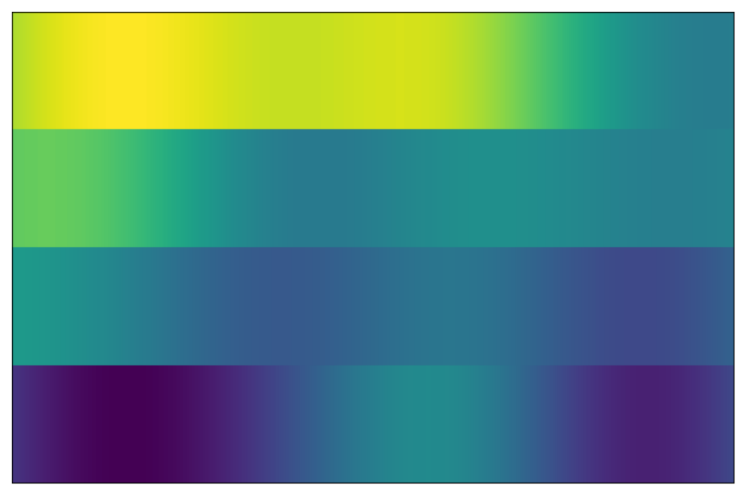
Building attention mechanisms.

We represent $f$ and $V$ using basis functions, $\phi:S\rightarrow\mathbb{R}^{M}$ and $\psi:S\rightarrow\mathbb{R}^{N}$ , defining $f_{\theta}(t)=\theta^{\top}\phi(t)$ and $V_{B}(t)=B\psi(t)$ , where $\theta\in\mathbb{R}^{M}$ and $B\in\mathbb{R}^{D\times N}$ . The scoring function $f_{\theta}$ is mapped into a probability density $p:=\hat{p}_{\Omega}[f_{\theta}]$ , from which we compute the context vector as $c=\mathbb{E}_{p}[V_{B}(t)]$ . From the definition of $V_{B}(t)$ , this is equivalent to writing $c=Br$ , where $r=\mathbb{E}_{p}[\psi(t)]$ . Summing up, we define general attention mechanisms as follows.

Definition 22 (Attention mechanism.).

Let $\langle S,\Omega,\phi,\psi\rangle$ be a tuple with $\Omega:\mathcal{M}_{+}^{1}(S)\rightarrow\mathbb{R}$ , $\phi:S\rightarrow\mathbb{R}^{M}$ , and $\psi:S\rightarrow\mathbb{R}^{N}$ . An attention mechanism on $\langle S,\Omega,\phi,\psi\rangle$ is a mapping $\rho:\Theta\subseteq\mathbb{R}^{M}\rightarrow\mathbb{R}^{N}$ , defined as:

\rho(\theta)=\mathbb{E}_{p}[\psi(t)],

(53)

with $p=\hat{p}_{\Omega}[f_{\theta}]$ and $f_{\theta}(t)=\theta^{\top}\phi(t)$ . If $\Omega=\Omega_{\alpha}$ , we call this entmax attention, denoted as $\rho_{\alpha}$ . The values $\alpha=1$ and $\alpha=2$ lead to softmax and sparsemax attention, respectively.

Example: Finite attention.

By plugging $S=\{1,...,L\}$ and $\phi(k)=\psi(k)=e_{k}$ (Euclidean canonical basis) in our Definition 22, we recover the discrete attention of Bahdanau et al. 2015. Still in the finite case, if $\phi(k)$ and $\psi(k)$ are key and value vectors and $\theta$ is a query vector, this recovers the key-value attention of Vaswani et al. 2017.

Example: Continuous attention with quadratic scoring function.

On the other hand, for $S=\mathbb{R}^{D}$ and $\phi(t)=[t,\mathrm{vec}(tt^{\top})]$ – which leads to a quadratic scoring function $f_{\theta}(t)=\theta^{\top}\phi(t)$ – we obtain new attention mechanisms (assessed experimentally for the 1-d and 2-d cases in §9): for $\alpha=1$ , the underlying density $p$ is a Gaussian, and for $\alpha=2$ , it is a truncated paraboloid (see Table 1 and §5). Intermediate cases encompass the biweight ( $\alpha=1.5$ ) and triweight ( $\alpha=4/3$ ) cases, part of the elliptical family described in §6. In all these cases, we show (Appendix G) that the expectation (53) is tractable (1-d) or simple to approximate numerically (2-d) if $\psi$ are Gaussian RBFs, and we use this fact in §9. Algorithm 1 shows pseudo-code for the case $\alpha=1$ .

Parameters: Gaussian RBFs

\psi(t)=[\mathcal{N}(t;\mu_{j},\Sigma_{j})]_{j=1}^{N}

, basis functions

\phi(t)=[t,\mathrm{vec}(tt^{\top})]

, value function

V_{B}(t)=B\psi(t)

with

B\in\mathbb{R}^{D\times N}

, scoring function

f_{\theta}(t)=\theta^{\top}\phi(t)

with

\theta\in\mathbb{R}^{M}

Function Forward( $\theta:=[\Sigma^{-1}\mu,-\frac{1}{2}\Sigma^{-1}]$ ):

r_{j}\leftarrow\mathbb{E}_{\hat{p}_{\Omega}[f_{\theta}]}[\psi_{j}(t)]=\mathcal{N}(\mu,\mu_{j},\Sigma+\Sigma_{j}),\hskip 9.24994pt\forall j\in[N]

// Eqs. (53), (147)
return $c\leftarrow Br$ (context vector)Function Backward( $\frac{\partial\mathcal{L}}{\partial c},\theta:=[\Sigma^{-1}\mu,-\frac{1}{2}\Sigma^{-1}]$ ):

for $j\leftarrow 1$ to $N$ do

\tilde{s}\leftarrow\mathcal{N}(\mu,\mu_{j},\Sigma+\Sigma_{j}),\,\,\tilde{\Sigma}\leftarrow(\Sigma^{-1}+\Sigma_{j}^{-1})^{-1},\,\,\tilde{\mu}\leftarrow\tilde{\Sigma}(\Sigma^{-1}\mu+\Sigma_{j}^{-1}\mu_{j})

\frac{\partial r_{j}}{\partial\theta}\leftarrow\mathrm{cov}_{\hat{p}_{\Omega}[f_{\theta}]}(\phi(t),\psi_{j}(t))=[\tilde{s}(\tilde{\mu}-\mu);\tilde{s}(\tilde{\Sigma}+\tilde{\mu}\tilde{\mu}^{\top}-\Sigma-\mu\mu^{\top})]

// (55), (148)-(149)
return $\frac{\partial\mathcal{L}}{\partial\theta}\leftarrow\left(\frac{\partial r}{\partial\theta}\right)^{\top}B^{\top}\frac{\partial\mathcal{L}}{\partial c}$

Algorithm 1 Continuous softmax attention:

S=\mathbb{R}^{D}

\Omega=\Omega_{1}

, Gaussian RBFs.

Defining the value function $V_{B}(t)$ .

In many problems, the input is a discrete sequence of observations (e.g., audio samples or text) or it was discretized (e.g., visual scenes), at locations $\{t_{\ell}\}_{\ell=1}^{L}$ . To turn such an input into a continuous signal, we need to smooth and interpolate these observations. If we start with a discrete encoder representing the input as a matrix $H\in\mathbb{R}^{D\times L}$ , one way of obtaining a value mapping $V_{B}:S\rightarrow\mathbb{R}^{D}$ is by “approximating” $H$ with multivariate ridge regression. With $V_{B}(t)=B\psi(t)$ , where $B\in\mathbb{R}^{D\times N}$ , and packing the basis vectors $\psi(t_{\ell})$ as columns of matrix $F\in\mathbb{R}^{N\times L}$ , we obtain:

B^{\star}\,\,=\,\,\arg\min_{B}\|BF-H\|_{F}^{2}+\lambda\|B\|_{F}^{2}\,\,=\,\,HF^{\top}(FF^{\top}+\lambda\mathrm{Id}_{N})^{-1}\,\,=\,\,HG,

(54)

where $\|\cdot\|_{F}$ is the Frobenius norm, and the $L\times N$ matrix $G=F^{\top}(FF^{\top}+\lambda\mathrm{Id}_{N})^{-1}$ depends only on the values of the basis functions at discrete time steps and can be obtained off-line for different input lenghts $L$ . The result is an expression for $V_{B}$ with $ND$ coefficients, cheaper than $H$ if $N\ll L$ .

8.2 Gradient backpropagation with continuous attention

The next proposition, based on Proposition 9 and proved in Appendix E.3, allows backpropagating over continuous entmax attention mechanisms. It uses the definition of generalized $\beta$ -covariance presented in (22) and the proof is similar to that of Proposition 11.

Proposition 23 (Jacobian expression).

Let $p=\hat{p}_{\Omega_{\alpha}}[f_{\theta}]$ with $f_{\theta}(t)=\theta^{\top}\phi(t)$ . The Jacobian of the $\alpha$ -entmax transformation $\rho_{\alpha}$ (53) is:

J_{\rho_{\alpha}}(\theta)=\frac{\partial\rho_{\alpha}(\theta)}{\partial\theta}=\mathrm{cov}_{p,2-\alpha}(\phi(t),\psi(t)).

(55)

In the finite case, (55) reduces to the expressions for the Jacobian of softmax and sparsemax derived by Martins and Astudillo 2016:

J_{\mathrm{softmax}}(f)=\mathrm{Diag}(p)-pp^{\top},\qquad J_{\mathrm{sparsemax}}(f)=\mathrm{Diag}(s)-ss^{\top}/(1^{\top}s),

(56)

where $p=\mathrm{softmax}(f)$ , and $s$ is a binary vector whose $\ell$ ^th entry is 1 iff $\ell\in\mathrm{supp}(\mathrm{sparsemax}(f))$ .

Example: Gaussian RBFs.

As before, let $S=\mathbb{R}^{D}$ , $\phi(t)=[t,\mathrm{vec}(tt^{\top})]$ , and $\psi_{j}(t)=\mathcal{N}(t;\mu_{j},\Sigma_{j})$ . For $\alpha=1$ , we obtain closed-form expressions for the expectation (53) and the Jacobian (55), for any $D\in\mathbb{N}$ : $\hat{p}_{\Omega}[f_{\theta}]$ is a Gaussian, the expectation (53) is the integral of a product of Gaussians, and the covariance (55) involves first- and second-order Gaussian moments. Pseudo-code for the case $\alpha=1$ is shown as Algorithm 1. For $\alpha=2$ , $\hat{p}_{\Omega}[f_{\theta}]$ is a truncated paraboloid. In the 1-d case, both (53) and (55) can be expressed in closed form in terms of the $\mathrm{erf}$ function. The same holds more generally if $\alpha$ is of the form $\alpha=\frac{n+1}{n}$ for $n\in\mathbb{N}$ , which includes the biweight and triweight attention cases.¹²¹² 12 This is shown in Appendix G by making use of closed-form expressions for $\int t^{n}\mathcal{N}(t;0,1)dt$ for $n\in\mathbb{N}$ . In the 2-d case, we can reduce the problem to 1-d integration by using the change of variables formula and working with polar coordinates. Appendix G derives concrete expressions.

We use the facts above in the experimental section (§9), where we experiment with $\beta$ -Gaussian attention in audio classification and vision applications.

9 Experiments

We illustrate the usefulness of the theoretical results developed in the previous sections by running experiments with continuous attention mechanisms with several choices of $\beta$ -Gaussian densities (§9.1), and on heteroscedastic regression with continuous Fenchel-Young losses (§9.2).

9.1 Continuous attention mechanisms

We test our continuous attention mechanisms on two tasks: audio classification (1-d) and visual question answering (2-d).¹³¹³ 13 All dataset statistics, architecture details, and hyperparameters are described in Appendix H.

1-d: Audio classification.

We use the UrbanSound8k dataset,¹⁴¹⁴ 14 https://urbansounddataset.weebly.com/ whose inputs are short urban sound excerpts ( $\leq 4s$ ) from 10 classes: air conditioner, car horn, children playing, dog bark, drilling, engine idling, gun shot, jackhammer, siren, and street music. We use a 16kHz sampling rate for all audios. We transform the input signal into a sequence of vectors using short-time Fourier transform with 400 points, a window size of 25ms, and a hop size of 10ms. After this transformation, we extract 80 Mel-frequency filter banks by applying equally-spaced triangular filters. Our baseline is a model with a single convolutional 1-d layer followed by a discrete attention mechanism and an output layer. For our continuous attention models, we normalize the input signal length $L$ into the unit interval $[0,1]$ , and use $f(t)\!=\!\nicefrac{{-(t-\mu)^{2}}}{{2\sigma^{2}}}$ as the score function. Continuous attention models obtain $p\in\triangle^{L}$ from discrete attention, compute $\mu=\mathbb{E}_{p}[\ell/L]$ and $\sigma^{2}=\mathbb{E}_{p}[(\ell/L)^{2}]-\mu^{2}$ , apply the continuous attention transformation, and sum the two context vectors (this model has the same number of parameters as the discrete attention baseline).

Since the dataset is officially split into 10 folds, we perform 10-fold cross-validation to evaluate our models. Table 3 shows accuracies for different values of $\alpha$ and the standard deviation across folds. The models with continuous attention perform better than the baselines, suggesting that adding a continuous mechanism improves its discrete counterpart without increasing the number of parameters. There is no clear winner among the different choices of $\alpha$ , with all models performing similar. However, we notice that sparser choices ( $\alpha>1$ ) lead to more interpretable predictions, as shown in Figure 10.

Table 3: Results on UrbanSound8k in terms of accuracy. For continuous attention, we used

128

Gaussian RBFs

\mathcal{N}(t,\tilde{\mu},\tilde{\sigma}^{2})

, with

\tilde{\mu}

linearly spaced in

[0,1]

and

\tilde{\sigma}\in\{.1,.5\}

Attention	$\alpha=1.0$	$\alpha=4/3$	$\alpha=1.5$	$\alpha=2.0$
Discrete	0.5967 ± 0.06	0.5946 ± 0.07	0.6032 ± 0.05	0.5903 ± 0.05
Continuous	0.6229 ± 0.06	0.6280 ± 0.06	0.6171 ± 0.05	0.6247 ± 0.06

2-d: Visual QA.

We report experiments with 2-d continuous attention on visual question answering, using the VQA-v2 dataset (Goyal et al. 2019) and a modular co-attention network as a baseline (Yu et al. 2019). The discrete attention model attends over a 14 $\times$ 14 grid. For continuous attention, we normalize the image size into the unit square $[0,1]^{2}$ . We fit a 2-d Gaussian ( $\alpha=1$ ) or truncated paraboloid ( $\alpha=2$ ) as the attention density; both correspond to $f(t)=-\frac{1}{2}(t-\mu)^{\top}\Sigma^{-1}(t-\mu)$ , with $\Sigma\succ 0$ . We use the mean and variance according to the discrete attention probabilities and obtain $\mu$ and $\Sigma$ with moment matching (using the variance formula from Proposition 17). We use $N=100\ll 14^{2}$ Gaussian RBFs, with $\tilde{\mu}$ linearly spaced in $[0,1]^{2}$ and $\tilde{\Sigma}=0.001\cdot\mathrm{Id}$ . Overall, the number of neural network parameters is the same as in discrete attention.

The results in Table 4 show similar accuracies for all attention models, with a slight advantage for continuous softmax. Figure 11 shows two examples (see Appendix H for more examples and some failure cases): in both examples, the discrete attention is too scattered, possibly mistaking the lamp with a TV screen in the first example. The continuous attention models focus on the right region and answer the questions correctly, with continuous sparsemax enclosing all the relevant information in its supporting ellipse.

Table 4: Accuracies of different models on the test-dev and test-standard splits of VQA-v2.

Attention	Test-Dev				Test-Standard
	Yes/No	Number	Other	Overall	Yes/No	Number	Other	Overall
Discrete softmax	83.40	43.59	55.91	65.83	83.47	42.99	56.33	66.13
2-d continuous softmax	83.40	44.80	55.88	65.96	83.79	44.33	56.04	66.27
2-d continuous sparsemax	83.10	44.12	55.95	65.79	83.38	43.91	56.14	66.10

9.2 Heteroscedastic regression with Fenchel-Young losses

Regression is often tackled using a squared loss, which is equivalent to assuming a one-dimensional normal distribution for the target variable. In this experiment, we explore replacing this normal distribution with a $\beta$ -Gaussian, where not only the mean but also the variance of the residuals is also allowed to depend on the features. We analyze the Breast Cancer Mortality and Population dataset from Rice 2006, accessed via statsmodels (Seabold and Perktold 2010). The data covers 301 counties in southern US. The single input variable $x$ is the population of the county, and the target variable $y$ is the breast cancer mortality rate. As more populous counties display more variability, a standard linear model fit on the full dataset shows strong signs of heteroscedasticity according to a Breusch-Pagan test ( $LM=537.4,p<10^{-118}$ ).

Experimental setup.

We leave out the $10\%$ most populous counties as a test set, and fit a linear model with $\beta$ -Gaussian data-dependent noise,

y\sim\mu_{f}(x)+\mathcal{N}_{\beta}(0,\sigma_{f}^{2}(x)),\qquad\text{where}\qquad\begin{array}[]{rl}\mu_{f}(x)&\coloneqq w_{\mu}\cdot x+b_{\mu},\\ \sigma^{2}_{f}(x)&\coloneqq(w_{\sigma}\cdot x+b_{\sigma})^{2}\,.\end{array}

(57)

(Note that $\sigma_{f}^{2}$ is not linear in $x$ .) We first fit a baseline standard linear regression, i.e., $y\sim\mu_{f}\cdot x+\mathcal{N}(0,1)$ , and initialize $w_{\mu}$ and $b_{\mu}$ in all subsequent models with the baseline values. We apply 1000 iterations of L-BFGS with a step size of $.01$ to minimize the average cross- $\Omega$ loss $L^{\times}_{\Omega}$ against a target Dirac limit case $p=\delta_{y}$ (Definition 3, Proposition 18), which in the 1-d case simplifies to:

L^{\times}_{\Omega_{\alpha}}(\mu_{f},\sigma_{f}^{2},y)=\frac{(\mu_{f}-y)^{2}}{2\sigma_{f}^{2}}-\frac{R^{2}}{2(\sigma_{f}^{2})^{\frac{\alpha-1}{\alpha+1}}}\cdot\frac{\alpha-1}{3\alpha-1}+\frac{1}{\alpha(\alpha-1)}\,,

(58)

Results.

We report explained variance ( $r^{2}$ ) in Table 5. Modeling $\sigma^{2}$ improves over the baseline, especially with $\alpha=2$ . The fit is illustrated in Figure 12 alongside the Gaussian ( $\alpha=1$ ) case. The results demonstrate that the $\beta$ -Gaussian family is useful in modeling, and that $L^{\times}_{\Omega}$ is an appropriate generalization of cross-entropy.

Table 5: Heteroscedastic regression test

r^{2}

: proportion of variance explained by

\beta

-Gaussian regression models with learned variance.

Baseline	$\alpha=1.0$	$\alpha=4/3$	$\alpha=1.5$	$\alpha=2.0$
0.56	0.67	0.68	0.69	0.72

Figure 12: Heteroscedastic regression models with a

\beta

-Gaussian model. The truncated parabola model achieves the best generalization out of the considered models in terms of

r^{2}

. For

\alpha>1

, the bounded support can be computed using Proposition 16. Note that, for

\alpha=2

, even though some points lie outside of the modeled support, the likelihood of the model is zero but the cross-

\Omega

Fenchel-Young loss is finite and learns good regressors.

10 Related Work

Generalized exponential families and loss functions.

Grünwald and Dawid 2004 introduced generalized exponential families as maximum entropy distributions for generalized entropy functions. Based upon these results, Frongillo and Reid 2014 study generalized exponential families (possibly in infinite spaces) from a convex duality perspective. Their main result is a generalization of the well-known bijection between Bregman divergences and regular exponential families. Amari et al. 2012 study deformed exponential families, including their entropy and canonical divergence. Fenchel-Young losses are closely related to proper scoring rules (Gneiting and Raftery 2007; Reid and Williamson 2010; Williamson et al. 2016). Proper scoring rules can be seen as primal-space Bregman divergences, while Fenchel-Young losses can be seen as mixed-space Bregman divergences (Blondel et al. 2020). Mensch et al. 2019 propose a Fenchel-Young loss in the continuous setting. Their focus, however, is on a geometric notion of entropy called “Sinkhorn entropy”. Blondel 2019 studies the consistency of a subset of Fenchel-Young losses. In this paper, we provide a throrough study of generalized continuous distributions and losses from a convex duality perspective with a particular focus on distributions with sparse support. In doing so, we unify many continuous distributions and create new ones seamlessly. We also discuss their Jacobian computation, enabling their use in a neural network trained by backpropagation.

Nock and Nielsen 2009 proposed a binary classification loss construction based on the Legendre transformation but their construction precludes non-invertible mappings. Duchi et al. 2018 derived a multi-class loss which is a special case of Fenchel-Young loss over the probability simplex. Nowak-Vila et al. 2020 use Fenchel-Young losses to construct a new loss with a max-min margin property. This loss corresponds to choosing $\alpha\to\infty$ in the Tsallis negentropy. Finally, Bao and Sugiyama 2021 used Fenchel-Young losses to derive new losses for class-posterior probability estimation with unbalanced classes. All these works are limited to the finite output domains.

The regularized prediction map presented in §2 is connected to proximal operators (Moreau 1965). Indeed, if $\Omega=\frac{1}{2}\|\cdot\|^{2}_{2}+\Phi$ , then $\hat{p}_{\Omega}[f]=\text{prox}_{\Phi}$ (Blondel et al. 2020). At a high level, the Fenchel-Young loss in §3 resembles formulations for structured prediction (Taskar et al. 2005) which formulate learning as the problem of finding a saddle point involving a game between the model parameters (corresponding to our $f_{\theta}$ ) and marginal probabilities for structured outputs (corresponding to our $p$ ). The focus of our paper, however, is on continuous domains rather than structured prediction.

Relation to the Tsallis maxent principle.

Our paper unifies two lines of work: deformed exponential families from statistical physics (Tsallis 1988; Naudts 2009; Amari and Ohara 2011), and sparse alternatives to softmax recently proposed in the machine learning literature (Martins and Astudillo 2016; Peters et al. 2019; Blondel et al. 2020), herein extended to continuous domains. This link may be fruitful for future research in both fields. While most prior work is focused on heavy-tailed distributions ( $\alpha<1$ ), we focus instead on light-tailed, sparse distributions, the other side of the spectrum ( $\alpha>1$ ). See Appendix C.4 for the relation to the Tsallis maxent principle.

Continuity in other architectures and dimensions.

In our paper, we consider attention networks exhibiting temporal/spatial continuity in the input data, be it audio signals (1-d) or visual scenes (2-d). Recent works propose continuous-domain CNNs for 3-d structures like point clouds and molecules (Wang et al. 2018; Schütt et al. 2017). The dynamics of continuous-time RNNs have been studied in (Funahashi and Nakamura 1993), and similar ideas have been applied to irregularly sampled time series (Rubanova et al. 2019). Other recently proposed frameworks produce continuous variants in other dimensions, such as network depth (Chen et al. 2018), or in the target domain for machine translation tasks (Kumar and Tsvetkov 2018). Our continuous attention networks can be used in tandem with these frameworks.

Gaussian attention probabilities.

Cordonnier et al. 2019 analyze the relationship between (discrete) attention and convolutional layers, and consider spherical Gaussian attention probabilities as relative positional encodings. By contrast, our approach removes the need for positional encodings: by converting the input to a function on a predefined continuous space, positions are encoded implicitly, not requiring explicit positional encoding. Gaussian attention has also been hard-coded as input-agnostic self-attention layers in transformers for machine translation tasks by You et al. 2020. Finally, in their DRAW architecture for image generation, Gregor et al. 2015 propose a selective attention component which is parametrized by a spherical Gaussian distribution.

Sparse latent variables.

Related to the sparse attention models developed in §8, several works have presented models with sparse latent variables, mostly for the discrete (possibly structured) case, both in deterministic (Correia et al. 2020; Guerreiro and Martins 2021) and stochastic settings (Bastings et al. 2019; Farinhas et al. 2022). Generalizing these constructions to continuous latent variables with sparse support (in the sense of Definition 1) is an interesting direction for future work.

11 Conclusions and Future Work

We extended $\Omega$ -regularized prediction maps and Fenchel-Young losses to arbitrary measure spaces (§2, §3). A key result is that, for linearly parametrized families, Fenchel-Young loss minimization is equivalent to moment matching of the statistics, generalizing the concept of sufficient statistics from exponential families (Proposition 6). With Tsallis $\alpha$ -entropies for $\alpha>1$ , we obtain sparse families, whose members can have zero tails, such as triangular or truncated parabola/paraboloid distributions on continuous domains or sparse integer distributions in discrete but infinite domains, for $\alpha=2$ (§4, §5). We provided a general characterization of the normalizing function $A_{\alpha}(f)$ , its gradient and Hessian, and expressions for the Fenchel-Young loss for arbitrary $\alpha$ (Propositions 8, 9, 10, and 11). We then studied the particular case of $\beta$ -Gaussian distributions, induced by Tsallis $\alpha$ -entropies (with $\beta=2-\alpha$ ) and quadratic scoring functions, and we have shown that they are instances of elliptical distributions (§6), containing as particular cases the Gaussian and truncated paraboloid, as providing multivariate generalizations of distributions commonly used in kernel density estimation (Epanechnikov, biweight, triweight). We have shown that these distributions can be reparametrized by two independent random variables, a Beta distribution for the radius, and a uniform spherical distribution (Proposition 16), and used this result to build an efficient sampler. We also characterized key properties of these distributions: their mean, variance, entropy, and a closed-form for the Fenchel-Young loss (Propositions 17–18). The combination of the sampler and estimation with Fenchel-Young loss minimization using these results is illustrated in Figure 4. Finally, we have shown that by considering total variance and Sobolev regularizers $\Omega$ , regularized prediction maps allow building continuous counterparts of the fusedmax transformation previously proposed in the discrete case (§7).

In a nutshell, the theoretical contributions of our paper unify two lines of work: deformed exponential families from statistical physics (Tsallis 1988; Naudts 2009; Amari and Ohara 2011), and sparse alternatives to softmax recently proposed in the machine learning literature (Martins and Astudillo 2016; Niculae and Blondel 2017; Peters et al. 2019; Blondel et al. 2020). We frame this unification in the scope of regularized prediction maps (a generalization of the variational free energy principle) and Fenchel-Young losses (a generalization of Kullback-Leibler divergences and Bregman divergences). We believe this link may be fruitful for future research in both fields. While most prior work is focused on heavy-tailed distributions ( $\alpha<1$ ), we focus instead on light-tailed, sparse distributions, the other side of the spectrum ( $\alpha>1$ ).

We have also shown how $\Omega$ -regularized predictions maps can be used in neural network models to construct continuous attention mechanisms (§8), generalizing finite attention (Bahdanau et al. 2015) to continuous input data, such as 1-d spatial or temporal signals or 2-d images (visual scenes). We derived their Jacobians in terms of generalized covariances (Proposition 23), allowing for efficient forward and backward propagation. Experiments for 1-d and 2-d cases were shown on attention-based audio classification and visual question answering (§9).

There are many avenues for future work. The sparse integer distributions presented in §5 open up interesting questions, such as the efficient computation of key quantities (mean, entropies, Fenchel-Young loss) and its applicability to problems that could benefit from distributions with finite but varying support (ranges). Likewise, the $\beta$ -Gaussian distributions presented in §6 might be useful in embedding spaces, where objects (e.g., words) could be modeled as compact sets. Our results concerning $\Omega$ -regularized prediction maps and Fenchel-Young losses provided in §2–3 are very general, and it is plausible that regularizers $\Omega$ other than Tsallis entropies, total variation or Sobolev regularizers might be useful. While our paper focused on linearly parametrized energy functions, the non-linear case (e.g., where $f(t)$ is obtained from a neural network) deserves further study—in fact, several of our theoretical results can be easily extended to this case by replacing $\phi(t)$ by $\nabla_{\theta}f_{\theta}(t)$ . Regarding sparse continuous attention mechanisms, while our paper focused on unimodal distributions, there are applications in which multiple attention modes are desirable. This can be done by considering mixtures of distributions, multiple attention heads, or sequential attention steps. Initial work in that direction includes Farinhas et al. 2021. Another direction concerns combining our continuous attention models with other spatial/temporal continuous architectures for CNNs and RNNs (Wang et al. 2018; Schütt et al. 2017; Funahashi and Nakamura 1993) or with continuity in other dimensions, such as depth (Chen et al. 2018) or output space (Kumar and Tsvetkov 2018). Recent work using continuous attention mechanisms to model long-term “sticky” memories in transformer architectures has been done by Martins et al. 2022; some of the ideas above are applicable there, too.

acknowledgments-disclosure-of-funding.

We thank the action editor and the anonymous reviewers for their insightful comments and suggestions. This work was supported by the European Research Council (ERC StG DeepSPIN 758969) and by the Fundação para a Ciência e Tecnologia through project PTDC/CCI-INF/4703/2021 (PRELUNA) and contract UIDB/50008/2020 and in part by the Hybrid Intelligence Centre, a 10-year program funded by the Dutch Ministry of Education, Culture, and Science through the Netherlands Organisation for Scientific Research (https://hybrid-intelligence-centre.nl).

Appendix

Appendix A Proofs for regularized prediction maps

A.1 Equivariance of distributions

Let $S=\mathbb{R}^{N}$ and $\nu$ be the Lebesgue measure. We show that, if the regularizer $\Omega$ is separable (i.e. if it can be written as $\Omega(p)=\int_{S}\psi(p(t))$ for some function $\psi:\mathbb{R}_{+}\rightarrow\mathbb{R}$ ), the following equivariance property holds:

\hat{p}_{\Omega}[\tilde{f}](t)=\hat{p}_{\Omega}[f](At+b),

(59)

where $\tilde{f}(t):=f(At+b)$ , for any matrix $A$ with determinant $\pm 1$ and any vector $b\in\mathbb{R}^{N}$ .

By definition, we have

\hat{p}_{\Omega}[\tilde{f}]=\argmax_{p\in\mathcal{M}_{+}^{1}(\mathbb{R}^{N})}\mathbb{E}_{p}[\tilde{f}(t)]-\Omega(p)=\argmax_{p\in\mathcal{M}_{+}^{1}(\mathbb{R}^{N})}\int_{S}(p(t)\,f(At+b)-\psi(p(t))\,dt.

(60)

Making a change of variables $s=At+b$ , using the change of variables’ formula (noting that $|\det(A)|=1$ ), and defining $q(s)=p(A^{-1}(s-b))$ – noting that $p\in\mathcal{M}_{+}^{1}(\mathbb{R}^{N})$ iff $q\in\mathcal{M}_{+}^{1}(\mathbb{R}^{N})$ – we obtain:

	$\displaystyle\hat{p}_{\Omega}[\tilde{f}](t)$	$\displaystyle=$	$\displaystyle\left(\argmax_{q\in\mathcal{M}_{+}^{1}(\mathbb{R}^{N})}\int_{S}(q(s)\,f(s)-\psi(q(s))\,ds\right)(s)=\left(\argmax_{q\in\mathcal{M}_{+}^{1}(\mathbb{R}^{N})}\mathbb{E}_{q}[f(s)]-\Omega(q)\right)(s)$		(61)
		$\displaystyle=$	$\displaystyle\hat{p}_{\Omega}[f](s),$		(61)

which leads to the desired result.

A.2 Differential Negentropy and Boltzmann-Gibbs distributions

We adapt a proof from Cover and Thomas 2012. Let $\Omega$ be the Shannon negentropy, which is proper, lower semi-continuous, and strictly convex (Bauschke and Combettes 2011, example 9.41), and let

\mathrm{KL}(p\|q):=\int_{S}p(t)\log\frac{p(t)}{q(t)}

be the Kullback-Leibler divergence between distributions $p$ and $q$ (which is always non-negative and equals $0$ iff $p=q$ ). Take $q(t)=\frac{\exp(f(t))}{\int_{S}\exp(f(t^{\prime}))d\nu(t^{\prime})}=\exp(f(t)-A(f))$ as in (3), where $A(f)$ is the log-partition function.

We have, for any $p\in\mathcal{M}_{+}^{1}(S)$ :

	$\displaystyle 0$	$\displaystyle\leq$	$\displaystyle\mathrm{KL}(p\\|q)=\int_{S}p(t)\log\frac{p(t)}{q(t)}=\Omega(p)-\int_{S}p(t)\log q(t)=\Omega(p)-\int_{S}p(t)(f(t)-A(f))$		(62)
		$\displaystyle=$	$\displaystyle\Omega(p)-\mathbb{E}_{p}[f(t)]+A(f).$		(62)

Therefore, we have, for any $p\in\mathcal{M}_{+}^{1}(S)$ , that

\mathbb{E}_{p}[f(t)]-\Omega(p)\leq A(f),

(63)

with equality if and only if $p=q$ . Since the right hand side is constant with respect to $p$ , we have that the posited $q$ must be the maximizer of (2).

Appendix B Proofs for continuous Fenchel-Young losses

Proof of Propositions 4–6

The proof of Proposition 4 adapts that of Blondel et al. 2020 when Fenchel duality is now taken in the infinite-dimensional set $\mathcal{F}\subseteq\mathbb{R}^{S}$ , which endowed with the inner product $\langle f,g\rangle=\int_{S}f(t)g(t)d\nu(t)$ forms a Hilbert space (Bauschke and Combettes 2011). The non-negativity of $L_{\Omega}$ stems from the Fenchel-Young inequality in Hilbert spaces. The loss is zero iff $(f_{\theta},p)$ is a dual pair, i.e., if $p=\hat{p}_{\Omega}[f_{\theta}]=\nabla\Omega^{*}(f_{\theta})$ .

To prove Proposition 5, note that the gradient of $L_{\Omega}$ is

\nabla_{\theta}L_{\Omega}(f_{\theta};p)=\int_{S}\frac{\partial L_{\Omega}(f_{\theta};p)}{\partial f_{\theta}(t)}\nabla_{\theta}f_{\theta}(t)d\nu(t)=\int_{S}(\hat{p}_{\Omega}[f_{\theta}](t)-p(t))\nabla_{\theta}f_{\theta}(t),

where we used the fact that $\frac{\partial L_{\Omega}(f_{\theta};p)}{\partial f_{\theta}(t)}=[\nabla\Omega^{*}(f_{\theta})-p](t)$ . This leads to the expression in (7).

The first point in Proposition 6 is a direct consequence of the last result. The convexity of $L_{\Omega}$ with respect to $\theta$ stems from the fact that $L_{\Omega}(f_{\theta},p)=\Omega(p)+\Omega^{*}(f_{\theta})-\mathbb{E}_{p}[f_{\theta}(t)]$ is convex with respect to $f_{\theta}$ (since it is the sum of an affine function with $\Omega^{*}(f_{\theta})$ , which, being a Fenchel dual, is convex) and that $L_{\Omega}$ , as a function of $\theta$ , is a composition of the linear mapping $\theta\mapsto f_{\theta}(\cdot)=\theta^{\top}\phi(\cdot)$ with the said convex function, hence it is convex. Finally, the last statement is an immediate consequence of the two previous claims: Since $L_{\Omega}$ is convex, any stationary point is a global minimum, and, from the first claim, any stationary point $\hat{\theta}$ must satisfy $\mathbb{E}_{\hat{p}_{\Omega}[f_{\hat{\theta}}]}[\phi(t)]=\mathbb{E}_{p}[\phi(t)]$ .

Appendix C Proofs for Tsallis regularization and Deformed Exponential Families

C.1 Shannon as a limit case of Tsallis when $\alpha\rightarrow 1$

We show that $\lim_{\alpha\rightarrow 1}\Omega_{\alpha}(p)=\Omega_{1}(p)$ for any $p\in\mathcal{M}_{+}^{1}(S)$ . From (14), it suffices to show that $\lim_{\beta\rightarrow 1}\log_{\beta}(u)=\log(u)$ for any $u\geq 0$ . Let $g(\beta)\coloneqq u^{1-\beta}-1$ , and $h(\beta)\coloneqq 1-\beta$ . Observe that

\lim_{\beta\rightarrow 1}\log_{\beta}(u)=\lim_{\beta\rightarrow 1}\frac{g(\beta)}{h(\beta)}=\frac{g(1)}{h(1)}=\frac{0}{0},

so we are in an indeterminate case. We take the derivatives of $g$ and $h$ :

g^{\prime}(\beta)=\left(\exp(\log u^{1-\beta})\right)^{\prime}=\exp(\log u^{1-\beta})\cdot((1-\beta)\log u)^{\prime}=-u^{1-\beta}\log u,

(64)

and $h^{\prime}(\beta)=-1$ . From l’Hôpital’s rule,

\lim_{\beta\rightarrow 1}\frac{g(\beta)}{h(\beta)}=\lim_{\beta\rightarrow 1}\frac{g^{\prime}(\beta)}{h^{\prime}(\beta)}=\log u.

(65)

C.2 Proof of Proposition 8

The proof of Proposition 8 is similar to the one in §A.2, replacing the KL divergence by the Bregman divergence induced by $\Omega_{\alpha}$ , and using an additional bound. Let

B_{\Omega_{\alpha}}(p,q):=\Omega_{\alpha}(p)-\Omega_{\alpha}(q)-\langle\nabla\Omega_{\alpha}(q),p-q\rangle

be the (functional) Bregman divergence between distributions $p$ and $q$ induced by $\Omega_{\alpha}$ , and let

q(t)=\exp_{2-\alpha}(f(t)-A_{\alpha}(f))=[1+(\alpha-1)(f(t)-A_{\alpha}(f))]_{+}^{\frac{1}{\alpha-1}}.

Note that, from (14),

\left(\nabla_{q}\Omega_{\alpha}(q)\right)(t)=\frac{q(t)^{\alpha-1}}{\alpha-1}.

From the non-negativity of the Bregman divergence Bregman 1967, we have, for any $p\in\mathcal{M}_{+}^{1}(S)$ :

$\displaystyle 0$	$\displaystyle\leq^{(a)}$	$\displaystyle B_{\Omega_{\alpha}}(p,q)$	(66)
	$\displaystyle=$	$\displaystyle\Omega_{\alpha}(p)-\Omega_{\alpha}(q)-\langle\nabla\Omega_{\alpha}(q),p-q\rangle$
	$\displaystyle=$	$\displaystyle\Omega_{\alpha}(p)-\Omega_{\alpha}(q)-\int_{S}\frac{q(t)^{\alpha-1}}{\alpha-1}(p(t)-q(t))$
	$\displaystyle=$	$\displaystyle\Omega_{\alpha}(p)-\Omega_{\alpha}(q)-\underbrace{\mathbb{E}_{p}[[f(t)-A_{\alpha}(f)+(\alpha-1)^{-1}]_{+}]}_{\geq\mathbb{E}_{p}[f(t)-A_{\alpha}(f)+(\alpha-1)^{-1}]}+\frac{1}{\alpha-1}\int_{S}q(t)^{\alpha}$
	$\displaystyle\leq^{(b)}$	$\displaystyle\Omega_{\alpha}(p)-\Omega_{\alpha}(q)-\mathbb{E}_{p}[f(t)-A_{\alpha}(f)+(\alpha-1)^{-1}]+\frac{1}{\alpha-1}\int_{S}q(t)^{\alpha}$
	$\displaystyle=$	$\displaystyle\Omega_{\alpha}(p)-\mathbb{E}_{p}[f(t)]-\Omega_{\alpha}(q)+\underbrace{\frac{1}{\alpha-1}\left(\int_{S}q(t)^{\alpha}-1\right)}_{=\alpha\Omega_{\alpha}(q)}+A_{\alpha}(f)$
	$\displaystyle=$	$\displaystyle\Omega_{\alpha}(p)-\mathbb{E}_{p}[f(t)]+(\alpha-1)\Omega_{\alpha}(q)+A_{\alpha}(f).$

Therefore, we have, for any $p\in\mathcal{M}_{+}^{1}(S)$ ,

\mathbb{E}_{p}[f(t)]-\Omega_{\alpha}(p)\leq(\alpha-1)\Omega_{\alpha}(q)+A_{\alpha}(f),

(67)

with equality iff $p=q$ , which leads to zero Bregman divergence (i.e., a tight inequality $(a)$ ) and to $\mathbb{E}_{p}[[f(t)-A_{\alpha}(f)+(\alpha-1)^{-1}]_{+}]=\mathbb{E}_{p}[f(t)-A_{\alpha}(f)+(\alpha-1)^{-1}]$ (i.e., a tight inequality $(b)$ ).

We can use the equality above to obtain an expression for the Fenchel conjugate $\Omega_{\alpha}^{*}(f)=\mathbb{E}_{q}[f(t)]-\Omega_{\alpha}(q)$ (i.e., the value of the maximum in (2) and the right hand side in (67)):

\Omega_{\alpha}^{*}(f)=(\alpha-1)\Omega_{\alpha}(q)+A_{\alpha}(f).

(68)

C.3 Normalizing function $A_{\alpha}(f)$

Let $p=\hat{p}_{\Omega_{\alpha}}[f]$ . The expression for $A_{\alpha}$ in Prop. 8 is obtained by inverting (15), yielding $A_{\alpha}(f)=f(t)-\log_{2-\alpha}(p(t))$ , and integrating with respect to $p(t)^{2-\alpha}d\nu(t)$ , leading to:

$\displaystyle\int_{S}p(t)^{2-\alpha}A_{\alpha}(f)$	$\displaystyle=$	$\displaystyle\int_{S}p(t)^{2-\alpha}f(t)-\int_{S}p(t)^{2-\alpha}\log_{2-\alpha}(p(t))$	(69)
	$\displaystyle=$	$\displaystyle\int_{S}p(t)^{2-\alpha}f(t)-\frac{\int_{S}(p(t)-p(t)^{2-\alpha})}{\alpha-1}$
	$\displaystyle=$	$\displaystyle\int_{S}p(t)^{2-\alpha}f(t)-\frac{1}{\alpha-1}+\frac{\int_{S}p(t)^{2-\alpha}}{\alpha-1},$

from which the desired expression follows.

C.4 Relation to the Tsallis Maxent Principle

We discuss here the relation between the $(2-\alpha)$ -exponential family of distributions as presented in Prop. 8 and the distributions arising from the Tsallis maxent principle (Tsallis 1988). We put in perspective the related work in statistical physics (Abe 2003; Naudts 2009), information geometry (Amari and Ohara 2011; Amari 2016), and the discrete case presented in the machine learning literature (Blondel et al. 2020; Peters et al. 2019).

We start by noting that our $\alpha$ parameter matches the $\alpha$ used in prior machine learning literature related to the “ $\alpha$ -entmax transformation” (Blondel et al. 2020; Peters et al. 2019). In the definition of Tsallis entropies (14), our $\alpha$ corresponds to the entropic index $q$ defined by Tsallis 1988. However, our $(2-\alpha)$ -exponential families correspond to the $q$ -exponential families as defined by Naudts 2009, and to the $t$ -exponential families described by Ding and Vishwanathan 2010 (which include the $t$ -Student distribution). The family of Amari’s $\alpha$ -divergences relates to this $q$ as $\alpha=2q-1$ (Amari 2016, §4.3).

These differences in notation have historical reasons, and they are explained by the different ways in which Tsallis entropies relate to $q$ -exponential families. In fact, the physics literature has defined $q$ -exponential distributions in two distinct ways, as we next describe.

Note first that the $\Omega$ -regularized prediction map in our Def. 2 is a generalization of the free energy variational principle, if we see $-f_{\theta}(t)=-\theta^{\top}\phi(t)$ as an energy function and $\Omega$ the entropy scaled by a temperature. Let $\Omega=\Omega_{\alpha}$ be the Tsallis $\alpha$ -entropy. An equivalent constrained version of this problem is the maximum entropy (maxent) principle (Jaynes 1957):

\max_{p\in\mathcal{M}_{+}^{1}(S)}-\Omega_{\alpha}(p),\hskip 14.22636pt\mathrm{s.t.}\hskip 9.95863pt\mathbb{E}_{p}[\phi(t)]=b.

(70)

The solution of this problem corresponds to a distribution in the $(2-\alpha)$ -exponential family (15):

p^{\star}(t)=\exp_{2-\alpha}(\theta^{\top}\phi(t)-A_{\alpha}(\theta)),

(71)

for some Lagrange multiplier $\theta$ .

However, this construction differs from the one by Tsallis 1988 and others, who use escort distributions (13) in the expectation constraints. Namely, instead of (70), they consider the problem:

\max_{p\in\mathcal{M}_{+}^{1}(S)}-\Omega_{\alpha}(p),\hskip 14.22636pt\mathrm{s.t.}\hskip 9.95863pt\mathbb{E}_{{\color[rgb]{0,0,1}\tilde{p}^{\alpha}}}[\phi(t)]=b.

(72)

The solution of (72) is of the form

p^{\star}(t)=B_{\alpha}(\theta)\exp_{\alpha}(\theta^{\top}(\phi(t)-b)),

(73)

where $\theta$ is again a Lagrange multiplier. This is derived, for example, in (Abe 2003, Eq. 15). There are two main differences between (71) and (73):

•

While (71) involves the $(2-\alpha)$ -exponential, (73) involves the $\alpha$ -exponential.
•

In (71), the normalizing term $A_{\alpha}(\theta)$ is inside the $(2-\alpha)$ -exponential. In (73), there is an normalizing factor $B_{\alpha}(\theta)$ outside the $\alpha$ -exponential.

Naturally, when $\alpha=1$ , these two problems become equivalent, since an additive term inside the exponential is equivalent to a multiplicative term outside. However, this does not happen with $\beta$ -exponentials ( $\exp_{\beta}(u+v)\neq\exp_{\beta}(u)\exp_{\beta}(v)$ in general, for $\beta\neq 1$ ), and therefore these two alternative paths lead to two different definitions of $q$ -exponential families. Unfortunately, both have been considered in the physics literature, under the same name, and this has been subject of debate. Quoting Naudts 2009:

“An important question is then whether in the modification the normalization should stand in front of the deformed exponential function, or whether it should be included as $\ln Z(\beta)$ inside. From the general formalism mentioned above it follows that the latter is the right way to go.”

Throughout our paper, we use the definition of (Naudts 2009; Amari and Ohara 2011), equivalent to the maxent problem (70).

C.5 Proof of Proposition 9

We adapt the proof from Amari and Ohara 2011. Note first that, for $t\in\mathrm{supp}(p_{\theta})$ ,

$\displaystyle\nabla_{\theta}p_{\theta}(t)$	$\displaystyle=$	$\displaystyle\nabla_{\theta}[(\alpha-1)(\theta^{\top}\phi(t)-A_{\alpha}(\theta))+1]^{1/(\alpha-1)}$	(74)
	$\displaystyle=$	$\displaystyle[(\alpha-1)(\theta^{\top}\phi(t)-A_{\alpha}(\theta))+1]^{(2-\alpha)/(\alpha-1)}(\phi(t)-\nabla_{\theta}A_{\alpha}(\theta))$
	$\displaystyle=$	$\displaystyle p_{\theta}(t)^{2-\alpha}(\phi(t)-\nabla_{\theta}A_{\alpha}(\theta)),$

and

$\displaystyle\nabla^{2}_{\theta}p_{\theta}(t)$	$\displaystyle=$	$\displaystyle\nabla_{\theta}p_{\theta}^{2-\alpha}(t)(\phi(t)-\nabla_{\theta}A_{\alpha}(\theta))^{\top}-p_{\theta}^{2-\alpha}(t)\nabla^{2}_{\theta}A_{\alpha}(\theta)$	(75)
	$\displaystyle=$	$\displaystyle(2-\alpha)p_{\theta}^{1-\alpha}(t)\nabla_{\theta}p_{\theta}(t)(\phi(t)-\nabla_{\theta}A_{\alpha}(\theta))^{\top}-p_{\theta}^{2-\alpha}(t)\nabla^{2}_{\theta}A_{\alpha}(\theta)$
	$\displaystyle=$	$\displaystyle(2-\alpha)p_{\theta}(t)^{3-2\alpha}\bigl(\phi(t)-\nabla_{\theta}A_{\alpha}(\theta)\bigr)\bigl(\phi(t)-\nabla_{\theta}A_{\alpha}(\theta)\bigr)^{\top}$
		$\displaystyle-p_{\theta}(t)^{2-\alpha}\nabla^{2}_{\theta}A_{\alpha}(\theta).$

Therefore we have:

0=\nabla_{\theta}\underbrace{\int_{S}p_{\theta}(t)}_{=1}=\int_{S}\nabla_{\theta}p_{\theta}(t)=\int_{S}p_{\theta}(t)^{2-\alpha}(\phi(t)-\nabla_{\theta}A_{\alpha}(\theta)),

(76)

from which we obtain

\nabla_{\theta}A_{\alpha}(\theta)=\frac{\int_{S}p_{\theta}(t)^{2-\alpha}\phi(t)}{\int_{S}p_{\theta}(t)^{2-\alpha}}.

(77)

To prove that $A_{\alpha}(\theta)$ is convex, we will show that its Hessian is positive semidefinite. Note that

$\displaystyle 0$	$\displaystyle=$	$\displaystyle\nabla^{2}_{\theta}\underbrace{\int_{S}p_{\theta}(t)}_{=1}=\int_{S}\nabla^{2}_{\theta}p_{\theta}(t)$	(78)
	$\displaystyle=$	$\displaystyle\int_{S}(2-\alpha)p_{\theta}(t)^{3-2\alpha}\bigl(\phi(t)-\nabla_{\theta}A_{\alpha}(\theta)\bigr)\bigl(\phi(t)-\nabla_{\theta}A_{\alpha}(\theta)\bigr)^{\top}-p_{\theta}(t)^{2-\alpha}\nabla^{2}_{\theta}A_{\alpha}(\theta)$
	$\displaystyle=$	$\displaystyle(2-\alpha)\int_{S}p_{\theta}(t)^{3-2\alpha}\bigl(\phi(t)-\nabla_{\theta}A_{\alpha}(\theta)\bigr)\bigl(\phi(t)-\nabla_{\theta}A_{\alpha}(\theta)\bigr)^{\top}$
		$\displaystyle-\nabla^{2}_{\theta}A_{\alpha}(\theta)\int_{S}p_{\theta}(t)^{2-\alpha},$

hence, for $\alpha\leq 2$ ,

\nabla^{2}_{\theta}A_{\alpha}(\theta)=\frac{(2-\alpha)\int_{S}p_{\theta}(t)^{3-2\alpha}\overbrace{\bigl(\phi(t)-\nabla_{\theta}A_{\alpha}(\theta)\bigr)\bigl(\phi(t)-\nabla_{\theta}A_{\alpha}(\theta)\bigr)^{\top}}^{\succeq 0}}{\int_{S}p_{\theta}(t)^{2-\alpha}}\succeq 0,

(79)

where we used the fact that $p_{\theta}(t)\geq 0$ for $t\in S$ and that integrals of positive semidefinite functions are positive semidefinite.

C.6 Proof of Proposition 10

From Definition 7, we have

\Omega_{\alpha}(p_{\theta})=\frac{1}{\alpha}\mathbb{E}_{p_{\theta}}[\log_{2-\alpha}(p(t))]=\frac{1}{\alpha}\mathbb{E}_{p_{\theta}}[\theta^{\top}\phi(t)-A_{\alpha}(\theta)]\\ =\frac{1}{\alpha}\left(\theta^{\top}\mathbb{E}_{p_{\theta}}[\phi(t)]-A_{\alpha}(\theta)\right),

from which (19) follows. The expression (20) was obtained in Appendix C.2 (see (68)); the second equality is a simple consequence of (19). Finally, using the two former results, we have

$\displaystyle L_{\Omega_{\alpha}}(f_{\theta},p)$	$\displaystyle=$	$\displaystyle\Omega_{\alpha}(p)+\Omega_{\alpha}^{*}(f_{\theta})-\mathbb{E}_{p}[f_{\theta}(t)]$	(80)
	$\displaystyle=$	$\displaystyle\Omega_{\alpha}(p)+(\alpha-1)\Omega_{\alpha}(\hat{p}_{\Omega_{\alpha}}[f_{\theta}])+A_{\alpha}(\theta)-\mathbb{E}_{p}[\theta^{\top}\phi(t)]$
	$\displaystyle=$	$\displaystyle\Omega_{\alpha}(p)-\Omega_{\alpha}(\hat{p}_{\Omega_{\alpha}}[f_{\theta}])+\theta^{\top}\mu(\theta)-A_{\alpha}(\theta)+A_{\alpha}(\theta)-\theta^{\top}\mathbb{E}_{p}[\phi(t)],$

which leads to (21).

C.7 Proof of Proposition 11

The expression for the gradient comes directly from Proposition 6. As for the Hessian:

$\displaystyle\nabla\nabla_{\theta}L_{\Omega_{\alpha}}(f_{\theta},p)$	$\displaystyle=$	$\displaystyle\nabla_{\theta}\mu(\theta)^{\top}=\nabla_{\theta}\mathbb{E}_{p_{\theta}}[\phi(t)]^{\top}=\int_{S}\nabla_{\theta}p_{\theta}(t)\phi(t)^{\top}$	(81)
	$\displaystyle=$	$\displaystyle\int_{S}p_{\theta}^{2-\alpha}(t)\nabla_{\theta}\log_{2-\alpha}(p_{\theta}(t))\phi(t)^{\top}=\int_{S}p_{\theta}^{2-\alpha}(t)\nabla_{\theta}(\theta^{\top}\phi(t)-A_{\alpha}(\theta))\phi(t)^{\top}$
	$\displaystyle=$	$\displaystyle\int_{S}p_{\theta}^{2-\alpha}(t)(\phi(t)-\nabla_{\theta}A_{\alpha}(\theta))\phi(t)^{\top}.$

Using the expression for $\nabla_{\theta}A_{\alpha}(\theta)$ from Proposition 9 yields the desired result.

Appendix D Proofs for infinite sparsemax

D.1 Truncated parabola

Let $p(t)=\left[-\tau-\frac{(t-\mu)^{2}}{2\sigma^{2}}\right]_{+}$ as in (25). Let us determine the constant $\tau$ that ensures this distribution normalizes to 1. Note that $\tau$ does not depend on the location parameter $\mu$ , hence we can assume $\mu=0$ without loss of generality. We must have $\tau=-\frac{a^{2}}{2\sigma^{2}}$ and $1=\int_{-a}^{a}\left(-\tau-\frac{x^{2}}{2\sigma^{2}}\right)=-2\tau a-\frac{a^{3}}{3\sigma^{2}}=\frac{2a^{3}}{3\sigma^{2}}$ , hence $a=\left(\frac{3}{2}\sigma^{2}\right)^{1/3}$ , which finally gives:

\tau=-\frac{1}{2}\left(\frac{3}{2\sigma}\right)^{2/3}.

(82)

The Gini negentropy of this distribution is

	$\displaystyle\Omega_{2}(\hat{p}_{\Omega_{2}}[f])$	$\displaystyle=$	$\displaystyle-\frac{1}{2}+\frac{1}{2}\int\hat{p}^{2}_{\Omega_{2}}[f](x)=-\frac{1}{2}+\frac{1}{2}\int_{-a}^{a}\left(-\lambda-\frac{x^{2}}{2\sigma^{2}}\right)^{2}=-\frac{1}{2}-\lambda^{2}a+\frac{\lambda a^{3}}{3\sigma^{2}}+\frac{a^{5}}{20\sigma^{4}}$		(83)
		$\displaystyle=$	$\displaystyle-\frac{1}{2}+\frac{a^{5}}{4\sigma^{4}}-\frac{a^{5}}{6\sigma^{4}}+\frac{a^{5}}{20\sigma^{4}}=-\frac{1}{2}+\frac{2a^{5}}{15\sigma^{4}}=-\frac{1}{2}+\frac{1}{5}\left(\frac{3}{2\sigma}\right)^{2/3}.$		(83)

D.2 Multivariate truncated paraboloid

Let $p(t)=\left[-\tau-\frac{1}{2}(t-\mu)\Sigma^{-1}(t-\mu)\right]_{+}$ as in (26). Let us determine the constant $\tau$ that ensures this distribution normalizes to 1, where we assume again $\mu=0$ without loss of generality. To obtain $\tau$ , we start by invoking the formula for computing the volume of an ellipsoid defined by the equation $x^{\top}\Sigma^{-1}x\leq 1$ :

V_{\mathrm{ell}}(\Sigma)=\frac{\pi^{n/2}}{\Gamma(n/2+1)}\mathrm{det}(\Sigma)^{1/2},

(84)

where $\Gamma(t)$ is the Gamma function. Since each slice of a paraboloid is an ellipsoid, we can apply Cavalieri’s principle to obtain the volume of a paraboloid $y=\frac{1}{2}x^{\top}\Sigma^{-1}x$ of height $h=-\tau$ as follows:

	$\displaystyle V_{\mathrm{par}}(h)$	$\displaystyle=$	$\displaystyle\int_{0}^{h}V_{\mathrm{ell}}(2\Sigma y)dy\,\,=\,\,\frac{(2\pi)^{n/2}\mathrm{det}(\Sigma)^{1/2}}{\Gamma(\frac{n}{2}+1)}\int_{0}^{h}y^{\frac{n}{2}}dy=\frac{(2\pi)^{n/2}\mathrm{det}(\Sigma)^{1/2}}{(\frac{n}{2}+1)\Gamma(\frac{n}{2}+1)}h^{\frac{n}{2}+1}$		(85)
		$\displaystyle=$	$\displaystyle\frac{\sqrt{(2\pi)^{n}\mathrm{det}(\Sigma)}}{\Gamma(\frac{n}{2}+2)}h^{\frac{n}{2}+1}.$		(85)

Equating the volume to 1, we obtain $\tau=-h$ as $\tau=-\left(\frac{\Gamma(\frac{n}{2}+2)}{\sqrt{(2\pi)^{n}\mathrm{det}(\Sigma)}}\right)^{\frac{2}{2+n}}$ .

D.3 Triangular

Let $p(t)=\left[-\tau-\frac{|t-\mu|}{b}\right]_{+}$ as in (27). Let us determine the constant $\tau$ that ensures this distribution normalizes to 1. Assuming again $\mu=0$ without loss of generality, we must have $\tau=-\frac{a}{b}$ and $1=\int_{-a}^{a}\left(-\tau-\frac{|x|}{b}\right)=-2\tau a-\frac{a^{2}}{b}=\frac{a^{2}}{b}$ , hence $a=\sqrt{b}$ , which finally gives $\tau=-b^{-1/2}$ .

The negentropy of this distribution is

	$\displaystyle\Omega_{2}(\hat{p}_{\Omega_{2}}[f])$	$\displaystyle=$	$\displaystyle-\frac{1}{2}+\frac{1}{2}\int\hat{p}^{2}_{\Omega_{2}}[f](x)=-\frac{1}{2}+\frac{1}{2}\int_{-a}^{a}\left(-\lambda-\frac{\|x\|}{b}\right)^{2}=-\frac{1}{2}+\frac{1}{2}\int_{-a}^{a}\left(\lambda^{2}+\frac{2\lambda\|x\|}{b}+\frac{x^{2}}{b^{2}}\right)$		(86)
		$\displaystyle=$	$\displaystyle-\frac{1}{2}+\lambda^{2}a+\frac{\lambda a^{2}}{b}+\frac{\lambda a^{3}}{3b^{2}}=-\frac{1}{2}+\frac{a^{3}}{b^{2}}-\frac{a^{3}}{b^{2}}+\frac{a^{3}}{3b^{2}}=-\frac{1}{2}+\frac{1}{3\sqrt{b}}.$		(86)

D.4 Location-scale families

We first show that $a$ is the solution of the equation $ag^{\prime}(a)-g(a)+g(0)=\frac{1}{2}$ . From symmetry around $\mu$ , we must have

\displaystyle\frac{1}{2}=\int_{\mu}^{\mu+a\sigma}\left(\frac{1}{\sigma}g^{\prime}(a)-\frac{1}{\sigma}g^{\prime}\left(\frac{t-\mu}{\sigma}\right)\right)dt=\int_{0}^{a}\left(g^{\prime}(a)-g^{\prime}(s)\right)ds=ag^{\prime}(a)-g(a)+g(0),

(87)

where we made a variable substitution $s=(t-\mu)/\sigma$ , which proves the desired result. Now we show that a solution always exists if $g$ is strongly convex, i.e., if there is some $\gamma>0$ such that $g(0)\geq g(s)-sg^{\prime}(s)+\frac{\gamma}{2}s^{2}$ for any $s\geq 0$ . Let $F(s):=sg^{\prime}(s)-g(s)+g(0)$ . We want to show that the equation $F(a)=\frac{1}{2}$ has a solution. Since $g$ is continuously differentiable, $F$ is continuous. From the strong convexity of $g$ , we have that $F(s)\geq\frac{\gamma}{2}s^{2}$ for any $s\geq 0$ , which implies that $\lim_{s\rightarrow+\infty}F(s)=+\infty$ . Therefore, since $F(0)=0$ , we have by the intermediate value theorem that there must be some $a$ such that $F(a)=\frac{1}{2}$ .

Appendix E Proofs for $\beta$ -Gaussian distributions

E.1 Proof of Proposition 16

First, we note that the standard parabola $f_{0}(z)=-\frac{1}{2}\|z\|^{2}$ indeed induces a spherical distribution, since it has density

p_{0}(z)=\hat{p}_{\Omega_{\alpha}}[f_{0}](z)={\left[(\alpha-1)\left(-\tau-\frac{1}{2}\|z\|^{2}\right)\right]}^{\nicefrac{{1}}{{\alpha-1}}}_{+}=g(\|z\|^{2})\,

(88)

where $g(r^{2})=[(\alpha-1)(-\tau-\nicefrac{{r^{2}}}{{2}}]_{+}^{\nicefrac{{1}}{{\alpha-1}}}$ . The density of $t=\mu+Az$ , where $AA^{\top}=\tilde{\Sigma}$ , is

$\displaystyle p(t)$	$\displaystyle=$	$\displaystyle\left[(\alpha-1)\left(-\tau-\frac{1}{2}(t-\mu)^{\top}{\tilde{\Sigma}}^{-1}(t-\mu)\right)\right]^{\tfrac{1}{\alpha-1}}_{+}\|\tilde{\Sigma}\|^{-\nicefrac{{1}}{{2}}}$	(89)
	$\displaystyle=$	$\displaystyle\left[(\alpha-1)\left(-\tau\|\tilde{\Sigma}\|^{-\frac{\alpha-1}{2}}-\frac{1}{2}\|\tilde{\Sigma}\|^{-\frac{\alpha-1}{2}}(t-\mu)^{\top}\tilde{\Sigma}^{-1}(t-\mu)\right)\right]^{\tfrac{1}{\alpha-1}}_{+}$
	$\displaystyle=$	$\displaystyle\hat{p}_{\Omega_{\alpha}}[f](t),$

with $f(t)=-\frac{1}{2}(t-\mu)^{\top}\Sigma^{-1}(t-\mu)$ and $\Sigma=|\tilde{\Sigma}|^{\frac{\alpha-1}{2}}\tilde{\Sigma}$ . The expression for $A$ is obtained by solving $\tilde{\Sigma}=AA^{\top}$ and $\Sigma=|\tilde{\Sigma}|^{\frac{\alpha-1}{2}}\tilde{\Sigma}$ , which leads to $\tilde{\Sigma}=|\Sigma|^{-\frac{1}{N+\frac{2}{\alpha-1}}}\Sigma$ and $A=\tilde{\Sigma}^{\nicefrac{{1}}{{2}}}=|\Sigma|^{-\frac{1}{2N+\frac{4}{\alpha-1}}}\Sigma^{\nicefrac{{1}}{{2}}}$ . This allows us to focus our study on the standard $\beta$ -Gaussian from Equation (88). This is a spherical distribution, and thus has stochastic characterization $z=ru$ , for some radius random variable $r$ .

First, we establish the support and normalizing constants. From Equation (88), $p_{0}(z)>0$ iff $1/2\|z\|^{2}>\tau$ . The support is therefore the open sphere $\|z\|<R$ , with radius $R=(-2\tau)^{\frac{1}{2}}$ .

Next, we characterize the density of the random variable $r$ . By (Fang et al. 1990, Theorem 2.9), the density of $r$ is

q(r)\,\,=\,\,\frac{2\pi^{\nicefrac{{N}}{{2}}}}{\Gamma(\nicefrac{{N}}{{2}})}r^{N-1}g(r^{2})\,\,=\,\,\frac{2\pi^{\nicefrac{{N}}{{2}}}}{\Gamma(\nicefrac{{N}}{{2}})}r^{N-1}\left[(\alpha-1)\left(-\tau-\frac{r^{2}}{2}\right)\right]_{+}^{\nicefrac{{1}}{{\alpha-1}}}\,.

(90)

Substituting $R$ for $\tau$ and rearranging, we have

	$\displaystyle q(r)$	$\displaystyle=\frac{2\pi^{\nicefrac{{N}}{{2}}}}{\Gamma(\nicefrac{{N}}{{2}})}r^{N-1}\left(\frac{\alpha-1}{2}\right)^{\tfrac{1}{\alpha-1}}\left[R^{2}-r^{2}\right]_{+}^{\nicefrac{{1}}{{\alpha-1}}}$		(91)
		$\displaystyle=\frac{2\pi^{\nicefrac{{N}}{{2}}}}{\Gamma(\nicefrac{{N}}{{2}})}r^{N-1}\left(\frac{\alpha-1}{2}\right)^{\tfrac{1}{\alpha-1}}R^{\tfrac{2}{\alpha-1}}\left[1-(\nicefrac{{r}}{{R}})^{2}\right]_{+}^{\nicefrac{{1}}{{\alpha-1}}}\,,$		(91)

and notice that $q(r)>0$ iff $r\in[0,R)$ , thus, the radius has bounded support. The CDF is

Q(\gamma)=\int_{0}^{\gamma}q(r)\mathrm{d}r=\frac{2\pi^{\nicefrac{{N}}{{2}}}}{\Gamma(\nicefrac{{N}}{{2}})}\left(\frac{\alpha-1}{2}\right)^{\tfrac{1}{\alpha-1}}R^{\tfrac{2}{\alpha-1}}\int_{0}^{\gamma}r^{N-1}\left(1-(\nicefrac{{r}}{{R}})^{2}\right)^{\nicefrac{{1}}{{\alpha-1}}}\mathrm{d}r\,.

(92)

The integral satisfies

$\displaystyle\int_{0}^{\gamma}r^{N-1}\left(1-(\nicefrac{{r}}{{R}})^{2}\right)^{\nicefrac{{1}}{{\alpha-1}}}\mathrm{d}r$	$\displaystyle=\frac{R^{2}}{2}\int_{0}^{\gamma}r^{N-2}\left(1-(\nicefrac{{r}}{{R}})^{2}\right)^{\nicefrac{{1}}{{\alpha-1}}}\frac{2r}{R^{2}}\mathrm{d}r$	(93)
	$\displaystyle=\frac{R^{N}}{2}\int_{0}^{\gamma}(\nicefrac{{r}}{{R}})^{N-2}\left(1-(\nicefrac{{r}}{{R}})^{2}\right)^{\nicefrac{{1}}{{\alpha-1}}}\frac{2r}{R^{2}}\mathrm{d}r$
	$\displaystyle=\frac{R^{N}}{2}\int_{0}^{\nicefrac{{\gamma^{2}}}{{R^{2}}}}u^{\tfrac{N}{2}-1}\left(1-u\right)^{\nicefrac{{1}}{{\alpha-1}}}\mathrm{d}u$
	$\displaystyle=\frac{R^{N}}{2}B\left(\tfrac{N}{2},\tfrac{\alpha}{\alpha-1}\right)I_{\tfrac{\gamma^{2}}{R^{2}}}\left(\tfrac{N}{2},\tfrac{\alpha}{\alpha-1}\right)\,,$

where $B$ is the Beta function and $I_{z}$ is the incomplete regularized Beta function, satisfying $I_{1}(\cdot,\cdot)=1$ . In other words, we have $Q(\gamma)=cI_{\gamma^{2}/R^{2}}(N/2,\alpha/(\alpha-1))$ , with $c$ not depending on $\gamma$ . All the mass must be contained within radius $R$ , i.e., $Q(R)=1$ , thus $c=1$ and

Q(\gamma)=I_{\tfrac{\gamma^{2}}{R^{2}}}\left(\tfrac{N}{2},\tfrac{\alpha}{\alpha-1}\right)\,.

(94)

Since $I_{z}$ is the CDF of the Beta distribution, we have $\frac{r^{2}}{R^{2}}\sim\mathrm{Beta}\left(\frac{N}{2},\frac{\alpha}{\alpha-1}\right)$ . Solving for $R$ in $c=1$ gives the desired value.

To establish the relationship between $R$ and $\tau$ for a general $\beta$ -Gaussian $\mathcal{N}_{\beta}(t,\mu,\Sigma)$ , write

f(t)=-\frac{1}{2}(t-\mu)^{\top}\Sigma^{-1}(t-\mu)=-\frac{1}{2}\|\Sigma\|^{-\frac{1}{N+\frac{2}{\alpha-1}}}(t-\mu)^{\top}\tilde{\Sigma}^{-1}(t-\mu)=-\frac{1}{2}\|\Sigma\|^{-\frac{1}{N+\frac{2}{\alpha-1}}}\|z\|^{2}\,,

(95)

therefore $\|z\|<R$ is equivalent to $f(t)>\tau=-\frac{R^{2}}{2}\|\Sigma\|^{-\frac{1}{N+\frac{2}{\alpha-1}}}$ .

E.2 Fenchel-Young Loss for $\beta$ -Gaussian Distributions: Proof of Proposition 18

First, note that, up to a constant term which does not affect the Fenchel-Young loss, we can write $f_{\theta}(t)=-\frac{1}{2}(t-\mu_{f})^{\top}\Sigma_{f}^{-1}(t-\mu_{f})+\frac{1}{2}\mu_{f}^{\top}\Sigma_{f}^{-1}\mu_{f}=\theta^{\top}\phi(t)$ , with $\phi(t)=[t,\mathrm{vec}(tt^{\top})]$ and $\theta=[\Sigma_{f}^{-1}\mu_{f},-\frac{1}{2}\mathrm{vec}(\Sigma_{f}^{-1})]$ . Let $p_{\theta}\equiv\hat{p}_{\Omega_{\alpha}}[f_{\theta}]$ . From Prop. 10 we have

L_{\Omega_{\alpha}}(f_{\theta},p)=\Omega_{\alpha}(p)-\Omega_{\alpha}(p_{\theta})-\theta^{\top}(\mathbb{E}_{p}[\phi(t)]-\mathbb{E}_{p_{\theta}}[\phi(t)]).

(96)

From Prop. 17 we have

\mathbb{E}_{p}[\phi(t)]=[\mu,\mathrm{vec}(\mathrm{Var}(t)+\mu\mu^{\top})]=\left[\mu,\mathrm{vec}\left(\left(\frac{1}{\alpha}+(\alpha-1)\Omega_{\alpha}(p)\right)\Sigma+\mu\mu^{\top}\right)\right]

(97)

and

\mathbb{E}_{p_{\theta}}[\phi(t)]=[\mu_{f},\mathrm{vec}(\mathrm{Var}(t)+\mu_{f}\mu_{f}^{\top})]=\left[\mu_{f},\mathrm{vec}\left(\left(\frac{1}{\alpha}+(\alpha-1)\Omega_{\alpha}(p_{\theta})\right)\Sigma_{f}+\mu_{f}\mu_{f}^{\top}\right)\right].

(98)

Plugging in Equation (96), we get

$\displaystyle L_{\Omega_{\alpha}}(f_{\theta},p)$	$\displaystyle=$	$\displaystyle\Omega_{\alpha}(p)-\Omega_{\alpha}(p_{\theta})-\mu_{f}^{\top}\Sigma_{f}^{-1}(\mu-\mu_{f})+\frac{1}{2}\mathrm{vec}(\Sigma_{f}^{-1})^{\top}\cdot$	(99)
		$\displaystyle\mathrm{vec}\left(\left(\frac{1}{\alpha}+(\alpha-1)\Omega_{\alpha}(p)\right)\Sigma-\left(\frac{1}{\alpha}+(\alpha-1)\Omega_{\alpha}(p_{\theta})\right)\Sigma_{f}+\mu\mu^{\top}-\mu_{f}\mu_{f}^{\top}\right)$
	$\displaystyle=$	$\displaystyle\Omega_{\alpha}(p)-\Omega_{\alpha}(p_{\theta})-\mu_{f}^{\top}\Sigma_{f}^{-1}(\mu-\mu_{f})+\frac{1}{2}(\mu^{\top}\Sigma_{f}^{-1}\mu-\mu_{f}^{\top}\Sigma_{f}^{-1}\mu_{f})+$
		$\displaystyle\frac{1}{2}\mathrm{vec}(\Sigma_{f}^{-1})^{\top}\mathrm{vec}\left(\left(\frac{1}{\alpha}+(\alpha-1)\Omega_{\alpha}(p)\right)\Sigma-\left(\frac{1}{\alpha}+(\alpha-1)\Omega_{\alpha}(p_{\theta})\right)\Sigma_{f}\right)$
	$\displaystyle=$	$\displaystyle\Omega_{\alpha}(p)-\Omega_{\alpha}(p_{\theta})+\frac{1}{2}(\mu-\mu_{f})^{\top}\Sigma_{f}^{-1}(\mu-\mu_{f})+$
		$\displaystyle\frac{1}{2}\left(\frac{1}{\alpha}+(\alpha-1)\Omega_{\alpha}(p)\right)\mathrm{Tr}(\Sigma_{f}^{-1}\Sigma)-\frac{N}{2}\left(\frac{1}{\alpha}+(\alpha-1)\Omega_{\alpha}(p_{\theta})\right).$

Using the expression for the entropy in Prop. 17, we get

\Omega_{\alpha}(p)-\Omega_{\alpha}(p_{\theta})=\frac{R^{2}}{2\alpha+N(\alpha-1)}\left(|\Sigma|^{-\frac{1}{N+\frac{2}{\alpha-1}}}-|\Sigma_{f}|^{-\frac{1}{N+\frac{2}{\alpha-1}}}\right)

(100)

and

\frac{1}{\alpha}+(\alpha-1)\Omega_{\alpha}(p)=\frac{(\alpha-1)R^{2}}{2\alpha+N(\alpha-1)}|\Sigma|^{-\frac{1}{N+\frac{2}{\alpha-1}}}.

(101)

Plugging this in (99) leads to the expression in Prop. 18.

As for the cross- $\Omega$ loss $L_{\Omega_{\alpha}}^{\times}(f_{\theta},p)$ , we have from Definition 3 and Prop. 17:

$\displaystyle L_{\Omega_{\alpha}}^{\times}(f_{\theta},p)$	$\displaystyle=$	$\displaystyle L_{\Omega_{\alpha}}(f_{\theta},p)-\Omega_{\alpha}(p)$	(103)
	$\displaystyle=$	$\displaystyle L_{\Omega_{\alpha}}(f_{\theta},p)+\frac{1}{\alpha(\alpha-1)}-\frac{R^{2}\|\Sigma\|^{-\frac{1}{N+\frac{2}{\alpha-1}}}}{2\alpha+N(\alpha-1)}$
	$\displaystyle=$	$\displaystyle\frac{1}{2}(\mu-\mu_{f})^{\top}\Sigma_{f}^{-1}(\mu-\mu_{f})+\frac{1}{\alpha(\alpha-1)}+\frac{R^{2}}{2\alpha+N(\alpha-1)}\cdot$
		$\displaystyle\cdot\left(\|\Sigma\|^{-\frac{1}{N+\frac{2}{\alpha-1}}}\left(\frac{\alpha-1}{2}\mathrm{Tr}(\Sigma_{f}^{-1}\Sigma)\right)-\|\Sigma_{f}\|^{-\frac{1}{N+\frac{2}{\alpha-1}}}\left(1+\frac{N(\alpha-1)}{2}\right)\right).$

In the univariate case ( $N=1$ ) this becomes:

	$\displaystyle L_{\Omega_{\alpha}}^{\times}(f_{\theta},p)$	$\displaystyle=$	$\displaystyle\frac{(\mu-\mu_{f})^{2}}{2\sigma_{f}^{2}}+\frac{1}{\alpha(\alpha-1)}+\frac{R^{2}}{3\alpha-1}\cdot\left(\frac{\alpha-1}{2}\sigma^{\frac{2(1-\alpha)}{1+\alpha}}\frac{\sigma^{2}}{\sigma_{f}^{2}}-\frac{\alpha+1}{2}\sigma_{f}^{\frac{2(1-\alpha)}{1+\alpha}}\right)$		(104)
		$\displaystyle=$	$\displaystyle\frac{(\mu-\mu_{f})^{2}}{2\sigma_{f}^{2}}+\frac{1}{\alpha(\alpha-1)}+\frac{R^{2}}{3\alpha-1}\cdot\left(\frac{\alpha-1}{2}\frac{\sigma^{\frac{2}{1+\alpha}}}{\sigma_{f}^{2}}-\frac{\alpha+1}{2}\sigma_{f}^{\frac{2(1-\alpha)}{1+\alpha}}\right).$		(104)

Geometry.

In the case of 1-d Gaussian distributions, the KL divergence induces a hyperbolic geometry on the $[\mu,\sigma]$ half-space, isomorphic to the Poincaré half-space model: geodesics and interpolating points in this space correspond to half-circles, e.g., the midpoint between two 1-d Gaussians has larger standard deviation than each (Peyré and Cuturi 2019, Remark 8.2). The Fenchel-Young loss between a $\beta$ -Gaussian and a parabola $f$ reduces to the KL divergence for $\alpha=1$ , suggesting a similarly interesting induced geometry. Considering the $[\mu,\sigma]$ space as a manifold, its geometry is captured by the metric tensor, which in the Gaussian case is $F_{1}=\operatorname{diag}([\sigma^{-2},2\sigma^{-2}])$ . Taking a second-order Taylor expansion of the Fenchel-Young loss¹⁵¹⁵ 15 Despite the asymmetry, the result is the same regardless which pair of parameters are varied. yields the Riemannian metric tensor $F_{\alpha}=\operatorname{diag}([\sigma^{-2},\frac{4R^{2}(\alpha-1)}{(\alpha+1)(3\alpha-1)}\sigma^{-\frac{4\alpha}{\alpha+1}}])$ . Figure 13 shows geodesics in this space for different values of $\alpha$ .

Figure 13: Geodesics of the

\beta

-Gaussian Fenchel-Young loss in the

[\mu,\sigma]

half-plane between two Dirac limit cases with means

\pm 0.5

. For

\alpha=1

, the FY loss (equivalent to the Kullback-Leibler divergence) induces the Poincaré half-plane geometry, and geodesics are half-circles.

E.3 Proof of Proposition 23

We have

$\displaystyle\nabla_{\theta}\mathbb{E}_{p}[\psi_{i}(t)]$	$\displaystyle=$	$\displaystyle\nabla_{\theta}\int_{S}p_{\theta}(t)\psi_{i}(t)=\int_{S}\nabla_{\theta}p_{\theta}(t)\psi_{i}(t)$	(105)
	$\displaystyle=$	$\displaystyle\int_{S}p_{\theta}^{2-\alpha}(t)\nabla_{\theta}\log_{2-\alpha}(p_{\theta}(t))\psi_{i}(t)$
	$\displaystyle=$	$\displaystyle\int_{S}p_{\theta}^{2-\alpha}(t)\nabla_{\theta}(\theta^{\top}\phi(t)-A_{\alpha}(\theta))\psi_{i}(t)$
	$\displaystyle=$	$\displaystyle\int_{S}p_{\theta}^{2-\alpha}(t)(\phi(t)-\nabla_{\theta}A_{\alpha}(\theta))\psi_{i}(t).$

Using the expression for $\nabla_{\theta}A_{\alpha}(\theta)$ from Proposition 9 yields the desired result.

Appendix F Proofs for continuous fusedmax

F.1 Proof of Proposition 20

We split this proof into two parts. First, we show that $\hat{p}_{{\Omega}_{\gamma\text{ROF}}}(t)=\left[\hat{u}[f](t)-\tau\right]_{+}$ where $\hat{u}[f]$ is the solution of the unconstrained ROF optimization:

\argmin_{u\in H^{1}}\int_{S}(f-u)^{2}+\gamma\operatorname{TV}(u)\,.

(106)

Then, we invoke the taut string algorithm to solve the ROF optimization for signals of the given form, yielding the desired result.

Definition 24 (Total variation.).

The total variation of a function $f\in L^{1}(S)$ is defined as

\operatorname{TV}(u)=\sup\left\{\int_{S}u(t)\xi^{\prime}(t):\xi\in C_{0}^{1}(S),\|\xi\|\leq 1\right\}\,,

(107)

where $C_{0}^{1}$ denotes the set of continuously differentiable functions with compact support over $S$ .

Indeed, when $u^{\prime}$ exists, this definition leads to $\operatorname{TV}(u)=\int_{S}|u^{\prime}|$ .

Decomposition of constrained ROF optimization.

Let $L^{2}(S)$ denote the standard Hilbert space of Lebesgue-measurable, square-integrable functions over an interval $S$ , and $L^{2}_{+}(S)$ the cone of non-negative functions. We can identify densities in $\mathcal{M}_{+}^{1}(S)$ with probability density functions in $L^{2}_{+}(S)\cap\{p:\int_{S}p=1\}.$ We shall use $\langle\cdot,\cdot\rangle$ to denote the inner product in $L^{2}(S)$ , and $\|\cdot\|$ the corresponding norm.

Proposition 25.

Assume that $f$ is chosen such that the ROF objective is bounded, i.e.,

\inf_{u\in L^{2}}\frac{1}{2}\|f-u\|^{2}+\gamma\operatorname{TV}(u)<\infty\,,

(108)

and let $\hat{u}[f]$ denote the maximizer above. Then,

\hat{p}_{{\Omega}_{\gamma\text{ROF}}}[f]=\argmin_{p\in\mathcal{M}_{+}^{1}}\frac{1}{2}\|f-p\|^{2}+\gamma\operatorname{TV}(p)

(109)

exists and is given by

\hat{p}_{{\Omega}_{\gamma\text{ROF}}}[f](t)=\left[\hat{u}[f]-\tau\right]_{+},

(110)

for some $\tau$ that can be found by solving $\int_{S}\hat{p}_{{\Omega}_{\gamma\text{ROF}}}[f]=1$ .

Proof.

The proof proceeds in two parts. First, we eliminate the normalization constraint by showing it can be absorbed into the function $f$ . Then, we show that the non-negativity constraint can be obtained via clipping. We remark that in the discrete case this result is well-known (Yu 2013), but the proof therein does not readily apply in the continuous case.

Using the method of Lagrange multipliers, we move the normalization constraint into the objective, yielding

	$\displaystyle\hat{p}_{{\Omega}_{\gamma\text{ROF}}}[f]=$	$\displaystyle\argmin_{p\in L^{2}_{+}}\frac{1}{2}\\|f-p\\|^{2}+\gamma\operatorname{TV}(p)+\tau\int_{S}p$
	$\displaystyle=$	$\displaystyle\argmin_{p\in L^{2}_{+}}\frac{1}{2}\\|p\\|^{2}+\frac{1}{2}\\|f\\|^{2}-\langle p,f-\tau\rangle+\gamma\operatorname{TV}(p).$
Assuming $\tau$ fixed at its (unknown) optimal value, this is equivalent to
	$\displaystyle=$	$\displaystyle\argmin_{p\in L^{2}_{+}}\frac{1}{2}\\|p-(f-\tau)\\|^{2}+\gamma\operatorname{TV}(p).$
Using the invariance of $TV$ to a constant, we then get
	$\displaystyle=$	$\displaystyle\argmin_{p\in L^{2}_{+}}\frac{1}{2}\\|(p+\tau)-f\\|^{2}+\gamma\operatorname{TV}(p+\tau).$

Choosing $p=\hat{u}[f]-\tau$ would minimize the above objective, but might not satisfy the non-negativity constraints. We next show that $[\hat{u}[f]-\tau]_{+}$ is optimal for the constrained problem. Without loss of generality, we may assume $\tau=0$ , so it suffices to show that:

\argmin_{u\in L^{2}_{+}}\frac{1}{2}\|u-f\|^{2}+\gamma\operatorname{TV}(u)=\left[\hat{u}[f]\right]_{+}\,.

(111)

The rest of the proof closely follows (Overgaard 2019, Theorem 5), replacing $\|u\|_{1}$ with $\iota_{L^{2}_{+}}(u)$ , and thus replacing the soft threshold map with the clipping map at zero, and the dual set $B$ , instead of the $L^{\infty}$ unit ball, is the polar cone $(L^{2}_{+})^{\circ}=\{f\in L^{2}:f(t)\leq 0\}=L^{2}_{-}.$ Specifically, since

\iota_{L^{2}_{+}}(f)=(\sigma_{L^{2}_{+}}^{*})(f)=\sigma_{(L^{2}_{+})^{\circ}}(f)=\sup_{\eta\in L^{2}_{-}}\langle u,\eta\rangle,

we have

E_{\gamma}(u)=\sup_{\xi\in K,\eta\in L^{2}_{-}}\frac{1}{2}\|f-u\|^{2}+\gamma\langle u,\xi^{\prime}\rangle+\langle u,\eta\rangle=\sup_{\zeta\in C}\frac{1}{2}\|f-u\|^{2}+\langle u,\zeta\rangle\,

where $L^{2}_{-}$ is a polar cone in $L^{2}(S)$ and thus closed and convex (Bauschke and Combettes 2011, Proposition 6.24), $K$ is a set of test functions, closed and convex in $H^{1}(S)$ per (Overgaard 2019, Lemma 2) implying $K^{\prime}=\{\xi^{\prime}:\xi\in K\}$ is convex and closed in $L^{2}(S)$ . We define $C=\gamma K^{\prime}+L^{2}_{-}$ , which has the same structure as in the proof of (Overgaard 2019, Theorem 5), so it is also a closed convex set. Following (Overgaard 2019, Theorem 3) we have that

\min E_{\gamma}(u)=\max_{\zeta\in C}\|f\|^{2}-\|f-\zeta\|^{2}\,

(112)

with an optimal primal-dual pair satisfying

u^{\star}=f-\zeta^{\star}

(113)

alongside the necessary and sufficient optimality condition

\langle f-\zeta^{\star},\zeta-\zeta^{\star}\rangle\leq 0~\text{for all}~\zeta\in C\,.

(114)

Setting $\zeta=\gamma{\xi^{\star}}^{\prime}-\eta$ we get the condition

\langle f-\gamma{\xi^{\star}}^{\prime}-\eta^{\star},\eta-\eta^{\star}\rangle\leq 0~\text{for all}~\eta\in L^{2}_{-}\,,

(115)

which implies by the projection theorem that

\eta^{\star}=[f-\gamma{\xi^{\star}}^{\prime}]_{-}

(116)

and thus

u^{\star}=f-\gamma{\xi^{\star}}^{\prime}-\eta^{\star}=f-\gamma{\xi^{\star}}^{\prime}-[f-\gamma{\xi^{\star}}^{\prime}]_{-}=[f-\gamma{\xi^{\star}}^{\prime}]_{+}\,.

(117)

It remains to show that $\xi^{\star}$ can be taken to be the optimal dual variable from the unconstrained model, i.e., that $\gamma{\xi^{\star}}^{\prime}=f-\hat{u}[f]$ , then, it follows that $u^{\star}=\left[\hat{u}[f]\right]_{+}$ . To show this, we set $\zeta=\gamma\xi-\eta^{\star}$ , giving

\langle f-\gamma{\xi^{\star}}^{\prime}-\eta^{\star},\xi^{\prime}-{\xi^{\star}}^{\prime}\rangle\leq 0~\text{for all}~\xi\in K\,,

and since $\eta^{\star}=[f-\gamma{\xi^{\star}}^{\prime}]_{-}$ , $\xi^{\star}$ must satisfy

\langle[f-\gamma{\xi^{\star}}^{\prime}]_{+},\xi^{\prime}-{\xi^{\star}}^{\prime}\rangle\leq 0~\text{for all}~\xi\in K\,,

(118)

We define $H(t)=\frac{1}{2}[t]_{+}^{2}$ , chosen such that $H^{\prime}(t)=[t]_{+}$ . By (Overgaard 2019, Lemma 1), we have that the ROF taut-string solution $\hat{\xi}[f]$ is also a solution to

\inf_{\xi\in K}L_{H}(f-\gamma\xi^{\prime})\quad\text{where}\quad L_{H}(W)=\int_{S}H(W^{\prime})\,.

But this problem has optimality condition

\langle H^{\prime}(f-\gamma{\xi^{\star}}^{\prime}),\xi^{\prime}-{\xi^{\star}}^{\prime}\rangle\leq 0

which is exactly Equation (118). This shows that the choice $\xi^{\star}=\hat{\xi}$ and $\eta^{\star}=[f-\gamma\hat{\xi}^{\prime}]_{-}$ satisfies the optimality conditions, so $[\hat{u}]_{+}$ is optimal for the constrained problem. ∎

Application of the taut string algorithm.

In this section, we prove Proposition 20, using Proposition 25 and the taut string algorithm (Overgaard 2019).

Specifically, we assume $f$ is even and unimodal, strictly decreasing on $(0,\infty)$ , and show that

\hat{p}_{{\Omega}_{\gamma\text{ROF}}}[f](t)=[f_{a}(t)-\tau]_{+},\quad\text{where}\quad f_{a}(t)\coloneqq\begin{cases}f(a),&t\in(-a,a),\\ f(t),&\text{otherwise}.\end{cases}

(119)

We make the technical assumption that $S=[-B,B]$ , to ensure that all subproblems are computable and bounded. We shall see that the end result does not depend on $B$ as long as $B$ is large enough, and therefore holds for $S=(-\infty,\infty).$

We begin by computing the cumulative signal

F(x)=\int_{-B}^{x}f,

(120)

which, from the monotonicity of $f$ , is concave on $[-B,0]$ and convex on $[0,B]$ . We must compute the trajectory of a taut string between the ends of $F$ through a tube of radius $\gamma$ , i.e.,

\min_{W\in T_{\gamma}}J[W]\coloneqq\frac{1}{2}\int_{-B}^{B}(W^{\prime}(x))^{2}\mathrm{d}x.

(121)

where $T_{\gamma}\coloneqq\big\{W\in H^{1}(S):W(-B)=F(-B),W(B)=F(B),F-\gamma\leq W\leq F+\gamma\big\}.$ Then, by (Overgaard 2019, Theorem 1), we have $\hat{u}[f]=W^{\prime}$ .

The functional $J[W]$ is equivalent to the arc length functional, so this corresponds to finding the shortest path between the end points. The problem is illustrated in Figure 14.

Figure 14: Taut string interpretation. For unimodal even potential, the solution is symmetric and the contact set has the form

(-B_{0},-a)\cup(a,B_{0})

. Left:

f(t)=-\nicefrac{{|t|}}{{\sigma}}

, right:

f(t)=-\nicefrac{{t^{2}}}{{2\sigma^{2}}}

First, since $f$ is symmetric around the origin, it is sufficient to consider the interval $[0,B]$ . This will greatly simplify the derivation. Then, observe that on $[0,B]$ , the “top” part of the tube is never an active constraint. To show this, note that $F$ itself is feasible. It suffices to show that any solution above $F$ has higher objective value. Consider a perturbation $\xi\in H^{1}(S)$ such that $\xi(0)=\xi(B)=0$ and $\xi\geq 0$ . Calculate

	$\displaystyle J[F+\xi]-J[F]$	$\displaystyle=\\|f+\xi^{\prime}\\|^{2}-\\|f\\|^{2}$			(122)
		$\displaystyle=\\|f\\|^{2}+\\|\xi^{\prime}\\|^{2}+2\langle f,\xi^{\prime}\rangle-\\|f\\|^{2}$	$\displaystyle=\\|\xi^{\prime}\\|^{2}+2\langle f,\xi^{\prime}\rangle.$		(122)

Using integration by parts, we have

\langle f,\xi^{\prime}\rangle=f\xi|_{0}^{B}-\langle f^{\prime},\xi\rangle=\langle-f^{\prime},\xi\rangle.

(123)

Since $f$ is decreasing on $[0,B]$ , $-f^{\prime}\geq 0$ , therefore

J[F+\xi]-J[F]=\|\xi^{\prime}\|^{2}+2\langle-f^{\prime},\xi\rangle\geq 0.

(124)

We have thus shown we may ignore the top part of the tube, leaving the simpler variational problem

\min_{W}J[W]\quad\text{s.t.}\quad W(0)=F(0),W(B)=F(B),~\text{and}~W\geq F-\gamma.

(125)

To handle the inequality constraint, we introduce a slack function $Z$ ,

W=F-\gamma+\nicefrac{{1}}{{2}}Z^{2}.

(126)

such that $W^{\prime}=f+ZZ^{\prime}$ , and the Lagrangian can be written in terms of $Z$ and $Z^{\prime}$ as

\mathcal{L}(x,W,W^{\prime})=\nicefrac{{1}}{{2}}(f+ZZ^{\prime})^{2}.

(127)

The solution must satisfy the Euler-Lagrange equations,

\frac{\mathrm{d}}{\mathrm{d}x}\frac{\partial\mathcal{L}}{\partial\mathcal{Z^{\prime}}}-\frac{\partial\mathcal{L}}{\partial\mathcal{Z}}=0.

(128)

By the chain rule,

	$\displaystyle\frac{\partial\mathcal{L}}{\partial\mathcal{Z^{\prime}}}$	$\displaystyle=Z(f+ZZ^{\prime})=ZW^{\prime},$		(129)
	$\displaystyle\frac{\partial\mathcal{L}}{\partial\mathcal{Z}}$	$\displaystyle=Z^{\prime}(f+ZZ^{\prime})=Z^{\prime}W^{\prime}.$		(129)

Then, using the product rule, we have

\frac{\mathrm{d}}{\mathrm{d}x}(ZW^{\prime})-W^{\prime}Z^{\prime}=ZW^{\prime\prime}+W^{\prime}Z^{\prime}-W^{\prime}Z^{\prime}=ZW^{\prime\prime}\stackrel{{\scriptstyle!}}{{=}}0.

(130)

This means that for any $x\in[0,B]$ , either $Z(x)=0$ (in which case $W=F-\gamma$ , so the path follows the path of the tube), or $Z(x)>0$ in which case $W^{\prime\prime}(t)=0$ so the solution must be locally linear.

We may safely assume $\gamma>0$ , otherwise, there is no ROF regularization and the solution is $W=F$ . Therefore, in a small enough ball around the end points $F(0)$ and $F(B)$ , the solution must be locally linear. It remains to show that the set of points on which $Z=0$ is an interval $(a,B_{0})$ . Assume there exist $c<d$ such that $Z(c)=Z(d)=0$ , but $Z(x)>0$ for $c<x<d$ . We must have $W(c)=F(c)-\gamma$ and $W(d)=F(d)-\gamma$ , but, since $W^{\prime\prime}=0$ on $(c,d)$ , $W$ must be a straight line in between, therefore $W\big((1-\alpha)c+\alpha d)=(1-\alpha)F(c)+\alpha F(d)-\gamma$ for $\alpha\in[0,1]$ . But since $f$ is decreasing, $F$ is concave thus

(1-\alpha)F(c)+\alpha F(d)-\gamma\leq F\big((1-\alpha)c+\alpha d)-\gamma,

(131)

therefore the choice of $W$ violates the tube constraints and is infeasible, so the optimal $W$ must be stuck to the tube for a contiguous interval of the form $(a,B_{0})$ . Taking $\hat{u}[f]=W^{\prime}$ and extending by symmetry to $[-B,B]$ leads to the general form of the ROF transform of a denoised unimodal potential:

\hat{u}[f](t)=\begin{cases}f(B_{0}),&t\in(-B,-B_{0}),\\ f(t),&t\in(-B_{0},-a),\\ f(a),&t\in(-a,a),\\ f(t),&t\in(a,B_{0}),\\ f(B_{0}),&t\in(B_{0},B),\\ \end{cases}

(132)

for some $a$ and $B_{0}$ . To find these values, we turn to the ROF objective, which evaluates to

	$\displaystyle V[\hat{u}]$	$\displaystyle=.5\int_{0}^{B}(\hat{u}-f)^{2}+\gamma\int_{0}^{B}\|\hat{u}^{\prime}\|$		(133)
		$\displaystyle=.5\Big(\int_{0}^{a}(f(a)-f(t))^{2}+\int_{B_{0}}^{B}(f(B_{0})-f(t))^{2}\Big)-\gamma\big(f(B_{0})-f(a)\big).$		(133)

Note that $V[\hat{u}]$ separates into two independent terms. To solve for $a$ , we evaluate

\frac{\partial}{\partial a}V[\hat{u}]=f^{\prime}(a)\big(af(a)-\int_{0}^{a}f+\gamma\big)\stackrel{{\scriptstyle!}}{{=}}0\,.

(134)

Since $f$ is strictly decreasing, $f^{\prime}(a)\neq 0$ , leaving the identity

af(a)-\int_{0}^{a}f+\gamma=0\,.

(135)

Sparse projection.

For the purposes of computing $\hat{p}_{{\Omega}_{\gamma\text{ROF}}}$ on $S=\mathbb{R}$ , the specific value of $B_{0}$ is not important. We next show that $B_{0}$ is increasing as a function of $B$ , therefore we may always set $B$ to a large enough finite value to yield a sufficiently large $B_{0}$ .

Lemma 26.

As a function of $B$ , $B_{0}$ is strictly increasing.

Proof.

As $f$ is strictly decreasing (non-constant), $f^{\prime}<0$ , thus the relationship between $B_{0}$ and $B$ is given by $\frac{\partial V[\hat{u}]}{\partial B_{0}}=0$ as

M(B,B_{0})=(B-B_{0})f(B_{0})-\int_{B_{0}}^{B}f-\gamma=0.

(136)

The partial derivatives with respect to each variable are

	$\displaystyle\frac{\partial}{\partial B}M$	$\displaystyle=f(B_{0})-f(B),$		(137)
	$\displaystyle\frac{\partial}{\partial B_{0}}M$	$\displaystyle=Bf^{\prime}(B_{0})-f(B_{0})-B_{0}f^{\prime}(B_{0})+f(B_{0})=(B-B_{0})f^{\prime}(B_{0}).$		(137)

The implicit function theorem applies, yielding

\frac{\partial B_{0}}{\partial B}=-\left(\frac{\partial}{\partial B_{0}}M\right)^{-1}\left(\frac{\partial}{\partial B}M\right)=\frac{f(B)-f(B_{0})}{(B-B_{0})f^{\prime}(B_{0})}>0,

(138)

where we used the monotonicity of $f$ and the fact that $B>B_{0}$ . ∎

Putting things together: form of the fusedmax solution.

The form of $\hat{u}$ was established in Equation (132): it matches the form of $f$ on $(a,B_{0})\cup(-B_{0},-a)$ and is constant everywhere else. From Proposition 25, we have that

\hat{p}_{\Omega_{2}}[f](t)=[\hat{u}[f](t)-\tau]_{+}\,,

(139)

so $\hat{p}_{\Omega_{2}}$ corresponds to a shift of $\hat{u}$ followed by a clipping to zero. The lemma we just proved allows us to ignore $B$ and $B_{0}$ and solve fusedmax directly for $S=\mathbb{R}$ for unimodal potentials, by choosing a large enough (but still finite) $B$ for the inner ROF problem, so that $B_{0}$ lie outside of the support. For arbitrarily large $B$ and thus $B_{0}$ , $\hat{p}$ has support on an interval $[-b,b]$ , where $b$ satisfies $\hat{u}(b)=\tau$ . We must now find $b$ such that $\int_{S}\hat{p}=1$ . First, we see that we must have $b>a$ , because otherwise $\hat{p}\equiv 0$ contradicting $\int_{S}\hat{p}=1$ . Thus, $a<b<B_{0}$ , giving

	$\displaystyle 1$	$\displaystyle\stackrel{{\scriptstyle!}}{{=}}2\int_{0}^{a}f(a)+2\int_{a}^{b}f(t)-2\int_{0}^{b}\tau$		(140)
		$\displaystyle=2\left(af(a)-bf(b)+\int_{a}^{b}f(t)\right).$		(140)

From Equation (135), we have $af(a)-\int_{0}^{a}f(t)=-\gamma$ . Subtracting from the above gives

\int_{0}^{b}f(t)-bf(b)=\nicefrac{{1}}{{2}}+\gamma.

(141)

If we have access to $f$ and its antiderivative, we can therefore compute both $a$ and $b$ from Equations (135) and (141) respectively. This completes the proof of the proposition.

F.2 Sobolev regularization: smooth sparsemax.

We recall the definition of the optimization problem to be solved,

\hat{p}_{\Omega_{2,2}}[f]\coloneqq\argmin_{p\in\mathcal{M}_{+}^{1}}\frac{1}{2}\int_{S}\left(p(t)-f(t)\right)^{2}+\frac{\gamma}{2}\int_{S}\left(p^{\prime}(t)\right)^{2}\,.

(142)

This problem falls within the framework of calculus of variations. We first remark that since $f$ is even, so is $p$ : to see this, consider $q(t)=p(-t)$ and observe that $J[p]=J[q]$ . Since the solution is unique we must have evenness in the optimum. We can therefore restrict the optimization to $(0,\infty)$ , where $f$ is strictly decreasing and continuously differentiable.

Rewriting the problem in more standard notation, we have

\argmin_{p\in H^{1}(0,\infty)}\int_{S}F(t,p,p^{\prime})~\text{subject to}~\int_{S}G(t,p,p^{\prime})=1,~g(t,p,p^{\prime})\geq 0\,,

where $F(t,p,q)=\nicefrac{{1}}{{2}}(f-p)^{2}+\nicefrac{{\gamma}}{{2}}~q^{2},G(t,p,q)=p,$ and $g(t,p,q)=p.$ To handle the equality constraint, we introduce the dual scalar $\lambda$ for the equality constraint, leading to the lagrangian

\mathcal{L}[p]=\int_{S}F+\tau G\,.

To handle the inequality constraint, we make the change of variable $p(t)=\frac{1}{2}z(t)^{2}.$ We have

F(t,p,p^{\prime})=\nicefrac{{1}}{{2}}\left(p-f\right)^{2}+\nicefrac{{\gamma}}{{2}}\left(p^{\prime}\right)^{2}=\nicefrac{{1}}{{2}}\left(\frac{z^{2}}{2}-f\right)^{2}+\nicefrac{{\gamma}}{{2}}\left(zz^{\prime}\right)^{2}=\bar{F}(t,z,z^{\prime})\,,

where $\bar{F}(t,z,z^{\prime})\coloneqq\nicefrac{{1}}{{2}}\left(\frac{z^{2}}{2}-f\right)^{2}+\nicefrac{{\gamma}}{{2}}\left(zr\right)^{2},$ and similarly

G(t,p,p^{\prime})=p=\frac{z^{2}}{2}=\bar{G}(t,z,z^{\prime})\,

where $\bar{G}(t,z,r)=\frac{1}{2}z^{2}$ . Now, consider the functional in terms of $z$ ,

\bar{\mathcal{L}}[z]=\int_{S}\bar{F}+\tau\bar{G}\,.

The associated Euler-Lagrange equation is

\bar{F}_{z}-\frac{\mathrm{d}}{\mathrm{d}t}\bar{F}_{r}+\tau\bar{G}_{z}=0\,.

The partial derivatives of the functionals above are

\bar{F}_{z}(t,z,z^{\prime})=z(p-f)+\gamma z(z^{\prime})^{2},\qquad\bar{F}_{r}(t,z,z^{\prime})=\gamma z^{2}z^{\prime},\qquad\bar{G}_{z}(t,z,z^{\prime})=z\,.

Taking the total derivative of $\bar{F}_{r}$ we get

\frac{\mathrm{d}}{\mathrm{d}t}(z^{2}z^{\prime})=2\gamma z(z^{\prime})^{2}+\gamma z^{2}z^{\prime\prime}\,.

Substituting everything into the Euler-Lagrange equation, we get

z\left(p-f-\gamma\big((z^{\prime})^{2}+zz^{\prime\prime}\big)+\tau\right)=0\,.

Remarking that $p^{\prime\prime}=(z^{\prime})^{2}+zz^{\prime\prime}$ , we rewrite in terms of $p$ :

z(p-\gamma p^{\prime\prime}-f+\tau)=0\,.

Note that $z(t)=0$ implies $p(t)=0$ . Let $\bar{p}$ denote a solution of the differential equation

p-\gamma p^{\prime\prime}=f-\tau\,.

(143)

Then, our regularized prediction map is

p(t)=\begin{cases}\bar{p}(t),&t\in\bar{S},\\ 0,&t\in S\setminus\bar{S}.\end{cases}

It remains to figure out $\bar{S}$ and a suitable $\bar{p}$ .

Form of the support.

We show that $\bar{S}$ takes the form $[0,b]$ . Surely we cannot have $b=0$ , due to the constraint that $p$ must integrate to $1$ . We then show that for any $0<c_{1}<c_{2}$ with $p(c_{1})=p(c_{2})=0$ , we must have $p(t)=0$ for all $t\in(c_{1},c_{2})$ . To show this, we first argue that the optimal $p$ must be non-increasing on $(0,\infty).$ Let $(d_{1},d_{2})$ be some interval on which $p$ is non-decreasing. According to (Anevski and Soulier 2011, lemma 2) (after flipping the constraint), the minimizer of $\min\int_{d_{1}}^{d_{2}}(f-q)^{2}$ over the set of non-decreasing functions is the (left-)derivative of the greatest convex minorant of $F(x)\coloneqq\int_{d_{1}}^{t}f(t)$ . But since $f$ is strictly decreasing, $F$ is concave, so its greatest convex minorant is linear. Therefore, in terms of the L2 norm, no non-decreasing function is a better approximator of a decreasing $f$ than a constant function. Moreover, the constant function is also optimal in terms of $\Omega_{2,2}$ . Therefore, $p$ must be constant on any interval on which it is non-decreasing; Since $p$ is continuous, it is non-increasing. But the only non-increasing function on $(c_{1},c_{2})$ with $p(c_{1})=p(c_{2})=0$ must be equal to $0$ on the entire interval. Therefore, the support takes the form $[0,b]$ .

Form of the function.

The corresponding homogeneous differential equation, $p-\gamma p^{\prime\prime}=0,$ has characteristic polynomyal $1-\gamma r^{2}=(1-r)(1+r)$ , with roots $\pm\gamma^{-\nicefrac{{1}}{{2}}}$ . For brevity of notation let $\beta=\gamma^{-\nicefrac{{1}}{{2}}}$ . This are $p_{1}=e^{-\beta t},p_{2}=e^{\beta t}$ . To find a particular solution for any $f$ , we apply the method of variation of parameters. Rewrite the equation as $p^{\prime\prime}-\beta^{2}p=g$ , where $g=-\beta^{2}(f-\tau).$ The Wronskian is $W=p_{1}p_{2}^{\prime}-p_{1}^{\prime}p2=2\beta$ . A particular solution is

$\displaystyle P$	$\displaystyle=-p_{1}\int\frac{gp_{2}}{2\beta}$	$\displaystyle+p_{2}\int\frac{gp_{1}}{2\beta}$	(144)
	$\displaystyle=\frac{\beta e^{-\beta t}}{2}\int(f-\tau)e^{\beta t}$	$\displaystyle-\frac{\beta e^{\beta t}}{2}\int(f-\tau)e^{-\beta t}$
	$\displaystyle=\frac{\beta e^{-\beta t}}{2}\left(\int fe^{\beta t}-\frac{\tau}{\beta}e^{\beta t}\right)$	$\displaystyle-\frac{\beta e^{\beta t}}{2}\left(\int fe^{-\beta t}+\frac{\tau}{\beta}e^{-\beta t}\right)$
	$\displaystyle=\frac{\beta e^{-\beta t}}{2}\int fe^{\beta t}$	$\displaystyle-\frac{\beta e^{\beta t}}{2}\int fe^{-\beta t}-\tau\,.$

Solutions take the form $C_{1}p_{1}+C_{2}p_{2}+P$ , giving the general form

\bar{p}=e^{\beta t}\left(C_{2}-\frac{\beta}{2}\int fe^{-\beta t}\right)+e^{-\beta t}\left(C_{1}+\frac{\beta}{2}\int fe^{\beta t}\right)-\tau\,.

We now make use of the assumption that $f(-t)=f(t)$ . Letting $F(t)=\frac{\beta\exp(\beta t)}{2}\int f(t)\exp(-\beta t)\mathrm{d}t$ , a change of variable yields

\bar{p}(t)=C_{2}\exp(\beta t)+C_{1}\exp(-\beta t)-(F(t)+F(-t))-\tau\,.

Since by symmetry $\bar{p}(t)=\bar{p}(-t)$ , we must have $C_{2}=C_{1}=C$ and thus

\bar{p}(t)=C\cosh(\beta t)-(F(t)+F(-t))-\tau\,.

Appendix G Proofs for continuous attention with Gaussian RBFs

We derive expressions for the evaluation and gradient computation of continuous attention mechanisms where $\psi(t)$ are Gaussian radial basis functions and $f(t)$ is a quadratic function, both for the softmax ( $\alpha=1$ ) and sparsemax ( $\alpha=2$ ) cases. For softmax, we show closed-form expressions for any number of dimensions (including the 1-d and 2-d cases). For sparsemax, we derive closed-form expressions for the 1-d case, and we reduce the 2-d case to a univariate integral on an interval, easy to compute numerically. More generally, we show how closed-form expressions can be obtained for the 1-d case when $\alpha$ is of the form $\alpha=\frac{n+1}{n}$ with $n\in\mathbb{N}$ (including $\alpha\in\{\nicefrac{{4}}{{3}},\nicefrac{{3}}{{2}},2\}$ as particular cases, corresponding to triweight, biweight, and sparsemax).

This makes it possible to plug both continuous attention mechanisms in neural networks and learn them end-to-end with the gradient backpropagation algorithm.

G.1 Continuous softmax ( $\alpha=1$ )

We derive expressions for continuous softmax for multivariate Gaussians in $\mathbb{R}^{D}$ . This includes the 1-d and 2-d cases, where $D\in\{1,2\}$ .

If $S=\mathbb{R}^{D}$ , for $\phi(t)=[t,tt^{\top}]$ , the distribution $p=\hat{p}_{\Omega_{1}}[f_{\theta}]$ , with $f_{\theta}(t)=\theta^{\top}\phi(t)$ , is a multivariate Gaussian where the mean $\mu$ and the covariance matrix $\Sigma$ are related to the canonical parameters as $\theta=[\Sigma^{-1}\mu,-\frac{1}{2}\Sigma^{-1}]$ .

We derive closed form expressions for the attention mechanism output $\rho_{1}(\theta)=\mathbb{E}_{p}[\psi(t)]$ in (53) and for its Jacobian $J_{\rho_{1}}(\theta)=\mathrm{cov}_{p,1}(\phi(t),\psi(t))$ in (55), when $\psi(t)$ are Gaussian RBFs, i.e., each $\psi_{j}$ is of the form $\psi_{j}(t)=\mathcal{N}(t;\mu_{j},\Sigma_{j})$ .

Forward pass.

Each coordinate of the attention mechanism output becomes the integral of a product of Gaussians,

\mathbb{E}_{p}[\psi_{j}(t)]=\int_{\mathbb{R}^{D}}\mathcal{N}(t;\mu,\Sigma)\mathcal{N}(t;\mu_{j},\Sigma_{j}).

(145)

We use the fact that the product of two Gaussians is a scaled Gaussian, $\mathcal{N}(t;\mu,\Sigma)\mathcal{N}(t;\mu_{j},\Sigma_{j})=\tilde{s}\mathcal{N}(t;\tilde{\mu},\tilde{\Sigma})$ , with

\tilde{s}=\mathcal{N}(\mu;\mu_{j},\Sigma+\Sigma_{j}),\qquad\tilde{\Sigma}=(\Sigma^{-1}+\Sigma_{j}^{-1})^{-1},\qquad\tilde{\mu}=\tilde{\Sigma}(\Sigma^{-1}\mu+\Sigma_{j}^{-1}\mu_{j}).

(146)

Therefore, the forward pass can be computed as:

\mathbb{E}_{p}[\psi_{j}(t)]=\tilde{s}\int_{\mathbb{R}^{D}}\mathcal{N}(t;\tilde{\mu},\tilde{\Sigma})=\tilde{s}=\mathcal{N}(\mu;\mu_{j},\Sigma+\Sigma_{j}).

(147)

Backward pass.

To compute the backward pass, we have that each row of the Jacobian $J_{\rho_{1}}(\theta)$ becomes a first or second moment under the resulting Gaussian:

\begin{split}\mathrm{cov}_{p,1}(t,\psi_{j}(t))&=\mathbb{E}_{p}[t\psi_{j}(t)]-\mathbb{E}_{p}[t]\mathbb{E}_{p}[\psi_{j}(t)]=\int_{\mathbb{R}^{D}}t\mathcal{N}(t;\mu,\Sigma)\mathcal{N}(t;\mu_{j},\Sigma_{j})-\tilde{s}\mu\\ &=\tilde{s}\int_{\mathbb{R}^{D}}t\mathcal{N}(t;\tilde{\mu},\tilde{\Sigma})-\tilde{s}\mu\,\,=\,\,\tilde{s}(\tilde{\mu}-\mu),\end{split}

(148)

and, noting that $\Sigma=\mathbb{E}[(t-\mu)(t-\mu)^{\top}]=\mathbb{E}[tt^{\top}]-\mu\mu^{\top}$ ,

\begin{split}\mathrm{cov}_{p,1}(tt^{\top},\psi_{j}(t))&=\mathbb{E}_{p}[tt^{\top}\psi_{j}(t)]-\mathbb{E}_{p}[tt^{\top}]\mathbb{E}_{p}[\psi_{j}(t)]\\ &=\int_{\mathbb{R}^{D}}tt^{\top}\mathcal{N}(t;\mu,\Sigma)\mathcal{N}(t;\mu_{j},\Sigma_{j})-\tilde{s}(\Sigma+\mu\mu^{\top})\\ &=\tilde{s}\int_{\mathbb{R}^{D}}tt^{\top}\mathcal{N}(t;\tilde{\mu},\tilde{\Sigma})-\tilde{s}(\Sigma+\mu\mu^{\top})=\tilde{s}(\tilde{\Sigma}+\tilde{\mu}\tilde{\mu}^{\top})-\tilde{s}(\Sigma+\mu\mu^{\top})\\ &=\tilde{s}(\tilde{\Sigma}+\tilde{\mu}\tilde{\mu}^{\top}-\Sigma-\mu\mu^{\top}).\end{split}

(149)

G.2 Continuous sparsemax in 1-d ( $\alpha=2$ , $D=1$ )

With $\phi(t)=[t,t^{2}]$ , the distribution $p=\hat{p}_{\Omega_{2}}[f_{\theta}]$ , with $f_{\theta}(t)=\theta^{\top}\phi(t)$ , becomes a truncated parabola where $\mu$ and $\sigma^{2}$ are related to the canonical parameters as above, i.e., $\theta=[\frac{\mu}{\sigma^{2}},-\frac{1}{2\sigma^{2}}]$ . We derive closed form expressions for the attention mechanism output $\rho_{2}(\theta)=\mathbb{E}_{p}[\psi(t)]$ in (53) and its Jacobian $J_{\rho_{2}}(\theta)=\frac{\partial\rho_{2}(\theta)}{\partial\theta}=\mathrm{cov}_{p,2}(\phi(t),\psi(t))$ in (55) when $\psi(t)$ and Gaussian RBFs, i.e., each $\psi_{j}$ is of the form $\psi_{j}(t)=\mathcal{N}(t;\mu_{j},\sigma_{j}^{2})$ .

Forward pass.

Each coordinate of the attention mechanism output becomes:

	$\displaystyle\mathbb{E}_{p}[\psi_{j}(t)]$	$\displaystyle=$	$\displaystyle\int_{\mu-a}^{\mu+a}\left(-\tau-\frac{(t-\mu)^{2}}{2\sigma^{2}}\right)\mathcal{N}(t;\mu_{j},\sigma_{j}^{2})$		(150)
		$\displaystyle=$	$\displaystyle\int_{\frac{\mu-\mu_{j}-a}{\sigma_{j}}}^{\frac{\mu-\mu_{j}+a}{\sigma_{j}}}\frac{1}{\sigma_{j}}\left(-\tau-\frac{(\sigma_{j}s+\mu_{j}-\mu)^{2}}{2\sigma^{2}}\right)\mathcal{N}(s;0,1)\sigma_{j}ds,$		(150)

where $a=(\frac{3}{2}\sigma^{2})^{1/3}$ and $\tau=-\frac{a^{2}}{2\sigma^{2}}=-\frac{1}{2}(\frac{3}{2\sigma})^{2/3}$ , as stated in (82), and we made the substitution $s=\frac{t-\mu_{j}}{\sigma_{j}}$ . We use the fact that, for any $u,v\in\mathbb{R}$ such that $u\leq v$ :

$\displaystyle\int_{u}^{v}\mathcal{N}(t;0,1)$	$\displaystyle=$	$\displaystyle\frac{1}{2}\left(\mathrm{erf}\left(\frac{v}{\sqrt{2}}\right)-\mathrm{erf}\left(\frac{u}{\sqrt{2}}\right)\right),$
$\displaystyle\int_{u}^{v}t\mathcal{N}(t;0,1)$	$\displaystyle=$	$\displaystyle-\mathcal{N}(v;0,1)+\mathcal{N}(u;0,1),$
$\displaystyle\int_{u}^{v}t^{2}\mathcal{N}(t;0,1)$	$\displaystyle=$	$\displaystyle\frac{1}{2}\left(\mathrm{erf}\left(\frac{v}{\sqrt{2}}\right)-\mathrm{erf}\left(\frac{u}{\sqrt{2}}\right)\right)-v\mathcal{N}(v;0,1)+u\mathcal{N}(u;0,1),$	(151)

from which the expectation (150) can be computed directly.

Backward pass.

Since $|\mathrm{supp}(p)|=2a$ , we have from (22) and (G.2) that each row of the Jacobian $J_{\rho_{2}}(\theta)$ becomes:

$\displaystyle\mathrm{cov}_{p,2}(t,\psi_{j}(t))=$			(152)
		$\displaystyle\int_{\mu-a}^{\mu+a}t\mathcal{N}(t;\mu_{j},\sigma_{j}^{2})-\frac{1}{2a}\left(\int_{\mu-a}^{\mu+a}t\right)\left(\int_{\mu-a}^{\mu+a}\mathcal{N}(t;\mu_{j},\sigma_{j}^{2})\right)$
	$\displaystyle=$	$\displaystyle\int_{\frac{\mu-\mu_{j}-a}{\sigma_{j}}}^{\frac{\mu-\mu_{j}+a}{\sigma_{j}}}(\mu_{j}+\sigma_{j}s)\mathcal{N}(s;0,1)-\underbrace{\frac{1}{2a}\left(\frac{(\mu+a)^{2}}{2}-\frac{(\mu-a)^{2}}{2}\right)}_{=\mu}\left(\int_{\frac{\mu-\mu_{j}-a}{\sigma_{j}}}^{\frac{\mu-\mu_{j}+a}{\sigma_{j}}}\mathcal{N}(s;0,1)\right)$
	$\displaystyle=$	$\displaystyle(\mu_{j}-\mu)\int_{\frac{\mu-\mu_{j}-a}{\sigma_{j}}}^{\frac{\mu-\mu_{j}+a}{\sigma_{j}}}\mathcal{N}(s;0,1)+\sigma_{j}\int_{\frac{\mu-\mu_{j}-a}{\sigma_{j}}}^{\frac{\mu-\mu_{j}+a}{\sigma_{j}}}s\mathcal{N}(s;0,1)$
	$\displaystyle=$	$\displaystyle\frac{\mu_{j}-\mu}{2}\left(\mathrm{erf}\left(\frac{\mu-\mu_{j}+a}{\sqrt{2}\sigma_{j}}\right)-\mathrm{erf}\left(\frac{\mu-\mu_{j}-a}{\sqrt{2}\sigma_{j}}\right)\right)$
		$\displaystyle-\sigma_{j}\left(\mathcal{N}\left(\frac{\mu-\mu_{j}+a}{\sigma_{j}};0,1\right)-\mathcal{N}\left(\frac{\mu-\mu_{j}-a}{\sigma_{j}};0,1\right)\right),$

and

$\displaystyle\mathrm{cov}_{p,2}(t^{2},\psi_{j}(t))=$			(153)
		$\displaystyle\int_{\mu-a}^{\mu+a}t^{2}\mathcal{N}(t;\mu_{j},\sigma_{j}^{2})-\frac{1}{2a}\left(\int_{\mu-a}^{\mu+a}t^{2}\right)\left(\int_{\mu-a}^{\mu+a}\mathcal{N}(t;\mu_{j},\sigma_{j}^{2})\right)$
	$\displaystyle=$	$\displaystyle\int_{\frac{\mu-\mu_{j}-a}{\sigma_{j}}}^{\frac{\mu-\mu_{j}+a}{\sigma_{j}}}(\mu_{j}+\sigma_{j}s)^{2}\mathcal{N}(s;0,1)-\underbrace{\frac{1}{2a}\left(\frac{(\mu+a)^{3}}{3}-\frac{(\mu-a)^{3}}{3}\right)}_{=\frac{a^{2}}{3}+\mu^{2}}\left(\int_{\frac{\mu-\mu_{j}-a}{\sigma_{j}}}^{\frac{\mu-\mu_{j}+a}{\sigma_{j}}}\mathcal{N}(s;0,1)\right)$
	$\displaystyle=$	$\displaystyle\left(\mu_{j}^{2}-\mu^{2}-\frac{a^{2}}{3}\right)\int_{\frac{\mu-\mu_{j}-a}{\sigma_{j}}}^{\frac{\mu-\mu_{j}+a}{\sigma_{j}}}\mathcal{N}(s;0,1)+2\mu_{j}\sigma_{j}\int_{\frac{\mu-\mu_{j}-a}{\sigma_{j}}}^{\frac{\mu-\mu_{j}+a}{\sigma_{j}}}s\mathcal{N}(s;0,1)+\sigma_{j}^{2}\int_{\frac{\mu-\mu_{j}-a}{\sigma_{j}}}^{\frac{\mu-\mu_{j}+a}{\sigma_{j}}}s^{2}\mathcal{N}(s;0,1)$
	$\displaystyle=$	$\displaystyle\left(\mu_{j}^{2}-\mu^{2}+\sigma_{j}^{2}-\frac{a^{2}}{3}\right)\left(\mathrm{erf}\left(\frac{\mu-\mu_{j}+a}{\sqrt{2}\sigma_{j}}\right)-\mathrm{erf}\left(\frac{\mu-\mu_{j}-a}{\sqrt{2}\sigma_{j}}\right)\right)$
		$\displaystyle-\sigma_{j}(\mu+\mu_{j}+a)\mathcal{N}\left(\frac{\mu-\mu_{j}+a}{\sigma_{j}};0,1\right)+\sigma_{j}(\mu+\mu_{j}-a)\mathcal{N}\left(\frac{\mu-\mu_{j}-a}{\sigma_{j}};0,1\right).$

G.3 Continuous entmax in 1-d ( $\alpha=\frac{n+1}{n}$ , $D=1$ )

The above procedure can be extended to the case where $\alpha=\frac{n+1}{n}$ with $n\in\mathbb{N}$ , which includes the biweight ( $\alpha=\nicefrac{{3}}{{2}}$ ) and triweight ( $\alpha=\nicefrac{{4}}{{3}}$ ) as particular cases.

Forward pass.

Each coordinate of the attention mechanism output becomes:

	$\displaystyle\mathbb{E}_{p}[\psi_{j}(t)]$	$\displaystyle=$	$\displaystyle\int_{\mu-a}^{\mu+a}\left((\alpha-1)\left(-\tau-\frac{(t-\mu)^{2}}{2\sigma^{2}}\right)\right)^{\frac{1}{\alpha-1}}\mathcal{N}(t;\mu_{j},\sigma_{j}^{2})$		(154)
		$\displaystyle=$	$\displaystyle\int_{\mu-a}^{\mu+a}\left(\frac{1}{n}\left(-\tau-\frac{(t-\mu)^{2}}{2\sigma^{2}}\right)\right)^{n}\mathcal{N}(t;\mu_{j},\sigma_{j}^{2}),$		(154)

where $\tau$ and $a$ can be computed via Proposition 16. With $n\in\mathbb{N}$ , the integrand in (154) becomes the product of a polynomial function of $t$ and a Gaussian, and the integral admits a closed form expression obtainable through the following formulas:

	$\displaystyle\int t^{2k+1}\mathcal{N}(t;0,1)dt$	$\displaystyle=$	$\displaystyle-\mathcal{N}(t;0,1)\sum_{j=0}^{k}\frac{(2k)!!}{(2j)!!}t^{2j}+\mathrm{const.}$
	$\displaystyle\int t^{2k+2}\mathcal{N}(t;0,1)dt$	$\displaystyle=$	$\displaystyle-\mathcal{N}(t;0,1)\sum_{j=0}^{k}\frac{(2k+1)!!}{(2j+1)!!}t^{2j+1}+(2k+1)!!\Phi(t)+\mathrm{const.},$		(155)

where $\Phi(t)=\frac{1}{2}\left(1+\mathrm{erf}\left(\frac{t}{\sqrt{2}}\right)\right)$ is the cumulative standard normal distribution, and $n!!$ denotes the double factorial.

Backward pass.

From (22) and the fact that, with $\beta=2-\alpha=\frac{n-1}{n}$ , we have

	$\displaystyle\\|p\\|_{\beta}^{\beta}$	$\displaystyle=$	$\displaystyle\int_{\mu-a}^{\mu+a}\left((\alpha-1)\left(-\tau-\frac{(t-\mu)^{2}}{2\sigma^{2}}\right)\right)^{\frac{2-\alpha}{\alpha-1}}$		(156)
		$\displaystyle=$	$\displaystyle\int_{\mu-a}^{\mu+a}\left((\alpha-1)\left(-\tau-\frac{(t-\mu)^{2}}{2\sigma^{2}}\right)\right)^{n-1},$		(156)

and all the integrands necessary for the computation of $\mathrm{cov}_{p,\alpha}(t,\psi_{j}(t))$ and $\mathrm{cov}_{p,\alpha}(t^{2},\psi_{j}(t))$ become either polynomial functions of $t$ (up to degree $2(n-1)+2=2n$ ) or products of polynomial functions of $t$ and a Gaussian, hence admit closed-form expressions as above. For the biweight density ( $n=2$ ), we need polynomials up to degree $4$ , and for the triweight ( $n=3$ ), we need polynomials up to degree $6$ .

G.4 Continuous sparsemax in 2-d ( $\alpha=2$ , $D=2$ )

Let us now consider the case where $D=2$ . For $\phi(t)=[t,tt^{\top}]$ , the distribution $p=\hat{p}_{\Omega_{2}}[f_{\theta}]$ , with $f_{\theta}(t)=\theta^{\top}\phi(t)$ , becomes a bivariate truncated paraboloid where $\mu$ and $\Sigma$ are related to the canonical parameters as before, $\theta=[\Sigma^{-1}\mu,-\frac{1}{2}\Sigma^{-1}]$ . We obtain expressions for the attention mechanism output $\rho_{2}(\theta)=\mathbb{E}_{p}[\psi(t)]$ and its Jacobian $J_{\rho_{2}}(\theta)=\mathrm{cov}_{p,2}(\phi(t),\psi(t))$ that include 1-d integrals (simple to integrate numerically), when $\psi(t)$ are Gaussian RBFs, i.e., when each $\psi_{j}$ is of the form $\psi_{j}(t)=\mathcal{N}(t;\mu_{j},\Sigma_{j})$ .

We start with the following lemma:

Lemma 27.

Let $\mathcal{N}(t,\mu,\Sigma)$ be a $D$ -dimensional multivariate Gaussian, Let $A\in\mathbb{R}^{D\times R}$ be a full column rank matrix (with $R\leq D$ ), and $b\in\mathrm{R}^{D}$ . Then we have $\mathcal{N}(Au+b;\mu,\Sigma)=\tilde{s}\mathcal{N}(u;\tilde{\mu},\tilde{\Sigma})$ with:

	$\displaystyle\tilde{\Sigma}$	$\displaystyle=$	$\displaystyle(A^{\top}\Sigma^{-1}A)^{-1},\quad\tilde{\mu}=\tilde{\Sigma}A^{\top}\Sigma^{-1}(\mu-b)$
	$\displaystyle\tilde{s}$	$\displaystyle=$	$\displaystyle(2\pi)^{\frac{R-D}{2}}\frac{\|\tilde{\Sigma}\|^{1/2}}{\|\Sigma\|^{1/2}}\exp\left(-\frac{1}{2}(\mu-b)^{\top}P(\mu-b)\right),\quad P=\Sigma^{-1}-\Sigma^{-1}A\tilde{\Sigma}A^{\top}\Sigma^{-1}.$

If $R=D$ , then $A$ is invertible and the expressions above can be simplified to:

\displaystyle\tilde{\Sigma}=A^{-1}\Sigma A^{-\top},\quad\tilde{\mu}=A^{-1}(\mu-b),\quad\tilde{s}=|A|^{-1}.

Proof.

The result can be derived by writing $\mathcal{N}(Au+b;\mu,\Sigma)=(2\pi)^{-\frac{R}{2}}|\Sigma|^{-\frac{1}{2}}\exp(-\tfrac{1}{2}(Au+b-\mu)^{\top}\Sigma^{-1}(Au+b-\mu))$ and splitting the exponential of the sum as a product of exponentials. ∎

Forward pass.

For the forward pass, we need to compute

\mathbb{E}_{p}[\psi_{j}(t)]=\iint_{\mathbb{R}^{2}}\left[-\tau-\frac{1}{2}(t-\mu)^{\top}\Sigma^{-1}(t-\mu)\right]_{+}\mathcal{N}(t;\mu_{j},\Sigma_{j})dt,

(157)

with (from (26)) $\tau=-\left(\frac{1}{\pi\sqrt{\det(\Sigma)}}\right)^{\frac{1}{2}}$ . Using Lemma 27 and the change of variable formula (which makes the determinants cancel), we can reparametrize $u=(-2\tau)^{-\frac{1}{2}}\Sigma^{-\frac{1}{2}}(t-\mu)$ and write this as an integral over the unit circle:

\mathbb{E}_{p}[\psi_{j}(t)]=\iint_{\|u\|\leq 1}-\tau(1-\|u\|^{2})\mathcal{N}(u;\tilde{\mu},\tilde{\Sigma})du,

(158)

with $\tilde{\mu}=(-2\tau)^{-\frac{1}{2}}\Sigma^{-\frac{1}{2}}(\mu_{j}-\mu)$ , $\tilde{\Sigma}=(-2\tau)^{-1}\Sigma^{-\frac{1}{2}}\Sigma_{j}\Sigma^{-\frac{1}{2}}$ . We now do a change to polar coordinates, $u=(r\cos\theta,r\sin\theta)=ar$ , where $a=[\cos\theta,\sin\theta]^{\top}\in\mathbb{R}^{2\times 1}$ . The integral becomes:

	$\displaystyle\mathbb{E}_{p}[\psi_{j}(t)]$	$\displaystyle=$	$\displaystyle\int_{0}^{2\pi}\int_{0}^{1}-\tau(1-r^{2})\mathcal{N}(ar;\tilde{\mu},\tilde{\Sigma})r\,dr\,d\theta$		(159)
		$\displaystyle=$	$\displaystyle\int_{0}^{2\pi}\int_{0}^{1}-\tau r(1-r^{2})\tilde{s}\mathcal{N}(r;r_{0},\sigma^{2})\,dr\,d\theta,$		(159)

where in the second line we applied again Lemma 27, resulting in

$\displaystyle\sigma^{2}(\theta)\equiv\sigma^{2}$	$\displaystyle=$	$\displaystyle(a^{\top}\tilde{\Sigma}^{-1}a)^{-1}$
$\displaystyle r_{0}(\theta)\equiv r_{0}$	$\displaystyle=$	$\displaystyle\sigma^{2}a^{\top}\tilde{\Sigma}^{-1}\tilde{\mu}$
$\displaystyle\tilde{s}(\theta)\equiv\tilde{s}$	$\displaystyle=$	$\displaystyle\frac{1}{\sqrt{2\pi}}\frac{\sigma}{\|\tilde{\Sigma}\|^{1/2}}\exp\left(-\frac{1}{2}\tilde{\mu}^{\top}P\tilde{\mu}\right),\quad P=\tilde{\Sigma}^{-1}-\sigma^{2}\tilde{\Sigma}^{-1}aa^{\top}\tilde{\Sigma}^{-1}.$

Applying Fubini’s theorem, we fix $\theta$ and integrate with respect to $r$ . We use the formulas (G.2) and the fact that, for any $u,v\in\mathbb{R}$ such that $u\leq v$ :

\int_{u}^{v}t^{3}\mathcal{N}(t;0,1)=-\mathcal{N}(v;0,1)(2+v^{2})+\mathcal{N}(u;0,1)(2+u^{2}).

(160)

We obtain a closed from expression for the inner integral:

$\displaystyle F(\theta)$	$\displaystyle=$	$\displaystyle\int_{0}^{1}r(1-r^{2})\mathcal{N}(r;r_{0},\sigma^{2})\,dr$	(161)
	$\displaystyle=$	$\displaystyle(2\sigma^{3}+r_{0}^{2}\sigma+r_{0}\sigma)\mathcal{N}\left(\frac{1-r_{0}}{\sigma};0,1\right)-(2\sigma^{3}+r_{0}^{2}\sigma-\sigma)\mathcal{N}\left(-\frac{r_{0}}{\sigma};0,1\right)$
		$\displaystyle-\frac{r_{0}^{3}+(3\sigma^{2}-1)r_{0}}{2}\left[\mathrm{erf}\left(\frac{1-r_{0}}{\sqrt{2}\sigma}\right)-\mathrm{erf}\left(-\frac{r_{0}}{\sqrt{2}\sigma}\right)\right].$

The desired integral can then be expressed in a single dimension as

\displaystyle\mathbb{E}_{p}[\psi_{j}(t)]

\displaystyle=

\displaystyle-\tau\int_{0}^{2\pi}\tilde{s}(\theta)F(\theta),

(162)

which may be integrated numerically.

Backward pass.

For the backward pass we need to solve

\mathrm{cov}_{p,2}(t,\psi_{j}(t))=\iint_{E}t\mathcal{N}(t;\mu_{j},\Sigma_{j})-\frac{1}{|E|}\left(\iint_{E}t\right)\left(\iint_{E}\mathcal{N}(t;\mu_{j},\Sigma_{j})\right)

(163)

and

\mathrm{cov}_{p,2}(tt^{\top},\psi_{j}(t))=\iint_{E}tt^{\top}\mathcal{N}(t;\mu_{j},\Sigma_{j})-\frac{1}{|E|}\left(\iint_{E}tt^{\top}\right)\left(\iint_{E}\mathcal{N}(t;\mu_{j},\Sigma_{j})\right)

(164)

where $E=\mathrm{supp}(p)=\{t\in\mathbb{R}^{2}\mid\frac{1}{2}(t-\mu)^{\top}\Sigma^{-1}(t-\mu)\leq-\tau\}$ denotes the support of the density $p$ , a region bounded by an ellipse. Note that these expressions include integrals of vector-valued functions and that (163) and (164) correspond to the first to second and the third to sixth row of the Jacobian, respectively. The integrals that do not include Gaussians have closed form expressions and can be computed as

\frac{1}{|E|}\left(\iint_{E}t\right)=\mu\qquad\text{and}\qquad\frac{1}{|E|}\left(\iint_{E}tt^{\top}\right)=\mu\mu^{\top}+\frac{\Sigma}{|E|},

(165)

where $|E|$ is the area of the region $E$ given by $|E|=\frac{\pi}{\sqrt{\det\left(\frac{1}{-2\tau}\,\Sigma^{-1}\right)}}$ .

All the other integrals are solved using the same affine transformation and change to polar coordinates as in the forward pass. Given this, $\tilde{\mu}$ , $\tilde{\Sigma}$ , $a$ , $\sigma^{2},r_{0}$ and $\tilde{s}$ are the same as before. To solve (163) we write

\iint_{E}t\mathcal{N}(t;\mu_{j},\Sigma_{j})=\iint_{\|u\|\leq 1}\left((-2\tau)^{\frac{1}{2}}\Sigma^{\frac{1}{2}}u+\mu\right)\mathcal{N}(u;\tilde{\mu},\tilde{\Sigma})du

(166)

in polar coordinates,

\int_{0}^{2\pi}\int_{0}^{1}r\left((-2\tau)^{\frac{1}{2}}\Sigma^{\frac{1}{2}}ar+\mu\right)\tilde{s}\,\mathcal{N}(r;r_{0},\sigma^{2})dr\,d\theta,

(167)

which can be then expressed in a single dimension as

\displaystyle\iint_{E}t\mathcal{N}(t;\mu_{j},\Sigma_{j})

\displaystyle=

\displaystyle\int_{0}^{2\pi}\tilde{s}(\theta)G(\theta)d\theta,

(168)

with

$\displaystyle G(\theta)$	$\displaystyle=$	$\displaystyle\int_{0}^{1}r\left((-2\tau)^{\frac{1}{2}}\Sigma^{\frac{1}{2}}ar+\mu\right)\mathcal{N}(r;r_{0},\sigma^{2})\,dr$	(169)
	$\displaystyle=$	$\displaystyle\int_{-\frac{r_{0}}{\sigma}}^{\frac{1-r_{0}}{\sigma}}(s\sigma+r_{0})\left((-2\tau)^{\frac{1}{2}}\Sigma^{\frac{1}{2}}a(s\sigma+r_{0})+\mu\right)\mathcal{N}(r;r_{0},\sigma^{2})\,ds$
	$\displaystyle=$	$\displaystyle\left((-2\tau)^{\frac{1}{2}}\Sigma^{\frac{1}{2}}a\sigma(r_{0})+\mu\sigma\right)\mathcal{N}\left(-\frac{r_{0}}{\sigma};0,1\right)$
		$\displaystyle-\left((-2\tau)^{\frac{1}{2}}\Sigma^{\frac{1}{2}}a\sigma(1+r_{0})+\mu\sigma\right)\mathcal{N}\left(\frac{1-r_{0}}{\sigma};0,1\right)$
		$\displaystyle+\frac{1}{2}\left((-2\tau)^{\frac{1}{2}}\Sigma^{\frac{1}{2}}a(\sigma^{2}+r_{0}^{2})+\mu r_{0}\right)\left[\mathrm{erf}\left(\frac{1-r_{0}}{\sqrt{2}\sigma}\right)-\mathrm{erf}\left(-\frac{r_{0}}{\sqrt{2}\sigma}\right)\right].$

We do the same for

\iint_{E}\mathcal{N}(t;\mu_{j},\Sigma_{j})=\iint_{\|u\|\leq 1}\mathcal{N}(u;\tilde{\mu},\tilde{\Sigma})du=\int_{0}^{2\pi}\int_{0}^{1}r\tilde{s}\,\mathcal{N}(r;r_{0},\sigma^{2})dr\,d\theta,

(170)

which can then be expressed in a single dimension as

\displaystyle\iint_{E}\mathcal{N}(t;\mu_{j},\Sigma_{j})

\displaystyle=

\displaystyle\int_{0}^{2\pi}\tilde{s}(\theta)H(\theta)d\theta,

(171)

with

	$\displaystyle H(\theta)$	$\displaystyle=$	$\displaystyle\int_{0}^{1}r\mathcal{N}(r;r_{0},\sigma^{2})\,dr=\int_{-\frac{r_{0}}{\sigma}}^{\frac{1-r_{0}}{\sigma}}(s\sigma+r_{0})\mathcal{N}(r;r_{0},\sigma^{2})\,ds$
		$\displaystyle=$	$\displaystyle\sigma\left[\mathcal{N}\left(-\frac{r_{0}}{\sigma};0,1\right)-\mathcal{N}\left(\frac{1-r_{0}}{\sigma};0,1\right)\right]+\frac{r_{0}}{2}\left[\mathrm{erf}\left(\frac{1-r_{0}}{\sqrt{2}\sigma}\right)-\mathrm{erf}\left(-\frac{r_{0}}{\sqrt{2}\sigma}\right)\right].$

Finally, to solve (164) we simplify the integral

	$\displaystyle\iint_{E}tt^{\top}\mathcal{N}(t;\mu_{j},\Sigma_{j})$	$\displaystyle=$	$\displaystyle\iint_{\\|u\\|\leq 1}\left((-2\tau)^{\frac{1}{2}}\Sigma^{\frac{1}{2}}u+\mu\right)\left((-2\tau)^{\frac{1}{2}}\Sigma^{\frac{1}{2}}u+\mu\right)^{\top}\mathcal{N}(u;\tilde{\mu},\tilde{\Sigma})du$		(172)
		$\displaystyle=$	$\displaystyle\int_{0}^{2\pi}\int_{0}^{1}r(r^{2}A+rB+C)\tilde{s}\,\mathcal{N}(r;r_{0},\sigma^{2})dr\,d\theta$		(172)

with

A=(-2\tau)\Sigma^{\frac{1}{2}}aa^{\top}(\Sigma^{\frac{1}{2}})^{\top},\qquad B=(-2\tau)^{\frac{1}{2}}\left(\Sigma^{\frac{1}{2}}a\mu^{\top}+\mu a^{\top}(\Sigma^{\frac{1}{2}})^{\top}\right),\qquad C=\mu\mu^{\top}.

(173)

The integral can then be expressed in a single dimension as

\displaystyle\iint_{E}tt^{\top}\mathcal{N}(t;\mu_{j},\Sigma_{j})

\displaystyle=

\displaystyle\int_{0}^{2\pi}\tilde{s}(\theta)M(\theta)d\theta,

(174)

with

$\displaystyle M(\theta)$	$\displaystyle=$	$\displaystyle\int_{0}^{1}(r^{3}A+r^{2}B+rC)\,\mathcal{N}(r;r_{0},\sigma^{2})dr$	(175)
	$\displaystyle=$	$\displaystyle\int_{-\frac{r_{0}}{\sigma}}^{\frac{1-r_{0}}{\sigma}}(s^{3}\tilde{A}+s^{2}\tilde{B}+s\,\tilde{C}+\tilde{D})\mathcal{N}(s;0,1)\,ds$
	$\displaystyle=$	$\displaystyle\left[\left(2+\left(-\frac{r_{0}}{\sigma}\right)^{2}\right)\tilde{A}-\frac{r_{0}}{\sigma}\tilde{B}+\tilde{C}\right]\mathcal{N}\left(-\frac{r_{0}}{\sigma};0,1\right)$
		$\displaystyle-\left[\left(2+\left(\frac{1-r_{0}}{\sigma}\right)^{2}\right)\tilde{A}+\frac{1-r_{0}}{\sigma}\tilde{B}+\tilde{C}\right]\mathcal{N}\left(\frac{1-r_{0}}{\sigma};0,1\right)$
		$\displaystyle+\frac{1}{2}\left(\tilde{B}+\tilde{D}\right)\left[\mathrm{erf}\left(\frac{1-r_{0}}{\sqrt{2}\sigma}\right)-\mathrm{erf}\left(-\frac{r_{0}}{\sqrt{2}\sigma}\right)\right]$

where

\tilde{A}=\sigma^{3}A,\qquad\tilde{B}=\sigma^{2}(3r_{0}\,A+B),\qquad\tilde{C}=\sigma(3r_{0}^{2}\,A+2r_{0}\,B+C),\qquad\tilde{D}=r_{0}^{3}\,A+r_{0}^{2}\,B+r_{0}\,C.

(176)

Appendix H Experimental details

H.1 Audio classification

We used the UrbanSound8k dataset (Salamon et al. 2014), which contains 8732 labeled sound excerpts ( $\leq 4s$ ) from 10 urban classes. We set the sampling rate to 16kHz for all audios. The audios were transformed into a sequence of vectors by using short-time Fourier transform (STFT) with 400 points, a window size of 25ms, and a hop size of 10ms. After this transformation, we extract 80 Mel-frequency filter banks. We used SpeechBrain (Ravanelli et al. 2021) to implement the input pipeline and the model, following the standard recipe for UrbanSound8k.¹⁶¹⁶ 16 https://github.com/speechbrain/speechbrain/tree/develop/recipes/UrbanSound8k Our model consists of a convolutional 1-d layer followed by an attention mechanism and an output layer. Table 6 shows the hyperparameters used for all audio classification experiments.

Table 6: Hyperparmeters for audio classification.

Hyperparameter	Value
Batch size	16
Number of epochs	20
Optimizer	Adam
$\ell_{2}$ regularization	0.000002
Learning rate	0.001
Conv. filters	128
Conv. kernel size	5
Conv. activation	ReLU
Conv. dropout	0.15
Max-pooling size	3
Gaussian RBFs (§8.1)	$128\ll L$ with $\mu$ linearly spaced in $[0,1]$ and $\Sigma=[0.1,0.5]$
Ridge penalty $\lambda$	0.1
Discrete attention	(Bahdanau et al. 2015)

H.2 Visual question answering

We used the VQA-v2 dataset (Goyal et al. 2019) with the standard splits (443K, 214K, and 453K question-image pairs for train/dev/test, the latter subdivided into test-dev, test-standard, test-challenge and test-reserve). We adapted the implementation of Yu et al. 2019,¹⁷¹⁷ 17 https://github.com/MILVLG/mcan-vqa consisting of a Modular Co-Attention Network (MCAN). Our architecture is the same as Yu et al. 2019 except that we represent the image input with grid features generated by a ResNet (He et al. 2016) pretrained on ImageNet (Russakovsky et al. 2015), instead of bounding-box features (Anderson et al. 2018). The images are resized to $448\times 448$ before going through the ResNet that outputs a feature map of size $14\times 14\times 2048$ . To represent the input question words we use 300-dimensional GloVe word embeddings (Pennington et al. 2014), yielding a question feature matrix representation. Table 7 shows the hyperparameters used for all the VQA experiments presented.

All the models we experimented with use the same features and were trained only on the train set without data augmentation.

Examples.

Figure 15 illustrates the difficulties that continuous attention models may face when trying to focus on objects that are too far from each other or that seem to have different relative importance to answer the question. Intuitively, in VQA, this becomes a problem when counting objects in those conditions. On the other side, in counting questions that require the understanding of a contiguous region of the image only, continuous attention may perform better (see Figure 16). Figure 17 shows another example where continuous attention focus on the right region of the image and answers the question correctly. For this case, discrete attention is more diffuse than its continuous counterpart: it attends to two different regions in the image, leading to incorrect answers.

Table 7: Hyperparmeters for VQA.

Hyperparameter	Value
Batch size	64
Word embeddings size	300
Input image features size	2048
Input question features size	512
Fused multimodal features size	1024
Multi-head attention hidden size	512
Number of MCA layers	6
Number of attention heads	8
Dropout rate	0.1
MLP size in flatten layers	512
Optimizer	Adam
Base learning rate at epoch $t$ starting from 1	$\mathrm{min}(2.5t\cdot 10^{-5},1\cdot 10^{-4})$
Learning rate decay ratio at epoch $t\in\{10,12\}$	0.2
Number of epochs	13

References

Abe (2003) Sumiyoshi Abe. Geometry of escort distributions. Physical Review E, 68(3):031101, 2003.
Abe and Okamoto (2001) Sumiyoshi Abe and Yuko Okamoto. Nonextensive statistical mechanics and its applications, volume 560. Springer Science & Business Media, 2001.
Adare et al. (2011) Andrew Adare, S. Afanasiev, C. Aidala, N.N. Ajitanand, Yasuyuki Akiba, H. Al-Bataineh, J. Alexander, K. Aoki, Laurent Aphecetche, R. Armendariz, et al. Measurement of neutral mesons in p+ p collisions at s= 200 gev and scaling properties of hadron production. Physical Review D, 83(5):052004, 2011.
Amari (2016) Shun-ichi Amari. Information geometry and its applications, volume 194. Springer, 2016.
Amari and Ohara (2011) Shun-ichi Amari and Atsumi Ohara. Geometry of q-exponential family of probability distributions. Entropy, 13(6):1170–1185, 2011.
Amari et al. (2012) Shun-ichi Amari, Atsumi Ohara, and Hiroshi Matsuzoe. Geometry of deformed exponential families: Invariant, dually-flat and conformal geometries. Physica A: Statistical Mechanics and its Applications, 391(18):4308–4319, 2012.
Anderson et al. (2018) Peter Anderson, Xiaodong He, Chris Buehler, Damien Teney, Mark Johnson, Stephen Gould, and Lei Zhang. Bottom-Up and Top-Down Attention for Image Captioning and Visual Question Answering. Proc. of CVPR, pages 6077–6086, 2018.
Anevski and Soulier (2011) Dragi Anevski and Philippe Soulier. Monotone spectral density estimation. The Annals of Statistics, 39(1):418–438, 2011.
Bahdanau et al. (2015) Dzmitry Bahdanau, Kyunghyun Cho, and Yoshua Bengio. Neural machine translation by jointly learning to align and translate. In Proc. of ICLR, 2015.
Bao and Sugiyama (2021) Han Bao and Masashi Sugiyama. Fenchel-Young losses with skewed entropies for class-posterior probability estimation. In Proc. of AISTATS, pages 1648–1656, 2021.
Barndorff-Nielsen (2014) Ole Barndorff-Nielsen. Information and Exponential Families in Statistical Theory. John Wiley & Sons, 2014.
Bastings et al. (2019) Jasmijn Bastings, Wilker Aziz, and Ivan Titov. Interpretable neural predictions with differentiable binary variables. In Proceedings of the 57th Annual Meeting of the Association for Computational Linguistics, pages 2963–2977, 2019.
Bauschke and Combettes (2011) Heinz Bauschke and Patrick Combettes. Convex Analysis and Monotone Operator Theory in Hilbert Spaces. Springer, 2011.
Beck and Teboulle (2012) Amir Beck and Marc Teboulle. Smoothing and first order methods: A unified framework. SIAM Journal on Optimization, 22(2):557–580, 2012.
Blondel (2019) Mathieu Blondel. Structured prediction with projection oracles. In Proc. NeurIPS, pages 12145–12156, 2019.
Blondel et al. (2020) Mathieu Blondel, André F.T. Martins, and Vlad Niculae. Learning with Fenchel-Young losses. Journal of Machine Learning Research, 21(35):1–69, 2020.
Borwein and Lewis (2010) Jonathan Borwein and Adrian S Lewis. Convex analysis and nonlinear optimization: theory and examples. Springer Science & Business Media, 2010.
Bregman (1967) Lev M Bregman. The relaxation method of finding the common point of convex sets and its application to the solution of problems in convex programming. USSR Computational Mathematics and Mathematical Physics, 7(3):200–217, 1967.
Bridle (1990) John S. Bridle. Probabilistic interpretation of feedforward classification network outputs, with relationships to statistical pattern recognition. In Françoise Fogelman-Soulié and Jeanny Hérault, editors, Neurocomputing, pages 227–236. Springer, 1990.
Brown (1986) Lawrence D. Brown. Fundamentals of Statistical Exponential Families with Applications in Statistical Decision Theory. Institute of Mathematical Statistics, 1986.
Burlaga et al. (2005) L. F. Burlaga et al. Triangle for the entropic index q of non-extensive statistical mechanics observed by voyager 1 in the distant heliosphere. Physica A: Statistical mechanics and its applications, 356(2-4):375–384, 2005.
Cambanis et al. (1981) Stamatis Cambanis, Steel Huang, and Gordon Simons. On the theory of elliptically contoured distributions. Journal of Multivariate Analysis, 11(3):368–385, 1981.
Chen et al. (2018) Tian Qi Chen, Yulia Rubanova, Jesse Bettencourt, and David K. Duvenaud. Neural ordinary differential equations. In Proc. of NeurIPS, pages 6571–6583, 2018.
Cordonnier et al. (2019) Jean-Baptiste Cordonnier, Andreas Loukas, and Martin Jaggi. On the relationship between self-attention and convolutional layers. In Proc. of ICLR, 2019.
Correia et al. (2020) Gonçalo Correia, Vlad Niculae, Wilker Aziz, and André Martins. Efficient marginalization of discrete and structured latent variables via sparsity. Advances in Neural Information Processing Systems, 33:11789–11802, 2020.
Correia et al. (2019) Gonçalo M Correia, Vlad Niculae, and André FT Martins. Adaptively sparse transformers. In Proc. of EMNLP-IJCNLP, pages 2174–2184, 2019.
Cover and Thomas (2012) Thomas M Cover and Joy A Thomas. Elements of Information Theory. John Wiley & Sons, 2012.
Darmois (1935) Georges Darmois. Sur les lois de probabilitéa estimation exhaustive. CR Acad. Sci. Paris, 260(1265):85, 1935.
Dayan et al. (1995) Peter Dayan, Geoffrey E Hinton, Radford M Neal, and Richard S Zemel. The helmholtz machine. Neural computation, 7(5):889–904, 1995.
Ding and Vishwanathan (2010) Nan Ding and S.V.N. Vishwanathan. t-logistic regression. In J. D. Lafferty, C. K. I. Williams, J. Shawe-Taylor, R. S. Zemel, and A. Culotta, editors, Proc. of NeurIPS, pages 514–522. Curran Associates, Inc., 2010.
d’Onofrio (2013) Alberto d’Onofrio. Bounded Noises in Physics, Biology, and Engineering. Springer, 2013.
Duchi et al. (2018) John C. Duchi, Khashayar Khosravi, and Feng Ruan. Multiclass classification, information, divergence, and surrogate risk. The Annals of Statistics, 46(6B):3246–3275, 2018.
Epanechnikov (1969) Vassiliy A. Epanechnikov. Non-parametric estimation of a multivariate probability density. Theory of Probability & Its Applications, 14(1):153–158, 1969.
Fang et al. (1990) Kai-Tai Fang, Samuel Kotz, and Kai-Wang Ng. Symmetric Multivariate and Related Distributions. Chapman and Hall, 1990.
Farinhas et al. (2021) António Farinhas, André F. T. Martins, and Pedro M. Q. Aguiar. Multimodal continuous visual attention mechanisms. arXiv preprint arXiv:2104.03046, 2021.
Farinhas et al. (2022) António Farinhas, Wilker Aziz, Vlad Niculae, and André F.T. Martins. Sparse communication via mixed distributions. In Proc. of International Conference on Learning Representations, 2022.
Figueiredo (2001) Mário A. T. Figueiredo. Adaptive sparseness using Jeffreys prior. In Proc. of NeurIPS, pages 697–704, 2001.
Frongillo and Reid (2014) Rafael Frongillo and Mark D Reid. Convex foundations for generalized maxent models. In Proc. of AIP, 2014.
Funahashi and Nakamura (1993) Ken-ichi Funahashi and Yuichi Nakamura. Approximation of dynamical systems by continuous time recurrent neural networks. Neural networks, 6(6):801–806, 1993.
Gelbrich (1990) Matthias Gelbrich. On a formula for the l2 wasserstein metric between measures on euclidean and hilbert spaces. Mathematische Nachrichten, 147(1):185–203, 1990.
Gneiting and Raftery (2007) Tilmann Gneiting and Adrian E. Raftery. Strictly proper scoring rules, prediction, and estimation. Journal of the American Statistical Association, 102(477):359–378, 2007.
Goyal et al. (2019) Yash Goyal, Tejas Khot, Aishwarya Agrawal, Douglas Summers-Stay, Dhruv Batra, and Devi Parikh. Making the V in VQA Matter: Elevating the Role of Image Understanding in Visual Question Answering. International Journal of Computer Vision, 127(4):398–414, 2019.
Grasmair (2006) Markus Grasmair. The equivalence of the taut string algorithm and bv-regularization. Journal of Mathematical Imaging and Vision, 27:59–66, 2006.
Gregor et al. (2015) K. Gregor, I. Danihelka, A. Graves, D. Rezende, and D. Wierstra. Draw: A recurrent neural network for image generation. In Proc. of ICML, pages 1462–1471, 2015.
Grünwald and Dawid (2004) Peter D Grünwald and A Philip Dawid. Game theory, maximum entropy, minimum discrepancy and robust bayesian decision theory. Annals of Statistics, pages 1367–1433, 2004.
Guerreiro and Martins (2021) Nuno M Guerreiro and André FT Martins. Spectra: Sparse structured text rationalization. In Proceedings of the 2021 Conference on Empirical Methods in Natural Language Processing, pages 6534–6550, 2021.
Halmos (2013) Paul R Halmos. Measure Theory, volume 18. Springer, 2013.
Havrda and Charvát (1967) Jan Havrda and František Charvát. Quantification method of classification processes. concept of structural $a$ -entropy. Kybernetika, 3(1):30–35, 1967.
He et al. (2016) Kaiming He, Xiangyu Zhang, Shaoqing Ren, and Jian Sun. Deep residual learning for image recognition. Proc. of CVPR, pages 770–778, 2016.
Hinton and Zemel (1993) Geoffrey E Hinton and Richard Zemel. Autoencoders, minimum description length and helmholtz free energy. Advances in neural information processing systems, 6, 1993.
Jaynes (1957) Edwin T Jaynes. Information theory and statistical mechanics. Physical review, 106(4):620, 1957.
Jost (2006) Lou Jost. Entropy and diversity. Oikos, 113:363––375, 2006.
Koopman (1936) Bernard Osgood Koopman. On distributions admitting a sufficient statistic. Transactions of the American Mathematical society, 39(3):399–409, 1936.
Kumar and Tsvetkov (2018) Sachin Kumar and Yulia Tsvetkov. Von mises-fisher loss for training sequence to sequence models with continuous outputs. In Proc. of ICLR, 2018.
LeCun et al. (2006) Yann LeCun, Sumit Chopra, Raia Hadsell, M Ranzato, and F Huang. A tutorial on energy-based learning. Predicting structured data, 1(0), 2006.
Lutz (2003) Eric Lutz. Anomalous diffusion and tsallis statistics in an optical lattice. Physical Review A, 67(5):051402, 2003.
Martins and Astudillo (2016) André F. T. Martins and Ramón F. Astudillo. From softmax to sparsemax: A sparse model of attention and multi-label classification. In Proc. of ICML, 2016.
Martins et al. (2020) André F. T. Martins, António Farinhas, Marcos Treviso, Vlad Niculae, Pedro M. Q. Aguiar, and Mário A. T. Figueiredo. Sparse and continuous attention mechanisms. In Proc. of NeurIPS, 2020.
Martins et al. (2022) Pedro Henrique Martins, Zita Marinho, and André FT Martins. $\infty$ -former: Infinite memory transformer. In Proc. of Annual Meeting of the Association for Computational Linguistics, 2022.
Matsuzoe and Ohara (2012) Hiroshi Matsuzoe and Atsumi Ohara. Geometry for q-exponential families. In Recent Progress in Differential Geometry and its Related Fields, pages 55–71. World Scientific, 2012.
Mensch and Blondel (2018) Arthur Mensch and Mathieu Blondel. Differentiable dynamic programming for structured prediction and attention. In Proc. of ICML, 2018.
Mensch et al. (2019) Arthur Mensch, Mathieu Blondel, and Gabriel Peyré. Geometric losses for distributional learning. In Proc. ICML, 2019.
Moreau (1965) Jean-Jacques Moreau. Proximité et dualité dans un espace hilbertien. Bulletin de la Société mathématique de France, 93:273–299, 1965.
Naudts (2009) Jan Naudts. The q-exponential family in statistical physics. Central European Journal of Physics, 7(3):405–413, 2009.
Nesterov (2005) Yurii Nesterov. Smooth minimization of non-smooth functions. Mathematical Programming, 103(1):127–152, 2005.
Niculae and Blondel (2017) Vlad Niculae and Mathieu Blondel. Sparse and structured attention mechanisms. In Proc. NeurIPS. 2017.
Nock and Nielsen (2009) Richard Nock and Frank Nielsen. Bregman divergences and surrogates for learning. IEEE Transactions on Pattern Analysis and Machine Intelligence, 31(11):2048–2059, 2009.
Nowak-Vila et al. (2020) Alex Nowak-Vila, Francis Bach, and Alessandro Rudi. Consistent structured prediction with max-min margin markov networks. In Proc. of ICML, 2020.
Overgaard (2019) Niels Chr Overgaard. On the taut string interpretation and other properties of the rudin–osher–fatemi model in one dimension. Journal of Mathematical Imaging and Vision, 61(9):1276–1300, 2019.
Owen and Rabinovitch (1983) Joel Owen and Ramon Rabinovitch. On the class of elliptical distributions and their applications to the theory of portfolio choice. The Journal of Finance, 38(3):745–752, 1983.
Pennington et al. (2014) Jeffrey Pennington, Richard Socher, and Christopher D. Manning. Glove: Global vectors for word representation. In Proc. of EMNLP, pages 1532–1543, 2014.
Peters et al. (2019) Ben Peters, Vlad Niculae, and André F.T. Martins. Sparse sequence-to-sequence models. In Proc. of ACL, 2019.
Peyré and Cuturi (2019) Gabriel Peyré and Marco Cuturi. Computational optimal transport: With applications to data science. Foundations and Trends in Machine Learning, 11(5-6):355–607, 2019.
Pickup et al. (2009) R.M. Pickup, R. Cywinski, C. Pappas, B. Farago, and P. Fouquet. Generalized spin-glass relaxation. Physical review letters, 102(9):097202, 2009.
Pitman (1936) Edwin James George Pitman. Sufficient statistics and intrinsic accuracy. In Mathematical Proceedings of the Cambridge Philosophical Society, volume 32, pages 567–579. Cambridge University Press, 1936.
Rao (1982) R.A. Rao. Gini-Simpson index of diversity: a characterization, generalization, and applications. Utilitas Mathematics, 21:273–282, 1982.
Ravanelli et al. (2021) Mirco Ravanelli, Titouan Parcollet, Peter Plantinga, Aku Rouhe, Samuele Cornell, Loren Lugosch, Cem Subakan, Nauman Dawalatabad, Abdelwahab Heba, Jianyuan Zhong, Ju-Chieh Chou, Sung-Lin Yeh, Szu-Wei Fu, Chien-Feng Liao, Elena Rastorgueva, François Grondin, William Aris, Hwidong Na, Yan Gao, Renato De Mori, and Yoshua Bengio. SpeechBrain: A general-purpose speech toolkit, 2021. arXiv:2106.04624.
Reid and Williamson (2010) Mark D. Reid and Robert C. Williamson. Composite binary losses. Journal of Machine Learning Research, 11:2387–2422, 2010.
Rice (2006) John A Rice. Mathematical Statistics and Data Analysis. Cengage Learning, 2006.
Rubanova et al. (2019) Yulia Rubanova, Tian Qi Chen, and David K. Duvenaud. Latent ordinary differential equations for irregularly-sampled time series. In Proc. of NeurIPS, pages 5321–5331, 2019.
Rudin et al. (1992) L. Rudin, S. Osher, and E. Fatemi. Nonlinear total variation based noise removal algorithms. Physica D: Nonlinear Phenomena, 60:259–268, 1992.
Russakovsky et al. (2015) Olga Russakovsky, Jia Deng, Hao Su, Jonathan Krause, Sanjeev Satheesh, Sean Ma, Zhiheng Huang, Andrej Karpathy, Aditya Khosla, Michael Bernstein, Alexander C. Berg, and Li Fei-Fei. ImageNet Large Scale Visual Recognition Challenge. International Journal of Computer Vision, 115(3):211–252, 2015.
Salamon et al. (2014) J. Salamon, C. Jacoby, and J. P. Bello. A dataset and taxonomy for urban sound research. In ACL International Conference on Multimedia, pages 1041–1044, 2014.
Schütt et al. (2017) Kristof Schütt, Pieter-Jan Kindermans, Huziel Enoc Sauceda Felix, Stefan Chmiela, Alexandre Tkatchenko, and Klaus-Robert Müller. Schnet: A continuous-filter convolutional neural network for modeling quantum interactions. In Proc. of NeurIPS, pages 991–1001, 2017.
Seabold and Perktold (2010) Skipper Seabold and Josef Perktold. statsmodels: Econometric and statistical modeling with python. In 9th Python in Science Conference, 2010.
Sears (2008) Timothy Sears. Generalized Maximum Entropy, Convexity and Machine Learning. PhD thesis, The Australian National University, 2008.
Silverman (1986) Bernard W Silverman. Density estimation for statistics and data analysis, volume 26. CRC press, 1986.
Sukhbaatar et al. (2015) Sainbayar Sukhbaatar, Jason Weston, Rob Fergus, et al. End-to-end memory networks. In Advances in Neural Information Processing Systems, pages 2440–2448, 2015.
Taskar et al. (2005) Ben Taskar, Simon Lacoste-Julien, and Michael Jordan. Structured prediction via the extragradient method. Advances in neural information processing systems, 18, 2005.
Tibshirani et al. (2005) Robert Tibshirani, Michael Saunders, Saharon Rosset, Ji Zhu, and Keith Knight. Sparsity and smoothness via the fused lasso. Journal of the Royal Statistical Society: Series B (Statistical Methodology), 67(1):91–108, 2005.
Tipping (2001) M. Tipping. Sparse Bayesian learning and the relevance vector machine. Journal of Machine Learning Research, 1:211–244, 2001.
Tsallis (1988) Constantino Tsallis. Possible generalization of Boltzmann-Gibbs statistics. Journal of Statistical Physics, 52:479–487, 1988.
Vaswani et al. (2017) Ashish Vaswani, Noam Shazeer, Niki Parmar, Jakob Uszkoreit, Llion Jones, Aidan N Gomez, Łukasz Kaiser, and Illia Polosukhin. Attention is all you need. In Proc. of NeurIPS, 2017.
Wainwright and Jordan (2008) Martin J Wainwright and Michael I Jordan. Graphical models, exponential families, and variational inference. Foundations and Trends in Machine Learning, 1(1–2):1–305, 2008.
Wang et al. (2018) Shenlong Wang, Simon Suo, Wei-Chiu Ma, Andrei Pokrovsky, and Raquel Urtasun. Deep parametric continuous convolutional neural networks. In Proc. of CVPR, pages 2589–2597, 2018.
Williamson et al. (2016) Robert C. Williamson, Elodie Vernet, and Mark D. Reid. Composite multiclass losses. Journal of Machine Learning Research, 2016.
You et al. (2020) W. You, S. Sun, and M. Iyyer. Hard-coded Gaussian attention for neural machine translation. In Proc. of ACL, 2020.
Yu (2013) Yao-Liang Yu. On decomposing the proximal map. In Proc. of NeurIPS. 2013.
Yu et al. (2019) Zhou Yu, Jun Yu, Yuhao Cui, Dacheng Tao, and Qi Tian. Deep modular co-attention networks for visual question answering. Proc. of CVPR, pages 6274–6283, 2019.

Sparse Continuous Distributions and Fenchel-Young Losses

Abstract

keywords

1 Introduction

This paper.

Previous papers.

Notation.

Definition 1 (Sparse density.).

Table of contents.

2 Regularized Prediction Maps

2.1 Warm-up: Finite domains

2.2 Extension to infinite domains

Definition 2 (Ω\Omega-regularized prediction map.).

Properties.

Low temperature limit.

2.3 Examples

Shannon-Boltzmann-Gibbs entropy.

Sparsity-inducing regularizers.

Total variation regularizer.

Linearly parametrized families of scoring functions.

3 Continuous Fenchel-Young Losses

3.1 Definition

Definition 3 (Fenchel-Young loss.).

Proposition 4 (Non-negativity and condition for zero loss).

3.2 Properties

Proposition 5 (Stationary points of Fenchel-Young losses).

Convexity, moment matching, and sufficient statistics.

Proposition 6 (Properties when fθ​(t)f_{\theta}(t) is linear in θ\theta).

3.3 Examples

Examples 1 and 2: Squared and absolute losses.

Example 3: KL divergence between two Gaussian distributions.

4 Tsallis Regularizers and Deformed Exponential Families

4.1 Tsallis entropies

Definition 7 (Tsallis negentropies.).

4.2 Tsallis regularization: deformed exponential families and α\alpha-sparse families

Proposition 8 (Distribution and normalizing function expressions).

Relation to sparsemax and entmax.

Deformed exponential families.

Gradient of AαA_{\alpha}.

Proposition 9 (Gradient of normalizing function AαA_{\alpha}).

Proposition 10 (Key quantities in α\alpha-sparse families).

Gradient and Hessian of Fenchel-Young losses.

Proposition 11 (Gradient and Hessian of Fenchel-Young losses).

5 Infinite Sparsemax

Truncated parabola.

Truncated paraboloid.

Triangular.

Truncated Gaussian.

Location-scale families.

Sparse integer distributions.

Exponential and sparse families.

6 Elliptical Distributions and β\beta-Gaussians

6.1 Definition and properties

Definition 12 (Spherical and elliptical distributions.).

Proposition 13 (Characterization of spherical and elliptical densities).

Proof.

Proposition 14 (Reparametrization).

Sampling.

6.2 β\beta-Gaussians and α\alpha-sparse families

Definition 15 (β\beta-Gaussian.).

Proposition 16 (β\beta-Gaussians are elliptical).

6.3 Properties of β\beta-Gaussians

Proposition 17 (Mean, variance and α\alpha-negentropy.).

Proof.

Proposition 18 (Fenchel-Young loss for β\beta-Gaussians.).

7 Continuous Fusedmax

7.1 L1L_{1} gradient penalty and total variation

Proposition 19 (Discretized ROF yields fusedmax.).

Proposition 20 (Form of ROF-smoothed solutions for unimodal scores.).

Example: capped triangular and capped truncated parabola distributions.

7.2 L2L_{2} gradient penalty and smooth sparsemax

Proposition 21 (Form of L2L_{2}-smoothed solutions for unimodal scores.).

Smooth truncated parabola.

Smooth triangular.

8 Continuous Attention Mechanisms

Discrete attention.

8.1 The continuous case: scoring and value functions

Building attention mechanisms.

Definition 22 (Attention mechanism.).

Example: Finite attention.

Definition 2 ( $\Omega$ -regularized prediction map.).

Proposition 6 (Properties when $f_{\theta}(t)$ is linear in $\theta$ ).

4.2 Tsallis regularization: deformed exponential families and $\alpha$ -sparse families

Gradient of $A_{\alpha}$ .

Proposition 9 (Gradient of normalizing function $A_{\alpha}$ ).

Proposition 10 (Key quantities in $\alpha$ -sparse families).

6 Elliptical Distributions and $\beta$ -Gaussians

6.2 $\beta$ -Gaussians and $\alpha$ -sparse families

Definition 15 ( $\beta$ -Gaussian.).

Proposition 16 ( $\beta$ -Gaussians are elliptical).

6.3 Properties of $\beta$ -Gaussians

Proposition 17 (Mean, variance and $\alpha$ -negentropy.).

Proposition 18 (Fenchel-Young loss for $\beta$ -Gaussians.).

7.1 $L_{1}$ gradient penalty and total variation

7.2 $L_{2}$ gradient penalty and smooth sparsemax

Proposition 21 (Form of $L_{2}$ -smoothed solutions for unimodal scores.).

Defining the value function $V_{B}(t)$ .

C.1 Shannon as a limit case of Tsallis when $\alpha\rightarrow 1$

C.3 Normalizing function $A_{\alpha}(f)$

Appendix E Proofs for $\beta$ -Gaussian distributions

E.2 Fenchel-Young Loss for $\beta$ -Gaussian Distributions: Proof of Proposition 18

G.1 Continuous softmax ( $\alpha=1$ )

G.2 Continuous sparsemax in 1-d ( $\alpha=2$ , $D=1$ )

G.3 Continuous entmax in 1-d ( $\alpha=\frac{n+1}{n}$ , $D=1$ )

G.4 Continuous sparsemax in 2-d ( $\alpha=2$ , $D=2$ )