When to Preprocess? Keeping Information Fresh for Computing Enable Internet of Things

Xijun Wang Minghao Fang Chao Xu Howard H. Yang Xinghua Sun Xiang Chen Tony Q. S. Quek Thanks: Thanks: X. Wang and X. Chen are with School of Electronics and Information Technology, Sun Yat-sen University, Guangzhou, 510006, China (e-mail: wangxijun@mail.sysu.edu.cn; chenxiang@mail.sysu.edu.cn). X. Wang is also with Key Laboratory of Wireless Sensor Network & Communication, Shanghai Institute of Microsystem and Information Technology, Chinese Academy of Sciences, 865 Changning Road, Shanghai 200050 China. Thanks: M. Fang and X. Sun are with School of Electronics and Communication Engineering, Sun Yat-sen University, Guangzhou, China (e-mail: fangmh5@mail2.sysu.edu.cn; sunxinghua@mail.sysu.edu.cn). Thanks: C. Xu is with School of Information Engineering, Northwest A&F University, Yangling, Shaanxi, China (e-mail: cxu@nwafu.edu.cn). C. Xu is also with Key Laboratory of Agricultural Internet of Things, Ministry of Agriculture and Rural Affairs, Yangling, Shaanxi, China, and Shaanxi Key Laboratory of Agricultural Information Perception and Intelligent Service, Yangling, Shaanxi, China. Thanks: H. H. Yang is with Zhejiang University/University of Illinois at Urbana-Champaign Institute, Zhejiang University, Haining 314400, China (e-mail: haoyang@intl.zju.edu.cn) Thanks: T. Q. S. Quek is with Information System Technology and Design Pillar, Singapore University of Technology and Design, Singapore 487372 (e-mail: tonyquek@sutd.edu.sg) Thanks: Copyright (c) 2021 IEEE. Personal use of this material is permitted. However, permission to use this material for any other purposes must be obtained from the IEEE by sending a request to pubs-permissions@ieee.org.

Abstract

Age of information (AoI), a notion that measures the information freshness, is an essential performance measure for time-critical applications in Internet of Things (IoT). With the surge of computing resources at the IoT devices, it is possible to preprocess the information packets that contain the status update before sending them to the destination so as to alleviate the transmission burden. However, the additional time and energy expenditure induced by computing also make the optimal updating a non-trivial problem. In this paper, we consider a time-critical IoT system, where the IoT device is capable of preprocessing the status update before the transmission. Particularly, we aim to jointly design the preprocessing and transmission so that the weighted sum of the average AoI of the destination and the energy consumption of the IoT device is minimized. Due to the heterogeneity in transmission and computation capacities, the durations of distinct actions of the IoT device are non-uniform. Therefore, we formulate the status updating problem as an infinite horizon average cost semi-Markov decision process (SMDP) and then transform it into a discrete-time Markov decision process. We demonstrate that the optimal policy is of threshold type with respect to the AoI. Equipped with this, a structure-aware relative policy iteration algorithm is proposed to obtain the optimal policy of the SMDP. Our analysis shows that preprocessing is more beneficial in regimes of high AoIs, given it can reduce the time required for updates. We further prove the switching structure of the optimal policy in a special scenario, where the status updates are transmitted over a reliable channel, and derive the optimal threshold. Finally, simulation results demonstrate the efficacy of preprocessing and show that the proposed policy outperforms two baseline policies.

Index Terms:

Information Freshness; Semi-Markov Decision Process; Internet of Things.

I Introduction

There is a growing need for real-time status monitoring and controlling with the overwhelming proliferation of the Internet of Things (IoT), such as sensor networks, camera networks, and vehicular networks, to name but a few [1]. Timely updates of status at the destination are crucial for effective monitoring and control in these applications [2, 3]. As such, we use the metric of age of information (AoI), which is defined from the receiver’s perspective as the time elapsed since the most recently received status update was generated at the IoT device [4], to quantify the freshness of information. In general, minimization of the AoI requires the sampling frequency, queueing delay, and transmission latency be jointly optimized at the IoT device, which have been extensively studied in previous works [5, 6, 7].

Actually, besides performing simple monitoring tasks, new designed IoT devices with computing capability is able to conduct more intricate tasks, such as data compression, feature extraction, and initial classification [8, 9]. Preprocessing the status update at the IoT device can reduce the transmission time but give rise to an additional preprocessing time. Therefore, a natural question arises at once: Is it instrumental in reducing AoI by preprocessing the status updates before the transmission? And if yes, how to jointly schedule the preprocessing and transmission? These questions motivate the study of the computing-enable IoT in this paper.

A recent line of research has exerted substantial efforts in studying the AoI minimization with computing-enabled IoT devices [8, 9, 10, 11, 12]. In [8], the local computing scheme was analyzed under the zero-wait policy by using tandem queueing model and was compared with the remote computing scheme in terms of the average AoI. The tandem queueing model was further extended in [9], where the status updates from multiple sources are preprocessed with different priorities. The closed-form expression for the average peak AoI was derived and the effects of the processing rate on the peak AoI was analyzed. In [10], both average AoI and average peak AoI were analyzed for the computing-enable IoT device with various tandem queueing models, including preemptive and non-preemptive queueing disciplines. However, these studies are primarily concerned with the AoI analysis of a computing-enabled IoT system with a predetermined preprocessing and transmission policy.

The optimal control of the preprocessing at the IoT device has been studied in [11, 12]. In [11], each status update is generated with zero-wait policy and preprocessed to regenerate a partial update. The partial update generation process was optimized to minimize the average AoI and maintain a desired level of information fidelity. However, the time consumption of the preprocessing has not been considered. In [12], the processing is used to improve the quality of the status update at the cost of increasing the age. Both the waiting time and the processing time were optimized to find the minimum of the average AoI subject to a desired level of distortion for each update. Nonetheless, the transmission time was assumed to be ignorable.

The status updating problem in a time-critical IoT system is studied in this paper, where the IoT device is capable of preprocessing the status updates. In particular, our goal is to control the preprocessing and transmission procedure jointly at the IoT device in order to reduce the weighted sum of the average AoI associated with the destination and the energy consumed by the IoT device. Under this setup, the IoT device can stay idle, transmit the status update directly, or preprocess and transmit the status update. Due to the limited transmission and computation capacities, each status update takes multiple minislots to be preprocessed and transmitted. Moreover, because the processing rate and transmission rate are different in general, the time for transmitting directly and that for preprocessing-and-transmiting are unequal. While the model of non-uniform transmission time has also been investigated in [13, 14], where either the status updates are of different sizes and hence the durations of the same action may be non-uniform [13], or the sizes of the status updates are different for different devices [14], in this work, it is the duration of distinct actions that are non-uniform. The key contributions of this paper are summarized as follows:

•

By accounting for the non-uniform duration of distinct actions, we formulate the status updating problem as an infinite horizon average cost semi-Markov decision process (SMDP). In consequence, the Bellman equation for the uniform time step average cost MDP does not directly apply. To address this issue, we transform the SMDP to an equivalent uniform time step MDP. Then, we analyze the structure of the optimal update policy and put forth a relative policy iteration algorithm to obtain the optimal update policy based on the structural properties. We prove that to minimize the long-term average cost, the updating action with a shorter expected duration should be chosen when the AoI is large enough to dominate the cost. Therefore, the IoT device should preprocess the status update before the transmission for large AoIs, when the preprocessing results in a shorter expected update duration than direct transmission.
•

The optimal status updating problem is further studied in a special scenario where the status updates are transmitted over a reliable channel. Then, we demonstrate that the optimal update policy has a switch-type structure as to AoI in two cases. In the first case, the action of being idle is excluded in the optimal policy, while in the second case the action with lower energy efficiency is excluded in the optimal policy. The optimal thresholds are further derived in both cases.
•

We evaluate the performance of the optimal update policy and compare it with two zero-wait policies by conducting extensive simulations. The results demonstrate that the optimal update policy can effectively schedule the preprocessing and transmission and walk a fine line between the AoI and the energy consumption.

The rest of the paper is organized as follows: Section II presents the system model. In Section III, we provide the SMDP formulation of the problem and propose the structure-aware relative policy iteration algorithm. In Section IV, we study the structure property of the optimal policy in a special scenario. In Section V, the simulation results are discussed, followed by the conclusion in Section VI.

II System Model

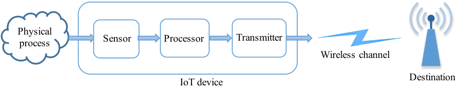
As illustrated in Fig. 1, we consider a time-critical IoT status updating system with a single IoT device and a destination.¹¹ 1 Although we consider only one device, the result in this paper can be extended to the IoT system with multiple devices by formulating the status updating problem as a restless multi-armed bandit (RMAB) problem. To solve the RMAB problem, Whittle’s index policy can be employed, where we decouple the problem with multiple devices into multiple sub-problems. There is only a single source-destination pair in each sub-problem, which is exactly the model we considered in this work. The IoT device is composed of a sensor which is capable of tracking the status of the underlying physical process, a processor which is capable of preprocessing the status update, and a transmitter which can deliver the status update over a wireless channel to the destination. The model with a single source-destination pair is simple but sufficient enough to investigate a wide range of applications. We assume that the IoT device adheres to the generate-at-will policy, which implies that a fresh status update is generated anytime an update decision is made.

Refer to caption — Figure 1: An illustration of the IoT status monitoring system.

A time-slotted system is considered, where time is divided into minislots with equal duration of $\tau$ (in seconds). In this system, a status update with $T_{u}$ packets is generated at the beginning of a minislot and at most one packet can be transmitted in one minislot. As such, the total duration for transmitting a single status update is $T_{u}$ minislots. The preprocessing at the IoT device could be data compression, feature extraction, or initial classification. In this work, we consider the preprocessing in general practice. Specifically, we characterize the preprocessing operation with three parameters, namely, the size of the status update before preprocessing $T_{u}$ , the size of the status update after preprocessing $T_{u}^{\prime}$ , and the number of CPU cycles per bit required to complete this operation $v$ .²² 2 Here, we would like to take the data compression as an example to explain the relationship between these parameters. For data compression, $T_{u}$ and $T_{u}^{\prime}$ are related to each other with a data compression ratio $\beta$ , i.e., $T_{u}^{\prime}=\beta T_{u}$ . Moreover, to perform the compression operation with the ratio $\beta$ , the number of CPU cycles required to compress one bit of the input data is $v$ . Let $l$ denote the number of bits per packet. Since the number of bit of the status update before processing is $T_{u}l$ , the number of minislots required for preprocessing one status update is then given by

T_{p}=\left\lceil\frac{T_{u}l\upsilon}{f\tau}\right\rceil,

(1)

where $f$ (in Hz) is the CPU frequency of the processor. We assume that the destination (e.g., a base station or an access point) has a more powerful computing capability. Therefore, the processing time at the destination is negligible compared to the processing time at the IoT device or the transmission time.

We refer to a decision epoch of the IoT device as a time step, as illustrated in Fig. 2. In each time step, the IoT device must determine whether to sample and transmit an update directly or preprocess the update before the transmission. Let $a_{p}(t)\in\{0,1\}$ denote the computing action at time step $t$ , where $a_{p}(t)=1$ indicates that the device preprocesses the status update, and $a_{p}(t)=0$ , otherwise. Let $a_{u}(t)\in\{0,1\}$ denote the updating action at time step $t$ , where $a_{u}(t)=1$ indicates that the device samples and transmits the status update to the destination and $a_{u}(t)=0$ , otherwise. Let $\boldsymbol{a}(t)\triangleq(a_{p}(t),a_{u}(t))\in\mathcal{A\triangleq}\left\{(0,0),(0,1),(1,1)\right\}$ denote the device’s control action vector at time step $t$ , where $\mathcal{A}$ is the feasible action space. In particular, if $\boldsymbol{a}(t)=(0,0)$ , the device will stay idle in one minislot. If $\boldsymbol{a}(t)=(0,1)$ , the device will sample and transmit the update directly without preprocessing. If $\boldsymbol{a}(t)=(1,1)$ , the device will first preprocess the status update after sampling and then transmit it to the destination. Notably, the action vector $(1,0)$ is not feasible because this action incurs energy consumption but does not provide the destination with a fresh status update.

It is important to emphasize that the duration of a time step is not uniform. Specifically, let $L(\boldsymbol{a}(t))$ denote the number of minislots in time step $t$ with action $\bm{a}(t)$ being taken, we can then express $L(\boldsymbol{a}(t))$ as follows

L(\boldsymbol{a}(t))=\begin{cases}1,&\text{if }\boldsymbol{a}(t)=(0,0),\\ T_{u},&\text{if }\boldsymbol{a}(t)=(0,1),\\ T_{p}+T_{u}^{\prime},&\text{if }\boldsymbol{a}(t)=(1,1).\end{cases}

(2)

We further denote by $L_{u}(\boldsymbol{a}(t))$ the transmission time corresponding to action $\bm{a}(t)$ , which is given as follows

L_{u}(\boldsymbol{a}(t))=\begin{cases}0,&\text{if }\boldsymbol{a}(t)=(0,0),\\ T_{u},&\text{if }\boldsymbol{a}(t)=(0,1),\\ T_{u}^{\prime},&\text{if }\boldsymbol{a}(t)=(1,1).\end{cases}

(3)

Let $C_{p}$ denote the computation energy consumption per minislot when $a_{p}(t)=1$ and $C_{u}$ denote the communication energy consumption per minislot when $a_{u}(t)=1$ . In particular, the computation energy consumption per minislot is given by

C_{p}=\kappa\tau f^{3},

(4)

where $\kappa$ is the effective switched capacitance depending on the chip architecture. By assuming a constant transmission power $P$ of the IoT device, the communication energy consumption per minislot is $C_{u}=P\tau$ . Then, the total energy consumption associated with action $\bm{a}(t)$ at time step $t$ is given by

\displaystyle C(\bm{a}(t))

\displaystyle=\begin{cases}0,&\text{if }\boldsymbol{a}(t)=(0,0),\\ T_{u}C_{u},&\text{if }\boldsymbol{a}(t)=(0,1),\\ T_{p}C_{p}+T_{u}^{\prime}C_{u},&\text{if }\boldsymbol{a}(t)=(1,1).\end{cases}

(5)

It is assumed that channel fading is constant in each minislot but varies independently across them. The channel state information is also assumed to be available only at the destination and the IoT device transmits an update at a fixed rate. We use a memoryless Bernoulli process $h(t,i)\in\{0,1\}$ to characterize the transmission failure because of outage, where $h(t,i)=1$ indicates that the packet is transmitted successfully at the $i$ -th minislot of time step $t$ , and $h(t,i)=0$ , otherwise. The transmission success probability of a packet is defined as

p_{s}=\Pr\{h(t,i)=1\}=\Pr\left\{B\log\left(1+\frac{\gamma P}{\sigma^{2}}\right)\geq\frac{l}{\tau}\right\},

(6)

where $B$ is the channel bandwidth, $\gamma$ is the channel gain between the IoT device and the destination, and $\sigma^{2}$ is the noise power. We assume that the status update can be successfully recovered at the destination if all the packets are transmitted successfully during one time step. We denote by $h(t)\in\{0,1\}$ the transmission status of an update at time step $t$ , i.e., $h(t)=\prod_{i=L(\boldsymbol{a}(t))-L_{u}(\boldsymbol{a}(t))+1}^{L(\boldsymbol{a}(t))}h(t,i)$ , where $h(t)=1$ indicates that the update is transmitted successfully, and $h(t)=0$ , otherwise. Thus, the transmission success probability of an update is given by $\Pr\{h(t)=1\}=p_{s}^{L_{u}(\boldsymbol{a}(t))}$ and the transmission failure probability of an update is given by $\Pr\{h(t)=0\}=1-p_{s}^{L_{u}(\boldsymbol{a}(t))}$ . We assume that there exists an instantaneous error-free single-bit ACK/NACK feedback from the destination to the IoT device. After a status update arrives at the destination, an ACK signal (a NACK signal) is sent in case of a successful reception (a failure).

The freshness of the status update is measured via AoI, which is defined as the time elapsed since the generation of the most recently received status update. Formally, let $U(t)$ denote the time step at which the most up-to-date status update successfully received by the destination was generated. Then, the AoI at the $i$ -th minislot of time step $t$ can be defined as

\displaystyle\delta(t,i)

\displaystyle=\mathrel{{\mathop{\sum}\limits}}L(\boldsymbol{a}(n))+i-1,

(7)

where the first term represents the number of minislots in the previous time steps since $U(t)$ and $i-1$ is the number of minislots in the current time step. For simplicity, we represent the AoI at the beginning of time step $t$ as $\delta(t)$ , i.e., $\delta(t)=\delta(t,1)=\sum_{n=U(t)}^{t-1}L(\boldsymbol{a}(n))$ .

Since it is pointless to receive a status update with a very large age for time-critical IoT application, we let $\hat{\delta}$ be the upper limit of the AoI, which is assumed to be finite but arbitrarily large [7]. Then, we present the dynamics of the AoI as follows

		$\displaystyle\delta(t+1)=$
		$\displaystyle\begin{cases}\min(\delta(t)+1,\hat{\delta}),&\text{if }\boldsymbol{a}(t)=(0,0),\\ \min(T_{u},\hat{\delta}),&\text{if }\boldsymbol{a}(t)=(0,1)\text{ and }h(t)=1,\\ \min(\delta(t)+T_{u},\hat{\delta}),&\text{if }\boldsymbol{a}(t)=(0,1)\text{ and }h(t)=0,\\ \min(T_{p}+T_{u}^{\prime},\hat{\delta}),&\text{if }\boldsymbol{a}(t)=(1,1)\text{ and }h(t)=1,\\ \min(\delta(t)+T_{p}+T_{u}^{\prime},\hat{\delta}),&\text{if }\boldsymbol{a}(t)=(1,1)\text{ and }h(t)=0.\end{cases}$		(8)

We also illustrate the AoI evolution process in Fig. 2.

Figure 2: An illustration of the evolution of the AoI, where

T_{u}=4

T_{u}^{\prime}=2

T_{p}=1

III Optimal Update Algorithm

III-A SMDP Formulation

Since the duration of each time step depends on the action taken in that time step, the time interval between two sequential actions is inconstant. Therefore, the optimal updating problem belongs to the class of SMDP. An SMDP can be defined as a tuple $(\mathcal{S},\mathcal{A},t^{+},\Pr(\cdot|\cdot),R)$ , where $\mathcal{S}$ is the state space, $\mathcal{A}$ is the action space, $t^{+}$ is the decision epoch, $\Pr(\cdot|\cdot)$ is the transition probability, and $r$ is the cost function. In particular, at the beginning of the time step $t$ , the agent observes the system state $s(t)$ and chooses an action $\bm{a}(t)$ . As a consequence, the system remains at $s(t)$ until the next decision epoch. Then, the system state transitions to $s(t+1)$ and the agent receives a cost $R(t)$ . We note that this is different from MDP, where the transition time is fixed and independent of the actions. In the following, we formally define the state, action, transition probability, and cost function of the SMDP.

III-A1 State

The state of the SMDP at time step $t$ $s(t)$ is defined to be the AoI at the beginning of that time step, i.e., $s(t)=\delta(t)$ . Since we limit the maximum value of the AoI, the state space is expressed as $\mathcal{S}\triangleq\{1,2,\cdots,\hat{\delta}\}$ .

III-A2 Action

The action at time step $t$ is $\boldsymbol{a}(t)$ and the action space is $\mathcal{A\triangleq}\left\{(0,0),(0,1),(1,1)\right\}$ .

III-A3 Decision Epoch

A decision is making at the beginning of a time step. The time interval between two adjacent decision epochs is $L(\bm{a}(t))$ , which depends on the action taking in time step $t$ .

III-A4 Transition Probability

We denote by $\Pr(s(t+1)\mid s(t),\boldsymbol{a}(t))$ the transition probability that a state transits from $s(t)$ to $s(t+1)$ with action $\boldsymbol{a}(t)$ . According to the AoI evolution dynamic in (8), the transition probability can be given as follows

\displaystyle\begin{cases}\Pr\left(\min(\delta(t)+1,\hat{\delta})\mid\delta(t),(0,0)\right)=1,\\ \Pr\left(\min(T_{u},\hat{\delta})\mid\delta(t),(0,1)\right)=p_{s}^{T_{u}},\\ \Pr\left(\min(\delta(t)+T_{u},\hat{\delta})\mid\delta(t),(0,1)\right)=1-p_{s}^{T_{u}},\\ \Pr\left(\min(T_{p}+T_{u}^{\prime},\hat{\delta})\mid\delta(t),(1,1)\right)=p_{s}^{T_{u}^{\prime}},\\ \Pr\left(\min(\delta(t)+T_{p}+T_{u}^{\prime},\hat{\delta})\mid\delta(t),(1,1)\right)=1-p_{s}^{T_{u}^{\prime}}.\end{cases}

(9)

III-A5 Cost

We aim to minimize the weighted sum of the average AoI associated with the destination and the energy consumed by the IoT device. As such, we define the cost at a time step as the weighted sum of the AoI and the energy consumption. Specifically, the cost at time step $t$ is represented as

	$\displaystyle R(\delta(t),\boldsymbol{a}(t))$
$\displaystyle=$	$\displaystyle\mathrel{{\mathop{\sum}\limits}}\delta(t,i)+\omega C(\bm{a}(t))$
$\displaystyle=$	$\displaystyle\mathrel{{\mathop{\sum}\limits}}(\delta(t)+i-1)+\omega C(\bm{a}(t))$
$\displaystyle=$	$\displaystyle\frac{1}{2}(2\delta(t)+L(\boldsymbol{a}(t))-1)L(\boldsymbol{a}(t))+\omega C(\bm{a}(t)),$	(10)

where $\omega$ is the weighting factor.

Our goal is to find an update policy $\pi=(\boldsymbol{a}(1),\boldsymbol{a}(2),\ldots)$ that reduces the average cost to the lowest possible level. Under a set of stationary deterministic policy $\Pi$ and a given initial system state $s(1)$ , the objective can be formulated as follows:

\displaystyle\min_{\pi\in\Pi}\limsup_{T\rightarrow\infty}\frac{\mathbb{E}\left[\mathrel{{\mathop{\sum}\limits}}R(\delta(t),\boldsymbol{a}(t))\mid s(1)\right]}{\mathbb{E}\left[\mathrel{{\mathop{\sum}\limits}}L(\boldsymbol{a}(t))\right]}.

(11)

Since the duration of the time step is not uniform, the average cost in (11) is defined as the limit of the expected total cost over a finite number of time steps divided by the expected cumulative time of these time steps [5]. In this work, we restrict our attention to stationary unichain policy, under which the Markov chain is composed of a single recurrent class and a set of transient states. Thus, the average cost is independent on the initial state and the Markov chain has a unique stationary distribution [15].

To solve this problem, we transform the SMDP into an equivalent discrete time MDP using uniformization [16, 15]. Let $\mathcal{\bar{S}}$ and $\mathcal{\bar{A}}$ denote the state space and action space of the transformed MDP. They are the same as those in the original SMDP, i.e., $\mathcal{\bar{S}}=\mathcal{S}$ and $\mathcal{\bar{A}}=\mathcal{A}$ . For any $s\in\bar{\mathcal{S}}$ and $\boldsymbol{a}\in\bar{\mathcal{A}}$ , the cost in the MDP is given by

\bar{R}(s,\boldsymbol{a})=\frac{R(s,\boldsymbol{a})}{L(\boldsymbol{a})}=s+\frac{1}{2}(L(\boldsymbol{a})-1)+\omega\frac{C(\bm{a})}{L(\boldsymbol{a})},

(12)

and the transition probability is given by

\bar{p}(s^{\prime}\mid s,\boldsymbol{a})=\begin{cases}\frac{\epsilon}{L(\boldsymbol{a})}p(s^{\prime}\mid s,\boldsymbol{a}),&s^{\prime}\neq s,\\ 1-\frac{\epsilon}{L(\boldsymbol{a})},&s^{\prime}=s,\end{cases}

(13)

where $\epsilon$ is chosen in $\Big(0,\min\limits_{\boldsymbol{a}}L(\boldsymbol{a})\Big]$ .

Then, by solving the Bellman equation in (14), one can obtain the optimal policy $\pi^{*}$ of the original SMDP that minimizes the average cost. According to [16], we have

\theta+V(s)=\min\limits_{\boldsymbol{a}\in\mathcal{A}}\bigg\{\bar{R}(s,\boldsymbol{a})+\sum\limits_{s^{\prime}\in\mathcal{S}}\bar{p}(s^{\prime}\mid s,\boldsymbol{a})V(s^{\prime})\bigg\},\forall s\in\mathcal{S},

(14)

where $\theta$ is the optimal value to (11) for all initial state and $V(s)$ is the value function for the discrete-time MDP. Then, the optimal policy can be given by

\pi^{*}(s)=\arg\min\limits_{\boldsymbol{a}\in\mathcal{A}}\bigg\{\bar{R}(s,\boldsymbol{a})+\sum\limits_{s^{\prime}\in\mathcal{S}}\bar{p}(s^{\prime}\mid s,\boldsymbol{a})V(s^{\prime})\bigg\}

(15)

for any $s\in\mathcal{S}$ . Theoretically, we can obtain the optimal policy $\pi^{*}$ via (15). However, the value function $V(\cdot)$ does not have closed-form solution in general, which makes this problem challenging. Although numerical algorithms such as value iteration and policy iteration can solve this problem, they incur high computational complexity and do not provide many design insights. For a better understanding of the system, we will investigate the structural properties of the optimal update policy in the next subsection.

III-B Structural Analysis and Algorithm Design

In this subsection, we first show that the structure of the optimal policy is of threshold-type with respect to the AoI. Then, we propose a relative policy iteration algorithm based on the threshold structure to obtain the optimal policy $\pi^{*}$ for (11).

To begin with, we show some key properties of the value function $V(s)$ in the following lemmas.

Lemma 1.

The value function $V(s)$ is non-decreasing with $s$ .

Proof:

See Appendix -A. ∎

Lemma 2.

The value function $V(s)$ is concave in $s$ .

Proof:

See Appendix -B. ∎Since $V(s)$ is a concave function, its slope is non-increasing. We drive the lower bound of the slope of $V(s)$ in the following lemma. Before that, we define an auxiliary variable $\bm{a}_{f}$ , which is given by

\boldsymbol{a}_{f}=\begin{cases}(0,1),&\frac{T_{u}}{p_{s}^{T_{u}}}\leq\frac{T_{p}+T_{u}^{\prime}}{p_{s}^{T_{u}^{\prime}}},\\ (1,1),&\frac{T_{u}}{p_{s}^{T_{u}}}\geq\frac{T_{p}+T_{u}^{\prime}}{p_{s}^{T_{u}^{\prime}}}.\end{cases}

(16)

Lemma 3.

For any $s_{1},s_{2}\in\mathcal{S}$ , such that $s_{1}\leq s_{2}$ , $V(s_{2})-V(s_{1})\geq\frac{L(\boldsymbol{a}_{f})}{\epsilon p_{s}^{L_{u}(\boldsymbol{a}_{f})}}(s_{2}-s_{1})$ .

Proof:

See Appendix -C. ∎We are now in position to show the structure of the optimal update policy.

Theorem 1.

For any $s_{1},s_{2}\in\mathcal{S}$ , such that $s_{1}\leq s_{2}$ , there is an optimal policy that satisfies the structural properties as follow:

A) When $\frac{T_{u}}{p_{s}^{T_{u}}}\leq\frac{T_{p}+T_{u}^{\prime}}{p_{s}^{T_{u}^{\prime}}}$ , if $\pi^{*}(s_{1})=(0,1)$ , then $\pi^{*}(s_{2})=(0,1)$ .

B) When $\frac{T_{u}}{p_{s}^{T_{u}}}\geq\frac{T_{p}+T_{u}^{\prime}}{p_{s}^{T_{u}^{\prime}}}$ , if $\pi^{*}(s_{1})=(1,1)$ , then $\pi^{*}(s_{2})=(1,1)$ .

Proof:

See Appendix -D. ∎Theorem 1 depicts the structural properties of the optimal policy $\pi^{*}$ of the SMDP in two cases. We note that $\frac{T_{u}}{p_{s}^{T_{u}}}$ and $\frac{T_{p}+T_{u}^{\prime}}{p_{s}^{T_{u}^{\prime}}}$ can be interpreted as the expected duration of repeatedly taking action $(0,1)$ and that of taking action $(1,1)$ to get one success transmission, respectively. Therefore, Theorem 1 also suggests when to choose which updating action in the high AoI regime. Particularly, in order to minimize the long-term average cost, the updating action with a shorter expected duration should be chosen when the AoI is large enough to dominate the cost. For example, in the first case where the preprocessing incurs a larger expected update duration, it is better to transmit the update directly for a large enough AoI, while in the second case where preprocessing can help shorten the expected update duration, it is no doubt to choose preprocessing-and-transmission when the AoI is large enough. The reason why we do not consider the energy consumption of both actions in the conditions is that the difference between the energy consumption of different actions is constant and the age increasingly dominates the cost as the AoI grows larger. We further illustrate the threshold structure of the optimal policy in Fig. 3, where the structure of optimal policy falls into case 1 when $v\leq 10$ , and otherwise when $v\geq 12$ .

Figure 3: Structure of the optimal policy for different values of

v

(

T_{u}=4

T_{u}^{\prime}=2

l=3

f=35

\tau=1

\kappa=0.00005

P=6

\omega=2

p_{s}=0.8

Remark 1.

We note that the result in Theorem 1 can be extended to the case of discrete transmit power control. The action with the largest transmit power would be the optimal one when the AoI is large enough, because the largest transmit power can bring the shortest expected duration.

According to Theorem 1, there exists a threshold $\Omega$ in the optimal update policy. Although the exact values of $\Omega$ depend on the particular values of $V(s)$ , the structure only depends on the properties of $V(s)$ . Therefore, a low-complexity relative policy iteration algorithm can be developed by incorporating the threshold structure into a standard relative policy iteration algorithm. In particular, we will no longer need to minimize the righthand side of (14) for all states to find $\pi^{*}$ , thereby reducing the computational complexity. The details are given in Algorithm 1.

Algorithm 1 Relative Policy Iteration based on the Threshold Structure

1: Initialization: Set

\pi_{0}^{*}(s)=(0,0)

for all

s\in\mathcal{S}

, select a reference state

s^{\dagger}

, and set

k=0

2: Policy Evaluation: Given

\pi_{k}^{*}

, compute the value of

\theta_{k}

and

V_{k}(s)

from the linear system of equations

\begin{cases}\begin{aligned} \theta_{k}+V_{k}(s)=&\bar{R}(s,\pi_{k}^{*}(s))\\ &+\sum\limits_{s^{\prime}\in\mathcal{S}}\bar{p}(s^{\prime}\mid s,\pi_{k}^{*}(s))V_{k}(s^{\prime}),\end{aligned}\\ V_{k}(s^{\dagger})=0,\end{cases}

(17)

by Gaussian elimination.

3: Structured Policy Improvement: Compute a new policy

\pi_{k+1}^{*}

for each

s\in\mathcal{S}

as follows: if

\frac{T_{u}}{p_{s}^{T_{u}}}\leq\frac{T_{p}+T_{u}^{\prime}}{p_{s}^{T_{u}^{\prime}}}

and

\pi_{k+1}^{*}(s-1)=(0,1),

then

\pi_{k+1}^{*}(s)=(0,1).

else if

\frac{T_{u}}{p_{s}^{T_{u}}}\geq\frac{T_{p}+T_{u}^{\prime}}{p_{s}^{T_{u}^{\prime}}}

and

\pi_{k+1}^{*}(s-1)=(1,1),

then

\pi_{k+1}^{*}(s)=(1,1).

else

	$\displaystyle\pi_{k+1}^{*}(s)=\arg\min_{\boldsymbol{a}\in\mathcal{A}}$	$\displaystyle\{\bar{R}(s,\pi_{k}^{*}(s))$
		$\displaystyle+\sum\limits_{s^{\prime}\in\mathcal{S}}\bar{p}(s^{\prime}\mid s,\pi_{k}^{*}(s))V_{k}(s^{\prime})\}.$		(18)

4: Set

k=k+1

and go to Step 2 until

\pi_{k}^{*}(s)=\pi_{k+1}^{*}(s)

for all

s\in\mathcal{S}

IV Special Case Study: Transmission over a Reliable Channel

In this section, we consider a special scenario where the packets are transmitted over a reliable channel. Accordingly, the status updating problem can be simplified. From (8) we can see that the states smaller than $\min\{T_{u},T_{p}+T_{u}^{\prime}\}$ are non-recurrent states. Since the policies in non-recurrent states has no effect on the average cost, we can only consider the state space $\mathcal{S}^{\dagger}\triangleq\left\{\min\{T_{u},T_{p}+T_{u}^{\prime}\},\cdots,\hat{\delta}\right\}$ when discussing the optimal policy.

IV-A Case 1

Based on the model of the reliable channel, we give the first simplification of the optimal policy.

Lemma 4.

For any $s\in\mathcal{S}^{\dagger}$ , we have $\pi^{*}(s)\neq(0,0)$ when $\frac{1}{2}L(\boldsymbol{a}_{f})(L(\boldsymbol{a}_{f})+1)\geq\omega C(\boldsymbol{a}_{f})$ .

Proof:

See Appendix -E. ∎Lemma 4 indicates that the IoT device will never stay idle with the optimal policy when the AoI dominates in the cost. Accordingly, the threshold structure in Theorem 1 can be simplified, which is presented in the theorem below.

Theorem 2.

For $s\in\mathcal{S}^{\dagger}$ , the optimal policy is of a switch-type structure when $\frac{1}{2}L(\boldsymbol{a}_{f})(L(\boldsymbol{a}_{f})+1)\geq\omega C(\boldsymbol{a}_{f})$ , namely, there exists a threshold $\Omega\geq\min\{T_{u},T_{p}+T_{u}^{\prime}\}$ , such that when $T_{u}\leq T_{p}+T_{u}^{\prime}$ ,

\pi^{*}(s)=\begin{cases}(1,1),&T_{u}\leq s<\Omega,\\ (0,1),&s\geq\Omega,\end{cases}

(19)

and when $T_{u}\geq T_{p}+T_{u}^{\prime}$ ,

\pi^{*}(s)=\begin{cases}(0,1),&T_{p}+T_{u}^{\prime}\leq s<\Omega,\\ (1,1),&s\geq\Omega.\end{cases}

(20)

Proof:

According to Lemma 4, we can exclude action $(0,0)$ from the optimal policy when $\frac{1}{2}L(\boldsymbol{a}_{f})(L(\boldsymbol{a}_{f})+1)\geq\omega C(\boldsymbol{a}_{f})$ . Moreover, since we have proved the threshold structure of the optimal policy in a general case in Theorem 1, the optimal policy can be further proved to satisfy the switching structure in (19) and (20). ∎Theorem 2 depicts the structure of the optimal policy $\pi^{*}$ for the SMDP in (11) when $p_{s}=1$ and $\frac{1}{2}L(\boldsymbol{a}_{f})(L(\boldsymbol{a}_{f})+1)\geq\omega C(\boldsymbol{a}_{f})$ . We further illustrate the analytical results of Theorem 2 in Fig. 4, where $T_{u}\leq T_{p}+T_{u}^{\prime}$ and $C(\bm{a}=(0,1))>C(\bm{a}=(1,1))$ . It can be seen from Fig. 4 that the optimal policy is of the threshold type. Moreover, the threshold increases along with $\omega$ . This indicates that, when the weighting factor is large, it is not desirable to directly transmit a new status update to the destination due to a high weighted energy consumption.

Figure 4: Structure of the optimal policy in Theorem 2 for different values of

\omega

(

T_{u}=5

T_{u}^{\prime}=1

l=3

v=5

f=15

\tau=1

\kappa=0.00005

P=3

We then denote $\boldsymbol{a}_{1}=\arg\min\limits_{\boldsymbol{a}\in\mathcal{A}\setminus(0,0)}\{L(\boldsymbol{a})\}$ and $\boldsymbol{a}_{2}=\arg\max\limits_{\boldsymbol{a}\in\mathcal{A}\setminus(0,0)}\{L(\boldsymbol{a})\}$ . According to the threshold structure in Theorem 2, we can proceed to reduce the recurrent state space of the computing-enable IoT system.

Lemma 5.

For a given threshold policy of the type in Theorem 2 with the threshold of $\Omega$ , recurrent state space $\mathcal{S}^{\prime}$ can be given as follow:

A) $\mathcal{S}^{\prime}=\left\{L(\boldsymbol{a}_{1})\right\}$ when $\Omega=L(\boldsymbol{a}_{1})$ .

B) $\mathcal{S}^{\prime}=\left\{L(\boldsymbol{a}_{1}),L(\boldsymbol{a}_{2})\right\}$ when $L(\boldsymbol{a}_{1})<\Omega\leq L(\boldsymbol{a}_{2})$ .

C) $\mathcal{S}^{\prime}=\left\{L(\boldsymbol{a}_{2})\right\}$ when $\Omega>L(\boldsymbol{a}_{2})$ .

Proof:

As illustrated in Fig. 5, we can use a Discrete Time Markov Chain (DTMC) to model the MDP constructed by any threshold policy of the type in Theorem 2 with the threshold of $\Omega$ . It can be seen from Fig. 5(a) and Fig. 5(c), respectively, that there is only one recurrent state $L(\boldsymbol{a}_{1})$ when $\Omega=L(\boldsymbol{a}_{1})$ and $L(\boldsymbol{a}_{2})$ when $\Omega>L(\boldsymbol{a}_{2})$ . Also we can see from Fig. 5(b) that the recurrent states are $L(\boldsymbol{a}_{1})$ and $L(\boldsymbol{a}_{2})$ when $L(\boldsymbol{a}_{1})<\Omega\leq L(\boldsymbol{a}_{2})$ . ∎

(a)

(b)

(c)

Figure 5: The states transitions under a threshold policy with different values of

\Omega

. (a)

\Omega=L(\boldsymbol{a}_{1})

. (b)

L(\boldsymbol{a}_{1})<\Omega\leq L(\boldsymbol{a}_{2})

. (c)

\Omega>L(\boldsymbol{a}_{2})

Under the threshold policy, we proceed with analyzing the average cost of any threshold $\Omega$ .

Lemma 6.

Let $J_{1}=\frac{3}{2}L(\boldsymbol{a}_{1})+\omega\frac{C(\boldsymbol{a}_{1})}{L(\boldsymbol{a}_{1})}-\frac{1}{2}$ , $J_{2}=L(\boldsymbol{a}_{1})L(\boldsymbol{a}_{2})+\omega\frac{C(\boldsymbol{a}_{1})+C(\boldsymbol{a}_{2})}{L(\boldsymbol{a}_{1})+L(\boldsymbol{a}_{2})}$ , $J_{3}=\frac{3}{2}L(\boldsymbol{a}_{2})+\omega\frac{C(\boldsymbol{a}_{2})}{L(\boldsymbol{a}_{2})}-\frac{1}{2}$ . For a given threshold $\Omega$ , the average cost of the threshold policy in Theorem 2 is given by

J(\Omega)=\begin{cases}J_{1},&\Omega=L(\boldsymbol{a}_{1}),\\ J_{2},&L(\boldsymbol{a}_{1})<\Omega\leq L(\boldsymbol{a}_{2}),\\ J_{3},&\Omega>L(\boldsymbol{a}_{2}).\end{cases}

(21)

Proof:

See Appendix -F. ∎By leveraging the above results, we can find the set of the optimal threshold $\Omega^{*}$ .

Theorem 3.

If $J_{1}$ is smaller than $J_{2}$ and $J_{3}$ , we have $\Omega^{*}=L(\boldsymbol{a}_{1})$ . If $J_{2}$ is smaller than $J_{1}$ and $J_{3}$ , we have $L(\boldsymbol{a}_{1})<\Omega^{*}\leq L(\boldsymbol{a}_{2})$ . If $J_{3}$ is smaller than $J_{1}$ and $J_{2}$ , we have $\Omega^{*}>L(\boldsymbol{a}_{2})$ .

Proof:

According to Lemma 6, we can determine the set of the optimal threshold $\Omega^{*}$ by comparing the values of $J_{1}$ , $J_{2}$ and $J_{3}$ . ∎We have proved in Lemma 5 that under the threshold policy in Theorem 2, only a few states of the system are recurrent states. Once the set of the optimal threshold is determined, we can determine the optimal policy in the recurrent states. Therefore, the specific value of the threshold is not a necessity. As long as we take any value in the set of the optimal threshold, we can achieve the goal of minimizing the average cost.

IV-B Case 2

Based on the model of the reliable channel, we give the second simplification of the optimal policy. Recall that $\boldsymbol{a}_{1}=\arg\min\limits_{\boldsymbol{a}\in\mathcal{A}\setminus(0,0)}\{L(\boldsymbol{a})\}$ and $\boldsymbol{a}_{2}=\arg\max\limits_{\boldsymbol{a}\in\mathcal{A}\setminus(0,0)}\{L(\boldsymbol{a})\}$ , we have the following lemma.

Lemma 7.

For any $s\in\mathcal{S}^{\dagger}$ , we have $\pi^{*}(s)\neq\boldsymbol{a}_{2}$ when $\frac{C(\boldsymbol{a}_{1})}{L(\boldsymbol{a}_{1})}\leq\frac{C(\boldsymbol{a}_{2})}{L(\boldsymbol{a}_{2})}$ .

Proof:

See Appendix -G. ∎Lemma 7 reveals that the action with a lower energy efficiency (i.e., a larger energy consumption per minislot) shall be excluded in the optimal policy. Accordingly, the threshold structure in Theorem 1 is simplified in the following theorem.

Theorem 4.

For $s\in\mathcal{S}^{\dagger}$ , the optimal policy is of a switch-type structure when $\frac{C(\boldsymbol{a}_{1})}{L(\boldsymbol{a}_{1})}\leq\frac{C(\boldsymbol{a}_{2})}{L(\boldsymbol{a}_{2})}$ , namely, there is a threshold $\Omega\geq\min\{T_{u},T_{p}+T_{u}^{\prime}\}$ , such that

\pi^{*}(s)=\begin{cases}(0,0),&L(\boldsymbol{a}_{1})\leq s<\Omega,\\ \boldsymbol{a}_{1},&s\geq\Omega.\end{cases}

(22)

Proof:

According to Lemma 7, we can exclude $\bm{a}_{2}$ from the optimal policy when $\frac{C(\boldsymbol{a}_{1})}{L(\boldsymbol{a}_{1})}\leq\frac{C(\boldsymbol{a}_{2})}{L(\boldsymbol{a}_{2})}$ . Moreover, since we have proved the threshold structure of the optimal policy in a general case in Theorem 1, the optimal policy can be further proved to satisfy the switching structure in (22). ∎Theorem 4 depicts the structure of the optimal policy $\pi^{*}$ for the SMDP in (11) when $p_{s}=1$ and $\frac{C(\boldsymbol{a}_{1})}{L(\boldsymbol{a}_{1})}\leq\frac{C(\boldsymbol{a}_{2})}{L(\boldsymbol{a}_{2})}$ . Fig. 6 illustrates the analytical results of Theorem 4, where $p_{s}=1$ and $C_{u}\geq\frac{T_{p}C_{p}+T_{u}^{\prime}C_{u}}{T_{p}+T_{u}^{\prime}}$ . We can see from Fig. 6 that, in order to strike a balance between the AoI and the energy consumption, the IoT device does not transmit until the AoI is large. We can also see that the threshold increases with the increasing of the weighting factor $\omega$ . This is due to a higher weighted energy consumption in average cost when $\omega$ grows larger.

Figure 6: Structure of the optimal policy in Theorem 4 for different values of

\omega

(

T_{u}=6

T_{u}^{\prime}=2

l=3

v=5

f=45

\tau=1

\kappa=0.00005

P=6

Under the threshold policy in Theorem 4, we proceed with analyzing the average cost.

Lemma 8.

The average cost of the threshold policy for any given threshold $\Omega$ in Theorem 4 can be given by

J(\Omega)=L(\boldsymbol{a}_{1})+\frac{1}{2}(\Omega-1)+\frac{\omega C(\bm{a}_{1})}{\Omega}.

(23)

Proof:

See Appendix -H. ∎By leveraging the above results, we can find the optimal threshold value $\Omega^{*}$ .

Theorem 5.

The optimal threshold $\Omega^{*}$ of the optimal update policy in Theorem 4 is given by

\Omega^{*}=\arg\min\left(J\left(\left\lfloor\sqrt{2\omega C(\bm{a}_{1})}\right\rfloor\right),J\left(\left\lceil\sqrt{2\omega C(\bm{a}_{1})}\right\rceil\right)\right).

(24)

Proof:

See Appendix -I. ∎From the expression of the optimal threshold $\Omega^{*}$ , we can see that the threshold is monotonically increasing with respect to $\omega$ and $C(\boldsymbol{a}_{1})$ , which is consistent with the result in Fig. 6. This indicates that, when the weighting factor or the energy consumption is large, transmitting a new status update can achieve better result than keeping idle only in the large AoI regime.

Remark 2.

In this section, by studying the special cases, we show that the optimal policy has a switching structure with respect to only two actions. Moreover, the optimal threshold can be obtained in closed-form, which reveals how the system parameters affect the threshold policy. It is worth noting that, in practice, the conclusions obtained from the special cases study can be applied in the high SNR regime and the obtained optimal policy can be used as an approximation of the optimal policy when the success rate is high.

V Simulation Results

In this section, we present the simulation results to explore the effects of system parameters on the optimal update policy and demonstrate the efficacy of the proposed scheme by comparing it with two other zero-wait policies, i.e., zero-wait no-computation policy and zero-wait computation policy. Particularly, in both baseline policies, the IoT device starts a new transmission immediately after the previous transmission is finished. In the zero-wait no-computation policy, the IoT device transmits each status update without preprocessing, while, in the zero-wait computation policy, the IoT device preprocesses each status update and then transmits the processed status update. In the simulations, we truncate the state space by setting the upper limit of the number of states to be 200.

V-A Performance Evaluation in the General Case

(a)

(b)

Figure 7: Performance comparison among the optimal policy, the zero-wait no-computation policy, and the zero-wait computation policy (

T_{u}=4

T_{u}^{\prime}=2

l=3

v=2

f=35

\tau=1

\kappa=0.00005

P=6

\omega=2

). (a) The average cost versus

p_{s}

. (b) The average AoI and the average energy consumption versus

p_{s}

In Fig. 7, the average cost of the optimal policy and the two baseline policies are compared with respect to the transmission success probability $p_{s}$ . As we can see from Fig. 7(a), the optimal policy outperforms the zero-wait policies. Moreover, the average cost decreases as $p_{s}$ increases. The reason can be explained with the aid of Fig 7(b). First, it is evident that the average AoI of all the three policies decreases with the increasing of $p_{s}$ since the AoI is more likely to be reset with a larger transmission success probability. Second, because the IoT device with zero-wait policies keep updating continuously, the average energy consumption remains a constant irrespective of $p_{s}$ . For $0.1\leq p_{s}\leq 1$ , we can see that the average energy consumption steadily decreases with the increase of $p_{s}$ . This is due to the fact that less transmission is needed to reduce the AoI when $p_{s}$ is larger. Therefore, the optimal policy can adapt to the channel quality. Through this comparison, we can see that although the optimal update policy does not yield the minimum AoI, it has a smaller energy consumption than the zero-wait policies. By trading off the AoI for energy consumption, the optimal update policy achieves the smallest average cost.

(a)

(b)

Figure 8: Performance comparison among the optimal policy, the zero-wait no-computation policy, and the zero-wait computation policy (

T_{u}=4

T_{u}^{\prime}=2

l=3

f=35

\tau=1

\kappa=0.00005

P=6

\omega=2

p_{s}=0.8

). (a) The average cost versus

v

. (b) The average AoI and the average energy consumption versus

v

In Fig. 8, the average cost of the optimal policy and the two baseline policies are compared with respect to the number of CPU cycles required to preprocess one bit $v$ . We can see from Fig. 8(a) that the optimal policy outperforms both baseline policies. It is easy to see that the performance of zero-wait no-computation policy is irrespective of $v$ since each status update is transmitted directly without preprocessing. In contrast, the average cost of the optimal policy and the zero-wait computation policy is non-decreasing as $v$ grows. Particularly, we can see from Fig. 8(b) that the average AoI of the zero-wait computation policy increases with $v$ . Since the status update is more and more computation intensive as $v$ grows, the preprocessing at the IoT device requires more and more time, which leads to an increase in the average AoI. However, since the computation energy consumption per minislot in this setup is less than the transmission energy consumption per minislot, the average energy consumption of the zero-wait computation policy is shown to decline with $v$ . In other words, although the duration and total energy consumption are increasing as $v$ increases, the average energy consumption is decreasing. Moreover, we can see from Fig. 8(b) that the average AoI of the optimal update policy is non-decreasing with $v$ except when $14\leq v\leq 16$ . The reason why the average AoI of the optimal policy drops for $14\leq v\leq 16$ can be explained with Fig. 3. Since $v=16$ , the optimal policy completely abandons the action of $(1,1)$ . The change of the optimal policy effectively reduces the average AoI of the system, but induces a sudden increase in the average energy consumption at $v=16$ . We can also see that the average energy consumption increases as $v$ increases. This is because the optimal policy makes sacrifices in energy consumption in order to ensure that the AoI is increased at a slower pace. It could be concluded that the optimal update policy can adjust adaptively based on the degree of computational intensity of the status update.

V-B Performance Evaluation in the Special Cases

In this subsection, we show the performance of two different special cases in Section IV that the packets are transmitted over a reliable channel. In Fig. 9, the average cost of the optimal policy and the two baseline policies are compared with respect to the weighting factor $\omega$ when $T_{u}\leq T_{p}+T_{u}^{\prime}$ and $\frac{1}{2}(T_{p}+T_{u}^{\prime})(T_{p}+T_{u}^{\prime}+1)\geq\omega(T_{p}C_{p}+T_{u}^{\prime}C_{u})$ . As we can see from Fig. 9(a), the optimal policy outperforms both two baseline policies. Moreover, the optimal policy coincides with the zero-wait no-computation policy when $\omega$ is small and coincides with the zero-wait computation policy when $\omega$ is large. This is because, in this simulation setup, when $w\leq 0.55$ , we have $\min(J_{1},J_{2},J_{3})=J_{1}$ and the optimal policy is to always transmit the status update directly, while when $w\geq 0.75$ , we have $\min(J_{1},J_{2},J_{3})=J_{3}$ and the optimal policy is to always preprocess and transmit the status update. Moreover, when $0.60\leq w\leq 0.70$ , we have $\min(J_{1},J_{2},J_{3})=J_{2}$ and the optimal policy is to execute the above two actions in turns. That is the reason why the optimal policy outperforms the two zero-wait policies in this regime.

(a)

(b)

Figure 9: Performance comparison among the optimal policy, the zero-wait no-computation policy, and the zero-wait computation policy (

T_{u}=5

T_{u}^{\prime}=1

l=3

v=5

f=15

\tau=1

\kappa=0.00005

P=3

). (a) The average cost versus

\omega

. (b) The average AoI and the average energy consumption versus

\omega

In Fig. 10, the average cost of the optimal policy and the two baseline policies are compared with respect to $\omega$ when $T_{u}\geq T_{p}+T_{u}^{\prime}$ and $C_{u}\geq\frac{T_{p}C_{p}+T_{u}^{\prime}C_{u}}{T_{p}+T_{u}^{\prime}}$ . As we can see from Fig. 10(a), the optimal policy outperforms both two baseline policies. As the weight factor increases, the average cost of the optimal policy and the baseline policies increase but with different rates. From Fig. 10(b) we can see that the average AoI and the energy consumption of the two zero-wait baseline policies are constant for any $\omega$ . The gap between the optimal policy and the zero-wait baseline policies grows with $\omega$ in 10(a), because the zero-wait policies suffer from a higher weighted energy consumption when the weighting factor is large. For the optimal policy, we can see that, with the increase of $\omega$ , its average energy consumption tends to be smaller while the average AoI tends to be larger. This is the result of the balance between the AoI reduction and the energy consumption. Theorem 8 shows that the threshold of the optimal policy in this case will increase with $\omega$ . Therefore, when $\omega$ is large, the IoT device will update only when the AoI is large enough.

(a)

(b)

Figure 10: Performance comparison among the optimal policy, the zero-wait no-computation policy, and the zero-wait computation policy (

T_{u}=6

T_{u}^{\prime}=2

l=3

v=5

f=45

\tau=1

\kappa=0.00005

P=6

). (a) The average cost versus

\omega

. (b) The average AoI and the average energy consumption versus

\omega

VI Conclusion

In this paper, we have studied the problem for optimizing information freshness in computing-enabled IoT systems by jointly controlling the preprocessing and transmission at the IoT device. To minimize the weighted sum of the average AoI associated with the destination and the energy consumed by the IoT device, we have formulated an infinite horizon average cost SMDP. By transforming the SMDP to an equivalent uniform time step MDP, we have investigated the structure of the optimal update policy and provided a structure-aware relative policy iteration algorithm. We have further proved the switch-type structure of the optimal policy in a special scenario where the status updates are transmitted over a reliable channel. Simulation results have shown that the optimal update policy can adjust adaptively based on the channel quality and the degree of computational intensity of the status update. By comparing the optimal update policy with two other zero-wait policies, it is shown that the optimal update policy achieves a good balance between the AoI reduction and the energy consumption.

-A Proof of Lemma 1

According to the value iteration algorithm (VIA) [17, Chapter 4.3], we prove Lemma 1 by using mathematical induction. We first denote by $V_{k}(s)$ and $Q_{k}(s,\bm{a})$ the state value function and state-action value functions at iteration $k$ , respectively. In particular, $Q_{k}(s,\bm{a})$ is defined as:

Q_{k}(s,\boldsymbol{a})\triangleq\bar{R}(s,\boldsymbol{a})+\sum\limits_{s^{\prime}\in\mathcal{S}}\bar{p}(s^{\prime}\mid s,\boldsymbol{a})V_{k}(s^{\prime}),\forall s\in\mathcal{S},

(25)

where $s^{\prime}$ is given by (8). For each state $s$ , VIA calculates $V_{k+1}(s)$ according to

V_{k+1}(s)=\min\limits_{\boldsymbol{a}\in\mathcal{A}}Q_{k}(s,\boldsymbol{a}).

(26)

Under any initialization of $V_{0}(s)$ , the generated sequence $\{V_{k}(s)\}$ converges to $V(s)$ , i.e.,

\lim_{k\rightarrow\infty}V_{k}(s)=V(s),\forall s\in\mathcal{S},

(27)

where $V(s)$ satisfies the Bellman equation in (14). Therefore, we can prove the monotonicity of $V(s)$ by showing that this property is also possessed by $V_{k}(s)$ for any $k$ . Particularly, we need to prove that for any $s_{1},s_{2}\in\mathcal{S}$ , such that $s_{1}\leq s_{2}$ ,

V_{k}(s_{1})\leq V_{k}(s_{2}),\quad k=0,1,\ldots

(28)

We initialize $V_{0}(s)=0$ for all $s\in\mathcal{S}$ without sacrificing generality. Then, we prove (28) by using mathematical induction. First, since $V_{0}(s)=0$ for all $s\in\mathcal{S}$ , (28) holds for $k=0$ . Next, we assume that (28) holds up till $k>0$ and inspect whether it holds for $k+1$ .

When $\boldsymbol{a}=(0,0)$ , we have $Q_{k}(s_{1},(0,0))=s_{1}+(1-\epsilon)V_{k}(s_{1})+\epsilon V_{k}(s_{1}+1)$ and $Q_{k}(s_{2},(0,0))=s_{2}+(1-\epsilon)V_{k}(s_{2})+\epsilon V_{k}(s_{2}+1)$ . Since $s_{1}\leq s_{2}$ , $V_{k}(s_{1})\leq V_{k}(s_{2})$ and $V_{k}(s_{1}+1)\leq V_{k}(s_{2}+1)$ , we can easily see that $Q_{k}(s_{1},(0,0))\leq Q_{k}(s_{2},(0,0))$ .

When $\boldsymbol{a}=(0,1)$ or $(1,1)$ , the state-action value functions at iteration $k$ are given by

$\displaystyle Q_{k}(s_{1},\boldsymbol{a})$	$\displaystyle=s_{1}+\frac{1}{2}(L(\boldsymbol{a})-1)+\omega\frac{C(\boldsymbol{a})}{L(\boldsymbol{a})}$
	$\displaystyle+\left(1-\frac{\epsilon}{L(\boldsymbol{a})}\right)V_{k}(s_{1})+\frac{\epsilon}{L(\boldsymbol{a})}p_{s}^{L_{u}(\boldsymbol{a})}V_{k}(L(\boldsymbol{a}))$
	$\displaystyle+\frac{\epsilon}{L(\boldsymbol{a})}(1-p_{s}^{L_{u}(\boldsymbol{a})})V_{k}(s_{1}L(\boldsymbol{a}))$	(29)

and

$\displaystyle Q_{k}(s_{2},\boldsymbol{a})$	$\displaystyle=s_{2}+\frac{1}{2}(L(\boldsymbol{a})-1)+\omega\frac{C(\boldsymbol{a})}{L(\boldsymbol{a})}$
	$\displaystyle+\left(1-\frac{\epsilon}{L(\boldsymbol{a})}\right)V_{k}(s_{2})+\frac{\epsilon}{L(\boldsymbol{a})}p_{s}^{L_{u}(\boldsymbol{a})}V_{k}(L(\boldsymbol{a}))$
	$\displaystyle+\frac{\epsilon}{L(\boldsymbol{a})}(1-p_{s}^{L_{u}(\boldsymbol{a})})V_{k}(s_{2}L(\boldsymbol{a})).$	(30)

Keeping in mind that $V_{k}(s_{1})\leq V_{k}(s_{2})$ , we can prove that $Q_{k}(s_{1},(0,1))\leq Q_{k}(s_{2},(0,1))$ and $Q_{k}(s_{1},(1,1))\leq Q_{k}(s_{2},(1,1))$ .

According to (26), we can deduce that $V_{k+1}(s_{1})\text{$\leq$}V_{k+1}(s_{2})$ , i.e., (28) holds for $k+1$ . By induction, we can show that (28) holds for any $k$ . This concludes our proof.

-B Proof of Lemma 2

The proof follows the same procedure of Lemma 1. The concavity of $V(s)$ in $s$ can be proved by showing that for any $s_{1},s_{2}\in\mathcal{S}$ and $w\in N$ , such that $s_{1}\leq s_{2}$ ,

V_{k}(s_{1}+w)-V_{k}(s_{1})\geq V_{k}(s_{2}+w)-V_{k}(s_{2}),\quad k=0,1,\ldots

(31)

We initialize $V_{0}(s)=0$ for all $s\in\mathcal{S}$ without sacrificing generality. Thus, (31) holds for $k=0$ . Next, we assume that (31) holds up till $k>0$ and inspect whether it holds for $k+1$ . For convenience, we now define $\Delta Q(s,s^{\prime},\boldsymbol{a})=Q(s,\boldsymbol{a})-Q(s^{\prime},\boldsymbol{a})$ .

When $\boldsymbol{a}=(0,0)$ , we have

	$\displaystyle\Delta Q_{k}(s_{1}+w,s_{1},(0,0))-\Delta Q_{k}(s_{2}+w,s_{2},(0,0))$
$\displaystyle=$	$\displaystyle(1-\epsilon)\left(\left(V_{k}(s_{1}+w)-V_{k}(s_{1})\right)-\left(V_{k}(s_{2}+w)-V_{k}(s_{2})\right)\right)$
	$\displaystyle+\epsilon(\left(V_{k}(s_{1}+w+1)-V_{k}(s_{1}+1)\right)-(V_{k}(s_{2}+w+1)$
	$\displaystyle-V_{k}(s_{2}+1))).$	(32)

Since $V_{k}(s_{1}+w)-V_{k}(s_{1})\geq V_{k}(s_{2}+w)-V_{k}(s_{2})$ and $V_{k}(s_{1}+w+1)-V_{k}(s_{1}+1)\geq V_{k}(s_{2}+w+1)-V_{k}(s_{2}+1)$ , we can easily see that $\Delta Q_{k}(s_{1}+w,s_{1},(0,0))-\Delta Q_{k}(s_{2}+w,s_{2},(0,0))\geq 0$ . Hence, $Q_{k}(s,(0,0))$ is concave in $s$ .

Similarly, for actions $(0,1)$ and $(1,1)$ , we have

	$\displaystyle\Delta Q_{k}(s_{1}+w,s_{1},(0,1))-\Delta Q_{k}(s_{2}+w,s_{2},(0,1))$
$\displaystyle=$	$\displaystyle\left(1-\frac{\epsilon}{T_{u}}\right)((V_{k}(s_{1}+w)-V_{k}(s_{1}))-(V_{k}(s_{2}+w)$
$\displaystyle-$	$\displaystyle V_{k}(s_{2})))+\frac{\epsilon}{T_{u}}(1-p_{s}^{T_{u}})((V_{k}(s_{1}+w+T_{u})$
$\displaystyle-$	$\displaystyle V_{k}(s_{1}+T_{u}))-(V_{k}(s_{2}+w+T_{u})-V_{k}(s_{2}+T_{u}))),$	(33)

and

	$\displaystyle\Delta Q_{k}(s_{1}+w,s_{1},(1,1))-\Delta Q_{k}(s_{2}+w,s_{2},(1,1))$
$\displaystyle=$	$\displaystyle\left(1-\frac{\epsilon}{T_{p}+T_{u}^{\prime}}\right)((V_{k}(s_{1}+w)-V_{k}(s_{1}))-(V_{k}(s_{2}+w)$
$\displaystyle-$	$\displaystyle V_{k}(s_{2})))+\frac{\epsilon}{T_{p}+T_{u}^{\prime}}(1-p_{s}^{T_{u}^{\prime}})((V_{k}(s_{1}+w+T_{p}+T_{u}^{\prime})$
$\displaystyle-$	$\displaystyle V_{k}(s_{1}+T_{p}+T_{u}^{\prime}))-(V_{k}(s_{2}+w+T_{p}+T_{u}^{\prime})$
$\displaystyle-$	$\displaystyle V_{k}(s_{2}+T_{p}+T_{u}^{\prime}))).$	(34)

Since $V_{k}(s_{1}+w)-V_{k}(s_{1})\geq V_{k}(s_{2}+w)-V_{k}(s_{2})$ , $V_{k}(s_{1}+w+T_{u})-V_{k}(s_{1}+T_{u})\geq V_{k}(s_{2}+w+T_{u})-V_{k}(s_{2}+T_{u})$ , and $V_{k}(s_{1}+w+T_{p}+T_{u}^{\prime})-V_{k}(s_{1}+T_{p}+T_{u}^{\prime})\geq V_{k}(s_{2}+w+T_{p}+T_{u}^{\prime})-V_{k}(s_{2}+T_{p}+T_{u}^{\prime})$ , we can also verify that $\Delta Q_{k}(s_{1}+w,s_{1},(0,1))-\Delta Q_{k}(s_{2}+w,s_{2},(0,1))\geq 0$ and $\Delta Q_{k}(s_{1}+w,s_{1},(1,1))-\Delta Q_{k}(s_{2}+w,s_{2},(1,1))\geq 0$ . Therefore, both $Q_{k}(s,(0,1))$ and $Q_{k}(s,(1,1))$ are also concave in $s$ .

Since the value function $V_{k+1}(s)$ is the minimum of three concave functions, it is also concave in $s$ . Thus, we have $V_{k+1}(s_{1}+w)-V_{k+1}(s_{1})\geq V_{k+1}(s_{2}+w)-V_{k+1}(s_{2})$ , i.e., (31) holds for $k+1$ . Therefore, by induction, we can show that (31) holds for any $k$ . This concludes our proof.

-C Proof of Lemma 3

The proof follows the same procedure of Lemma 1. The lower bound of $V(s_{2})-V(s_{1})$ can be proved by showing that for any $s_{1},s_{2}\in\mathcal{S}$ , such that $s_{1}\leq s_{2}$ ,

V_{k}(s_{2})-V_{k}(s_{1})\geq\frac{L(\boldsymbol{a}_{f})}{\epsilon p_{s}^{L_{u}(\boldsymbol{a}_{f})}}(s_{2}-s_{1}),\quad k=0,1,\ldots

(35)

We initialize $V_{0}(s)=\frac{L(\boldsymbol{a}_{f})}{\epsilon p_{s}^{L_{u}(\boldsymbol{a}_{f})}}s$ for all $s\in\mathcal{S}$ without sacrificing generality. Thus, (35) holds for $k=0$ . Next, we assume that (35) holds up till $k>0$ and hence we have $V_{k}(s_{2})-V_{k}(s_{1})\geq\frac{L(\boldsymbol{a}_{f})}{\epsilon p_{s}^{L_{u}(\boldsymbol{a}_{f})}}(s_{2}-s_{1})$ and $V_{k}(s_{2}+1)-V_{k}(s_{1}+1)\geq\frac{L(\boldsymbol{a}_{f})}{\epsilon p_{s}^{L_{u}(\boldsymbol{a}_{f})}}(s_{2}-s_{1})$ .

Then, we inspect whether it holds for $k+1$ . We first consider the case when $\boldsymbol{a}_{f}=(0,1)$ and we have $\frac{L(\boldsymbol{a}_{f})}{\epsilon p_{s}^{L_{u}(\boldsymbol{a}_{f})}}=\frac{T_{u}}{\epsilon p_{s}^{T_{u}}}$ . Since $V_{k+1}(s)=\min\limits_{\boldsymbol{a}\in\mathcal{A}}Q_{k}(s,\boldsymbol{a})$ , we investigate the three state-action value functions, in the following, respectively.

When $\boldsymbol{a}=(0,0)$ , we have

		$\displaystyle\Delta Q_{k}(s_{2},s_{1},(0,0))$
		$\displaystyle=(s_{2}-s_{1})+(1-\epsilon)\left(V_{k}(s_{2})-V_{k}(s_{1})\right)$
		$\displaystyle\quad+\epsilon\left(V_{k}(s_{2}+1)-V_{k}(s_{1}+1)\right)$
		$\displaystyle\geq(s_{2}-s_{1})+\frac{L(\boldsymbol{a}_{f})}{\epsilon p_{s}^{L_{u}(\boldsymbol{a}_{f})}}(s_{2}-s_{1})$
		$\displaystyle=\left(1+\frac{L(\boldsymbol{a}_{f})}{\epsilon p_{s}^{L_{u}(\boldsymbol{a}_{f})}}\right)(s_{2}-s_{1})\geq\frac{L(\boldsymbol{a}_{f})}{\epsilon p_{s}^{L_{u}(\boldsymbol{a}_{f})}}(s_{2}-s_{1}).$		(36)

When $\boldsymbol{a}=(0,1)$ , we have

		$\displaystyle\Delta Q_{k}(s_{2},s_{1},(0,1))$
		$\displaystyle=(s_{2}-s_{1})+\left(1-\frac{\epsilon}{T_{u}}\right)\left(V_{k}(s_{2})-V_{k}(s_{1})\right)$
		$\displaystyle\text{$\quad$}+\frac{\epsilon}{T_{u}}\left(1-p_{s}^{T_{u}}\right)\left(V_{k}(s_{2}+T_{u})-V_{k}(s_{1}+T_{u})\right)$
		$\displaystyle\geq(s_{2}-s_{1})+\left(1-\frac{\epsilon}{T_{u}}p_{s}^{T_{u}}\right)\frac{T_{u}}{\epsilon p_{s}^{T_{u}}}(s_{2}-s_{1})$
		$\displaystyle=\frac{T_{u}}{\epsilon p_{s}^{T_{u}}}(s_{2}-s_{1}),$		(37)

When $\boldsymbol{a}=(1,1)$ , we have

		$\displaystyle\Delta Q_{k}(s_{2},s_{1},(1,1))$
		$\displaystyle=(s_{2}-s_{1})+\left(1-\frac{\epsilon}{T_{p}+T_{u}^{\prime}}\right)\left(V_{k}(s_{2})-V_{k}(s_{1})\right)$
		$\displaystyle\quad+\frac{\epsilon}{T_{p}+T_{u}^{\prime}}\left(1-p_{s}^{T_{u}^{\prime}}\right)(V_{k}(s_{2}+T_{p}+T_{u}^{\prime})$
		$\displaystyle\quad-V_{k}(s_{1}+T_{p}+T_{u}^{\prime}))$
		$\displaystyle\geq(s_{2}-s_{1})+\left(1-\frac{\epsilon}{T_{p}+T_{u}^{\prime}}p_{s}^{T_{u}^{\prime}}\right)\frac{T_{u}}{\epsilon p_{s}^{T_{u}}}(s_{2}-s_{1})$
		$\displaystyle=\frac{T_{u}}{\epsilon p_{s}^{T_{u}}}(s_{2}-s_{1})+\left(1-\frac{T_{u}}{T_{p}+T_{u}^{\prime}}p_{s}^{T_{u}^{\prime}-T_{u}}\right)(s_{2}-s_{1})$
		$\displaystyle\geq\frac{T_{u}}{\epsilon p_{s}^{T_{u}}}(s_{2}-s_{1}).$		(38)

Therefore, we can prove that $V_{k}(s_{2})-V_{k}(s_{1})\geq\frac{T_{u}}{\epsilon p_{s}^{T_{u}}}(s_{2}-s_{1})$ for any $k$ when the optimal actions in $s_{1}$ and $s_{2}$ are the same.

When the optimal policy in $s_{1}$ and $s_{2}$ are two different actions, i.e., $\boldsymbol{a}_{1}$ and $\boldsymbol{a}_{2}$ , we have

$\displaystyle V_{k}(s_{2})-V_{k}(s_{1})=$	$\displaystyle Q_{k}(s_{2},a_{2})-Q_{k}(s_{1},a_{1})$
$\displaystyle\geq$	$\displaystyle Q_{k}(s_{2},a_{2})-Q_{k}(s_{1},a_{2})$
$\displaystyle\geq$	$\displaystyle\frac{T_{u}}{\epsilon p_{s}^{T_{u}}}(s_{2}-s_{1}).$	(39)

Therefore, we can also verify that $V_{k}(s_{2})-V_{k}(s_{1})\geq\frac{T_{u}}{\epsilon p_{s}^{T_{u}}}(s_{2}-s_{1})$ for any $k$ in this case.

Altogether, we can conclude that $V_{k}(s_{2})-V_{k}(s_{1})\geq\frac{T_{u}}{\epsilon p_{s}^{T_{u}}}(s_{2}-s_{1})$ for any $k$ . By induction, we have $V(s_{2})-V(s_{1})\geq\frac{T_{u}}{\epsilon}(s_{2}-s_{1})$ . By following the same analysis as the one done when $\boldsymbol{a}_{f}=(0,1)$ , we can prove that $V_{k}(s_{2})-V_{k}(s_{1})\geq\frac{T_{p}+T_{u}^{\prime}}{\epsilon p_{s}^{T_{u}^{\prime}}}(s_{2}-s_{1})$ when $\boldsymbol{a}_{f}=(1,1)$ . This concludes our proof.

-D Proof of Theorem 1

To proceed with the proof, we provide the following lemma that will be useful to our proof.

Lemma 9.

For any $s_{2},s_{1}\in\mathcal{S}$ , such that $s_{2}\geq s_{1}$ , $V(s_{2})-V(s_{1})\geq\Delta Q(s_{2},s_{1},\boldsymbol{a}_{f})$ .

Proof:

For any $s_{2},s_{1}\in\mathcal{S}$ , such that $s_{2}\geq s_{1}$ , we have

	$\displaystyle\Delta Q(s_{2},s_{1},\boldsymbol{a}_{f})-\left(V(s_{2})-V(s_{1})\right)$
$\displaystyle=$	$\displaystyle(s_{2}-s_{1})+\frac{\epsilon}{L(\boldsymbol{a}_{f})}\left(1-p_{s}^{L_{u}(\boldsymbol{a}_{f})}\right)(V(s_{2}+L(\boldsymbol{a}_{f}))$
	$\displaystyle-V(s_{1}+L(\boldsymbol{a}_{f})))-\frac{\epsilon}{L(\boldsymbol{a}_{f})}(V(s_{2})-V(s_{1})).$	(40)

Since the concavity of $V(s)$ has been proved in Lemma 2, we can easily see that $V(s_{2}+L(\boldsymbol{a}_{f}))-V(s_{1}+L(\boldsymbol{a}_{f}))\leq V(s_{2})-V(s_{1})$ . Therefore, we have

	$\displaystyle\Delta Q(s_{2},s_{1},\boldsymbol{a}_{f})-\left(V(s_{2})-V(s_{1})\right)$
$\displaystyle\leq$	$\displaystyle(s_{2}-s_{1})+\frac{\epsilon}{L(\boldsymbol{a}_{f})}\left(1-p_{s}^{L_{u}(\boldsymbol{a}_{f})}\right)(V(s_{2})-V(s_{1}))$
	$\displaystyle-\frac{\epsilon}{L(\boldsymbol{a}_{f})}(V(s_{2})-V(s_{1})).$
$\displaystyle=$	$\displaystyle(s_{2}-s_{1})-\frac{\epsilon p_{s}^{L_{u}(\boldsymbol{a}_{f})}}{L(\boldsymbol{a}_{f})}(V(s_{2})-V(s_{1})).$	(41)

As proved in Lemma 3 that $V(s_{2})-V(s_{1})\geq\frac{L(\boldsymbol{a}_{f})}{\epsilon p_{s}^{L_{u}(\boldsymbol{a}_{f})}}(s_{2}-s_{1})$ , it is easy to see that $\Delta Q(s_{2},s_{1},\boldsymbol{a}_{f})-\left(V(s_{2})-V(s_{1})\right)\leq 0$ . This completes the proof of Lemma 9. ∎Now we can prove the threshold structure of the optimal policy. Suppose $s_{2}\geq s_{1}$ and $\pi^{*}(s_{1})=\boldsymbol{a}_{f}$ , it is easily to see that $V(s_{1})=Q(s_{1},\boldsymbol{a}_{f})$ . According to Lemma 9, we know that $V(s_{2})-V(s_{1})\geq Q(s_{2},\boldsymbol{a}_{f})-Q(s_{1},\boldsymbol{a}_{f})$ . Therefore, we have $V(s_{2})\geq Q(s_{2},\boldsymbol{a}_{f})$ . Since the value function is a minimum of three state-action cost functions, we have $V(s_{2})\leq Q(s_{2},\boldsymbol{a}_{f})$ . Altogether, we can assert that $V(s_{2})=Q(s_{2},\boldsymbol{a}_{f})$ and $\pi^{*}(s_{2})=\boldsymbol{a}_{f}$ .

-E Proof of Lemma 4

We first consider the case that $\boldsymbol{a}_{f}=(1,1)$ . In this case, we have $L(\bm{a}_{f})=T_{p}+T_{u}^{\prime}$ , $C(\bm{a}_{f})=T_{p}C_{p}+T_{u}^{\prime}C_{u}$ , and $\mathcal{S}^{\dagger}\triangleq\left\{T_{p}+T_{u}^{\prime},\cdots,\hat{\delta}\right\}$ . According to Lemma 3, the state-action value function with action $(0,0)$ can be expressed as

	$\displaystyle Q(s,(0,0))$
$\displaystyle=$	$\displaystyle s+(1-\epsilon)V(s)+\epsilon V(s+1)$
$\displaystyle\geq$	$\displaystyle s+(1-\epsilon)V(s)+\epsilon\left(V(s)+\frac{T_{p}+T_{u}^{\prime}}{\epsilon}\right)$
$\displaystyle=$	$\displaystyle s+T_{p}+T_{u}^{\prime}+V(s).$	(42)

In accordance with the definition of $Q(s,\boldsymbol{a})$ , we have

	$\displaystyle Q(s,(0,0))-Q(s,(1,1))$
$\displaystyle\geq$	$\displaystyle\left(s+T_{p}+T_{u}^{\prime}+V(s)\right)-\bigg(s+\frac{1}{2}(T_{p}+T_{u}^{\prime}-1)$
	$\displaystyle+\omega\frac{T_{p}C_{p}+T_{u}^{\prime}C_{u}}{T_{p}+T_{u}^{\prime}}+\left(1-\frac{\epsilon}{T_{p}+T_{u}^{\prime}}\right)V(s)$
	$\displaystyle+\frac{\epsilon}{T_{p}+T_{u}^{\prime}}V(T_{p}+T_{u}^{\prime})\bigg)$
$\displaystyle=$	$\displaystyle\frac{1}{2}(T_{p}+T_{u}^{\prime}+1)-\omega\frac{T_{p}C_{p}+T_{u}^{\prime}C_{u}}{T_{p}+T_{u}^{\prime}}$
	$\displaystyle+\frac{\epsilon}{T_{p}+T_{u}^{\prime}}(V(s)-V(T_{p}+T_{u}^{\prime})).$	(43)

From Lemma 1, we know that $V(s)\geq V(T_{p}+T_{u}^{\prime})$ for $s\in\mathcal{S}^{\dagger}$ . It is easy to see that $Q(s,(0,0))\geq Q(s,(1,1))$ for any $s\in\mathcal{S}^{\dagger}$ when $\frac{1}{2}(T_{p}+T_{u}^{\prime}+1)\geq\omega\frac{T_{p}C_{p}+T_{u}^{\prime}C_{u}}{T_{p}+T_{u}^{\prime}}$ . Therefore, action $(1,1)$ is always better than action $(0,0)$ .

Similarly, we can also prove that $Q(s,(0,0))\geq Q(s,(0,1))$ for any $s\in\mathcal{S}^{\dagger}$ when $\boldsymbol{a}_{f}=(0,1)$ and $\frac{1}{2}(T_{u}+1)\geq\omega C_{u}$ , i.e., $(0,1)$ is always better than $(0,0)$ .

-F Proof of Lemma 6

According to the Markov chains in Fig. 5 and the definition of the average cost in (11), the average cost for $\Omega=L(\boldsymbol{a}_{1})$ is given by

	$\displaystyle J_{1}=$	$\displaystyle\frac{R(L(\boldsymbol{a}_{1}),\boldsymbol{a}_{1})}{L(\boldsymbol{a}_{1})}$
	$\displaystyle=$	$\displaystyle\frac{3}{2}L(\boldsymbol{a}_{1})+\omega\frac{C(\boldsymbol{a}_{1})}{L(\boldsymbol{a}_{1})}-\frac{1}{2}.$		(44)

Similarly, the average cost for $L(\boldsymbol{a}_{1})<\Omega\leq L(\boldsymbol{a}_{2})$ is given by

	$\displaystyle J_{2}=$	$\displaystyle\frac{R(L(\boldsymbol{a}_{1}),\boldsymbol{a}_{2})+R(L(\boldsymbol{a}_{2}),\boldsymbol{a}_{1})}{L(\boldsymbol{a}_{1})+L(\boldsymbol{a}_{2})}$
	$\displaystyle=$	$\displaystyle L(\boldsymbol{a}_{1})L(\boldsymbol{a}_{2})+\omega\frac{C(\boldsymbol{a}_{1})+C(\boldsymbol{a}_{2})}{L(\boldsymbol{a}_{1})+L(\boldsymbol{a}_{2})},$		(45)

and the average cost for $\Omega>L(\boldsymbol{a}_{2})$ is given by

	$\displaystyle J_{3}=$	$\displaystyle\frac{R(L(\boldsymbol{a}_{2}),\boldsymbol{a}_{2})}{L(\boldsymbol{a}_{2})}$
	$\displaystyle=$	$\displaystyle\frac{3}{2}L(\boldsymbol{a}_{2})+\omega\frac{C(\boldsymbol{a}_{2})}{L(\boldsymbol{a}_{2})}-\frac{1}{2}.$		(46)

This concludes our proof.

-G Proof of Lemma 7

We first consider the case that $T_{u}\geq T_{p}+T_{u}^{\prime}$ and $C_{u}\geq\frac{T_{p}C_{p}+T_{u}^{\prime}C_{u}}{T_{p}+T_{u}^{\prime}}$ . When $s=T_{p}+T_{u}^{\prime}$ , we have

	$\displaystyle Q(T_{p}+T_{u}^{\prime},(0,1))-Q(T_{p}+T_{u}^{\prime},(1,1))$
$\displaystyle=$	$\displaystyle\frac{1}{2}\left(T_{u}-(T_{p}+T_{u}^{\prime})\right)+\omega\left(C_{u}-\frac{T_{p}C_{p}+T_{u}^{\prime}C_{u}}{T_{p}+T_{u}^{\prime}}\right)$
	$\displaystyle+\left(\frac{\epsilon}{T_{p}+T_{u}^{\prime}}-\frac{\epsilon}{T_{u}}\right)V(T_{p}+T_{u}^{\prime})$
	$\displaystyle+\left(\frac{\epsilon}{T_{u}}V(T_{u})-\frac{\epsilon}{T_{p}+T_{u}^{\prime}}V(T_{p}+T_{u}^{\prime})\right)$
$\displaystyle\geq$	$\displaystyle\frac{\epsilon}{T_{u}}\left(V(T_{u})-V(T_{p}+T_{u}^{\prime})\right).$	(47)

From Lemma 1 we know that $V(T_{u})\geq V(T_{p}+T_{u}^{\prime})$ . Therefore, we have $Q(T_{p}+T_{u}^{\prime},(0,1))\geq Q(T_{p}+T_{u}^{\prime},(1,1))$ .

Then, we will prove that $Q(s,\boldsymbol{a})$ is of a sub-modular structure for $(0,1)$ and $(1,1)$ , that is

Q(s_{1},(0,1))-Q(s_{1},(1,1))\leq Q(s_{2},(0,1))-Q(s_{2},(1,1)),

(48)

for any $s_{2},s_{1}\in\mathcal{S}^{\dagger}$ , such that $s_{2}\geq s_{1}$ . According to the definition of $Q(s,\boldsymbol{a})$ , we have

	$\displaystyle\left(Q(s_{1},(0,1))-Q(s_{1},(1,1))\right)$
	$\displaystyle-\left(Q(s_{2},(0,1))-Q(s_{2},(1,1))\right)$
$\displaystyle=$	$\displaystyle\left((s_{1}-s_{2})+\left(1-\frac{\epsilon}{T_{u}}\right)(V(s_{1})-V(s_{2}))\right)$
	$\displaystyle-\left((s_{1}-s_{2})+\left(1-\frac{\epsilon}{T_{p}+T_{u}^{\prime}}\right)(V(s_{1})-V(s_{2}))\right)$
$\displaystyle=$	$\displaystyle\left(\frac{\epsilon}{T_{p}+T_{u}^{\prime}}-\frac{\epsilon}{T_{u}}\right)(V(s_{1})-V(s_{2})).$	(49)

Since $V(s_{1})\leq V(s_{2})$ , we can easily see that (48) holds. Since $Q(T_{p}+T_{u}^{\prime},(0,1))\geq Q(T_{p}+T_{u}^{\prime},(1,1))$ , we can see that $Q(s,(0,1))\geq Q(s,(1,1))$ holds for any $s\in\mathcal{S}^{\dagger}$ when $T_{u}\geq T_{p}+T_{u}^{\prime}$ and $C_{u}\geq\frac{T_{p}C_{p}+T_{u}^{\prime}C_{u}}{T_{p}+T_{u}^{\prime}}$ , i.e., $(1,1)$ is always better than $(0,1)$ .

Similarly, we can also prove that $Q(s,(0,1))\leq Q(s,(1,1))$ for any $s\in\mathcal{S}^{\dagger}$ when $T_{u}\leq T_{p}+T_{u}^{\prime}$ and $C_{u}\leq\frac{T_{p}C_{p}+T_{u}^{\prime}C_{u}}{T_{p}+T_{u}^{\prime}}$ , i.e., $(0,1)$ is always better than $(1,1)$ .

-H Proof of Lemma 8

Figure 11: The states transitions under a threshold policy with the threshold of

\Omega

The MDP can be modeled via a DTMC with the same states for any threshold policy of the type in Theorem 4, which is illustrated in Fig. 11. We can easily see from Fig. 11 that this Markov chain is of a cyclic structure, in which the state will cycle back and forth in the states between $L(\boldsymbol{a}_{1})$ and $\Omega$ .

In each cycle, the device will take $\Omega-L(\boldsymbol{a}_{1})$ minislots to stay idle in the states from $L(\boldsymbol{a}_{1})$ to $\Omega-1$ . Once the AoI reaches the threshold, a new status update will be generated and action $\bm{a}_{1}$ is taken, which takes $L(\boldsymbol{a}_{1})$ minislots. Therefore, each cycle takes $\Omega$ minislots in total. With the cyclic structure, we can obtain the average cost by finding the average cost in a cycle.

The average cost resulted by keeping idle in a cycle is given by

J_{1}(\Omega)=\frac{1}{\Omega}\mathrel{{\mathop{\sum}\limits}}i.

(50)

The average cost resulted by updating in a cycle is given by

J_{2}(\Omega)=\frac{1}{\Omega}R(\Omega,\boldsymbol{a}_{1}).

(51)

Then, the average cost obtained by the threshold policy in Theorem 4 can be given by

$\displaystyle J(\Omega)=$	$\displaystyle J_{1}(\Omega)+J_{2}(\Omega)$
$\displaystyle=$	$\displaystyle\frac{1}{\Omega}\left(\mathrel{{\mathop{\sum}\limits}}i+R(\Omega,\boldsymbol{a}_{1})\right)$
$\displaystyle=$	$\displaystyle\frac{1}{\Omega}\left(\mathrel{{\mathop{\sum}\limits}}i+\mathrel{{\mathop{\sum}\limits}}i+\omega C(\boldsymbol{a}_{1})\right)$
$\displaystyle=$	$\displaystyle\frac{1}{\Omega}\left(\mathrel{{\mathop{\sum}\limits}}i+\omega C(\boldsymbol{a}_{1})\right)$
$\displaystyle=$	$\displaystyle L(\boldsymbol{a}_{1})+\frac{1}{2}(\Omega-1)+\frac{\omega C(\boldsymbol{a}_{1})}{\Omega}.$	(52)

-I Proof of Theorem 5

We derive the optimal threshold $\Omega^{*}$ by relaxing $\Omega$ to a continuous variable. We first calculate the second order derivative of $J(\Omega)$ as follow,

\frac{\partial^{2}J(\Omega)}{\partial\Omega^{2}}=\frac{2\omega C(\boldsymbol{a}_{1})}{\Omega^{3}}.

(53)

It is easy to see that $\frac{\partial^{2}J(\Omega)}{\partial\Omega^{2}}\geq 0$ . Therefore, $J(\Omega)$ is a convex function with respect to $\Omega$ . Then, we calculate the first order derivative of $J(\Omega)$ as follow,

\frac{\partial J(\Omega)}{\partial\Omega}=\frac{1}{2}-\frac{\omega C(\boldsymbol{a}_{1})}{\Omega^{2}}.

(54)

By setting $\frac{\partial J(\Omega)}{\partial\Omega}$ to zero, we can obtain the optimal threshold The solution to $\frac{\partial J(\Omega)}{\partial\Omega}=0$ is

\Omega^{\prime}=\sqrt{2\omega C(\bm{a}_{1})}.

(55)

Since $\Omega^{\prime}$ may not be an integer, the optimal threshold can be expressed as

\Omega^{*}=\arg\min\left(J(\left\lfloor\Omega^{\prime}\right\rfloor),J(\left\lceil\Omega^{\prime}\right\rceil)\right).

(56)

References

[1] M. R. Palattella, M. Dohler, A. Grieco, G. Rizzo, J. Torsner, T. Engel, and L. Ladid, “Internet of Things in the 5G Era: Enablers, Architecture, and Business Models,” IEEE J. Sel. Areas Commun., vol. 34, no. 3, pp. 510–527, Mar. 2016.
[2] W. Lin, X. Wang, C. Xu, X. Sun, and X. Chen, “Average Age Of Changed Information In The Internet Of Things,” in Proc. IEEE WCNC, May 2020, pp. 1–6.
[3] C. Xu, X. Wang, H. H. Yang, H. Sun, and T. Q. S. Quek, “AoI and Energy Consumption Oriented Dynamic Status Updating in Caching Enabled IoT Networks,” in Proc. IEEE INFOCOM WKSHPS, Toronto, ON, Canada, Jul. 2020, pp. 710–715.
[4] S. Kaul, R. Yates, and M. Gruteser, “Real-time status: How often should one update?” in Proc. IEEE INFOCOM, Orlando, FL, USA, Mar. 2012, pp. 2731–2735.
[5] Y. Sun, E. Uysal-Biyikoglu, R. D. Yates, C. E. Koksal, and N. B. Shroff, “Update or Wait: How to Keep Your Data Fresh,” IEEE Trans. Inf. Theory, vol. 63, no. 11, pp. 7492–7508, Nov. 2017.
[6] Z. Jiang, S. Zhou, Z. Niu, and Y. Cheng, “A Unified Sampling and Scheduling Approach for Status Update in Multiaccess Wireless Networks,” in Proc. IEEE INFOCOM, Paris, France, May 2019, pp. 208–216.
[7] B. Zhou and W. Saad, “Joint Status Sampling and Updating for Minimizing Age of Information in the Internet of Things,” IEEE Trans. Commun., vol. 67, no. 11, pp. 7468–7482, Nov. 2019.
[8] Q. Kuang, J. Gong, X. Chen, and X. Ma, “Analysis on Computation-Intensive Status Update in Mobile Edge Computing,” IEEE Trans. Veh. Technol., vol. 69, no. 4, pp. 4353–4366, Apr. 2020.
[9] C. Xu, H. H. Yang, X. Wang, and T. Q. S. Quek, “Optimizing Information Freshness in Computing-Enabled IoT Networks,” IEEE Internet Things J., vol. 7, no. 2, pp. 971–985, Feb. 2020.
[10] P. Zou, O. Ozel, and S. Subramaniam, “Optimizing Information Freshness Through Computation-Transmission Tradeoff and Queue Management in Edge Computing,” ArXiv191202692 Cs Math, Dec. 2019.
[11] M. Bastopcu and S. Ulukus, “Partial Updates: Losing Information for Freshness,” http://arxiv.org/abs/2001.11014, Jan. 2020.
[12] ——, “Age of Information for Updates with Distortion: Constant and Age-Dependent Distortion Constraints,” http://arxiv.org/abs/1912.13493, Dec. 2019.
[13] B. Wang, S. Feng, and J. Yang, “When to Preempt? Age of Information Minimization under Link Capacity Constraint,” J. Commun. Netw., vol. 21, no. 3, pp. 220–232, Jun. 2019.
[14] B. Zhou and W. Saad, “Minimum Age of Information in the Internet of Things With Non-Uniform Status Packet Sizes,” IEEE Trans. Wirel. Commun., vol. 19, no. 3, pp. 1933–1947, Mar. 2020.
[15] M. L. Puterman, Markov Decision Processes: Discrete Stochastic Dynamic Programming, ser. Wiley Series in Probability and Statistics. Hoboken, NJ: Wiley-Interscience, 2005.
[16] H. C. Tijms, “Semi-Markov Decision Processes,” in A First Course in Stochastic Models. Chichester, UK: John Wiley & Sons, Ltd, Dec. 2004, pp. 279–305.
[17] Dimitri P. Bertsekas, Dynamic Programming and Optimal Control-II, 3rd ed. Athena Scientific, 2007, vol. II.