跳到论文正文
W Papers独立论文阅读器 arXiv:2108.01845 论文正文 计算阅读时间 · 0%
引用这篇论文根据当前论文元数据生成,正式投稿前建议核对。


License: CC BY 4.0
arXiv:2108.01845v2 [cond-mat.mtrl-sci] 05 Mar 2022

Anti-𝒫​𝒯\mathcal{PT} flatbands

Arindam Mallick Email: marindam@ibs.re.kr Affiliation: Center for Theoretical Physics of Complex Systems, Institute for Basic Science (IBS), Daejeon 34126, Korea    Nana Chang Email: nnchangqq@gmail.com Affiliation: Center for Theoretical Physics of Complex Systems, Institute for Basic Science (IBS), Daejeon 34126, Korea Affiliation: Beijing National Research Center for Information Science and Technology, Tsinghua University, Beijing 100084, China Affiliation: Center for Advanced Quantum Studies, Department of Physics, Beijing Normal University, Beijing 100875, People’s Republic of China    Alexei Andreanov Email: aalexei@ibs.re.kr Affiliation: Center for Theoretical Physics of Complex Systems, Institute for Basic Science (IBS), Daejeon 34126, Korea Affiliation: Basic Science Program, Korea University of Science and Technology (UST), Daejeon 34113, Korea    Sergej Flach Email: sflach@ibs.re.kr Affiliation: Center for Theoretical Physics of Complex Systems, Institute for Basic Science (IBS), Daejeon 34126, Korea Affiliation: Basic Science Program, Korea University of Science and Technology (UST), Daejeon 34113, Korea
August 11, 2026
Abstract

We consider tight-binding single particle lattice Hamiltonians which are invariant under an antiunitary antisymmetry: the anti-𝒫​𝒯\mathcal{PT} symmetry. The Hermitian Hamiltonians are defined on dd-dimensional non-Bravais lattices. For an odd number of sublattices, the anti-𝒫​𝒯\mathcal{PT} symmetry protects a flatband at energy E=0E=0. We derive the anti-𝒫​𝒯\mathcal{PT} constraints on the Hamiltonian and use them to generate examples of generalized kagome networks in two and three lattice dimensions. Furthermore, we show that the anti-𝒫​𝒯\mathcal{PT} symmetry persists in the presence of uniform DC fields and ensures the presence of flatbands in the corresponding irreducible Wannier-Stark band structure. We provide examples of the Wannier-Stark band structure of generalized kagome networks in the presence of DC fields, and their implementation using Floquet engineering.

Introduction.— Flatband systems with single particle dispersionless bands in their band structure Flach et al. 2014; Derzhko et al. 2015; Leykam et al. 2018; Leykam and Flach 2018; Maimaiti et al. 2017; Khomeriki and Flach 2016; Rhim et al. 2020; Rhim and Yang 2021 are important and promising platforms for exploring exotic phases and unconventional orders, due to the combined effect of macroscopic degeneracy of flatbands and applied perturbations. Possible perturbations include disorder Goda et al. 2006; Leykam et al. 2013; Roy et al. 2020, nonlinear interactions Leykam et al. 2013; Danieli et al. 2021a, and various many-body interactions Kuno et al. 2020; Danieli et al. 2021b; Heikkilä and Volovik 2016; Nunes and Smith 2020; Orito et al. 2021. The presence of localized eigenstates of a flatband are argued to be useful for quantum information storage and transfer Röntgen et al. 2019; Taie et al. 2020; Röntgen et al. 2020, and for observing memory effects Lai and Chien 2016. Remarkably, the presence of a uniform DC field leads to a Wannier-Stark (WS) ladder of (d−1)(d-1)-dimensional irreducible band structures in a dd-dimensional lattice. These irreducible band structures can again contain flatbands Kolovsky et al. 2018; Mallick et al. 2021a. Being fine-tuned by nature, finding flatband Hamiltonians is in general a challenging problem. Multiple methods were developed to generate flatbands in translationally invariant systems that are based on fine-tuning Maimaiti et al. 2017; Maimaiti et al. 2019; Maimaiti et al. 2021, line graphs Mielke 1991, origami rules Dias and Gouveia 2015, repetition of miniarrays Morales-Inostroza and Vicencio 2016, and application of magnetic field Creutz 1999; Khomeriki and Flach 2016; Möller and Cooper 2018; Yu et al. 2020.

Flatbands can also emerge as a consequence of a symmetry. Local and latent symmetries have been shown to generate flatbands Röntgen et al. 2018; Morfonios et al. 2021. The other class of symmetries are global symmetries of the Hamiltonian. A global symmetry is associated with a symmetry operator Γ\Gamma which is either unitary or antiunitary. A single particle Hamiltonian ℋ\mathcal{H} is antisymmetric if the following relation holds: Γ⋅ℋ⋅Γ−1=−ℋ\Gamma\cdot\mathcal{H}\cdot\Gamma^{-1}=-\mathcal{H}. The antisymmetry implies that for each eigenvalue EE with eigenvector |ψE⟩\ket{\psi_E} there exists the negative eigenvalue −E-E with eigenvector Γ​|ψE⟩\Gamma\ket{\psi_E}. If the total number of eigenvalues is odd, it follows that at least one of them is zero. Translationally invariant lattice Hamiltonians are characterized by the number of their sublattices. Transforming the Hamiltonian into Bloch momentum space and observing Γ⁡(k→)⋅ℋ⁡(k→)⋅Γ−1​(k→)=−ℋ⁡(k→)\Gamma(\vec{k})\cdot\mathcal{H}(\vec{k})\cdot\Gamma^{-1}(\vec{k})=-\mathcal{H}(\vec{k}) results in a macroscopically degenerated symmetry-protected E=0E=0 flatband for an odd number of sublattices.

One such example is the chiral symmetry that is realized by a unitary operator Γ\Gamma. The chiral Hamiltonian in momentum space turns bipartite, ℋ⁡(k→)=(𝕆𝕋⁡(k→)𝕋†​(k→)𝕆)\mathcal{H}(\vec{k})={\scriptsize{\begin{pmatrix}\mathbb{O}&\mathbb{T}(\vec{k})\\ \mathbb{T}^{\dagger}(\vec{k})&\mathbb{O}\\ \end{pmatrix}}}, where 𝕆\mathbb{O} is a null matrix and 𝕋⁡(k→)\mathbb{T}(\vec{k}) is a rectangular matrix. Chiral flatband models and exhausting flatband generators have been reported for dimension d=1,2,3d=1,2,3 Sutherland 1986; Mur-Petit and Molina 2014; Ramachandran et al. 2017.

In this Letter, we explore the other possibility when the symmetry operator Γ\Gamma is antiunitary and analyze the effect of the applied DC field. Only few results are known in this case. In d=2d=2, Green et al. Green et al. 2010 introduced a family of modified kagome lattices with three sublattices with nonzero local flux distributions which have a symmetry-protected flatband at energy E=0E=0 despite the breaking of time-reversal symmetry. Specific members of this modified kagome family were reported in later publications as well Koch et al. 2010; Wei and Sedrakyan 2021. A specific decoration of the 2D Lieb lattice was also reported to features a symmetry-protected flatband Chen et al. 2014. We note that all of the respective antiunitary operators Γ=𝒜\Gamma=\mathcal{A} consist of a spatial point reflection (inversion through a point) in lattice position space 𝒫\mathcal{P}, followed by a time reversal operation 𝒯\mathcal{T} (usually simply an antilinear complex conjugation operation in lattice position basis): 𝒜=𝒯⋅𝒫\mathcal{A}=\mathcal{T}\cdot\mathcal{P}. Therefore, all of the above examples enjoy anti-𝒫​𝒯\mathcal{PT} Hamiltonians.

When a commensurate uniform DC field Mallick et al. 2021a is applied, the band structure of the original dd-dimensional Hamiltonian is modified into a Wannier-Stark ladder of irreducible (d−1)(d-1)-dimensional band structures with the same number of bands Maksimov et al. 2015. The particular case of the 2D dice lattice with three bands resulted in a WS flatband in the presence of a DC field, which was believed to be protected by the chiral (bipartite) symmetry of the original dice lattice Kolovsky et al. 2018. However, this symmetry appears to be lost in the presence of DC fields, and the flatband existence proof in Ref. Kolovsky et al. 2018 does not explicitly rely on it. However, we note that the dice lattice is also invariant under anti-𝒫​𝒯\mathcal{PT} symmetry. As we show below, this symmetry remains, in general, intact in the presence of a nonzero DC field.

We derive the constraints for a general Hermitian Hamiltonian ℋ\mathcal{H} on a dd-dimensional non-Bravais lattice to be anti-𝒫​𝒯\mathcal{PT} symmetric:

𝒜⋅ℋ⋅𝒜−1=−ℋ.\displaystyle\mathcal{A}\cdot\mathcal{H}\cdot\mathcal{A}^{-1}=-\mathcal{H}\;. (1)

The anti-𝒫​𝒯\mathcal{PT} symmetry condition and an odd number of sublattices are sufficient to protect at least one flatband—both in the absence and presence of DC fields.

Definitions.— We consider a Hermitian tight-binding Hamiltonian on a dd-dimensional non-Bravais lattice. Every lattice site is labeled by its unit cell index vector n→=∑j=1dnj​a→j\vec{n}=\sum_{j=1}^{d}n_{j}\vec{a}_{j} and sublattice index ν=1,2,…,μ\nu=1,2,\ldots,\mu. The numbers njn_{j} are integers and a→j\vec{a}_{j} are dd-dimensional unit cell basis vectors (and are, in general, neither orthogonal nor normalized). Similar to the lattice vector n→\vec{n}, we define the sublattice vectors m→ν=∑i=1dmν,i​a→i\vec{m}_{\nu}=\sum_{i=1}^{d}m_{\nu,i}\vec{a}_{i} which locate sublattice sites relative to a unit cell: −1<mν,i<1-1<m_{\nu,i}<1. Consequently, we label the Hilbert space basis vectors as |ν,n→⟩\ket{\nu, \vn}. The single-particle translationally invariant Hamiltonian reads

ℋ=−∑l→,n→∑ν,σ=1μtν,σ(l→)|ν,n→⟩⟨σ,n→+l→|.\displaystyle\mathcal{H}=-\sum_{\vec{l},\vec{n}}\sum_{\nu,\sigma=1}^{\mu}t_{\nu,\sigma}(\vec{l})|\nu,\vec{n}\rangle\langle\sigma,\vec{n}+\vec{l}|\,. (2)

The hopping amplitude tν,σ​(l→)=tσ,ν∗​(−l→)t_{\nu,\sigma}(\vec{l})=t^{*}_{\sigma,\nu}(-\vec{l}) connects site (σ,n→+l→)(\sigma,\vec{n}+\vec{l}) with site (ν,n→)(\nu,\vec{n}). Application of the Bloch theorem on the Hamiltonian (2) block diagonalizes it in the quasimomentum basis {|k→⟩}\{|\vec{k}\rangle\}. Each block is a μ×μ\mu\times\mu matrix acting only on the sublattice space:

ℋ(k→)≔−∑l→∑ν,σ=1μtν,σ(l→)ei​k→⋅l→|ν⟩⟨σ|.\displaystyle\mathcal{H}(\vec{k})\coloneqq-\sum_{\vec{l}}\sum_{\nu,\sigma=1}^{\mu}t_{\nu,\sigma}(\vec{l})e^{i\vec{k}\cdot\vec{l}}\outerproduct{\nu}{\sigma}. (3)

If μ\mu is odd, an antisymmetry of the Hamiltonian ℋ⁡(k→)\mathcal{H}(\vec{k}) results in an zero eigenvalue. If that antisymmetry holds for all k→\vec{k}, then the Hamiltonian possesses a zero-energy flatband.

The anti-𝒫​𝒯\mathcal{PT} symmetry operator reads

𝒜=𝒯⋅𝒫=𝒯⋅∑ν,n→ei​ξν​|f⁡(ν),−n→−p→ν⟩⟨ν,n→|.\displaystyle\mathcal{A}=\mathcal{T}\cdot\mathcal{P}=\mathcal{T}\cdot\sum_{\nu,\vec{n}}e^{i\xi_{\nu}}\outerproduct{f(\nu), -\vn- \vec{p}_\nu}{\nu, \vn}\;. (4)

The one-to-one map f⁡(ν)f(\nu) describes the swap of the sublattice indices upon lattice point inversion. It is defined by the lattice geometry and it is its own inverse: f−1=ff^{-1}=f. For instance, with three sublattices the only choices are f1:1↦1,2↦2,3↦3f_{1}:1\mapsto 1,2\mapsto 2,3\mapsto 3, and f2:1↦1,2↦3,3↦2f_{2}:1\mapsto 1,2\mapsto 3,3\mapsto 2 (up to a freedom of the sublattice index relabeling). The 2D Lieb and kagome lattices implement f1f_{1}, while the 2D dice lattice implements f2f_{2}. Inversion in position space results in inverting the sign of a unit cell vector n→↦−n→\vec{n}\mapsto-\vec{n}. However, the inversion can map a given sublattice point of unit cell n→\vec{n} into one of the neighboring cell of −n→-\vec{n}. Therefore, we had to introduce the lattice vectors p→ν\vec{p}_{\nu} in Eq. (4). p→ν\vec{p}_{\nu} relates the sublattice vectors: m→ν+m→f⁡(ν)=p→ν\vec{m}_{\nu}+\vec{m}_{f(\nu)}=\vec{p}_{\nu}. The gauge phases ξν\xi_{\nu} relate to the magnetic flux distributions (if present) in the models of interest. Since we consider an odd number of sublattices, it follows that 𝒜2=𝟙\mathcal{A}^{2}=\mathds{1} (see Section .2 of Supplemental Material for details). This implies the following constraints: p→ν=p→f⁡(ν)\vec{p}_{\nu}=\vec{p}_{f(\nu)} and ξν=ξf⁡(ν)\xi_{\nu}=\xi_{f(\nu)}. For instance, in the case of three sublattices, f1f_{1} allows for three independent gauge phases while f2f_{2} allows for only two independent gauge phases. Combining Eqs. (1) and (4), we arrive at the following constraints on the hoppings for an anti-𝒫​𝒯\mathcal{PT} symmetric Hamiltonian (2):

e−i​ξν+i​ξσ​tν,σ∗​(l→)=−tf⁡(ν),f⁡(σ)​(−l→+p→ν−p→σ).\displaystyle e^{-i\xi_{\nu}+i\xi_{\sigma}}t^{*}_{\nu,\sigma}(\vec{l})=-t_{f(\nu),f(\sigma)}(-\vec{l}+\vec{p}_{\nu}-\vec{p}_{\sigma})\;. (5)

The above constraint on the hoppings can be used to efficiently construct anti-𝒫​𝒯\mathcal{PT} symmetric Hamiltonians. For a single sublattice (e.g., a Bravais lattice) the above condition (5) reduces to t∗​(l→)=−t⁡(−l→)t^{*}(\vec{l})=-t(-\vec{l}). At the same time, the Hermiticity of the Hamiltonian enforces t∗​(l→)=t⁡(−l→)t^{*}(\vec{l})=t(-\vec{l}). Both conditions can only be satisfied for the trivial case of no hopping t⁡(l→)=0t(\vec{l})=0. Therefore, the anti-𝒫​𝒯\mathcal{PT} symmetry requires two or more sublattices.

Anti-𝒫​𝒯\mathcal{PT} protected flatbands.— Let us project both sides of Eq. (1) onto the k→\vec{k}-space:

𝒜⁡(k→)⋅ℋ⁡(k→)⋅𝒜​(k→)−1=−ℋ⁡(k→).\displaystyle\mathcal{A}(\vec{k})\cdot\mathcal{H}(\vec{k})\cdot\mathcal{A}{(\vec{k})}^{-1}=-\mathcal{H}(\vec{k}). (6)

For a Hamiltonian satisfying Eq. (5), the anti-𝒫​𝒯\mathcal{PT} operator (4) transforms as

𝒜(k→)=𝒯s⋅∑ν=1μei​ξνe−ik→⋅p→ν|f(ν)⟩⟨ν|,\displaystyle\mathcal{A}(\vec{k})=\mathcal{T}_{s}\cdot\sum_{\nu=1}^{\mu}e^{i\xi_{\nu}}e^{-i\vec{k}\cdot\vec{p}_{\nu}}|f(\nu)\rangle\langle\nu|, (7)

where 𝒯s\mathcal{T}_{s} is a complex conjugation operator and it acts only on the sublattice space. For an odd number of sublattices μ\mu, one of the μ\mu eigenvalues of ℋ⁡(k→)\mathcal{H}(\vec{k}) is zero. As this is true for all k→\vec{k}, it follows that one of the bands must be flat with energy equal to zero.

In Fig. 1, we show an anti-𝒫​𝒯\mathcal{PT} symmetric generalized 2D kagome lattice with an E=0E=0 flatband compatible with Eq. (5). The sublattice vectors are m→1=12​a→2\vec{m}_{1}=\frac{1}{2}\vec{a}_{2}, m→2=0→\vec{m}_{2}=\vec{0}, and m→3=12​a→1\vec{m}_{3}=\frac{1}{2}\vec{a}_{1}, while f⁡(ν)=νf(\nu)=\nu, p→1=a→2\vec{p}_{1}=\vec{a}_{2}, p→2=0→\vec{p}_{2}=\vec{0}, and p→3=a→1\vec{p}_{3}=\vec{a}_{1}. The hopping parameters are detailed in the caption of Fig. 1. Diagonalizing the Hamiltonian ℋ⁡(k→)\mathcal{H}(\vec{k}) for this choice of parameters, we obtain three bands (see Section .4 of Supplemental Material).

The anti-𝒫​𝒯\mathcal{PT} band structure is shown in Fig. 1. The anti-𝒫​𝒯\mathcal{PT} flatband supports eigenstates which are compact localized states (CLSs) occupying three unit cells as shown in Fig. 1. The CLS amplitudes up to normalization are ≡−t\equiv-t (black diamonds), ≡ei​φ\equiv e^{i\varphi} (black filled circle), ≡e−i​φ\equiv e^{-i\varphi} (empty big circle), ≡+1\equiv+1 (black filled square), and ≡−1\equiv-1 (empty square).

Refer to caption
Refer to caption
Figure 1: (a) The anti-𝒫​𝒯\mathcal{PT} symmetric generalized 2D kagome lattice. The lattice sites are shown by small empty black circles. A single unit cell is shown within a shaded triangle with the sublattice sites aa (ν=1\nu=1), bb (ν=2\nu=2), and cc (ν=3\nu=3). The hoppings t3,1​(1,−1)=−1t_{3,1}(1,-1)=-1 (black dashed lines), t2,3​(0,0)=ei​φt_{2,3}(0,0)=e^{i\varphi} (black dashed-dotted lines), t2,3​(−1,0)=e−i​φt_{2,3}(-1,0)=e^{-i\varphi} (black dotted lines), t1,2​(0,1)=t1,2​(0,0)=tt_{1,2}(0,1)=t_{1,2}(0,0)=t (yellow solid lines), t1,3​(0,0)=1t_{1,3}(0,0)=1 (solid black lines). The fluxes φ\varphi induced by anti-𝒫​𝒯\mathcal{PT} symmetric complex hopping choices are denoted inside each plaquette, with all fluxes computed counter-clockwise. The compact localized eigenstate at the anti-𝒫​𝒯\mathcal{PT} flatband energy E=0E=0 has nonzero wave-function amplitudes indicated by large circles, diamonds, and squares (for more details, we refer to the main text). (b) Band structure E⁡(k1,k2)E(k_{1},k_{2}) for φ=π5\varphi=\frac{\pi}{5} and t=0.15t=0.15. (c) Three subsequent irreducible Wannier-Stark band structures computed using Eq. (16) for the DC field direction a→1+a→2\vec{a}_{1}+\vec{a}_{2}. The field strength |ℰ→|=2|\vec{\mathcal{E}}|=2.

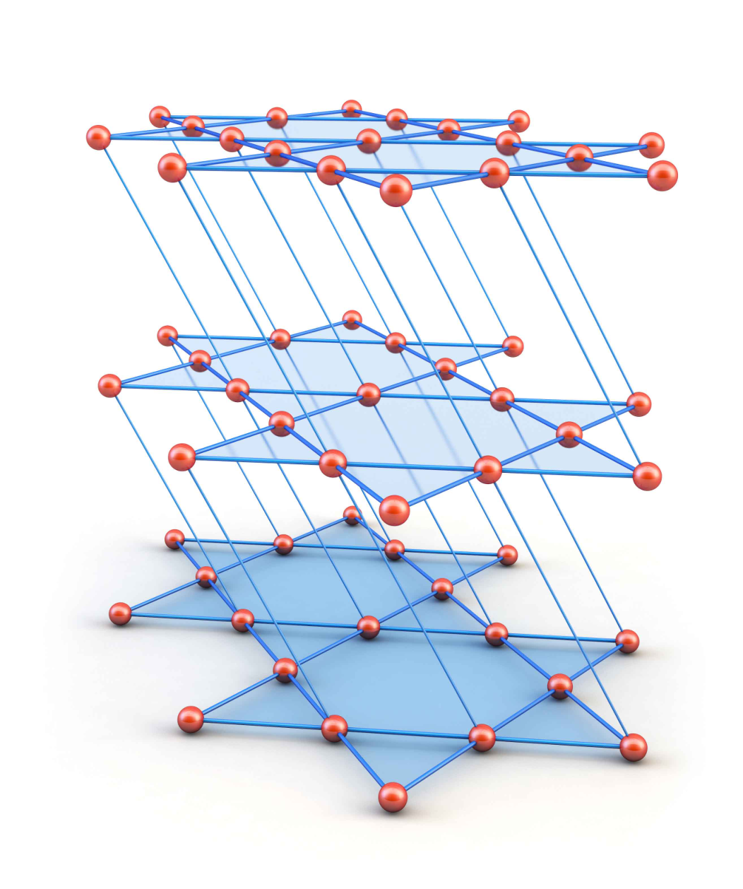
To arrive at a 3D version of the kagome lattice, shown in Fig. 2, we stack the 2D kagome lattices shown in Fig. 1 on top of each other vertically with |a→3|=1|\vec{a}_{3}|=1. Two additional hoppings connect neighboring 2D kagome planes: t1,2​(0,0,1)=2t_{1,2}(0,0,1)=2 and t1,2​(0,1,−1)=2t_{1,2}(0,1,-1)=2. The spectrum is now a function of three reciprocal momenta (k1,k2,k3)(k_{1},k_{2},k_{3}). In Fig. 2-2, we plot three different 3D intersections of the band structure E⁡(k1,k2,k3)E(k_{1},k_{2},k_{3}). All of them contain an anti-𝒫​𝒯\mathcal{PT} flatband at zero energy.

Refer to caption
Refer to caption
Refer to caption
Refer to caption
Refer to caption
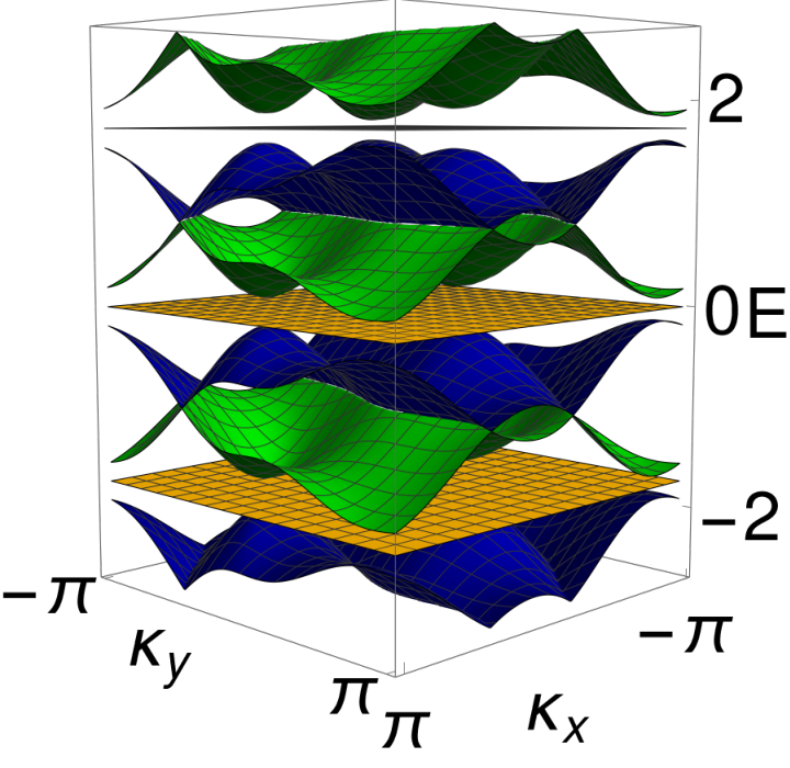
Figure 2: The anti-𝒫​𝒯\mathcal{PT} symmetric generalized 3D kagome lattice. (a)-(c) Three constrained band structures: (a) E⁡(k1,k2,k3=π7)E(k_{1},k_{2},k_{3}=\frac{\pi}{7}), (b) E⁡(k1,k2=π7,k3)E(k_{1},k_{2}=\frac{\pi}{7},k_{3}), (c) E⁡(k1=π7,k2,k3)E(k_{1}=\frac{\pi}{7},k_{2},k_{3}). (d) The lattice structure. The sites are denoted by small solid red spheres. The hopping connections within each 2D kagome plane are the same as in Fig. 1. The intraplane hoppings t1,2​(0,0,1)=2t_{1,2}(0,0,1)=2 and t1,2​(0,1,−1)=2t_{1,2}(0,1,-1)=2. (e) Three subsequent irreducible Wannier-Stark band structures Eγ,a​(κx,κy)E_{\gamma,a}(\kappa_{x},\kappa_{y}) computed using Eq. (16) for the field direction (2,2,3)≡2​a→1+2​a→2+3​a→3(2,2,3)\equiv 2\vec{a}_{1}+2\vec{a}_{2}+3\vec{a}_{3}. The field strength |ℰ→|=7|\vec{\mathcal{E}}|=\sqrt{7}.

Anti-𝒫​𝒯\mathcal{PT} protected Wannier-Stark flatbands.— We now outline and prove the survival of the anti-𝒫​𝒯\mathcal{PT} symmetry in the presence of a uniform DC field ℰ→\vec{\mathcal{E}} for an anti-𝒫​𝒯\mathcal{PT} symmetric Hamiltonian. The DC field adds an on-site potential term in the Hamiltonian (2) and the full Hamiltonian reads

ℋℰ=ℰ→⋅r^+ℋ.\displaystyle\mathcal{H}_{\mathcal{E}}=\vec{\mathcal{E}}\cdot\hat{r}+\mathcal{H}\;. (8)

Here we defined the lattice position operator as r^=∑ν,n→(n→+m→ν)​|ν,n→⟩​⟨ν,n→|\hat{r}=\sum_{\nu,\vec{n}}(\vec{n}+\vec{m}_{\nu})\ket{\nu, \vn}\bra{\nu, \vn}. The DC field term ℰ→⋅r^\vec{\mathcal{E}}\cdot\hat{r} changes sign under the application of the anti-𝒫​𝒯\mathcal{PT} operator 𝒜\mathcal{A} due to lattice reflection 𝒫\mathcal{P}: (n→+m→ν)↦−(n→+m→ν)(\vec{n}+\vec{m}_{\nu})\mapsto-(\vec{n}+\vec{m}_{\nu}). Together with condition (5), this ensures

𝒜⋅ℋℰ⋅𝒜−1=−ℋℰ.\displaystyle\mathcal{A}\cdot\mathcal{H}_{\mathcal{E}}\cdot\mathcal{A}^{-1}=-\mathcal{H}_{\mathcal{E}}. (9)

The application of the uniform DC field breaks translation invariance and eliminates the band structure for generic directions of the DC field. However, for special field directions, translation invariance is broken only partially and a WS band structure emerges as translation invariance is preserved in the direction orthogonal to the field. We refer to such field directions as commensurate Mallick et al. 2021a. The unit cell and sublattice coordinates along the field, zz and zνz_{\nu}, respectively, are defined as z=1ℱ​ℰ→⋅n→,zν=1ℱ​ℰ→⋅m→νz=\frac{1}{\mathcal{F}}\vec{\mathcal{E}}\cdot\vec{n},z_{\nu}=\frac{1}{\mathcal{F}}\vec{\mathcal{E}}\cdot\vec{m}_{\nu} with the scaling factor ℱ\mathcal{F} ensuring that zz taking integer values. The directions perpendicular to ℰ→\vec{\mathcal{E}} are parametrized by a d−1d-1 dimensional integer vector η→\vec{\eta} (see Section .5 of Supplemental Material for details). The Hamiltonian ℋℰ\mathcal{H}_{\mathcal{E}} is translationally invariant in η→\vec{\eta}. With the use of the Bloch basis for η→\vec{\eta},

|ψE​(κ→)⟩=(2​π)1−d2​∑z,ν,η→ψE​(ν,z,κ→)​ei​κ→⋅η→​|ν,z,η→⟩,\displaystyle\ket{\psi_E(\vkp)}={(2\pi)}^{\frac{1-d}{2}}\sum_{z,\nu,\vec{\eta}}\psi_{E}(\nu,z,\vec{\kappa})e^{i\vec{\kappa}\cdot\vec{\eta}}\ket{\nu, z,\vec{\eta}}, (10)

the Hamiltonian (8) becomes block diagonal:

ℋℰ=∫κ→ℋℰ​(κ→)​𝑑κ→,ℋℰ​(κ→)​|ψE​(κ→)⟩=E⁡(κ→)​|ψE​(κ→)⟩.\displaystyle\mathcal{H}_{\mathcal{E}}=\int\limits_{\vec{\kappa}}\mathcal{H}_{\mathcal{E}}(\vec{\kappa})d\vec{\kappa},\quad\mathcal{H}_{\mathcal{E}}(\vec{\kappa})\ket{\psi_E(\vkp)}=E(\vec{\kappa})\ket{\psi_E(\vkp)}. (11)

Each block is infinite dimensional due to the coupling along the zz-direction. The commensurability condition for the DC field implies the persistence of a generalized translational invariance along the field direction, which goes along with an overall shift of the eigenenergies. Following Refs. Kolovsky et al. 2018; Mallick et al. 2021a, we Fourier transform from zz-space to its conjugate momentum qq-space g→E(q,κ→)=(2π)−1/2e−i​E​qℱ∑z,νei​q​(z+zν)ψE(ν,z,κ→)|ν⟩\vec{g}_{E}(q,\vec{\kappa})={(2\pi)}^{-1/2}e^{\frac{-iEq}{\mathcal{F}}}\sum_{z,\nu}e^{iq(z+z_{\nu})}\psi_{E}(\nu,z,\vec{\kappa})\ket{\nu} to arrive at μ\mu coupled differential equations (see Sections .6 and .7 of Supplemental Material for derivation):

i​∂∂q​g→E​(q,κ→)=ℋℰ​(q,κ→)⋅g→E​(q,κ→).\displaystyle i\frac{\partial}{\partial q}\vec{g}_{E}(q,\vec{\kappa})=\mathcal{H}_{\mathcal{E}}(q,\vec{\kappa})\cdot\vec{g}_{E}(q,\vec{\kappa})\;. (12)

The resulting Hermitian Hamiltonian

ℋℰ(q,κ→)=−1ℱ∑l→,ν,σtν,σ(l→)|ν⟩⟨σ|ei​q​(zν−zσ)ei​κ→⋅ϵ→​(l→)−i​q​ℰ→⋅l→ℱ\displaystyle\mathcal{H}_{\mathcal{E}}(q,\vec{\kappa})=-\frac{1}{\mathcal{F}}\sum_{\vec{l},\nu,\sigma}t_{\nu,\sigma}(\vec{l})\outerproduct{\nu}{\sigma}e^{iq(z_{\nu}-z_{\sigma})}e^{i\vec{\kappa}\cdot\vec{\epsilon}(\vec{l})-\frac{iq\vec{\mathcal{E}}\cdot\vec{l}}{\mathcal{F}}} (13)

is a μ×μ\mu\times\mu matrix which acts on the sublattice space {|ν⟩}\{\ket{\nu}\} only, ϵ→​(l→)\vec{\epsilon}(\vec{l}) is the hopping perpendicular to the field. Equation (12) describes a unitary evolution of g→E​(q,κ→)\vec{g}_{E}(q,\vec{\kappa}) in qq-space,

g→E​(q,κ→)=U⁡(q,κ→)⋅g→E​(0,κ→),\displaystyle\vec{g}_{E}(q,\vec{\kappa})=U(q,\vec{\kappa})\cdot\vec{g}_{E}(0,\vec{\kappa}), (14)

where U⁡(q,κ→)U(q,\vec{\kappa}) is a qq-ordered exponential of the integrated ℋℰ​(q,κ→)\mathcal{H}_{\mathcal{E}}(q,\vec{\kappa}):

U⁡(q,κ→)=𝟙+(−i)​∫q′=0qd​q′​ℋℰ​(q′,κ→)\displaystyle U(q,\vec{\kappa})=\mathds{1}+(-i)\int_{q^{\prime}=0}^{q}dq^{\prime}\mathcal{H}_{\mathcal{E}}(q^{\prime},\vec{\kappa})
+(−i)2∫q′=0q∫q′′=0q′dq′dq′′ℋℰ(q′,κ→)ℋℰ(q′′,κ→)+⋯.\displaystyle+{(-i)}^{2}\int_{q^{\prime}=0}^{q}\int_{q^{\prime\prime}=0}^{q^{\prime}}dq^{\prime}dq^{\prime\prime}\mathcal{H}_{\mathcal{E}}(q^{\prime},\vec{\kappa})\mathcal{H}_{\mathcal{E}}(q^{\prime\prime},\vec{\kappa})+\cdots\;. (15)

By construction, g→E​(2​π,κ→)=e−2​π​i​Eℱ​Λ​(2​π)⋅g→E​(0,κ→)\vec{g}_{E}(2\pi,\vec{\kappa})=e^{-\frac{2\pi iE}{\mathcal{F}}}\Lambda(2\pi)\cdot\vec{g}_{E}(0,\vec{\kappa}), where the matrix Λ⁡(q)\Lambda(q) is diagonal with entries Λν​ν​(q)=ei​q​zν\Lambda_{\nu\nu}(q)=e^{iqz_{\nu}}. Then, from Eq. (14) and the above periodicity condition, we arrive at the eigenvalue problem on the WS bands:

[Λ†​(2​π)⋅U⁡(2​π,κ→)]⋅g→E​(0,κ→)=e−2​π​i​Eℱ​g→E​(0,κ→).\displaystyle\big[\Lambda^{\dagger}(2\pi)\cdot U(2\pi,\vec{\kappa})\big]\cdot\vec{g}_{E}(0,\vec{\kappa})=e^{-\frac{2\pi iE}{\mathcal{F}}}\vec{g}_{E}(0,\vec{\kappa})\;. (16)

The spectrum of ℋℰ\mathcal{H}_{\mathcal{E}} is obtained by solving the above eigenproblem,

E≡Eγ,a​(κ→)=ℱ​a+i​ℱ2​π​ln⁡[λγ​(κ→)],\displaystyle E\equiv E_{\gamma,a}(\vec{\kappa})=\mathcal{F}a+\frac{i\mathcal{F}}{2\pi}\ln\left[\lambda_{\gamma}(\vec{\kappa})\right], (17)

where a∈ℤa\in\mathbb{Z} and λγ\lambda_{\gamma} are the eigenvalues of the μ×μ\mu\times\mu unitary matrix Λ†​(2​π)⋅U⁡(2​π,κ→)\Lambda^{\dagger}(2\pi)\cdot U(2\pi,\vec{\kappa}). The irreducible WS band structure is obtained by choosing a particular value of aa, e.g., a=0a=0. The entire spectrum is generated by a parallel shift of the irreducible band structure and is parametrized by the band indices (γ,a)(\gamma,a).

We now arrive at the formulation of our anti-𝒫​𝒯\mathcal{PT} theorem in the presence of the commensurate DC field: If the original Hamiltonian ℋ\mathcal{H} has an odd number of sublattices and is anti-𝒫​𝒯\mathcal{PT} symmetric, the irreducible WS band structure of ℋℰ\mathcal{H}_{\mathcal{E}} contains at least one flatband.

Proof: Indeed, the anti-𝒫​𝒯\mathcal{PT} condition (9) translates into a similar condition for the effective Hamiltonian ℋℰ​(q,κ→)\mathcal{H}_{\mathcal{E}}(q,\vec{\kappa}),

ℋℰ∗(q,κ→)=−ℳ†(κ→)⋅ℋℰ(q,κ→)⋅ℳ(κ→),\displaystyle\mathcal{H}_{\mathcal{E}}^{*}(q,\vec{\kappa})=-\mathcal{M}^{\dagger}(\vec{\kappa})\cdot\mathcal{H}_{\mathcal{E}}(q,\vec{\kappa})\cdot\mathcal{M}(\vec{\kappa}), (18)

where the μ×μ\mu\times\mu unitary matrix

ℳ⁡(κ→)=∑νe−i​ξν​ei​κ→⋅ϵ→​(p→ν)​|f⁡(ν)⟩⟨ν|.\displaystyle\mathcal{M}(\vec{\kappa})=\sum_{\nu}e^{-i\xi_{\nu}}e^{i\vec{\kappa}\cdot\vec{\epsilon}(\vec{p}_{\nu})}\outerproduct{f(\nu)}{\nu}. (19)

ϵ→​(p→ν)\vec{\epsilon}(\vec{p}_{\nu}) is the same vector function of l→\vec{l} as in Eq. (13) but its argument is replaced by p→ν\vec{p}_{\nu}. Then, from Eq. (15) it is straightforward to establish that

U∗​(q,κ→)=ℳ†​(κ→)⋅U⁡(q,κ→)⋅ℳ⁡(κ→).\displaystyle U^{*}(q,\vec{\kappa})=\mathcal{M}^{\dagger}(\vec{\kappa})\cdot U(q,\vec{\kappa})\cdot\mathcal{M}(\vec{\kappa}). (20)

We note that by definition of the commensurate DC field direction, the projection of p→ν\vec{p}_{\nu} along the field direction will be an integer and hence (zν+zf⁡(ν))(z_{\nu}+z_{f(\nu)}) will be an integer as well (see Section .8 of Supplemental Material for details). Therefore, e2​π​i​(zν+zf⁡(ν))=1e^{2\pi i(z_{\nu}+z_{f(\nu)})}=1. Since the operator ℳ⁡(κ→)\mathcal{M}(\vec{\kappa}) maps the sublattice vector |ν⟩\ket{\nu} to |f⁡(ν)⟩\ket{f(\nu)}, it follows that

Λ†​(2​π)=ℳ⁡(κ→)⋅Λ⁡(2​π)⋅ℳ†​(κ→).\displaystyle\Lambda^{\dagger}(2\pi)=\mathcal{M}(\vec{\kappa})\cdot\Lambda(2\pi)\cdot\mathcal{M}^{\dagger}(\vec{\kappa})\;. (21)

We use the relations (20) and (21) to rewrite the eigenvalue problem (16) into the following form (see Section .8 of Supplemental Material):

[Λ†​(2​π)⋅U⁡(2​π,κ→)]⋅[ℳ⁡(κ→)⋅g→E∗​(0,κ→)]\displaystyle\left[\Lambda^{\dagger}(2\pi)\cdot U(2\pi,\vec{\kappa})\right]\cdot\big[\mathcal{M}(\vec{\kappa})\cdot\vec{g}^{*}_{E}(0,\vec{\kappa})\big]
=e2​π​i​Eℱ​[ℳ⁡(κ→)⋅g→E∗​(0,κ→)].\displaystyle=e^{\frac{2\pi iE}{\mathcal{F}}}\big[\mathcal{M}(\vec{\kappa})\cdot\vec{g}^{*}_{E}(0,\vec{\kappa})\big]\;. (22)

Equations (16) and (22) imply that the eigenvalues of the unitary operator [Λ†​(2​π)⋅U⁡(2​π,κ→)][\Lambda^{\dagger}(2\pi)\cdot U(2\pi,\vec{\kappa})] come in pairs (e−2​π​i​E​(κ→)ℱ,e2​π​i​E​(κ→)ℱ)(e^{-\frac{2\pi iE(\vec{\kappa})}{\mathcal{F}}},e^{\frac{2\pi iE(\vec{\kappa})}{\mathcal{F}}}). For an odd number of sublattices μ\mu, the number of eigenvalues of the operator [Λ†​(2​π)⋅U⁡(2​π,κ→)][\Lambda^{\dagger}(2\pi)\cdot U(2\pi,\vec{\kappa})] is also odd. Therefore, at least one eigenvalue satisfies e−2​π​i​E​(κ→)ℱ=e2​π​i​E​(κ→)ℱe^{-\frac{2\pi iE(\vec{\kappa})}{\mathcal{F}}}=e^{\frac{2\pi iE(\vec{\kappa})}{\mathcal{F}}} with E⁡(κ→)E(\vec{\kappa}) being κ→\vec{\kappa} independent and a multiple of ℱ2\frac{\mathcal{F}}{2}. Therefore, the irreducible WS band structure contains at least one anti-𝒫​𝒯\mathcal{PT} symmetry protected flatband. □\square

We check the validity of the above theorem by computing WS band structures with (16) for the 2D kagome lattice in Fig. 1 and 3D kagome lattice in Fig. 2. Details on the field direction and strength are provided in the corresponding captions. We observe and confirm the presence of anti-𝒫​𝒯\mathcal{PT} protected WS flatbands in Fig. 1 for the 2D case and in Fig. 2 for the 3D case.

Experimental realizations.— Flatband models have already been designed in metallic systems Kajiwara et al. 2016, photonic lattices Zong et al. 2016; Mukherjee and Thomson 2017; Xia et al. 2016; Xia et al. 2020; Yan et al. 2020; Tang et al. 2020, and ultracold atoms in optical lattices Jo et al. 2012. The unperturbed kagome lattices introduced above can be tested in similar setups Zong et al. 2016; Jo et al. 2012 by proper design of hopping parameters with artificial gauge fields.

To observe the Wannier-Stark effect in optical lattices with ultracold atomic gases, they can be tilted, so the gravitational field acts as a DC field source Anderson and Kasevich 1998. Moreover, one can study the impact of an electric DC field on centrosymmetric lattices as reported in a very recent experiment on diamond De Santis et al. 2021. Another option for implementing the WS Hamiltonians is to use Floquet engineering following recent experiments, which implemented Floquet Hamiltonians using ultracold atoms Bordia et al. 2017; Eckardt 2017. The spectrum of WS Hamiltonians can be mapped onto that of periodically driven systems Oka and Kitamura 2019 and vise versa. Mapping the frequency-space of a Floquet (d−1)(d-1)-dimensional lattice Hamiltonian to a new spatial dimension produces an effective static Hamiltonian in a dd-dimensional lattice with WS potential. In this case, the single set of Floquet bands, which are periodic in energy, unfolds into an infinitely repeated tower of Wannier-Stark bands. The details of the mapping between our WS Hamiltonians in 2D (3D) kagome networks and the Hamiltonians having Floquet Peierls phases in 1D (2D) diamond lattices are provided in Section .9 of the Supplemental Material.

Discussion and conclusions.— We considered tight-binding lattice Hamiltonians on dd-dimensional non-Bravais lattices, which are invariant under the anti-𝒫​𝒯\mathcal{PT} symmetry. We proved that the anti-𝒫​𝒯\mathcal{PT} symmetry protects a flatband at energy E=0E=0 for odd numbers of sublattices. We derived the precise anti-𝒫​𝒯\mathcal{PT} constraints on the Hamiltonian and used them to generate examples of generalized kagome networks. Remarkably the anti-𝒫​𝒯\mathcal{PT} symmetry persists in the presence of uniform DC fields. We prove that the corresponding irreducible Wannier-Stark band structures will again contain anti-𝒫​𝒯\mathcal{PT} protected flatbands. We demonstrate the validity of our results by computing examples of the Wannier-Stark band structure of generalized 2D and 3D kagome networks in the presence of DC fields.

The zero-energy flatbands reported in Refs. Green et al. 2010; Koch et al. 2010; Wei and Sedrakyan 2021; Chen et al. 2014 belong to the anti-𝒫​𝒯\mathcal{PT} class. They were reported for specific choices of hoppings for two-dimensional lattices. Our results also explain the persistence of the flatband in the dice lattice Kolovsky et al. 2018 in the presence of the DC field. The original proof relied on specific properties of the hopping network, and subsequent conjectures attempted to connect the proof to the bipartiteness of the unbiased lattice. Actually, the unbiased dice lattice is both chiral and anti-𝒫​𝒯\mathcal{PT} symmetric. Therefore, its E=0E=0 flatband is protected by both the chiral and the anti-𝒫​𝒯\mathcal{PT} symmetries. Adding a DC field destroys the chiral symmetry but preserves the anti-𝒫​𝒯\mathcal{PT} symmetry. Therefore, the emerging WS flatbands in the irreducible WS band structure are protected by the anti-𝒫​𝒯\mathcal{PT} symmetry. Anti-𝒫​𝒯\mathcal{PT} networks do not need to be bipartite and our proof is valid for any dd-dimension with arbitrary number of sublattices.

Our study focused on spinless single particle translationally invariant Hermitian Hamiltonians on non-Bravais lattices. Our results also apply to a particle with an integer spin (or other internal degrees of freedom, e.g., orbital degrees of freedom) including spin-orbit coupling on a Bravais lattice. The impact of disorder, many-body interactions, nonlinearities, or non-Hermiticity on our system are possible interesting directions for future investigations. We expect that methods developed to analyze the impact of these perturbations for other flatband models might be helpful in our setting as well. It is also interesting to study the case of incommensurate DC field directions that are expected to generate quasicrystalline structures.

Acknowledgments.— This work was supported by Institute for Basic Science in Korea (No. IBS-R024-D1). N.C. acknowledges financial support from the China Scholarship Council (No. CSC-201906040021). We thank Jung-Wan Ryu for helpful discussions.

Supplemental Material: Anti-𝒫​𝒯\mathcal{PT} flatbands

.1 Anti-𝒫​𝒯\mathcal{PT} symmetry conditions for (sub)lattice vectors

We label every lattice site r→\vec{r} by its unit cell index vector n→=∑i=1dni​a→i\vec{n}=\sum_{i=1}^{d}n_{i}\vec{a}_{i} and a sublattice index ν=1,2,…​μ\nu=1,2,\ldots\mu where μ\mu is the number of sublattices. Here a→i\vec{a}_{i} is the lattice basis vector for unit cell, μ\mu is the number of sublattices, and nin_{i} always take integer values. Note that the vectors a→1,a→2,…,a→d\vec{a}_{1},\vec{a}_{2},\dots,\vec{a}_{d} are complete and linearly independent, but they need not to be orthogonal nor normal. We can express sublattice positions measured with respect to a unit cell vector n→\vec{n}, in terms of the basis vectors: m→ν=∑i=1dmν,i​a→i\vec{m}_{\nu}=\sum_{i=1}^{d}m_{\nu,i}\vec{a}_{i} with |mν,i|<1|m_{\nu,i}|<1 for all ν,i\nu,i. The combination ν,n→\nu,\vec{n} uniquely identifies the lattice vector r→=m→ν+n→≡(ν,n→)\vec{r}=\vec{m}_{\nu}+\vec{n}\equiv(\nu,\vec{n}). Therefore we can use them to label the Hilbert space basis vectors as |ν,n→⟩\ket{\nu, \vn}. The lattice shift vector p→ν\vec{p}_{\nu} can also be written as: p→ν=∑i=1dpν,i​a→i\vec{p}_{\nu}=\sum_{i=1}^{d}p_{\nu,i}\vec{a}_{i} where pν,ip_{\nu,i} are integers.

The reflection of the position operator

r^=∑n→,ν(m→ν+n→)​|ν,n→⟩⟨ν,n→|\displaystyle\hat{r}=\sum_{\vec{n},\nu}(\vec{m}_{\nu}+\vec{n})\outerproduct{\nu, \vn}{\nu, \vn}

under the antisymmetry operation 𝒜\mathcal{A} reads

𝒜⋅r^⋅𝒜−1=−r^;\displaystyle\mathcal{A}\cdot\hat{r}\cdot\mathcal{A}^{-1}=-\hat{r}~;
⇒∑n→,ν(m→ν+n→)|f⁡(ν),−n→−p→ν⟩⟨f⁡(ν),−n→−p→ν|=−∑n→,ν(m→f⁡(ν)+n→)|f⁡(ν),n→⟩⟨f⁡(ν),n→|\displaystyle\Rightarrow\sum_{\vec{n},\nu}(\vec{m}_{\nu}+\vec{n})\outerproduct{f(\nu), -\vn- \vec{p}_\nu}{f(\nu), -\vn- \vec{p}_\nu}=-\sum_{\vec{n},\nu}(\vec{m}_{f(\nu)}+\vec{n})\outerproduct{f(\nu), \vn}{f(\nu), \vn}
⇒∑n→,ν(m→ν−n→−p→ν)|f⁡(ν),n→⟩⟨f⁡(ν),n→|=−∑n→,ν(m→f⁡(ν)+n→)|f⁡(ν),n→⟩⟨f⁡(ν),n→|⇒m→ν−p→ν=−m→f⁡(ν).\displaystyle\Rightarrow\sum_{\vec{n},\nu}(\vec{m}_{\nu}-\vec{n}-\vec{p}_{\nu})\outerproduct{f(\nu), \vn}{f(\nu),\vn}=-\sum_{\vec{n},\nu}(\vec{m}_{f(\nu)}+\vec{n})\outerproduct{f(\nu), \vn}{f(\nu), \vn}\Rightarrow\vec{m}_{\nu}-\vec{p}_{\nu}=-\vec{m}_{f(\nu)}\;. (23)

By definition the sublattice vectors satisfy 0≤|mν,i|<1,0≤|mf⁡(ν),i|<10\leq|m_{\nu,i}|<1,0\leq|m_{f(\nu),i}|<1 and pi​(ν)p_{i}(\nu) is always integer. Therefore the components of the shift vector p→ν\vec{p}_{\nu} can only take values from {0,±1}\{0,\pm 1\} for any ν\nu.

.2 Implications of 𝒜2∝𝟙\mathcal{A}^{2}\propto\mathds{1}

The operator 𝒜\mathcal{A} consists of a spatial reflection and a complex conjugation operation in position basis:

𝒜=𝒯⋅𝒫=𝒯⋅∑ν,n→ei​ξν​|f⁡(ν),−n→−p→ν⟩⟨ν,n→|.\displaystyle\mathcal{A}=\mathcal{T}\cdot\mathcal{P}=\mathcal{T}\cdot\sum_{\nu,\vec{n}}e^{i\xi_{\nu}}\outerproduct{f(\nu), -\vn- \vec{p}_\nu}{\nu, \vn}. (24)

Therefore, when 𝒜\mathcal{A} acts on an arbitrary state two times, it should return the same state up to an overall phase factor ei​Ωe^{i\Omega} :

𝒜2\displaystyle\mathcal{A}^{2} =𝒯⋅∑ν,n→ei​ξν​|f⁡(ν),−n→−p→ν⟩⟨ν,n→|⋅𝒯⋅∑σ,n→′ei​ξσ​|f⁡(σ),−n→′−p→σ⟩⟨σ,n→′|\displaystyle=\mathcal{T}\cdot\sum_{\nu,\vec{n}}e^{i\xi_{\nu}}\outerproduct{f(\nu), -\vn- \vec{p}_\nu}{\nu, \vn}\cdot\mathcal{T}\cdot\sum_{\sigma,\vec{n}^{\prime}}e^{i\xi_{\sigma}}\outerproduct{f(\sigma), -\vn' - \vec{p}_\sigma}{\sigma, \vn'}
=∑ν,n→,σ,n→′e−i​ξν+i​ξσ​|f⁡(ν),−n→−p→ν⟩⟨σ,n→′|​δν,f⁡(σ)​δn→,−n→′−p→σ\displaystyle=\sum_{\nu,\vec{n},\sigma,\vec{n}^{\prime}}e^{-i\xi_{\nu}+i\xi_{\sigma}}\outerproduct{f(\nu), -\vn- \vec{p}_\nu}{\sigma, \vn'}\delta_{\nu,f(\sigma)}\delta_{\vec{n},-\vec{n}^{\prime}-\vec{p}_{\sigma}}
=∑σ,n→′e−i​ξf⁡(σ)+i​ξσ​|σ,n→′+p→σ−p→f⁡(σ)⟩⟨σ,n→′|=ei​Ω​𝟙\displaystyle=\sum_{\sigma,\vec{n}^{\prime}}e^{-i\xi_{f(\sigma)}+i\xi_{\sigma}}\outerproduct{\sigma, \vn' + \vec{p}_\sigma- \vec{p}_{f(\sigma)}}{\sigma, \vn'}=e^{i\Omega}\mathds{1} (25)

where we used the fact that ff is its own inverse: f⁡(f⁡(σ))=σf(f(\sigma))=\sigma. 𝟙\mathds{1} is the identity operator both in the sublattice space as well as in the unit cell position space. Therefore for all σ\sigma

ξσ−ξf⁡(σ)=Ωmod2​π,\displaystyle\xi_{\sigma}-\xi_{f(\sigma)}=\Omega\mod 2\pi,
p→σ=p→f⁡(σ).\displaystyle\vec{p}_{\sigma}=\vec{p}_{f(\sigma)}. (26)

The condition 𝒜2≡𝟙\mathcal{A}^{2}\equiv\mathds{1} is equivalent to the particle-hole symmetry requirement (see Ref. Chiu et al. 2016 for details). The Hamiltonian can be classified topologically according to the value of Ω\Omega, the presence of time-reversal and chiral symmetries. If f⁡(σ)=σf(\sigma)=\sigma for at least one sublattice σ\sigma the condition Eq. (26) implies Ω=0\Omega=0 and therefore 𝒜2=𝟙\mathcal{A}^{2}=\mathds{1}. This happens for example, for an odd number of sublattices.

.3 Conditions on the hopping matrices under anti-𝒫​𝒯\mathcal{PT} symmetry of the Hamiltonian

The Hamiltonian is given by

ℋ=−∑l→,n→∑ν,σ=1μtν,σ(l→)|ν,n→⟩⟨σ,n→+l→|such thattν,σ∗(l→)=tσ,ν(−l→).\displaystyle\mathcal{H}=-\sum_{\vec{l},\vec{n}}\sum_{\nu,\sigma=1}^{\mu}t_{\nu,\sigma}(\vec{l})\outerproduct{\nu, \vn}{\sigma, \vn+ \vec{l}}\quad\text{such that}~t^{*}_{\nu,\sigma}(\vec{l})=t_{\sigma,\nu}(-\vec{l}). (27)

Under the action of 𝒜\mathcal{A} (24) we demand

𝒜⋅ℋ⋅𝒜−1=−ℋ\displaystyle\mathcal{A}\cdot\mathcal{H}\cdot\mathcal{A}^{-1}=-\mathcal{H}
⇒∑l→,n→∑ν,σ=1μe−i​ξν+i​ξσtν,σ∗(l→)|f⁡(ν),−n→−p→ν⟩⟨f⁡(σ),−n→−l→−p→σ|=−∑l→,n→∑ν,σ=1μtf⁡(ν),f⁡(σ)(l→)|f⁡(ν),n→⟩⟨f⁡(σ),n→+l→|\displaystyle\Rightarrow\sum_{\vec{l},\vec{n}}\sum_{\nu,\sigma=1}^{\mu}e^{-i\xi_{\nu}+i\xi_{\sigma}}t^{*}_{\nu,\sigma}(\vec{l})\outerproduct{f(\nu), -\vn- \vec{p}_\nu}{f(\sigma), -\vn- \vec{l} - \vec{p}_\sigma}=-\sum_{\vec{l},\vec{n}}\sum_{\nu,\sigma=1}^{\mu}t_{f(\nu),f(\sigma)}(\vec{l})\outerproduct{f(\nu), \vn}{f(\sigma), \vn+ \vec{l}}
⇒∑l→,n→∑ν,σ=1μe−i​ξν+i​ξσtν,σ∗(l→)|f⁡(ν),n→⟩⟨f⁡(σ),n→−l→+p→ν−p→σ|=−∑l→,n→∑ν,σ=1μtf⁡(ν),f⁡(σ)(l→)|f⁡(ν),n→⟩⟨f⁡(σ),n→+l→|\displaystyle\Rightarrow\sum_{\vec{l},\vec{n}}\sum_{\nu,\sigma=1}^{\mu}e^{-i\xi_{\nu}+i\xi_{\sigma}}t^{*}_{\nu,\sigma}(\vec{l})\outerproduct{f(\nu), \vn}{f(\sigma), \vn- \vec{l} + \vec{p}_\nu- \vec{p}_\sigma}=-\sum_{\vec{l},\vec{n}}\sum_{\nu,\sigma=1}^{\mu}t_{f(\nu),f(\sigma)}(\vec{l})\outerproduct{f(\nu), \vn}{f(\sigma), \vn+ \vec{l}}
⇒e−i​ξν+i​ξσ​tν,σ∗​(l→)=−tf⁡(ν),f⁡(σ)​(−l→+p→ν−p→σ).\displaystyle\Rightarrow e^{-i\xi_{\nu}+i\xi_{\sigma}}t^{*}_{\nu,\sigma}(\vec{l})=-t_{f(\nu),f(\sigma)}(-\vec{l}+\vec{p}_{\nu}-\vec{p}_{\sigma})~. (28)

Note that the derivation of the condition (28) did not impose any constraint on p→ν\vec{p}_{\nu}: its components pν,ip_{\nu,i} can take any integer values. Enforcing the anti-𝒫​𝒯\mathcal{PT} symmetry on a lattice, restricts the possible values of the components of p→ν\vec{p}_{\nu} as was described in Section .1. However the above result suggests possible generalizations for Hamiltonians on generic graphs, provided a suitable generalization for the reflection operator is given.

.4 Anti-𝒫​𝒯\mathcal{PT} symmetric generalized kagome lattice

We choose the following unit cell basis vectors for the 3D kagome lattice:

a→1=e^1,a→2=12​e^1+32​e^2,a→3=e^3.\displaystyle\vec{a}_{1}=\hat{e}_{1},\vec{a}_{2}=\frac{1}{2}\hat{e}_{1}+\frac{\sqrt{3}}{2}\hat{e}_{2},~\vec{a}_{3}=\hat{e}_{3}\;. (29)

where e^1,e^2,e^3\hat{e}_{1},\hat{e}_{2},\hat{e}_{3} are the Cartesian orthonormal coordinate axes. Therefore we have n→=n1​a→1+n2​a→2+n3​a→3\vec{n}=n_{1}\vec{a}_{1}+n_{2}\vec{a}_{2}+n_{3}\vec{a}_{3}, l→=l1​a→1+l2​a→2+l3​a→3\vec{l}=l_{1}\vec{a}_{1}+l_{2}\vec{a}_{2}+l_{3}\vec{a}_{3}, p→1=a→2\vec{p}_{1}=\vec{a}_{2}, p→2=0→\vec{p}_{2}=\vec{0}, p→3=a→1\vec{p}_{3}=\vec{a}_{1}, f⁡(ν)=νf(\nu)=\nu.

The anti-𝒫​𝒯\mathcal{PT} symmetry constrains the hopping parameters as implied by Eq. (28)

|t1,2​(0,0,0)|=|t1,2​(0,1,0)|,|t1,3​(0,0,0)|=|t3,1​(1,−1,0)|,\displaystyle|t_{1,2}(0,0,0)|=|t_{1,2}(0,1,0)|,|t_{1,3}(0,0,0)|=|t_{3,1}(1,-1,0)|,
|t2,3​(0,0,0)|=|t2,3​(−1,0,0)|,|t1,2​(0,0,1)|=|t1,2​(0,1,−1)|.\displaystyle|t_{2,3}(0,0,0)|=|t_{2,3}(-1,0,0)|,|t_{1,2}(0,0,1)|=|t_{1,2}(0,1,-1)|.
arg⁡(t1,2​(0,1,0))=π−arg⁡(t1,2​(0,0,0))−ξ1+ξ2​mod​2​π,\displaystyle\arg(t_{1,2}(0,1,0))=\pi-\arg(t_{1,2}(0,0,0))-\xi_{1}+\xi_{2}~\text{mod}~2\pi,
arg⁡(t3,1​(1,−1,0))=π+arg⁡(t1,3​(0,0,0))+ξ1−ξ3​mod​2​π,\displaystyle\arg(t_{3,1}(1,-1,0))=\pi+\arg(t_{1,3}(0,0,0))+\xi_{1}-\xi_{3}~\text{mod}~2\pi,
arg⁡(t2,3​(−1,0,0))=π−arg⁡(t2,3​(0,0,0))−ξ2+ξ3​mod​2​π,\displaystyle\arg(t_{2,3}(-1,0,0))=\pi-\arg(t_{2,3}(0,0,0))-\xi_{2}+\xi_{3}~\text{mod}~2\pi,
arg⁡(t1,2​(0,1,−1))=π−arg⁡(t1,2​(0,0,1))−ξ1+ξ2​mod​2​π,\displaystyle\arg(t_{1,2}(0,1,-1))=\pi-\arg(t_{1,2}(0,0,1))-\xi_{1}+\xi_{2}~\text{mod}~2\pi, (30)

and all the other hoppings equal zero. We consider a special class of examples which satisfy the conditions (.4) in the main text:

|t1,2​(0,0,0)|=|t1,2​(0,1,0)|=t=0.15,\displaystyle|t_{1,2}(0,0,0)|=|t_{1,2}(0,1,0)|=t=0.15,
|t1,3​(0,0,0)|=|t3,1​(1,−1,0)|=|t2,3​(0,0,0)|=|t2,3​(−1,0,0)|=1,\displaystyle|t_{1,3}(0,0,0)|=|t_{3,1}(1,-1,0)|=|t_{2,3}(0,0,0)|=|t_{2,3}(-1,0,0)|=1,
|t1,2​(0,0,1)|=|t1,2​(0,1,−1)|=s.\displaystyle|t_{1,2}(0,0,1)|=|t_{1,2}(0,1,-1)|=s.
arg⁡(t3,1​(1,−1,0))=π,arg⁡(t2,3​(0,0,0))=−arg⁡(t2,3​(−1,0,0))=φ=π5,\displaystyle\arg(t_{3,1}(1,-1,0))=\pi,\arg(t_{2,3}(0,0,0))=-\arg(t_{2,3}(-1,0,0))=\varphi=\frac{\pi}{5},
arg⁡(t1,2​(0,1,0))=arg⁡(t1,3​(0,0,0))=arg⁡(t1,2​(0,0,0))=arg⁡(t1,2​(0,0,1))=arg⁡(t1,2​(0,1,−1))=0.\displaystyle\arg(t_{1,2}(0,1,0))=\arg(t_{1,3}(0,0,0))=\arg(t_{1,2}(0,0,0))=\arg(t_{1,2}(0,0,1))=\arg(t_{1,2}(0,1,-1))=0~. (31)

Diagonalizing the Hamiltonian ℋ⁡(k→)\mathcal{H}(\vec{k}) with these choices of parameters (t,φ,s)(t,\varphi,s) we obtain three bands:

E=0,±[2s2cos⁡(k2−2​k3)+4tscos⁡(k2−k3)+4tscos⁡(k3)+2t2cos⁡(k2)\displaystyle E=0,\pm\big[2s^{2}\cos(k_2-2 k_3)+4ts\cos(k_2-k_3)+4ts\cos(k_3)+2t^{2}\cos(k_2)
+2cos⁡(k1+2​φ)−2cos⁡(k1−k2)+2s2+2t2+4]12.\displaystyle+2\cos(k_1+2 \varphi)-2\cos(k_1-k_2)+2s^{2}+2t^{2}+4\big]^{\frac{1}{2}}. (32)

Therefore this choice of hoppings supports a flatband at E=0E=0. For the two dimensional kagome case we set s=0s=0 and for the three dimensional case we set s=2s=2. The corresponding flatband eigenstate forms a compact localized state occupying five (three) unit cells in 3D (2D):

14+2​t2+2​s2[\displaystyle\frac{1}{\sqrt{4+2t^{2}+2s^{2}}}\Big[ |ν=1⟩⊗{e−i​φ​|n1+1,n2,n3⟩+ei​φ​|n1,n2,n3⟩}\displaystyle\ket{\nu= 1}\otimes\big\{e^{-i\varphi}\ket{n_1 + 1, n_2, n_3}+e^{i\varphi}\ket{n_1, n_2, n_3}\big\}
+\displaystyle+ |ν=2⟩⊗{|n1,n2+1,n3⟩−|n1+1,n2,n3⟩}\displaystyle\ket{\nu= 2}\otimes\big\{\ket{n_1, n_2 + 1, n_3}-\ket{n_1 + 1, n_2, n_3}\big\}
−\displaystyle- |ν=3⟩⊗{t|n1,n2+1,n3⟩+t|n1,n2,n3⟩+s|n1,n2,n3+1⟩+s|n1,n2+1,n3−1⟩}].\displaystyle\ket{\nu= 3}\otimes\big\{t\ket{n_1, n_2 + 1, n_3}+t\ket{n_1, n_2, n_3}+s\ket{n_1, n_2, n_3 + 1}+s\ket{n_1, n_2 + 1, n_3 - 1}\big\}\Big]~. (33)

.5 Parametrization of DC field coordinates

In this section we define the coordinates along and perpendicular to the DC field and present a way to parametrize these new coordinates. We express the uniform DC field in a dd-dimensional lattice in terms of the unit-cell basis vectors a→j\vec{a}_{j}:

ℰ→=∑j=1dℰj​a→j.\displaystyle\vec{\mathcal{E}}=\sum_{j=1}^{d}\mathcal{E}_{j}\vec{a}_{j}. (34)

We define the coordinate along the DC field as

z=1ℱ​ℰ→⋅n→=1ℱ​∑j=1dℰj​a→j⋅∑i=1dni​a→i=∑i=1dni​ℰℱ​i,ℰℱ​i=1ℱ​∑j=1dℰj​(a→j⋅a→i),\displaystyle z=\frac{1}{\mathcal{F}}\vec{\mathcal{E}}\cdot\vec{n}=\frac{1}{\mathcal{F}}\sum_{j=1}^{d}\mathcal{E}_{j}\vec{a}_{j}\cdot\sum_{i=1}^{d}n_{i}\vec{a}_{i}=\sum_{i=1}^{d}n_{i}\mathcal{E}_{\mathcal{F}i},\qquad\mathcal{E}_{\mathcal{F}i}=\frac{1}{\mathcal{F}}\sum_{j=1}^{d}\mathcal{E}_{j}\left(\vec{a}_{j}\cdot\vec{a}_{i}\right), (35)

where ℱ\mathcal{F} is a proportionality factor to be specified later. Similar to the unit cell coordinate along the field zz we define the sublattice coordinate along the field:

zν=∑j=1dmν,j​ℰℱ​j.\displaystyle z_{\nu}=\sum_{j=1}^{d}m_{\nu,j}\mathcal{E}_{\mathcal{F}j}\;. (36)

If the field direction is commensurate Mallick et al. 2021a we can find (d−1)(d-1) vectors {ℰ→⟂(s):s=2,3,…,d}\{\vec{\mathcal{E}}^{\perp}(s):s=2,3,\ldots,d\} perpendicular to the field, and all of them can be expressed through unit-cell lattice vectors ℰ→⟂​(s)=∑iℰi⟂​(s)​a→i\vec{\mathcal{E}}^{\perp}(s)=\sum_{i}\mathcal{E}^{\perp}_{i}(s)\vec{a}_{i} where ℰi⟂​(s)∈ℤ\mathcal{E}^{\perp}_{i}(s)\in\mathbb{Z}. The corresponding orthogonality condition reads

ℰ→⋅ℰ→⟂​(s)=0⇒∑i=1dℰi⟂​(s)​ℰℱ​i=0∀s.\displaystyle\vec{\mathcal{E}}\cdot\vec{\mathcal{E}}^{\perp}(s)=0\Rightarrow\sum_{i=1}^{d}\mathcal{E}^{\perp}_{i}(s)\mathcal{E}_{\mathcal{F}i}=0\qquad\forall s. (37)

Equation (37) is a set of d−1d-1 degenerate linear equations for dd real variables ℰℱ​i\mathcal{E}_{\mathcal{F}i} with integer coefficients ℰi⟂​(s)\mathcal{E}^{\perp}_{i}(s). Therefore one can fix one variable, for example ℰℱ​1\mathcal{E}_{\mathcal{F}1}, and determine all the other variables as rational numbers ρi\rho_{i},

ℰℱ​i=ρi​ℰℱ​1​for​i=2,3,…,d.\displaystyle\mathcal{E}_{\mathcal{F}i}=\rho_{i}\mathcal{E}_{\mathcal{F}1}~\text{for}~i=2,3,\ldots,d. (38)

We assumed that ℰℱ​1≠0\mathcal{E}_{\mathcal{F}1}\neq 0. If ℰℱ​1=0\mathcal{E}_{\mathcal{F}1}=0 then we can pick any other index j≠1j\neq 1 for which ℰℱ​j≠0\mathcal{E}_{\mathcal{F}j}\neq 0 —its existence is guaranteed for nonzero DC field.

Thanks to the relation (38), we can fix ℱ\mathcal{F} by requiring ℰℱ​i\mathcal{E}_{\mathcal{F}i} to be integers for all i=1,2,3,…,di=1,2,3,\ldots,d and enforcing gcd⁡(ℰℱ​1,ℰℱ​2,ℰℱ​3,…,ℰℱ​d)=1\gcd(\mathcal{E}_{\mathcal{F}1},\mathcal{E}_{\mathcal{F}2},\mathcal{E}_{\mathcal{F}3},\ldots,\mathcal{E}_{\mathcal{F}d})=1. We conclude that zz takes only integer values, furthermore because of the generalized Bézout’s identity it takes all integer values upon varying the lattice unit cell indices {ni}\{n_{i}\}. Equation (35) is rewritten as

n1=1ℰℱ​1​(z−∑i=2dni​ℰℱ​i).\displaystyle n_{1}=\frac{1}{\mathcal{E}_{\mathcal{F}1}}\left(z-\sum_{i=2}^{d}n_{i}\mathcal{E}_{\mathcal{F}i}\right). (39)

Using the relation (39) the coordinates along ℰ→⟂​(s)\vec{\mathcal{E}}^{\perp}(s) are expressed as a function of the zz coordinate and other parameters ni>1n_{i>1}:

1ℱ​n→⋅ℰ→⟂​(s)=∑j=1dnj​ℰℱ​j⟂​(s)=z​ℰℱ​1⟂​(s)ℰℱ​1+∑j=2dnj​(ℰℱ​j⟂​(s)−ℰℱ​j​ℰℱ​1⟂​(s)/ℰℱ​1),\displaystyle\frac{1}{\mathcal{F}}\vec{n}\cdot\vec{\mathcal{E}}^{\perp}(s)=\sum_{j=1}^{d}n_{j}\mathcal{E}^{\perp}_{\mathcal{F}j}(s)=\frac{z\mathcal{E}^{\perp}_{\mathcal{F}1}(s)}{\mathcal{E}_{\mathcal{F}1}}+\sum_{j=2}^{d}n_{j}\left(\mathcal{E}^{\perp}_{\mathcal{F}j}(s)-\mathcal{E}_{\mathcal{F}j}\mathcal{E}^{\perp}_{\mathcal{F}1}(s)/\mathcal{E}_{\mathcal{F}1}\right), (40)

where we defined ℰℱ​i⟂​(s)=1ℱ​∑j=1dℰj⟂​(s)​a→j⋅a→i\mathcal{E}^{\perp}_{\mathcal{F}i}(s)=\frac{1}{\mathcal{F}}\sum_{j=1}^{d}\mathcal{E}^{\perp}_{j}(s)\vec{a}_{j}\cdot\vec{a}_{i}. We define a rescaled coordinate w⁡(s)w(s) along ℰ→⟂​(s)\vec{\mathcal{E}}^{\perp}(s) by multiplying the above equation with a factor ℰℱ​1\mathcal{E}_{\mathcal{F}1}:

w⁡(s)=ℰℱ​1ℱ​n→⋅ℰ→⟂​(s)=wz​(s)+∑j=2dnj​Δj​where​Δj=ℰℱ​j⟂​(s)​ℰℱ​1−ℰℱ​j​ℰℱ​1⟂​(s),wz​(s)=z​ℰℱ​1⟂​(s).\displaystyle w(s)=\frac{\mathcal{E}_{\mathcal{F}1}}{\mathcal{F}}\vec{n}\cdot\vec{\mathcal{E}}^{\perp}(s)=w_{z}(s)+\sum_{j=2}^{d}n_{j}\Delta_{j}\;\text{where}~\Delta_{j}=\mathcal{E}^{\perp}_{\mathcal{F}j}(s)\mathcal{E}_{\mathcal{F}1}-\mathcal{E}_{\mathcal{F}j}\mathcal{E}^{\perp}_{\mathcal{F}1}(s),w_{z}(s)=z\mathcal{E}^{\perp}_{\mathcal{F}1}(s). (41)

For a fixed zz all the allowed values of w⁡(s)w(s) form a periodic lattice structure. Note that unlike zz the perpendicular coordinates w⁡(s)w(s) are not integer in general, and cannot be made integer by applying suitable scaling factors Mallick et al. 2021a. Because of the Δj\Delta_{j} factor the physical distance between the two neighboring w⁡(s)w(s) coordinates for a fixed ss and zz is in general different from the nearest neighbor distance for the original unit cell coordinate n→\vec{n}.

We use independent coordinates (z,η2,η3,…,ηd)(z,\eta_{2},\eta_{3},\ldots,\eta_{d}) to parametrize the w⁡(s)w(s) set. Here the integer components ηj\eta_{j} are the equivalents of njn_{j} in the above expressions. We also use these integer coordinates to label the Hilbert space basis |ν,n→⟩=|ν,z,η→⟩\ket{\nu, \vn}=\ket{\nu, z, \vec{\eta}}, η→\vec{\eta} is a (d−1)(d-1)-dimensional vector with integer components.

.6 The Hamiltonian in the presence of the DC field

The tight-binding single-particle Hamiltonian in the presence of a uniform DC field is

ℋℰ=ℰ→⋅r^−∑l→,n→,ν,σtν,σ​(l→)​|ν,n→⟩⟨σ,n→+l→|.\displaystyle\mathcal{H}_{\mathcal{E}}=\vec{\mathcal{E}}\cdot\hat{r}-\sum_{\vec{l},\vec{n},\nu,\sigma}t_{\nu,\sigma}(\vec{l})\outerproduct{\nu, \vn}{\sigma, \vn+ \vec{l}}. (42)

Using Eqs. (35) and (36) the potential energy term of the Hamiltonian can be simplified as follows

ℰ→⋅r^=ℱ​∑z,η→∑ν=1μ∑j=1d(nj+mν,j)​ℰℱ​j​|ν,z,η→⟩⟨ν,z,η→|=ℱ​∑z,η→∑ν=1μ(z+zν)​|ν,z,η→⟩⟨ν,z,η→|.\displaystyle\vec{\mathcal{E}}\cdot\hat{r}=\mathcal{F}\sum_{z,\vec{\eta}}\sum_{\nu=1}^{\mu}\sum_{j=1}^{d}(n_{j}+m_{\nu,j})\mathcal{E}_{\mathcal{F}j}\outerproduct{\nu, z, \vec{\eta}}{\nu, z, \vec{\eta}}=\mathcal{F}\sum_{z,\vec{\eta}}\sum_{\nu=1}^{\mu}(z+z_{\nu})\outerproduct{\nu, z, \vec{\eta}}{\nu, z, \vec{\eta}}. (43)

The action of the hopping shifts lattice vector components from nin_{i} to ni−lin_{i}-l_{i}, where we expanded the hopping vector over the unit cell basis vectors: l→=∑ili​a→i\vec{l}=\sum_{i}l_{i}\vec{a}_{i}. Therefore the total Hamiltonian expressed in the coordinates z,η→z,\vec{\eta} reads as

ℋℰ=∑ν=1μ∑z,η→[ℱ⁡(z+zν)​|ν,z,η→⟩⟨ν,z,η→|−∑l→∑σ=1μtν,σ​(l→)​|ν,z−∑j=1dlj​ℰℱ​j,η→−ϵ→​(l→)⟩⟨σ,z,η→|].\displaystyle\mathcal{H}_{\mathcal{E}}=\sum_{\nu=1}^{\mu}\sum_{z,\vec{\eta}}\left[\mathcal{F}(z+z_{\nu})\outerproduct{\nu, z, \vec{\eta}}{\nu, z, \vec{\eta}}-\sum_{\vec{l}}\sum_{\sigma=1}^{\mu}t_{\nu,\sigma}(\vec{l})\outerproduct{\nu, z - \sum_{j = 1}^d l_j \mE_{\mf j}, \vec{\eta} - \vec{\epsilon}(\vec{l})}{\sigma, z, \vec{\eta}}\right]\;. (44)

Here ϵ→​(l→)=(ϵ2​(l→),ϵ3​(l→),…,ϵd​(l→))\vec{\epsilon}(\vec{l})=(\epsilon_{2}(\vec{l}),\epsilon_{3}(\vec{l}),\ldots,\epsilon_{d}(\vec{l})) is a d−1d-1 dimensional vector which for our parametrization—e.g., for the choices made in Eqs. (39) and (41)—becomes (l2,l3,…,ld)(l_{2},l_{3},\ldots,l_{d}). A different parametrization compared to the case described in Eqs. (39) and (41) might change the form of the d−1d-1 dimensional vectors ϵ→\vec{\epsilon}. For a general parametrization ϵ→\vec{\epsilon} is a linear function of all the dd components (l1,l2,…,ld)(l_{1},l_{2},\ldots,l_{d}). The results presented below are valid irrespective of the choice of the parametrization.

.7 Diagonalization of the Hamiltonian in the presence of a DC field

The Hamiltonian ℋℰ\mathcal{H}_{\mathcal{E}} is translationally invariant in η→\vec{\eta}, therefore we can apply the Bloch’s theorem and partially diagonalize it using the Fourier transform over η→\vec{\eta}

|ϕ⁡(ν,z,κ→)⟩=1(2​π)d−12​|ν,z⟩⊗∑η→ei​κ→⋅η→​|η→⟩,κ→⋅η→=∑j=2dκj​ηj.\displaystyle\ket{\phi(\nu, z, \vec{\kappa})}=\frac{1}{{(2\pi)}^{\frac{d-1}{2}}}\ket{\nu, z}\otimes\sum_{\vec{\eta}}e^{i\vec{\kappa}\cdot\vec{\eta}}\ket{\vec{\eta}},\qquad\vec{\kappa}\cdot\vec{\eta}=\sum_{j=2}^{d}\kappa_{j}\eta_{j}\;. (45)

In the Bloch basis the Hamiltonian is block diagonal, and each block corresponds to a fixed d−1d-1 dimensional momentum κ→\vec{\kappa} and acts on the zz and sublattice spaces:

ℋℰ=∫κ→d​κ→​ℋℰ​(κ→),\displaystyle\mathcal{H}_{\mathcal{E}}=\int_{\vec{\kappa}}d\vec{\kappa}~\mathcal{H}_{\mathcal{E}}(\vec{\kappa}),
ℋℰ​(κ→)=∑z,ν[ℱ⁡(z+zν)​|ϕ⁡(ν,z,κ→)⟩⟨ϕ⁡(ν,z,κ→)|−∑l→,σtν,σ​(l→)​ei​κ→⋅ϵ→​(l→)​|ϕ⁡(ν,z−∑j=1dlj​ℰℱ​j,κ→)⟩⟨ϕ⁡(σ,z,κ→)|].\displaystyle\mathcal{H}_{\mathcal{E}}(\vec{\kappa})=\sum_{z,\nu}\left[\mathcal{F}(z+z_{\nu})\outerproduct{\phi(\nu, z, \vec{\kappa})}{\phi(\nu, z, \vec{\kappa})}-\sum_{\vec{l},\sigma}t_{\nu,\sigma}(\vec{l})e^{i\vec{\kappa}\cdot\vec{\epsilon}(\vec{l})}\outerproduct{\phi(\nu,z - \sum_{j = 1}^d l_j \mE_{\mf j}, \vec{\kappa})}{\phi(\sigma, z, \vec{\kappa})}\right]. (46)

The eigenvector of ℋℰ\mathcal{H}_{\mathcal{E}} with eigenvalue EE is a function of κ→\vec{\kappa} only:

ℋℰ​(κ→)​|ψE​(κ→)⟩=E​|ψE​(κ→)⟩.\displaystyle\mathcal{H}_{\mathcal{E}}(\vec{\kappa})\ket{\psi_E(\vec{\kappa})}=E\ket{\psi_E(\vec{\kappa})}\;. (47)

It is expressed as a linear superposition of wavevectors |ϕ⁡(ν,z,κ→)⟩\ket{\phi(\nu, z, \vec{\kappa})} over different zz and ν\nu:

|ψE​(κ→)⟩=∑ν,zψE​(ν,z,κ→)​|ϕ⁡(ν,z,κ→)⟩,\displaystyle\ket{\psi_E(\vec{\kappa})}=\sum_{\nu,z}\psi_{E}(\nu,z,\vec{\kappa})\ket{\phi(\nu, z, \vec{\kappa})},

so that the eigenvalue Eq. (47) turns

[ℱ⁡(z+zν)−E]​ψE​(ν,z,κ→)=∑l→,σtν,σ​(l→)​ei​κ→⋅ϵ→​(l→)​ψE​(σ,z+∑i=1dli​ℰℱ​i,κ→).\displaystyle\left[\mathcal{F}(z+z_{\nu})-E\right]\psi_{E}(\nu,z,\vec{\kappa})=\sum_{\vec{l},\sigma}t_{\nu,\sigma}(\vec{l})e^{i\vec{\kappa}\cdot\vec{\epsilon}(\vec{l})}\psi_{E}\left(\sigma,z+\sum_{i=1}^{d}l_{i}\mathcal{E}_{\mathcal{F}i},\vec{\kappa}\right). (48)

This is a system of linear equations that couple different values of zz. For a given zz this system is a set of μ\mu linear coupled equations. Because of the linearity of the system we can define the following generating function (a Fourier transformation over zz):

gE​(ν,q,κ→)=12​π​e−i​E​qℱ​∑z∈ℤei​q​(z+zν)​ψE​(ν,z,k),\displaystyle g_{E}(\nu,q,\vec{\kappa})=\frac{1}{\sqrt{2\pi}}e^{-\frac{iEq}{\mathcal{F}}}\sum_{z\in\mathbb{Z}}e^{iq(z+z_{\nu})}\psi_{E}(\nu,z,k), (49)

which is possible since zz takes only integer values for a commensurate DC field: This turns the eigensystem (48) into a set of μ\mu coupled differential equations

i​∂∂q​g→E​(q,κ→)\displaystyle i\frac{\partial}{\partial q}\vec{g}_{E}(q,\vec{\kappa}) =ℋℰ​(q,κ→)⋅g→E​(q,κ→),\displaystyle=\mathcal{H}_{\mathcal{E}}(q,\vec{\kappa})\cdot\vec{g}_{E}(q,\vec{\kappa}),
ℋℰ​(q,κ→)\displaystyle\mathcal{H}_{\mathcal{E}}(q,\vec{\kappa}) =−1ℱ∑l→,ν,σei​q​(zν−zσ)tν​σ(l→)ei​κ→⋅ϵ→​(l→)−i​q​∑i=1dli​ℰℱ​i|ν⟩⟨σ|,\displaystyle=-\frac{1}{\mathcal{F}}\sum_{\vec{l},\nu,\sigma}e^{iq(z_{\nu}-z_{\sigma})}t_{\nu\sigma}(\vec{l})e^{i\vec{\kappa}\cdot\vec{\epsilon}(\vec{l})-iq\sum_{i=1}^{d}l_{i}\mathcal{E}_{\mathcal{F}i}}\outerproduct{\nu}{\sigma},
g→E​(q,κ→)\displaystyle\vec{g}_{E}(q,\vec{\kappa}) =[gE​(1,q,κ→)​gE​(2,q,κ→)​…​gE​(μ,q,κ→)]T.\displaystyle=[g_{E}(1,q,\vec{\kappa})~g_{E}(2,q,\vec{\kappa})~\ldots g_{E}(\mu,q,\vec{\kappa})]^{T}\;. (50)

Equation (.7) is a Schrödinger equation describing unitary evolution under the effective Hermitian Hamiltonian ℋℰ​(q,κ→)\mathcal{H}_{\mathcal{E}}(q,\vec{\kappa}), but with time tt replaced by the variable qq. Therefore the g→E​(q,κ→)\vec{g}_{E}(q,\vec{\kappa}) evolve unitarily in qq-space:

g→E​(q,κ→)=U⁡(q,κ→)⋅g→E​(0,κ→).\displaystyle\vec{g}_{E}(q,\vec{\kappa})=U(q,\vec{\kappa})\cdot\vec{g}_{E}(0,\vec{\kappa})\;. (51)

Here U⁡(q,κ→)U(q,\vec{\kappa}) is the qq-ordered exponential of the integrated matrix ℋℰ​(q,κ→)\mathcal{H}_{\mathcal{E}}(q,\vec{\kappa}):

U⁡(q,κ→)=𝟙+(−i)​∫q′=0qd​q′​ℋℰ​(q′,κ→)+(−i)2​∫q′=0q∫q′′=0q′d​q′​d​q′′​ℋℰ​(q′,κ→)​ℋℰ​(q′′,κ→)+…\displaystyle U(q,\vec{\kappa})=\mathds{1}+(-i)\int_{q^{\prime}=0}^{q}dq^{\prime}\mathcal{H}_{\mathcal{E}}(q^{\prime},\vec{\kappa})+{(-i)}^{2}\int_{q^{\prime}=0}^{q}\int_{q^{\prime\prime}=0}^{q^{\prime}}dq^{\prime}dq^{\prime\prime}\mathcal{H}_{\mathcal{E}}(q^{\prime},\vec{\kappa})\mathcal{H}_{\mathcal{E}}(q^{\prime\prime},\vec{\kappa})+\ldots (52)

The generating function satisfies

gE​(ν,q+2​π,κ→)=e−2​π​i​Eℱ​e2​π​i​zν​gE​(ν,q,κ→).\displaystyle g_{E}(\nu,q+2\pi,\vec{\kappa})=e^{-\frac{2\pi iE}{\mathcal{F}}}e^{2\pi iz_{\nu}}g_{E}(\nu,q,\vec{\kappa})\;. (53)

From the above and Eq. (51) we get

g→E​(2​π,κ→)=U⁡(2​π,κ→)⋅g→E​(0,κ→)\displaystyle\vec{g}_{E}(2\pi,\vec{\kappa})=U(2\pi,\vec{\kappa})\cdot\vec{g}_{E}(0,\vec{\kappa}) =e−2​π​i​Eℱ​Λ​(2​π)⋅g→E​(0,κ→)\displaystyle=e^{-\frac{2\pi iE}{\mathcal{F}}}\Lambda(2\pi)\cdot\vec{g}_{E}(0,\vec{\kappa})
⇒[Λ†​(2​π)⋅U⁡(2​π,κ→)]⋅g→E​(0,κ→)\displaystyle\Rightarrow\big[\Lambda^{\dagger}(2\pi)\cdot U(2\pi,\vec{\kappa})\big]\cdot\vec{g}_{E}(0,\vec{\kappa}) =e−2​π​i​Eℱ​g→E​(0,κ→).\displaystyle=e^{-\frac{2\pi iE}{\mathcal{F}}}\vec{g}_{E}(0,\vec{\kappa})\;. (54)

Here we defined the diagonal matrix associated with the potential energy at sublattice sites:

Λ⁡(q)=∑ν=1μei​q​zν​|ν⟩⟨ν|.\displaystyle\Lambda(q)=\sum_{\nu=1}^{\mu}e^{iqz_{\nu}}\outerproduct{\nu}{\nu}\;. (55)

Equation (54) is an eigenvalue equation for the operator Λ†​(2​π)⋅U⁡(2​π,κ→)\Lambda^{\dagger}(2\pi)\cdot U(2\pi,\vec{\kappa}) which has μ\mu possible eigenvalues e−2​π​i​Eℱe^{-\frac{2\pi iE}{\mathcal{F}}}. These are functions of κ→\vec{\kappa} only (because EE depends on κ→\vec{\kappa} only). At the same time, for each κ→\vec{\kappa} the total number of eigenvalues of ℋℰ​(κ→)\mathcal{H}_{\mathcal{E}}(\vec{\kappa}) must be μ×\mu~\times the total number of values that is taken by the coordinate zz. All the eigenvalues of the Hamiltonian ℋℰ​(κ→)\mathcal{H}_{\mathcal{E}}(\vec{\kappa}) are generated using the periodicity of e−2​π​i​Eℱe^{-\frac{2\pi iE}{\mathcal{F}}}:

Eγ,a​(κ→)=ℱ​a+i​ℱ2​π​ln⁡[λγ​(k)]​where​γ=1,2,…,μ;a∈ℤ,\displaystyle E_{\gamma,a}(\vec{\kappa})=\mathcal{F}a+\frac{i\mathcal{F}}{2\pi}\ln\left[\lambda_{\gamma}(k)\right]\text{where}~\gamma=1,2,\ldots,\mu;~a\in\mathbb{Z}, (56)

where λ\lambda are the eigenvalues of the μ×μ\mu\times\mu unitary matrix Λ†​(2​π)⋅U⁡(2​π,κ→)\Lambda^{\dagger}(2\pi)\cdot U(2\pi,\vec{\kappa}). The two subscripts γ\gamma and aa of the eigenvalues EE identify the Wannier-Stark bands. For any aa, Eγ,a​(κ→)E_{\gamma,a}(\vec{\kappa}) is an irreducible band structure and carries the complete information about the band structure. For any b≠ab\neq a, Eγ,b​(κ→)E_{\gamma,b}(\vec{\kappa}) can be generated from Eγ,a​(κ→)E_{\gamma,a}(\vec{\kappa}) by a constant shift ℱ⁡(b−a)\mathcal{F}(b-a) in energy.

.8 Robustness of anti-𝒫​𝒯\mathcal{PT} symmetric flatbands in the presence of a DC field

From the condition (23) we obtain

zν+zf⁡(ν)=∑i=1dpν,i​ℰℱ​i.\displaystyle z_{\nu}+z_{f(\nu)}=\sum_{i=1}^{d}p_{\nu,i}\mathcal{E}_{\mathcal{F}i}\;. (57)

Therefore since pν,ip_{\nu,i} is integer by the definition of a lattice vector, and since ℰℱ​i\mathcal{E}_{\mathcal{F}i} is integer because of the choice of the commensurate DC field direction, we conclude that zν+zf⁡(ν)z_{\nu}+z_{f(\nu)} can only take integer values. The unitary matrix Λ⁡(q)\Lambda(q) is diagonal, therefore Λ∗​(q)=Λ†​(q)\Lambda^{*}(q)=\Lambda^{\dagger}(q). The d−1d-1 dimensional vector ϵ→\vec{\epsilon} defined in Eq. (44) is a linear function of l→\vec{l} and therefore

ϵ→​(−l→+p→ν−p→σ)=−ϵ→​(l→)+ϵ→​(p→ν)−ϵ→​(p→σ).\displaystyle\vec{\epsilon}(-\vec{l}+\vec{p}_{\nu}-\vec{p}_{\sigma})=-\vec{\epsilon}(\vec{l})+\vec{\epsilon}(\vec{p}_{\nu})-\vec{\epsilon}(\vec{p}_{\sigma})\;. (58)

From Eqs. (.7) and (55) we obtain

ℋℰ​(q,κ→)\displaystyle\mathcal{H}_{\mathcal{E}}(q,\vec{\kappa}) =Λ⁡(q)⋅∑l→T⁡(l→)⋅Λ∗​(q),\displaystyle=\Lambda(q)\cdot\sum_{\vec{l}}T(\vec{l})\cdot\Lambda^{*}(q)\;,
T⁡(l→)\displaystyle T(\vec{l}) =−1ℱ∑ν,σtν,σ(l→)ei​κ→⋅ϵ→​(l→)−i​q​∑i=1dli​ℰℱ​i|ν⟩⟨σ|.\displaystyle=-\frac{1}{\mathcal{F}}\sum_{\nu,\sigma}t_{\nu,\sigma}(\vec{l})e^{i\vec{\kappa}\cdot\vec{\epsilon}(\vec{l})-iq\sum_{i=1}^{d}l_{i}\mathcal{E}_{\mathcal{F}i}}\outerproduct{\nu}{\sigma}\;.

Using the anti-𝒫​𝒯\mathcal{PT} symmetry conditions for the hopping parameters (28) and for the zνz_{\nu} coordinate (57), together with the condition (58) we write

∑l→T∗​(l→)\displaystyle\sum_{\vec{l}}T^{*}(\vec{l}) =1ℱ∑l→,ν,σei​ξν−i​ξσtf⁡(ν),f⁡(σ)(−l→+p→ν+p→σ)e−iκ→⋅ϵ→(l→)+iq∑i=1dliℰℱ​i|ν⟩⟨σ|\displaystyle=\frac{1}{\mathcal{F}}\sum_{\vec{l},\nu,\sigma}e^{i\xi_{\nu}-i\xi_{\sigma}}t_{f(\nu),f(\sigma)}(-\vec{l}+\vec{p}_{\nu}+\vec{p}_{\sigma})e^{-i\vec{\kappa}\cdot\vec{\epsilon}(\vec{l})+iq\sum_{i=1}^{d}l_{i}\mathcal{E}_{\mathcal{F}i}}\outerproduct{\nu}{\sigma}
=1ℱ∑l→,ν,σei​ξν−i​ξσtf⁡(ν),f⁡(σ)(l→)ei​κ→⋅ϵ→​(l→)−i​q​∑i=1dli​ℰℱ​ie−iκ→⋅ϵ→(p→ν)+iq∑i=1dpν,iℰℱ​iei​κ→⋅ϵ→​(p→σ)−i​q​∑i=1dpσ,i​ℰℱ​i|ν⟩⟨σ|\displaystyle=\frac{1}{\mathcal{F}}\sum_{\vec{l},\nu,\sigma}e^{i\xi_{\nu}-i\xi_{\sigma}}t_{f(\nu),f(\sigma)}(\vec{l})e^{i\vec{\kappa}\cdot\vec{\epsilon}(\vec{l})-iq\sum_{i=1}^{d}l_{i}\mathcal{E}_{\mathcal{F}i}}e^{-i\vec{\kappa}\cdot\vec{\epsilon}(\vec{p}_{\nu})+iq\sum_{i=1}^{d}p_{\nu,i}\mathcal{E}_{\mathcal{F}i}}e^{i\vec{\kappa}\cdot\vec{\epsilon}(\vec{p}_{\sigma})-iq\sum_{i=1}^{d}p_{\sigma,i}\mathcal{E}_{\mathcal{F}i}}\outerproduct{\nu}{\sigma}
=1ℱ∑l→,ν,σei​ξν−i​ξσtf⁡(ν),f⁡(σ)(l→)ei​κ→⋅ϵ→​(l→)−i​q​∑i=1dli​ℰℱ​ie−iκ→⋅ϵ→(p→ν)+iq(zν+zf⁡(ν))ei​κ→⋅ϵ→​(p→σ)−i​q​(zσ+zf⁡(σ))|ν⟩⟨σ|\displaystyle=\frac{1}{\mathcal{F}}\sum_{\vec{l},\nu,\sigma}e^{i\xi_{\nu}-i\xi_{\sigma}}t_{f(\nu),f(\sigma)}(\vec{l})e^{i\vec{\kappa}\cdot\vec{\epsilon}(\vec{l})-iq\sum_{i=1}^{d}l_{i}\mathcal{E}_{\mathcal{F}i}}e^{-i\vec{\kappa}\cdot\vec{\epsilon}(\vec{p}_{\nu})+iq(z_{\nu}+z_{f(\nu)})}e^{i\vec{\kappa}\cdot\vec{\epsilon}(\vec{p}_{\sigma})-iq(z_{\sigma}+z_{f(\sigma)})}\outerproduct{\nu}{\sigma}
=Λ⁡(q)⋅ℳ†​(κ→)⋅Λ⁡(q)⋅[1ℱ​∑l→,ν,σtf⁡(ν),f⁡(σ)​(l→)​ei​κ→⋅ϵ→​(l→)−i​q​∑i=1dli​ℰℱ​i​|f⁡(ν)⟩⟨f⁡(σ)|]⋅Λ∗​(q)⋅ℳ⁡(κ→)⋅Λ∗​(q)\displaystyle=\Lambda(q)\cdot\mathcal{M}^{\dagger}(\vec{\kappa})\cdot\Lambda(q)\cdot\left[\frac{1}{\mathcal{F}}\sum_{\vec{l},\nu,\sigma}t_{f(\nu),f(\sigma)}(\vec{l})e^{i\vec{\kappa}\cdot\vec{\epsilon}(\vec{l})-iq\sum_{i=1}^{d}l_{i}\mathcal{E}_{\mathcal{F}i}}\outerproduct{f(\nu)}{f(\sigma)}\right]\cdot\Lambda^{*}(q)\cdot\mathcal{M}(\vec{\kappa})\cdot\Lambda^{*}(q)
=−Λ(q)⋅ℳ†(κ→)⋅Λ(q)⋅∑l→T(l→)⋅Λ∗(q)⋅ℳ(κ→)⋅Λ∗(q),\displaystyle=-\Lambda(q)\cdot\mathcal{M}^{\dagger}(\vec{\kappa})\cdot\Lambda(q)\cdot\sum_{\vec{l}}T(\vec{l})\cdot\Lambda^{*}(q)\cdot\mathcal{M}(\vec{\kappa})\cdot\Lambda^{*}(q), (59)
ℳ⁡(κ→)\displaystyle\mathcal{M}(\vec{\kappa}) =∑νe−i​ξν​ei​κ→⋅ϵ→​(p→ν)​|f⁡(ν)⟩⟨ν|.\displaystyle=\sum_{\nu}e^{-i\xi_{\nu}}e^{i\vec{\kappa}\cdot\vec{\epsilon}(\vec{p}_{\nu})}\outerproduct{f(\nu)}{\nu}\;.

Complex conjugation of the Hamiltonian ℋℰ​(q,κ→)\mathcal{H}_{\mathcal{E}}(q,\vec{\kappa}) results in

ℋℰ∗(q,κ→)=∑l→Λ∗(q)⋅T∗(l→)⋅Λ(q)=−ℳ†(κ→)⋅Λ(q)⋅∑l→T(l→)⋅Λ∗(q)⋅ℳ(κ→)=−ℳ†(κ→)⋅ℋℰ(q,κ→)⋅ℳ(κ→).\displaystyle\mathcal{H}_{\mathcal{E}}^{*}(q,\vec{\kappa})=\sum_{\vec{l}}\Lambda^{*}(q)\cdot T^{*}(\vec{l})\cdot\Lambda(q)=-\mathcal{M}^{\dagger}(\vec{\kappa})\cdot\Lambda(q)\cdot\sum_{\vec{l}}T(\vec{l})\cdot\Lambda^{*}(q)\cdot\mathcal{M}(\vec{\kappa})=-\mathcal{M}^{\dagger}(\vec{\kappa})\cdot\mathcal{H}_{\mathcal{E}}(q,\vec{\kappa})\cdot\mathcal{M}(\vec{\kappa})\;. (60)

Since ℳ\mathcal{M} is a unitary matrix, the Hamiltonian ℋℰ​(q,κ→)\mathcal{H}_{\mathcal{E}}(q,\vec{\kappa}) is anti-symmetric under an antiunitary operation. From the definition of Λ\Lambda and Eq. (57) we obtain:

Λ†​(2​π)=ℳ⁡(κ→)⋅Λ⁡(2​π)⋅ℳ†​(κ→).\displaystyle\Lambda^{\dagger}(2\pi)=\mathcal{M}(\vec{\kappa})\cdot\Lambda(2\pi)\cdot\mathcal{M}^{\dagger}(\vec{\kappa})\;. (61)

Using the condition (60) in the series expansion of the evolution operator (52) we obtain

U∗​(q,κ→)=ℳ†​(κ→)⋅U⁡(q,κ→)⋅ℳ⁡(κ→).\displaystyle U^{*}(q,\vec{\kappa})=\mathcal{M}^{\dagger}(\vec{\kappa})\cdot U(q,\vec{\kappa})\cdot\mathcal{M}(\vec{\kappa})\;. (62)

Now the complex conjugation of the eigenvalue equation for the generating function (54) becomes

[Λ⁡(2​π)⋅U∗​(2​π,κ→)]⋅g→E∗​(0,κ→)\displaystyle\big[\Lambda(2\pi)\cdot U^{*}(2\pi,\vec{\kappa})\big]\cdot\vec{g}^{*}_{E}(0,\vec{\kappa}) =e2​π​i​Eℱ​g→E∗​(0,κ→)\displaystyle=e^{\frac{2\pi iE}{\mathcal{F}}}\vec{g}^{*}_{E}(0,\vec{\kappa})
⇒[Λ⁡(2​π)⋅ℳ†​(κ→)⋅U⁡(2​π,κ→)⋅ℳ⁡(κ→)]⋅g→E∗​(0,κ→)\displaystyle\Rightarrow\big[\Lambda(2\pi)\cdot\mathcal{M}^{\dagger}(\vec{\kappa})\cdot U(2\pi,\vec{\kappa})\cdot\mathcal{M}(\vec{\kappa})\big]\cdot\vec{g}^{*}_{E}(0,\vec{\kappa}) =e2​π​i​Eℱ​g→E∗​(0,κ→)\displaystyle=e^{\frac{2\pi iE}{\mathcal{F}}}\vec{g}^{*}_{E}(0,\vec{\kappa})
⇒Λ†​(2​π)⋅U⁡(2​π,κ→)⋅[ℳ⁡(κ→)⋅g→E∗​(0,κ→)]\displaystyle\Rightarrow\Lambda^{\dagger}(2\pi)\cdot U(2\pi,\vec{\kappa})\cdot\big[\mathcal{M}(\vec{\kappa})\cdot\vec{g}^{*}_{E}(0,\vec{\kappa})\big] =e2​π​i​Eℱ​[ℳ⁡(κ→)⋅g→E∗​(0,κ→)].\displaystyle=e^{\frac{2\pi iE}{\mathcal{F}}}\big[\mathcal{M}(\vec{\kappa})\cdot\vec{g}^{*}_{E}(0,\vec{\kappa})\big]\;. (63)

Here we used the conditions (61) and (62).

Comparing Eqs. (54) and (63) we conclude that within each irreducible Wannier-Stark band structure for each eigenvalue e−2​π​i​Eℱe^{-\frac{2\pi iE}{\mathcal{F}}} of the unitary operator Λ†​(2​π)⋅U⁡(2​π,κ→)\Lambda^{\dagger}(2\pi)\cdot U(2\pi,\vec{\kappa}) there exists another eigenvalue e2​π​i​Eℱe^{\frac{2\pi iE}{\mathcal{F}}}. If the number of sublattices per unit cell μ\mu is odd, then there exists at least one eigenvalue such that e−2​π​i​Eℱ=e2​π​i​Eℱe^{-\frac{2\pi iE}{\mathcal{F}}}=e^{\frac{2\pi iE}{\mathcal{F}}}, implying E⁡(κ→)=0modℱ2E(\vec{\kappa})=0\mod\frac{\mathcal{F}}{2}, which implies in turn a constant EE for all κ→\vec{\kappa}, e.g., a flatband in the presence of a DC field.

.9 Reproducing the anti-𝒫​𝒯\mathcal{PT} Wannier-Stark band structure with a Floquet Hamiltonian

Here we demonstrate how a band structure of an anti-𝒫​𝒯\mathcal{PT} symmetric Hamiltonian on a dd-dimensional tight-binding network can be reproduced by a Floquet Hamiltonian on a (d−1)(d-1)-dimensional tight-binding network with time-periodic Peierls phases. This provides a possibility for an experimental implementations of our theory in the state-of-art setups. For example, see the experiments in Refs. Bordia et al. 2017; Eckardt 2017, which implement Floquet (periodic in time) Hamiltonians using ultracold atoms.

The starting point is a driven Hamiltonian on a (d−1)(d-1)-dimensional non-Bravais lattice with time-periodic hopping parameters:

ℋ(τ)=−∑ν,σ=1μ∑l→tν​σ(l→)e−iτℱ∑j=1dljℰℱ​j|ν⟩⟨σ|⊗∑η→|η→−ϵ→⟩⟨η→|+ℱ∑ν=1μzν|ν⟩⟨ν|⊗∑η→|η→⟩⟨η→|.\displaystyle\mathcal{H}(\tau)=-\sum_{\nu,\sigma=1}^{\mu}\sum_{\vec{l}}t_{\nu\sigma}(\vec{l})e^{-i\tau\mathcal{F}\sum_{j=1}^{d}l_{j}\mathcal{E}_{\mathcal{F}j}}\outerproduct{\nu}{\sigma}\otimes\sum_{\vec{\eta}}\outerproduct{\vec{\eta} - \vec{\epsilon}}{\vec{\eta}}+\mathcal{F}\sum_{\nu=1}^{\mu}z_{\nu}\outerproduct{\nu}{\nu}\otimes\sum_{\vec{\eta}}\outerproduct{\vec{\eta}}{\vec{\eta}}\;. (64)

Here τ\tau is time; (d−1)(d-1)-dimensional vector ϵ→\vec{\epsilon} is a linear function of hopping vector l→\vec{l} as defined in Eq. (44); ℱ​zν\mathcal{F}z_{\nu} is a potential energy at sublattice ν\nu, independent of the unit cell η→\vec{\eta}. The associated Hilbert space ≡ℂμ⊗ℂd−1\equiv\mathbb{C}^{\mu}\otimes\mathbb{C}^{d-1} is spanned by {|ν,η→⟩:ν=1,2,…,μ;components ofη→∈ℤd−1}\{\ket{\nu, \vec{\eta}}:~\nu=1,2,\ldots,\mu;~\text{components of}~\vec{\eta}\in\mathbb{Z}^{d-1}\}. The Peierls phase parameter ∑j=1dlj​ℰℱ​j\sum_{j=1}^{d}l_{j}\mathcal{E}_{\mathcal{F}j} has the same form as in Eq. (44) and consequently it is always an integer. Therefore the time period of the Hamiltonian is 2​πℱ\frac{2\pi}{\mathcal{F}},

ℋ⁡(τ+2​π/ℱ)=ℋ⁡(τ),\displaystyle\mathcal{H}(\tau+2\pi/\mathcal{F})=\mathcal{H}(\tau), (65)

and ℱ\mathcal{F} is a circular frequency. Using Floquet’s Theorem we can write the eigenfunction as a product of a time-periodic wavefunction having the same period of the Hamiltonian and an additional phase factor e−i​E​τe^{-iE\tau}:

|ΦE​(τ)⟩=e−i​E​τ​∑z,ν,η→ei​z​ℱ​τ​ΦE​(ν,z,η→)​|ν,η→⟩.\displaystyle\ket{\Phi_E(\tau)}=e^{-iE\tau}\sum_{z,\nu,\vec{\eta}}e^{iz\mathcal{F}\tau}\Phi_{E}(\nu,z,\vec{\eta})\ket{\nu,\vec{\eta}}\;. (66)

Here the time-periodic part of the wavefunction is expanded in a Fourier series. In this case the number z∈ℤz\in\mathbb{Z} corresponds to frequencies, not spatial coordinates. However, thanks to the above representation of an eigenstate, the time-dependent Schrödinger equation becomes

i​∂∂τ​|ΦE​(τ)⟩=ℋ⁡(τ)​|ΦE​(τ)⟩\displaystyle i\frac{\partial}{\partial\tau}\ket{\Phi_E(\tau)}=\mathcal{H}(\tau)\ket{\Phi_E(\tau)}
⇒\displaystyle\Rightarrow ∑ν,z,η→(E−zℱ)ei​z​ℱ​τΦE(ν,z,η→)|ν,η→⟩=−∑ν,σ∑l→,η→,ztν​σ(l→)e−i​τ​ℱ​(∑j=1dlj​ℰℱ​j−z)ΦE(σ,z,η→)|ν,η→−ϵ→⟩\displaystyle\quad\sum_{\nu,z,\vec{\eta}}(E-z\mathcal{F})e^{iz\mathcal{F}\tau}\Phi_{E}(\nu,z,\vec{\eta})\ket{\nu,\vec{\eta}}=-\sum_{\nu,\sigma}\sum_{\vec{l},\vec{\eta},z}t_{\nu\sigma}(\vec{l})e^{-i\tau\mathcal{F}\left(\sum_{j=1}^{d}l_{j}\mathcal{E}_{\mathcal{F}j}-z\right)}\Phi_{E}(\sigma,z,\vec{\eta})\ket{\nu, \vec{\eta} - \vec{\epsilon}}
+ℱ∑z,ν∑η→zνei​z​ℱ​τΦE(ν,z,η→)|ν,η→⟩.\displaystyle\quad\quad\quad\quad\quad\quad\quad\quad\quad\quad\quad\quad\quad\quad\quad\quad\quad\quad\quad\quad\quad\quad\quad\quad\quad\quad\quad+\mathcal{F}\sum_{z,\nu}\sum_{\vec{\eta}}z_{\nu}e^{iz\mathcal{F}\tau}\Phi_{E}(\nu,z,\vec{\eta})\ket{\nu,\vec{\eta}}\;. (67)

This is transformed into a static Schrödinger equation by looking at equations for individual Fourier components in the above equation, e.g., for fixed zz, ν\nu and η→\vec{\eta}

(E−zℱ)ΦE(ν,z,η→)=−∑σ∑l→tν​σ(l→)ΦE(σ,z+∑j=1dljℰℱ​j,η→+ϵ→)+ℱzνΦE(ν,z,η→).\displaystyle(E-z\mathcal{F})\Phi_{E}(\nu,z,\vec{\eta})=-\sum_{\sigma}\sum_{\vec{l}}t_{\nu\sigma}(\vec{l})~\Phi_{E}\bigg(\sigma,z+\sum_{j=1}^{d}l_{j}\mathcal{E}_{\mathcal{F}j},\vec{\eta}+\vec{\epsilon}\bigg)+\mathcal{F}z_{\nu}\Phi_{E}(\nu,z,\vec{\eta})\;. (68)

Introducing a new extended Hilbert space spanned additionally by frequency multiples: {|z⟩}\{\ket{z}\}, we can rewrite the above eigen-equation as

[∑ν,z,η→ℱ⁡(z+zν)​|ν,z,η→⟩⟨ν,z,η→|−∑ν,σ∑l→tν​σ​(l→)​|ν⟩⟨σ|⊗∑z,η→|z−∑j=1dlj​ℰℱ​j,η→−ϵ→⟩⟨z,η→|]⋅|ΦE⟩=E​|ΦE⟩,\displaystyle\left[\sum_{\nu,z,\vec{\eta}}\mathcal{F}(z+z_{\nu})\outerproduct{\nu, z, \vec{\eta}}{\nu, z, \vec{\eta}}-\sum_{\nu,\sigma}\sum_{\vec{l}}t_{\nu\sigma}(\vec{l})\outerproduct{\nu}{\sigma}\otimes\sum_{z,\vec{\eta}}\outerproduct{z - \sum_{j = 1}^d l_j \mE_{\mf j}, \vec{\eta} - \vec{\epsilon}}{z, \vec{\eta}}\right]\cdot\ket{\Phi_E}=E\ket{\Phi_E},

with the redefinition of the eigenstate in the extended Hilbert space

|ΦE⟩=∑ν,z,η→ΦE​(ν,z,η→)​|ν,z,η→⟩.\displaystyle\ket{\Phi_E}=\sum_{\nu,z,\vec{\eta}}\Phi_{E}(\nu,z,\vec{\eta})\ket{\nu, z, \vec{\eta}}.

The above equation is identical to a time-independent Schrödinger equation for a static Hamiltonian on a dd-dimensional lattice with DC field having strength ℱ\mathcal{F} (see Eq. (44) for further details)

ℋℰ=∑ν=1μ∑z,η→[ℱ⁡(z+zν)​|ν,z,η→⟩⟨ν,z,η→|−∑l→∑σ=1μtν,σ​(l→)​|ν,z−∑j=1dlj​ℰℱ​j,η→−ϵ→⟩⟨σ,z,η→|].\displaystyle\mathcal{H}_{\mathcal{E}}=\sum_{\nu=1}^{\mu}\sum_{z,\vec{\eta}}\left[\mathcal{F}(z+z_{\nu})\outerproduct{\nu, z, \vec{\eta}}{\nu, z, \vec{\eta}}-\sum_{\vec{l}}\sum_{\sigma=1}^{\mu}t_{\nu,\sigma}(\vec{l})\outerproduct{\nu, z - \sum_{j = 1}^d l_j \mE_{\mf j}, \vec{\eta} - \vec{\epsilon}}{\sigma, z, \vec{\eta}}\right]\;. (69)

Therefore both Hamiltonians of Eqs. (64) and (69) have the same spectrum. Note that we need the same number of sublattices μ\mu per unit cell for both the dd-dimensional Wannier-Stark problem and the (d−1)(d-1)-dimensional Floquet problem. It is important to point out, that the repeating set of Wannier-Stark bands folds into a single set of Floquet bands, which are periodic in energy.

.9.1 Example: 2D and 3D kagome lattices

In the main text we introduced the tight-binding anti-𝒫​𝒯\mathcal{PT} Hamiltonians for the kagome lattice and its 3D version, which have Wannier-Stark flatbands. From the above derivation it follows that the same spectrum can be obtained for Floquet Hamiltonians on 1D and 2D diamond lattices, respectively—with an appropriate choice of hopping parameters. We use the same parametrization of field coordinates as in the previous sections: assuming ℰℱ​1≠0\mathcal{E}_{\mathcal{F}1}\neq 0 we find ϵ2=l2\epsilon_{2}=l_{2}, ϵ3=l3\epsilon_{3}=l_{3}.

Figure 3: Part of the 2D diamond lattice containing six unit cells. Unit cells are shown in yellow shaded ellipses. Square shaped sites denote the first sublattice, sphere shaped sites denote the second sublattice, and triangle shaped sites denote the third sublattice. They are represented, respectively, by the vectors |1⟩\ket{1}, |2⟩\ket{2} and |3⟩\ket{3} in the Floquet Hamiltonian (70). The potential energies at first, second and third sublattice sites are ℱ2​ℰℱ​2\frac{\mathcal{F}}{2}\mathcal{E}_{\mathcal{F}2}, 00 and ℱ2​ℰℱ​1\frac{\mathcal{F}}{2}\mathcal{E}_{\mathcal{F}1} respectively, for any unit cell. Hopping parameters within a unit cell: black solid thin line ≡−t\equiv-t, black dashed line ≡−ei​φ−e−i​φ+i​τ​ℱ​ℰℱ​1\equiv-e^{i\varphi}-e^{-i\varphi+i\tau\mathcal{F}\mathcal{E}_{\mathcal{F}1}}, black dotted line ≡−1\equiv-1; hopping between unit cells along η2\eta_{2} axis: black dash-dotted line ≡−t​e−i​τ​ℱ​ℰℱ​2\equiv-te^{-i\tau\mathcal{F}\mathcal{E}_{\mathcal{F}2}}, yellow thick solid line ≡ei​τ​ℱ​(ℰℱ​1−ℰℱ​2)\equiv e^{i\tau\mathcal{F}(\mathcal{E}_{\mathcal{F}1}-\mathcal{E}_{\mathcal{F}2})}; hopping between unit cells along η3\eta_{3} axis: blue solid line ≡−s​e−i​τ​ℱ​ℰℱ​3\equiv-se^{-i\tau\mathcal{F}\mathcal{E}_{\mathcal{F}3}}, blue dashed line ≡−s​e−i​τ​ℱ​(ℰℱ​2−ℰℱ​3)\equiv-se^{-i\tau\mathcal{F}(\mathcal{E}_{\mathcal{F}2}-\mathcal{E}_{\mathcal{F}3})}. See the Hamiltonian in Eq. (70) for more details.

It is convenient to start with the 2D diamond lattice case. The unit cell coordinates are indexed by η→\vec{\eta} = (η2,η3)(\eta_{2},\eta_{3}). From the Hamiltonian (31) we can write the Floquet Hamiltonian [see Eq. (64)]

ℋ2​D(τ)=−[t|1⟩⟨2|+t|2⟩⟨1|+{ei​φ+e−i​φ+i​τ​ℱ​ℰℱ​1}|2⟩⟨3|+{e−i​φ+ei​φ−i​τ​ℱ​ℰℱ​1}|3⟩⟨2|+|1⟩⟨3|+|3⟩⟨1|]⊗∑η2,η3|η2,η3⟩⟨η2,η3|\displaystyle\mathcal{H}_{2D}(\tau)=-\Big[t\outerproduct{1}{2}+t\outerproduct{2}{1}+\big\{e^{i\varphi}+e^{-i\varphi+i\tau\mathcal{F}\mathcal{E}_{\mathcal{F}1}}\big\}\outerproduct{2}{3}+\big\{e^{-i\varphi}+e^{i\varphi-i\tau\mathcal{F}\mathcal{E}_{\mathcal{F}1}}\big\}\outerproduct{3}{2}+\outerproduct{1}{3}+\outerproduct{3}{1}\Big]\otimes\sum_{\eta_{2},\eta_{3}}\outerproduct{\eta_2, \eta_3}{\eta_2, \eta_3}
−[te−i​τ​ℱ​ℰℱ​2|1⟩⟨2|−ei​τ​ℱ​(ℰℱ​1−ℰℱ​2)|1⟩⟨3|]⊗∑η2,η3|η2−1,η3⟩⟨η2,η3|\displaystyle-\Big[te^{-i\tau\mathcal{F}\mathcal{E}_{\mathcal{F}2}}\outerproduct{1}{2}-e^{i\tau\mathcal{F}(\mathcal{E}_{\mathcal{F}1}-\mathcal{E}_{\mathcal{F}2})}\outerproduct{1}{3}\Big]\otimes\sum_{\eta_{2},\eta_{3}}\outerproduct{\eta_2 - 1, \eta_3}{\eta_2, \eta_3}
−[tei​τ​ℱ​ℰℱ​2|2⟩⟨1|−e−i​τ​ℱ​(ℰℱ​1−ℰℱ​2)|3⟩⟨1|]⊗∑η2,η3|η2+1,η3⟩⟨η2,η3|\displaystyle-\Big[te^{i\tau\mathcal{F}\mathcal{E}_{\mathcal{F}2}}\outerproduct{2}{1}-e^{-i\tau\mathcal{F}(\mathcal{E}_{\mathcal{F}1}-\mathcal{E}_{\mathcal{F}2})}\outerproduct{3}{1}\Big]\otimes\sum_{\eta_{2},\eta_{3}}\outerproduct{\eta_2 + 1, \eta_3}{\eta_2, \eta_3}
−se−i​τ​ℱ​ℰℱ​3|1⟩⟨2|⊗∑η2,η3|η2,η3−1⟩⟨η2,η3|−sei​τ​ℱ​ℰℱ​3|2⟩⟨1|⊗∑η2,η3|η2,η3+1⟩⟨η2,η3|\displaystyle-se^{-i\tau\mathcal{F}\mathcal{E}_{\mathcal{F}3}}\outerproduct{1}{2}\otimes\sum_{\eta_{2},\eta_{3}}\outerproduct{\eta_2, \eta_3 - 1}{\eta_2, \eta_3}-se^{i\tau\mathcal{F}\mathcal{E}_{\mathcal{F}3}}\outerproduct{2}{1}\otimes\sum_{\eta_{2},\eta_{3}}\outerproduct{\eta_2, \eta_3 + 1}{\eta_2, \eta_3}
−sei​τ​ℱ​(ℰℱ​2−ℰℱ​3)|2⟩⟨1|⊗∑η2,η3|η2+1,η3−1⟩⟨η2,η3|−se−i​τ​ℱ​(ℰℱ​2−ℰℱ​3)|1⟩⟨2|⊗∑η2,η3|η2−1,η3+1⟩⟨η2,η3|\displaystyle-se^{i\tau\mathcal{F}(\mathcal{E}_{\mathcal{F}2}-\mathcal{E}_{\mathcal{F}3})}\outerproduct{2}{1}\otimes\sum_{\eta_{2},\eta_{3}}\outerproduct{\eta_2 + 1, \eta_3 - 1}{\eta_2, \eta_3}-se^{-i\tau\mathcal{F}(\mathcal{E}_{\mathcal{F}2}-\mathcal{E}_{\mathcal{F}3})}\outerproduct{1}{2}\otimes\sum_{\eta_{2},\eta_{3}}\outerproduct{\eta_2 - 1, \eta_3 + 1}{\eta_2, \eta_3}
+ℱ2(ℰℱ​2|1⟩⟨1|+ℰℱ​1|3⟩⟨3|)⊗∑η2,η3|η2,η3⟩⟨η2,η3|.\displaystyle+\frac{\mathcal{F}}{2}\Big(\mathcal{E}_{\mathcal{F}2}\outerproduct{1}{1}+\mathcal{E}_{\mathcal{F}1}\outerproduct{3}{3}\Big)\otimes\sum_{\eta_{2},\eta_{3}}\outerproduct{\eta_2, \eta_3}{\eta_2, \eta_3}\;. (70)

Figure 3 shows this hopping network on the 2D diamond lattice, that has the same spectrum as the 3D kagome Hamiltonian discussed in the main text.

The 1D diamond Floquet Hamiltonian can be extracted from the above Hamiltonian by eliminating the contributions along η3\eta_{3} coordinate.

ℋ1​D(τ)=−[t|1⟩⟨2|+t|2⟩⟨1|+{ei​φ+e−i​φ+i​τ​ℱ​ℰℱ​1}|2⟩⟨3|+{e−i​φ+ei​φ−i​τ​ℱ​ℰℱ​1}|3⟩⟨2|+|1⟩⟨3|+|3⟩⟨1|]⊗∑η2|η2⟩⟨η2|\displaystyle\mathcal{H}_{1D}(\tau)=-\Big[t\outerproduct{1}{2}+t\outerproduct{2}{1}+\big\{e^{i\varphi}+e^{-i\varphi+i\tau\mathcal{F}\mathcal{E}_{\mathcal{F}1}}\big\}\outerproduct{2}{3}+\big\{e^{-i\varphi}+e^{i\varphi-i\tau\mathcal{F}\mathcal{E}_{\mathcal{F}1}}\big\}\outerproduct{3}{2}+\outerproduct{1}{3}+\outerproduct{3}{1}\Big]\otimes\sum_{\eta_{2}}\outerproduct{\eta_2}{\eta_2}
−[te−i​τ​ℱ​ℰℱ​2|1⟩⟨2|−ei​τ​ℱ​(ℰℱ​1−ℰℱ​2)|1⟩⟨3|]⊗∑η2|η2−1⟩⟨η2|−[tei​τ​ℱ​ℰℱ​2|2⟩⟨1|−e−i​τ​ℱ​(ℰℱ​1−ℰℱ​2)|3⟩⟨1|]⊗∑η2|η2+1⟩⟨η2|\displaystyle-\Big[te^{-i\tau\mathcal{F}\mathcal{E}_{\mathcal{F}2}}\outerproduct{1}{2}-e^{i\tau\mathcal{F}(\mathcal{E}_{\mathcal{F}1}-\mathcal{E}_{\mathcal{F}2})}\outerproduct{1}{3}\Big]\otimes\sum_{\eta_{2}}\outerproduct{\eta_2 - 1}{\eta_2}-\Big[te^{i\tau\mathcal{F}\mathcal{E}_{\mathcal{F}2}}\outerproduct{2}{1}-e^{-i\tau\mathcal{F}(\mathcal{E}_{\mathcal{F}1}-\mathcal{E}_{\mathcal{F}2})}\outerproduct{3}{1}\Big]\otimes\sum_{\eta_{2}}\outerproduct{\eta_2 + 1}{\eta_2}
+ℱ2(ℰℱ​2|1⟩⟨1|+ℰℱ​1|3⟩⟨3|)⊗∑η2|η2⟩⟨η2|.\displaystyle+\frac{\mathcal{F}}{2}\Big(\mathcal{E}_{\mathcal{F}2}\outerproduct{1}{1}+\mathcal{E}_{\mathcal{F}1}\outerproduct{3}{3}\Big)\otimes\sum_{\eta_{2}}\outerproduct{\eta_2}{\eta_2}\;. (71)

References

  • Flach et al. (2014) S. Flach, D. Leykam, J. D. Bodyfelt, P. Matthies, and A. S. Desyatnikov, Detangling flat bands into Fano lattices, Europhys. Lett. 105, 30001 (2014).
  • Derzhko et al. (2015) O. Derzhko, J. Richter, and M. Maksymenko, Strongly correlated flat-band systems: The route from heisenberg spins to hubbard electrons, Int. J. Mod. Phys. B 29, 1530007 (2015).
  • Leykam et al. (2018) D. Leykam, A. Andreanov, and S. Flach, Artificial flat band systems: from lattice models to experiments, Advances in Physics: X 3, 1473052 (2018).
  • Leykam and Flach (2018) D. Leykam and S. Flach, Perspective: Photonic flatbands, APL Photonics 3, 070901 (2018).
  • Maimaiti et al. (2017) W. Maimaiti, A. Andreanov, H. C. Park, O. Gendelman, and S. Flach, Compact localized states and flat-band generators in one dimension, Phys. Rev. B 95, 115135 (2017).
  • Khomeriki and Flach (2016) R. Khomeriki and S. Flach, Landau-zener bloch oscillations with perturbed flat bands, Phys. Rev. Lett. 116, 245301 (2016).
  • Rhim et al. (2020) J.-W. Rhim, K. Kim, and B.-J. Yang, Quantum distance and anomalous landau levels of flat bands, Nature 584, 59 (2020).
  • Rhim and Yang (2021) J.-W. Rhim and B.-J. Yang, Singular flat bands, Advances in Physics: X 6, 1901606 (2021).
  • Goda et al. (2006) M. Goda, S. Nishino, and H. Matsuda, Inverse anderson transition caused by flatbands, Phys. Rev. Lett. 96, 126401 (2006).
  • Leykam et al. (2013) D. Leykam, S. Flach, O. Bahat-Treidel, and A. S. Desyatnikov, Flat band states: Disorder and nonlinearity, Phys. Rev. B 88, 224203 (2013).
  • Roy et al. (2020) N. Roy, A. Ramachandran, and A. Sharma, Interplay of disorder and interactions in a flat-band supporting diamond chain, Phys. Rev. Research 2, 043395 (2020).
  • Danieli et al. (2021a) C. Danieli, A. Andreanov, T. Mithun, and S. Flach, Nonlinear caging in all-bands-flat lattices, Phys. Rev. B 104, 085131 (2021a).
  • Kuno et al. (2020) Y. Kuno, T. Mizoguchi, and Y. Hatsugai, Flat band quantum scar, Phys. Rev. B 102, 241115(R) (2020).
  • Danieli et al. (2021b) C. Danieli, A. Andreanov, T. Mithun, and S. Flach, Quantum caging in interacting many-body all-bands-flat lattices, Phys. Rev. B 104, 085132 (2021b).
  • Heikkilä and Volovik (2016) T. T. Heikkilä and G. E. Volovik, Flat bands as a route to high-temperature superconductivity in graphite, Springer Series in Materials Science 244, 123 (2016).
  • Nunes and Smith (2020) L. H. Nunes and C. M. Smith, Flat-band superconductivity for tight-binding electrons on a square-octagon lattice, Phys. Rev. B 101, 224514 (2020).
  • Orito et al. (2021) T. Orito, Y. Kuno, and I. Ichinose, Nonthermalized dynamics of flat-band many-body localization, Phys. Rev. B 103, L060301 (2021).
  • Röntgen et al. (2019) M. Röntgen, C. Morfonios, I. Brouzos, F. Diakonos, and P. Schmelcher, Quantum network transfer and storage with compact localized states induced by local symmetries, Phys. Rev. Lett. 123, 080504 (2019).
  • Taie et al. (2020) S. Taie, T. Ichinose, H. Ozawa, and Y. Takahashi, Spatial adiabatic passage of massive quantum particles in an optical lieb lattice, Nature Communications 11, 257 (2020).
  • Röntgen et al. (2020) M. Röntgen, N. Palaiodimopoulos, C. Morfonios, I. Brouzos, M. Pyzh, F. Diakonos, and P. Schmelcher, Designing pretty good state transfer via isospectral reductions, Phys. Rev. A 101, 042304 (2020).
  • Lai and Chien (2016) C.-Y. Lai and C.-C. Chien, Geometry-induced memory effects in isolated quantum systems: Cold-atom applications, Phys. Rev. Applied 5, 034001 (2016).
  • Kolovsky et al. (2018) A. Kolovsky, A. Ramachandran, and S. Flach, Topological flat Wannier-Stark bands, Phys. Rev. B 97, 045120 (2018).
  • Mallick et al. (2021a) A. Mallick, N. Chang, W. Maimaiti, S. Flach, and A. Andreanov, Wannier-stark flatbands in bravais lattices, Phys. Rev. Research 3, 013174 (2021a).
  • Maimaiti et al. (2019) W. Maimaiti, S. Flach, and A. Andreanov, Universal d=1d=1 flat band generator from compact localized states, Phys. Rev. B 99, 125129 (2019).
  • Maimaiti et al. (2021) W. Maimaiti, A. Andreanov, and S. Flach, Flat-band generator in two dimensions, Phys. Rev. B 103, 165116 (2021).
  • Mielke (1991) A. Mielke, Ferromagnetism in the hubbard model on line graphs and further considerations, J. Phys. A: Math. Gen. 24, 3311 (1991).
  • Dias and Gouveia (2015) R. Dias and J. Gouveia, Origami rules for the construction of localized eigenstates of the Hubbard model in decorated lattices, Sci. Rep. 5, 16852 EP (2015).
  • Morales-Inostroza and Vicencio (2016) L. Morales-Inostroza and R. A. Vicencio, Simple method to construct flat-band lattices, Phys. Rev. A 94, 043831 (2016).
  • Creutz (1999) M. Creutz, End states, ladder compounds, and domain-wall fermions, Phys. Rev. Lett. 83, 2636 (1999).
  • Möller and Cooper (2018) G. Möller and N. R. Cooper, Synthetic gauge fields for lattices with multi-orbital unit cells: routes towards a π\pi-flux dice lattice with flat bands, New J. Phys. 20, 073025 (2018).
  • Yu et al. (2020) D. Yu, L. Yuan, and X. Chen, Isolated photonic flatband with the effective magnetic flux in a synthetic space including the frequency dimension, Laser & Photonics Reviews 14, 2000041 (2020).
  • Röntgen et al. (2018) M. Röntgen, C. Morfonios, and P. Schmelcher, Compact localized states and flat bands from local symmetry partitioning, Phys. Rev. B 97, 035161 (2018).
  • Morfonios et al. (2021) C. Morfonios, M. Röntgen, M. Pyzh, and P. Schmelcher, Flat bands by latent symmetry, Phys. Rev. B 104, 035105 (2021).
  • Sutherland (1986) B. Sutherland, Localization of electronic wave functions due to local topology, Phys. Rev. B 34, 5208 (1986).
  • Mur-Petit and Molina (2014) J. Mur-Petit and R. A. Molina, Chiral bound states in the continuum, Phys. Rev. B 90, 035434 (2014).
  • Ramachandran et al. (2017) A. Ramachandran, A. Andreanov, and S. Flach, Chiral flat bands: Existence, engineering, and stability, Phys. Rev. B 96, 161104(R) (2017).
  • Green et al. (2010) D. Green, L. Santos, and C. Chamon, Isolated flat bands and spin-1 conical bands in two-dimensional lattices, Phys. Rev. B 82, 075104 (2010).
  • Koch et al. (2010) J. Koch, A. A. Houck, K. L. Hur, and S. Girvin, Time-reversal-symmetry breaking in circuit-qed-based photon lattices, Phys. Rev. A 82, 043811 (2010).
  • Wei and Sedrakyan (2021) C. Wei and T. A. Sedrakyan, Optical lattice platform for the sachdev-ye-kitaev model, Phys. Rev. A 103, 013323 (2021).
  • Chen et al. (2014) L. Chen, T. Mazaheri, A. Seidel, and X. Tang, The impossibility of exactly flat non-trivial chern bands in strictly local periodic tight binding models, J. Phys. A: Math. Theor. 47, 152001 (2014).
  • Maksimov et al. (2015) D. N. Maksimov, E. N. Bulgakov, and A. R. Kolovsky, Wannier-stark states in double-periodic lattices. ii. two-dimensional lattices, Phys. Rev. A 91, 053632 (2015).
  • Mallick et al. (2021b) A. Mallick, N. Chang, A. Andreanov, and S. Flach, Supplemental material: Anti-𝒫​𝒯\mathcal{PT} flatbands (2021b).
  • Kajiwara et al. (2016) S. Kajiwara, Y. Urade, Y. Nakata, T. Nakanishi, and M. Kitano, Observation of a nonradiative flat band for spoof surface plasmons in a metallic Lieb lattice, Phys. Rev. B 93, 075126 (2016).
  • Zong et al. (2016) Y. Zong, S. Xia, L. Tang, D. Song, Y. Hu, Y. Pei, J. Su, Y. Li, and Z. Chen, Observation of localized flat-band states in kagome photonic lattices, Opt. Express 24, 8877 (2016).
  • Mukherjee and Thomson (2017) S. Mukherjee and R. R. Thomson, Observation of robust flat-band localization in driven photonic rhombic lattices, Opt. Lett. 42, 2243 (2017).
  • Xia et al. (2016) S. Xia, Y. Hu, D. Song, Y. Zong, L. Tang, and Z. Chen, Demonstration of flat-band image transmission in optically induced lieb photonic lattices, Opt. Lett. 41, 1435 (2016).
  • Xia et al. (2020) S. Xia, C. Danieli, W. Yan, D. Li, S. Xia, J. Ma, H. Lu, D. Song, L. Tang, S. Flach, and Z. Chen, Observation of quincunx-shaped and dipole-like flatband states in photonic rhombic lattices without band-touching, APL Phot. 5, 016107 (2020).
  • Yan et al. (2020) W. Yan, H. Zhong, D. Song, Y. Zhang, S. Xia, L. Tang, D. Leykam, and Z. Chen, Flatband line states in photonic super-honeycomb lattices, Advanced Optical Materials 8, 1902174 (2020).
  • Tang et al. (2020) L. Tang, D. Song, S. Xia, S. Xia, J. Ma, W. Yan, Y. Hu, J. Xu, D. Leykam, and Z. Chen, Photonic flat-band lattices and unconventional light localization, Nanophotonics 9, 1161 (2020).
  • Jo et al. (2012) G.-B. Jo, J. Guzman, C. K. Thomas, P. Hosur, A. Vishwanath, and D. M. Stamper-Kurn, Ultracold atoms in a tunable optical kagome lattice, Phys. Rev. Lett. 108, 045305 (2012).
  • Anderson and Kasevich (1998) B. Anderson and M. Kasevich, Macroscopic Quantum Interference from Atomic Tunnel Arrays, Science 282, 1686 (1998).
  • De Santis et al. (2021) L. De Santis, M. E. Trusheim, K. C. Chen, and D. R. Englund, Investigation of the stark effect on a centrosymmetric quantum emitter in diamond, Phys. Rev. Lett. 127, 147402 (2021).
  • Bordia et al. (2017) P. Bordia, H. Lüschen, U. Schneider, M. Knap, and I. Bloch, Periodically driving a many-body localized quantum system, Nature Physics 13, 460 (2017).
  • Eckardt (2017) A. Eckardt, Colloquium: Atomic quantum gases in periodically driven optical lattices, Rev. Mod. Phys. 89, 011004 (2017).
  • Oka and Kitamura (2019) T. Oka and S. Kitamura, Floquet engineering of quantum materials, Annual Review of Condensed Matter Physics 10, 387 (2019).
  • Chiu et al. (2016) C.-K. Chiu, J. C. Teo, A. P. Schnyder, and S. Ryu, Classification of topological quantum matter with symmetries, Rev. Mod. Phys. 88, 035005 (2016).