The IGRINS YSO Survey I. Stellar parameters of pre-main sequence stars in Taurus-AurigaJournal: ApJIGRINS pipeline package (Lee et al. 2017), moogstokes (Deen 2013), MARCS models (Gustafsson et al. 2008), zbarycorr (Wright & Eastman 2014), astroquery (Ginsburg et al. 2019), emcee (Foreman-Mackey et al. 2013), matplotlib (Hunter 2007), numpy (Harris et al. 2020), pandas (Wes McKinney 2010), astropy (Astropy Collaboration et al. 2013; Astropy Collaboration et al. 2018), scipy (Virtanen et al. 2020)
Abstract
We present fundamental parameters for 110 canonical K- & M-type (1.30.13 ) Taurus-Auriga young stellar objects (YSOs). The analysis produces a simultaneous determination of effective temperature (), surface gravity ( g), magnetic field strength (B), and projected rotational velocity (). Our method employed synthetic spectra and high-resolution (R45,000) near-infrared spectra taken with the Immersion GRating INfrared Spectrometer (IGRINS) to fit specific K-band spectral regions most sensitive to those parameters. The use of these high-resolution spectra reduces the influence of distance uncertainties, reddening, and non-photospheric continuum emission on the parameter determinations. The median total (fit + systematic) uncertainties were 170 K, 0.28 dex, 0.60 kG, 2.5 km s-1 for , g, B, and , respectively. We determined B for 41 Taurus YSOs (upper limits for the remainder) and find systematic offsets (lower , higher g and ) in parameters when B is measurable but not considered in the fit. The average g for the Class ii and Class iii objects differs by 0.230.05 dex, which is consistent with Class iii objects being the more evolved members of the star-forming region. However, the dispersion in g is greater than the uncertainties, which highlights how the YSO classification correlates with age ( g), yet there are exceptionally young (lower g) Class iii YSOs and relatively old (higher g) Class ii YSOs with unexplained evolutionary histories. The spectra from this work are provided in an online repository along with TW Hydrae Association (TWA) comparison objects and the model grid used in our analysis.
Keywords:
infrared: stars — stars: pre-main sequence — stars: fundamental parametersI Introduction
Young stellar objects (YSOs) are stars at an early stage of evolution, and the disks surrounding them provide the raw material out of which planets can form. An empirically determined lifetime for protoplanetary disks is key to differentiating theories of planet formation and migration (Baruteau et al. 2014, e.g., ). At a population level, observations of disk fractions in star forming regions and moving groups, with ages determined by comparing stellar properties to theoretical isochrones, have established a characteristic timescale of 2-3 Myr for YSO disk dissipation (Haisch et al. 2001; Hernández et al. 2007; Mamajek 2009; Ribas et al. 2014, e.g, ). These studies also make it clear that there is heterogeneity in the YSO population, with very young clusters having diskless members and a small number of systems with thick disks remaining at 8-10 Myr (e.g. TW Hydra, Sokal et al. 2018, and references therein). There are some indications of differences as a function of mass (Ribas et al. 2015; Galli et al. 2015), but mass-dependence does not explain many of the exceptional cases.
The combination of ALMA imaging of the outer disks of YSOs (ALMA Partnership et al. 2015; Barenfeld et al. 2017; Huang et al. 2018; Long et al. 2019; Pérez et al. 2020, e.g., ) and infrared interferometry and spectroscopy of inner disks (Muzerolle et al. 2003; Varga et al. 2017; Boccaletti et al. 2020, e.g.,) is providing new details on disk structure, kinematics, and composition. Both the puzzle of lifetime variation and the new details about the disks themselves drive a need for more precise information about the stellar hosts. Effective temperature () and surface gravity ( g), as proxies for YSO masses and ages, respectively (Sokal et al. 2018, see Figure 9 of), permit comparisons of disk classifications with evolutionary models (Baraffe et al. 2015; Simon et al. 2019). Since angular momentum transport is very important both to the disks and to the evolution of stellar rotation (Attridge & Herbst 1992; Herbst et al. 2007; Bouvier et al. 2014, e.g.,), measures of the rotation are also needed. Magnetic interactions between a star and disk are crucial for accretion onto the star and material flow through the disk (Camenzind 1990; Koenigl 1991; López-Santiago et al. 2016, e.g.,). We therefore also need estimates of stellar magnetic field strength.
However, measurements of YSO parameters are influenced by interstellar reddening, continuum veiling, and stellar spots. The impacts of interstellar reddening are reduced at longer wavelengths, making the infrared more amenable to YSO studies than visible-light observations. The presence of strong magnetic fields (B) is associated with cool spots (Crockett et al. 2012; Gully-Santiago et al. 2017, e.g.,), Zeeman-split atomic spectral lines (Johns-Krull et al. 1999; Doppmann et al. 2003; Yang et al. 2005; Yang & Johns-Krull 2011; Lavail et al. 2017; Sokal et al. 2018; Lavail et al. 2019; Sokal et al. 2020, e.g.,) and changes in absorption line profiles. Veiling () is a non-stellar continuum emission that reduces the depth of the photospheric lines in YSO spectra (Joy 1949). It has been explained as the consequence of different physical processes including an active chromosphere (Calvet et al. 1984; Basri & Bertout 1989; Hartigan et al. 1989; Hartmann & Kenyon 1990; Valenti et al. 1993; Cieza et al. 2005, e.g.,), emission produced by accretion onto the star (Kenyon & Hartmann 1987; Johns-Krull & Valenti 2001; Gahm et al. 2008, e.g., ), excess emission from dust at the sublimation radius of the inner disk wall (Natta et al. 2001; Muzerolle et al. 2003, e.g.,) and the emission from warm gas located inside the dust sublimation radius of the disk (Fischer et al. 2011, e.g.,). These variable processes can result in YSO parameters that differ significantly between literature references because the YSOs were observed at different times, in different physical states, and with instruments observing different wavelengths.
We have employed the Immersion GRating INfrared Spectrometer (Yuk et al. 2010; Park et al. 2014; Mace et al. 2016, IGRINS;) to survey the Taurus-Auriga star-forming region and determine YSO properties while minimizing the effects listed above. With its broad spectral grasp (1.45-2.5 m) at high resolution (R45,000), IGRINS simultaneously observes numerous spectral features of YSOs. Additionally, we can average over variability and derive typical parameters for each target by combining multiple observation epochs. In 2014, IGRINS was commissioned on the 2.7 m Harlan J. Smith Telescope at McDonald Observatory. Observations initially focused on the Taurus-Auriga complex (often recognized as Taurus) because it is a close (d = 140 pc, Kenyon et al. 1994; Galli et al. 2018) and young (about 1-5 Myr, Kraus & Hillenbrand 2009; Gennaro et al. 2012) star-forming region that provides observations of YSOs at various stages of evolution. The population of Taurus is at an age coincident with disk dissipation timescales and includes both Class ii and Class iii YSOs.
The IGRINS YSO Survey is uniquely suited to the determination of physical parameters because:
- -
The 1.45–2.5 m spectral region includes both photospheric and disk contributions to the YSO spectrum.
- -
The fixed spectral format of IGRINS provides similar spectral products for each object at each epoch.
- -
Multiple-epoch observations provide a means to characterize and average over variability.
- -
The spectral resolution of 7 km s-1 is smaller than the typical rotational velocity of young stars and can reliably resolve line-splitting by magnetic fields (B) 1.0 kG.
In this paper, we present the simultaneous determination of , g, B, and projected rotational velocity () of 119 K- & M-type YSOs located in Taurus, of which 110 are reliable. In Section 2 we describe the sample and the IGRINS observations. Section 3 details the parameter determination and sources of uncertainty, while in Section 4 we discuss the results and provide analysis. In Section 5 we provide a summary and the conclusions of this work.
II Observations and sample
IGRINS employs a silicon immersion grating as the primary disperser (Jaffe et al. 1998; Wang et al. 2010; Gully-Santiago et al. 2010) and volume phase holographic gratings to cross-disperse the H- and K-band echellograms onto Teledyne Hawaii-2RG arrays. This setup provides a compact design with high sensitivity and a significant single-exposure spectral grasp (Yuk et al. 2010; Park et al. 2014). IGRINS has a fixed spectral format and no moving optics, so the science products remain unchanged no matter where it is installed. IGRINS has increased its scientific value by traveling between McDonald Observatory, the Lowell Discovery Telescope (LDT), and the Gemini South telescope (Mace et al. 2018).
Flat-field calibration frames were taken at the start of each night and used for bad pixel masking and 2D aperture definitions. All the YSOs in our sample were observed by nodding the targets along the slit in patterns made up of AB or BA pairs. An A0V telluric standard star was observed at a similar airmass within a period of two hours before or after the science target. Flexure between the target and A0V observations was sub-pixel (Mace et al. 2016). The airmass during the IGRINS observations ranged from 1.00 to 2.17. We used the IGRINS exposure time calculator11 1 https://wikis.utexas.edu/display/IGRINS/SNR+Estimates+and+Guidelines to estimate the exposure time of each object. The total exposure time varied from minutes to hours to achieve a signal-to-noise ratio (SNR)100.
All IGRINS data were reduced using the IGRINS pipeline (Lee et al. 2017)22 2 https://github.com/igrins/plp/tree/v2.1-alpha.3 which produces a telluric corrected spectrum with the wavelength solution derived from OH night sky emission lines at shorter wavelengths and telluric absorption lines at wavelengths greater than 2.2 m. Telluric correction was performed by dividing the target spectrum by an A0V spectral standard and multiplying by a standard Vega model. We corrected for any sub-pixel shifts between the target and A0V observations (due to instrument flexure) by aligning the spectra at a strong telluric absorption feature. Finally, the wavelength solution of the target was corrected for the barycenter velocity derived using zbarycorr (Wright & Eastman 2014) along with the Julian date at the midpoint of observation and the telescope site. The telluric correction uncertainties were propagated into the telluric-corrected spectra by combining the observed uncertainties of the target and standard spectra in quadrature.
To construct the YSO sample used in this work, we looked into the reduced science spectral archive of IGRINS for targets classified as Taurus members by Luhman et al. 2010, with a spectral type (SpT) between K0 and M5 (Luhman et al. 2017), and a minimum average SNR of 50 in the K-band. The latter condition resulted in more than 500 single visit observations of 139 Taurus YSOs observed with IGRINS on the McDonald 2.7 m telescope and LDT between 2014 and 2017. This sample contains many of the canonical Taurus-Auriga members with K-band magnitudes 10 mag and according to the classifications made by Kenyon & Hartmann 1995, Luhman et al. 2010, Rebull et al. 2010, Esplin et al. 2014, and Kraus et al. 2017, there are 9 Class i, 91 Class ii and 39 Class iii YSOs. Finally, we visually checked the K-band spectrum of these 139 YSOs, and we excluded objects with shallow ( 2%) lines due to high veiling or values. After this cleaning step, our final sample (see Table 1), contained 119 YSOs (84 Class ii and 35 Class iii). Figure 1 depicts the spectral type (Luhman et al. 2017), 2MASS K-band magnitude (Cutri et al. 2003), and the number-of-epoch distributions of the 119 YSOs that define our sample.

By compiling the survey sample from the IGRINS spectral archive, we identify some biases in the sample selection. First, for the same effective temperature ( 4000 K), younger stars are brighter because of their larger radii (Hayashi 1961). These young and bright stars were easier to observe at high spectral resolution. The full census of Taurus YSOs is 400 members (Luhman 2018). Our survey includes only 45% (116 out of 258) of the Taurus YSOs between spectral types K0 and M5, since we have not observed the faintest or more widely distributed members (Kraus et al. 2017). Lastly, binary stars are the specific focus of some IGRINS YSO observing programs. The combined flux of the two binary components makes them brighter, which results in higher SNRs, but their analysis is also complicated by line blending in the composite spectrum. In this work we have identified known binaries (or multiples) in the literature and have compared the single and multiple samples. A more rigorous identification, analysis, and characterization of binarity will be the topic of a future study.
The final combined spectrum of each target was made up of between 1 and 10 epochs, with a median value of 4 epochs. If more than ten epochs were available, we chose the best ten based on a combination of airmass, SNR, and the quality of the telluric correction. We shifted each epoch to the wavelength rest-frame by determining the radial velocity shift of Na lines at 2.206 and 2.209 m. Then, we produced the combined spectrum by taking a weighted average of all epochs, where the weight corresponded to the SNR at each data point. The standard deviation of the mean gave the final uncertainties per data point.
In 2018, we observed members of the TW Hydrae Association (TWA; Kastner et al. 1997) while IGRINS visited the 8.1 m Gemini South telescope (Mace et al. 2018). We reduced the TWA objects in the same fashion as the Taurus sample, but all TWA observations were single epoch and final combined spectra were not produced. The collection of IGRINS spectra is available from the Harvard Dataverse (López-Valdivia 2021a; López-Valdivia 2021b)33 3 https://dataverse.harvard.edu/dataverse/igrins_ysos.
III Stellar parameter determination
To determine , g, B, and we used a Markov chain Monte Carlo (MCMC) algorithm comparing observations with synthetic spectra, which we describe here in detail.
III.1 Theoretical grid
We computed a four-dimensional (, g, B, ) grid of synthetic spectra using the moogstokes code (Deen 2013). moogstokes is a customization of the one-dimensional LTE radiative transfer code moog (Sneden 1973) that synthesizes the emergent spectrum of a star taking into account the Zeeman splitting produced by the presence of a photospheric magnetic field. It assumes a uniform and purely radial magnetic field and uniform and g, producing a disk-averaged spectrum broadened to the user-specified spectral resolution and values.
To synthesize a spectrum with moogstokes, the program required a model atmosphere and an atomic/ molecular line list. The , g, and metallicity of the resulting spectrum are defined by the model atmosphere, while B, , and spectral resolution are user-selected quantities. In this work, we used the MARCS atmospheric models (Gustafsson et al. 2008) with solar metallicity (suitable for YSOs; Padgett 1996; Santos et al. 2008; D’Orazi et al. 2011) and the Vienna Atomic Line Database (VALD3; Ryabchikova et al. 2015). Often, the atomic data coming from databases are not accurate enough to reproduce the Solar spectrum at high resolution, requiring modifications to some of the absoprtion line oscillator strengths and van der Wals constants. In this work we used the astrophysical-inferred modifications to the VALD atomic data presented by Flores et al. 2019. Low-mass stars have micro-turbulence values between 0 and 2 km s-1 (Gray 2005; Reid & Hawley 2005; Bean et al. 2006, e.g., ), thus for this study we used a micro-turbulence of 1 km s-1. Finally, we selected B values up to 4 kG, between 2 and 50 km s-1, and matched the IGRINS spectral resolution (R45,000).
Our grid of synthetic spectra covers the parameter space as follows: from 3000 to 5000 K in (steps of 100 K up to 4000 K, and 250 K above 4000 K), from 3.0 to 5.0 dex in g (steps of 0.5 dex), from 0 to 4 kG in B (steps of 0.5 kG), and values from 2 to 50 km s-1 in (steps of 2 km s-1). The grid steps44 4 The grid steps of and g are defined by the model atmosphere, while we selected the steps of B and . are well suited to our study as they are enough to see the effects of these parameters on the spectra. Smaller step sizes in the model grid would drastically increase the computation time without significantly altering the synthetic spectra. Instead, the grid was linearly interpolated at values between grid points. The grid of synthetic spectra does not cover the entire IGRINS spectrum, but only the spectral regions described in Section III.2. The grid of synthetic spectra is also available from Harvard Dataverse (López-Valdivia 2021c).
III.2 Spectral Regions
We employed four spectral regions in the K-band to determine the stellar parameters in this work. These regions are in four different K-band IGRINS orders. Each region is sensitive to changes in different stellar parameters, as shown by their use previously in K and M stars (Rajpurohit et al. 2018; Sokal et al. 2018; Flores et al. 2019, e.g.,).
Sokal et al. 2018 used three spectral intervals in the K-band around Na (2.210 m), Ti (2.222 m), and CO (2.295 m) features to determine , g, and B of the star TW Hydra. Recently, Flores et al. 2019 included the Ca i lines around 2.264 m in the determination of the stellar parameters of the young stars BP Tau and V347 Aur with iSHELL (Rayner et al. 2016) infrared spectra at a similar spectral resolution to IGRINS.
All spectral lines depend, to some extent, on each of the stellar parameters. Isolating the contribution to the line profile of each parameter is only as accurate as the models and line lists. To reduce degeneracies, it was important to use a collection of spectral lines that are primarily sensitive to variations of just one stellar parameter.
To assess the sensitivity of the selected spectral regions to the stellar parameters, we took the difference between two synthetic spectra varied by 300 K in , 0.5 dex in g or 1.0 kG in B. Figure 2 depicts the dependency of each spectral region on the stellar parameters. We label the four intervals as follows:
Na region (2.2045–2.2105 m): The Na doublet ( 2.2062 and 2.2090 m) is the dominant feature of this region, but two Sc i lines (2.2058 and 2.2071 m) and a Si i line (2.2068 m) are also present. The Na lines show sensitivity to the magnetic field, while the Sc i and Si i are more sensitive to and respond in opposite ways as increases.
Ti region (2.2205–2.2346 m): This region has three Ti i lines at 2.2217, 2.2239 m, and 2.2315 that are mainly sensitive to B. There are also two Fe i lines mainly sensitive to changes in . The Ti lines present greater Zeeman splitting when the B-field increases.
Ca region (2.2606–2.2664 m): This region includes three Ca i lines at 2.2614, 2.2631, and 2.2657 m and one Fe i at 2.2626 m. These lines together help us to determine and g because their dependency on B is small.
CO region (2.2986–2.3036 m): This region contains six CO lines sensitive to g, and a weak Sc i line (2.2993 m) sensitive to B. As the g increases the CO line depths decrease. This CO region is smaller than others have used, which provides better continuum flattening.
The combined use of the four regions located in the K-band allows for the accurate simultaneous determination of , g, B, and of our YSOs sample.

III.3 Determining Stellar Parameters
To determine stellar parameters we continuum normalized each spectral region through an interactive python script. First, the wavelength range of the spectral region is equally divided into n bins. Then, we computed the median () and the standard deviation () of the flux in each bin; we then excluded points out of , and we recomputed the median flux of the bin (). Finally, we fit a polynomial of order k to the of the n bins. The values of n and k vary between objects and spectral regions and could be interactively modified to obtain a better normalization. We typically used between 10 and 20 bins and between 1 and 4 for the polynomial order.
Then, we carried out a MCMC analysis, as implemented in the code emcee (Foreman-Mackey et al. 2013), using the four K-band spectral regions (Na, Ti, Ca, and CO). We compared observed and synthetic spectra by allowing , g, B, , and K-band veiling () to vary along with small continuum ( 3%) and wavelength ( 0.6Å) offsets. In each MCMC trial we linearly interpolated within the four-dimensional (, g, B, ) synthetic spectral grid described in Section III.1, to obtain the corresponding spectrum with the sampled set of parameters. The interpolated synthetic spectrum was then artificially veiled and re-normalized for each region following this equation:
| (1) |
where , , and are the veiled flux, the synthetic flux, and the K-band veiling value (Basri & Batalha 1990). A single, best-fit veiling value was determined for all the K-band wavelength regions at once. Note that the values determined with our MCMC analysis are not strictly a veiling value, but a combination of the true veiling with secondary systematic offsets between the model and target continua.
We then evaluated each MCMC with a likelihood function based on the sum of the statistics divided by the number of pixels in each region. Finally, from the posterior probability distributions of the MCMC, we took the 50th percentile as the most likely value for the stellar parameters.
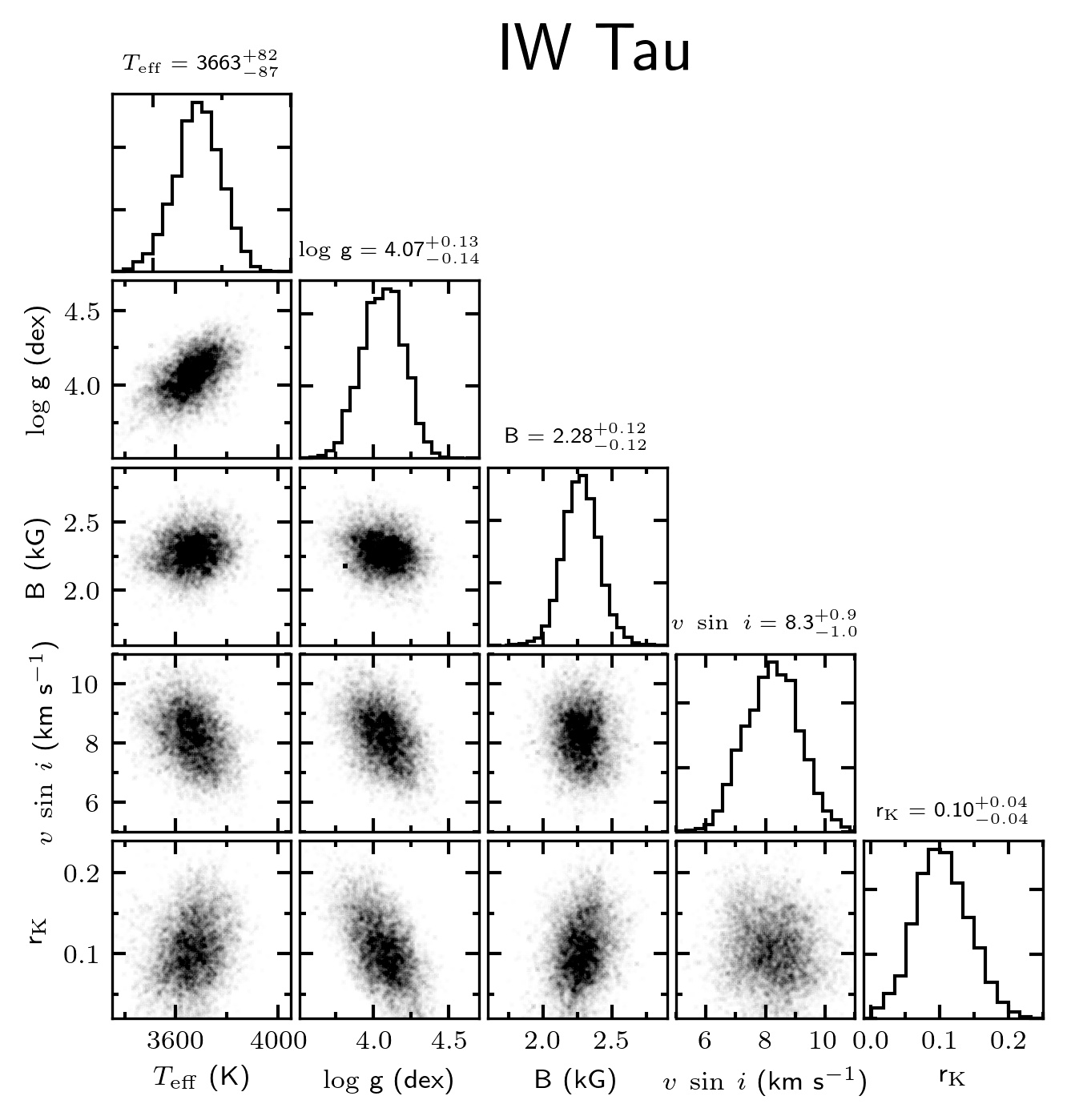
In Figure 3, we show the posterior distributions of the MCMC analysis for the star IW Tau as an illustrative example. Figure 3 also shows the dependence between stellar parameters like g and rK. A good fit to the observation can be achieved with a slightly lower g , or a higher rK because both g or veiling varies the CO line depths. The degeneracy between these parameters adds to the uncertainty in each quantity separately.
III.4 Uncertainties
The 16th and 84th percentiles of the posterior probability distributions of the stellar parameters represent the formal uncertainties of our fitting method. Most of the uncertainties were found to be nearly symmetric, and we report the larger of the two percentiles as the corresponding symmetric uncertainty () for each parameter. The median fit uncertainties are 152 K in , 0.25 dex in g, 0.54 kG in B, 1.9 km s-1 in , and 0.10 in rK.
Additionally, we quantified the systematic uncertainties () by comparing our stellar parameters to previously published values. Stars with precise physical parameters provided by interferometric observations help mitigate model dependency by calibrating relationships between and stellar radius. The works of Mann et al. 2013; Mann et al. 2015 and Newton et al. 2015 used 20 stars with interferometric measurements to calibrate their model-independent relationships with 150 K precision. To quantify the for and g, we determined the stellar parameters of seven field M stars with metallicity close to the solar value ([Fe/H]=0.00.10 dex) from Mann et al. 2013.
We used the same fitting routines as for the YSO sample, but assuming rK = 0.0 since these stars are on the main sequence and diskless. In Table 2, we compared our and g values with those obtained by Mann et al. 2013. They determined , [Fe/H], mass (M) and radius (R), which we used in the following equation to compute their g values:
| (2) |
| 2MASS ID | Alt. Name | K | SpT | Class | Ref | Binary | Ref | N | SNRK | flag | g | B | |||
|---|---|---|---|---|---|---|---|---|---|---|---|---|---|---|---|
| (mag) | (K) | (dex) | (kG) | (km s-1) | |||||||||||
| J04141760+2806096 | [BCG93] 1 | 9.9 | M5.0 | II | 1,2,3,4 | ? | – | 2 | 172 | 0 | 3281197 | 3.880.40 | 1.09 | 9.92.9 | 1.100.21 |
| J05075496+2500156 | [BCG93] 12 | 10.4 | M3.7 | II | 2,4 | N | 16 | 2 | 64 | 3 | |||||
| J04182909+2826191 | [SS94] V410 Anon 25 | 9.9 | M3.5 | III | 2,4,5 | ? | – | 1 | 87 | 1 | 3619328 | 4.050.59 | 2.32 | 30.77.4 | 0.390.20 |
| J04174965+2829362 | [SS94] V410 X-ray 1 | 9.1 | M3.7 | II | 2,3,4 | N | 16 | 2 | 182 | 0 | 3315129 | 3.370.25 | 1.220.33 | 9.72.0 | 0.280.06 |
| J04183444+2830302 | [SS94] V410 X-ray 2 | 9.2 | M0.0 | II | 2,4 | ? | – | 2 | 182 | 0 | 4231143 | 4.530.27 | 1.840.49 | 10.92.9 | 0.440.08 |
| J04345542+2428531 | AA Tau | 8.0 | M0.6 | II | 1,2,3,4 | N | 16 | 10 | 356 | 0 | 3751171 | 3.870.26 | 2.160.41 | 12.52.3 | 1.560.12 |
| J04191583+2906269 | BP Tau | 7.7 | M0.5 | II | 1,2,3,4 | N | 16 | 7 | 353 | 0 | 3719131 | 4.010.25 | 2.190.37 | 9.92.3 | 1.360.11 |
| J04335200+2250301 | CI Tau | 7.8 | K5.5 | II | 2,3,4 | N | 16 | 10 | 931 | 0 | 395194 | 3.770.17 | 1.950.31 | 12.51.9 | 2.340.09 |
| J04265440+2606510 | CoKu FV Tau c | 8.9 | M2.5 | II | 1,2,3,4 | Y | 24 | 6 | 302 | 0 | 3456136 | 3.530.23 | 2.01 | 38.62.4 | 0.330.06 |
| J04355349+2254089 | CoKu HP Tau G3 | 8.8 | M0.6 | III | 1,2,3,4,5 | Y | 16 | 6 | 239 | 0 | 3760164 | 3.840.26 | 2.65 | 43.32.9 | 0.250.07 |
| J04354093+2411087 | CoKu Tau 3 | 8.4 | M0.5 | II | 1,2,3,4 | N | 16 | 5 | 249 | 0 | 3665154 | 3.850.26 | 2.330.34 | 8.22.1 | 0.770.08 |
| J04411681+2840000 | CoKu Tau 4 | 8.7 | M1.1 | II | 1,2,4 | Y | 13 | 6 | 254 | 0 | 3706121 | 3.700.21 | 1.90 | 26.32.2 | 0.220.04 |
| J04144786+2648110 | CX Tau | 8.8 | M2.5 | II | 1,2,3,4 | N | 16 | 2 | 152 | 0 | 3520180 | 3.610.30 | 1.39 | 20.52.5 | 0.280.08 |
| J04173372+2820468 | CY Tau | 8.6 | M2.3 | II | 1,2,3,4 | N | 16 | 2 | 203 | 0 | 3445155 | 3.730.28 | 1.31 | 10.82.3 | 0.810.13 |
| J04183158+2816585 | CZ Tau | 9.4 | M4.2 | II | 1,2,3,4 | Y | 18 | 4 | 220 | 1 | 3385211 | 3.830.35 | 1.70 | 31.43.1 | 0.640.12 |
| J04183112+2816290 | DD Tau | 7.9 | M3.5 | II | 1,2,3,4 | Y | 6 | 4 | 251 | 0 | 3250207 | 3.470.37 | 1.48 | 16.93.1 | 1.820.26 |
| J04215563+2755060 | DE Tau | 7.8 | M2.3 | II | 1,2,3,4 | N | 16 | 4 | 251 | 0 | 3463158 | 3.450.27 | 1.01 | 9.42.2 | 1.110.11 |
| J04270280+2542223 | DF Tau | 6.7 | M2.0 | II | 1,2,3,4 | Y | 24 | 4 | 293 | 3 | |||||
| J04270469+2606163 | DG Tau | 7.0 | K7.0 | II | 1,2,3,4 | N | 16 | 5 | 553 | 2 | 3969216 | 3.200.28 | 1.78 | 26.94.3 | 4.820.94 |
| J04294155+2632582 | DH Tau | 8.2 | M2.3 | II | 1,2,3,4 | N | 16 | 10 | 399 | 0 | 3477125 | 3.890.22 | 2.210.32 | 8.42.1 | 1.240.10 |
(1)Kenyon & Hartmann 1995; (2)Luhman et al. 2010; (3)Rebull et al. 2010; (4)Esplin et al. 2014; (5)Kraus et al. 2017; (6)Bouvier et al. 1992; (7)Correia et al. 2006; (8)Duchêne et al. 1999; (9)Dyck et al. 1982; (10)Ghez et al. 1993; (11)Haas et al. 1990; (12)Herbig & Bell 1988; (13)Ireland & Kraus 2008; (14)Konopacky et al. 2007; (15)Kraus et al. 2006; (16)Kraus et al. 2011; (17)Leinert et al. 1991; (18)Leinert et al. 1993; (19)Mathieu et al. 1991; (20)Mathieu et al. 1996; (21)Richichi et al. 1999; (22)Ruíz-Rodríguez et al. 2016; (23)Schaefer et al. 2014; (24)Simon et al. 1992; (25)Walter et al. 1988; (26)Weintraub 1989.
We found an average difference in g (ours - Mann) of 0.04 dex and a standard deviation of the residuals of 0.13 dex. For we found a mean difference of -69 K and a standard deviation of the residuals of 75 K. Therefore, we assigned 0.13 dex and 75 K as the systematic uncertainties for g and , respectively.
To obtain the systematic uncertainty on , we compared measurements for 52 YSOs in common with Nofi et al. 2021. In that work, they determined the of pre-main-sequence stars using the same single-epoch, uncombined IGRINS K-band spectra that we have used. Their method used the cross-correlation technique outlined in Hartmann et al. 1986 and Soderblom et al. 1989 along with synthetic spectra. In brief, a stellar spectrum with rotationally broadened lines was cross-correlated against an unbroadened spectrum. Then the width of the cross-correlation function is used to measure the rotational broadening of the spectrum. Generally, our values were in good agreement with those of Nofi et al. 2021. We found a mean difference between the values (ours - Nofi) of 0.2 km s-1 and a standard deviation of the residuals of 1.7 km s-1. We assigned this 1.7 km s-1 as the systematic uncertainty.
Over 85% of our values are 30 km s-1, with the median value being 16.6 km s-1. In Figure 4 we compare measurements for 60 YSOs in common with Nguyen et al. 2012. They used high-resolution (R=60,000) optical (4800–9300 Å) spectra to determine for pre-main-sequence stars in the Chamaeleon i and Taurus-Auriga star-forming regions. Their method compared each echelle order of the target spectrum with slow-rotating template stars, which were artificially broadened to different values of to find the best fit. Finally, they removed 2.7 outliers around the mean value and computed a weighted average over all the remaining echelle orders (Nguyen et al. 2009, for more details see also). We found our values in agreement with those of Nguyen et al. 2012, with an mean difference of 0.08 km s-1, and a error on the mean of 0.3 km s-1.

Finally, we collected 12 determinations (for 11 YSOs) of B-field strength from the literature (Johns-Krull 2007; Sokal et al. 2020; Flores et al. 2020) to assess the systematic uncertainty of our B values (see Table 3). We found a mean difference in the residuals (ours - literature) of kG and a standard deviation of 0.26 kG. We assigned 0.26 kG as our systematic uncertainty in the B-field measurements.
The systematic uncertainties were added in quadrature to the fit errors to compute the total error of each parameter (), which we report in Table 1.
| Mann et al. 2013 | this work | |||
|---|---|---|---|---|
| Star | g | g | ||
| (K) | (dex) | (K) | (dex) | |
| GJ 338A | 395341 | 4.710.05 | 381356 | 4.680.09 |
| GJ 338B | 392637 | 4.720.04 | 378554 | 4.690.08 |
| GJ 436 | 352066 | 4.770.06 | 358759 | 4.900.11 |
| GJ 570A | 458858 | 4.570.07 | 453650 | 4.360.11 |
| GJ 702B | 447533 | 4.660.04 | 439138 | 4.500.14 |
| GJ 809 | 374427 | 4.720.04 | 360463 | 4.590.09 |
| GJ 887 | 369535 | 4.780.05 | 369967 | 4.950.08 |
| Star | B literature | Ref. | B this work |
|---|---|---|---|
| (kG) | (kG) | ||
| AA Tau | 2.780.28 | JK07 | 2.160.32 |
| BP Tau | 2.170.22 | JK07 | 2.190.27 |
| BP Tau | 2.500.16 | F19 | 2.190.27 |
| CI Tau | 2.150.15 | S20 | 1.950.16 |
| CY Tau | 1.160.12 | JK07 | 1.310.37 |
| DE Tau | 1.120.11 | JK07 | 1.010.24 |
| DH Tau | 2.680.27 | JK07 | 2.210.18 |
| DK Tau | 2.640.26 | JK07 | 2.550.58 |
| DN Tau | 2.000.20 | JK07 | 1.540.26 |
| GI Tau | 2.730.27 | JK07 | 1.920.36 |
| GK Tau | 2.280.23 | JK07 | 2.050.87 |
| GM Aur | 2.220.22 | JK07 | 2.110.22 |
IV Results and analysis

We plotted the spectral regions used in our analysis for all the observed and the best-fit spectra, as in Figure 5, to categorize the quality of our parameter determinations. Through a ranking of the statistics and visual inspection, we marked each set of parameters in Table 1 with a numerical flag equal to 0, 1, or 3 if they are good, acceptable, or poor determinations, respectively. We also computed the lower and upper limits of each parameter using its total uncertainty, to look for values outside or at the edge of our grid. We find that six lower limits of g meet this criterion. We flagged these parameters with a flag equal to 2 and have retained these measurements in our analysis since they are otherwise classified as ‘good’ determinations. We found that our parameter determination method needs a minimum median SNR 80 to produce reliable results. A median SNR 150 is generally required for good parameter determinations. In total, we identified 80, 24, 9, and 6 stars whose parameters are good, acceptable, poor, and outside/edge of grid, respectively. We exclude poor determinations in further analysis, and we will refer to the 110 remaining YSO measurements as our Taurus sample.
IV.1 Magnetic fields
While Zeeman line splitting effects are most significant in the Ti region, the Na region is also sensitive to variations in the B field (see Figure 2). However, our ability to measure Zeeman line separations is primarily a function of the line widths, which are dominated by . Hussaini et al. 2020 measured the line splitting of the Na and Ti spectral regions in IGRINS data and the moogstokes spectra employed in this work. That work found that the retrieval of B is limited to /10 in the Ti region and /5 in the Na region. In other words, an object with = 15 km s-1 must have B 1.5 kG for Zeeman splitting to be measurable in the Ti region and 3 kG to be measurable in the Na region. Additionally, the IGRINS spectral resolution limits the minimum measurable B field from line splitting to 0.7 kG. For this work, we conservatively considered a detection limit of B (/8) kG, and no lower than 1 kG. Values of B field lower than 1 kG can not be distinguished from a non-detection at the spectral resolution of IGRINS when simultaneously fitting for other model parameters. We found that 41 of our B field determinations meet the detection threshold. The remaining upper-limit measurements are provided in Table 1.
IV.2 Impact of B on the stellar parameters

To evaluate the impact of B on , g, , and , we fixed B to 0 kG and redetermined the stellar parameters for the 41 YSOs with B-field detections in Table 1. In Figure 6 we compare the stellar parameters determined in our primary analysis with those obtained by disabling the B parameter. We further consider the low B (objects with B 2 kG) and the high B (B 2 kG) results in this comparison.
We found that all the values determined without considering the B-field effects are systematically colder than those found considering the B-field. For low B (18 objects), we found a mean difference of 424 K, while for high B (23 objects), this difference increases slightly to 739 K. Both values are well within the median total (fit+systemic) error, which is 170 K. Similarly, rK is lower when B is not taken into account, with a mean difference of 0.140.02 for both the low and high B bins. Contrary to and rK, most of the g values are higher by 0.080.01 dex and 0.030.01 dex for the low and high B bins, respectively, when not considering B-fields in the fit. These g differences are within the g median total (fit+systemic) error of 0.28 dex. It is likely that the degeneracy between g and discussed in Section III.3 is why g is overestimated and is underestimated when B is not included in the parameter determinations.
The most prominent effect of ignoring the B-field strength when determining parameters is seen in the values. All determinations are higher without B-field included in the fit, and the difference is greater for larger values of B. We found for the low-B bin a mean difference of 1.60.2 km s-1. For the high-B bin, the difference increases to 3.80.3 km s-1. This trend is explained by excess rotational broadening of the synthetic spectral lines to try and replicate the B-field induced Zeeman line-splitting. The absence of B-field considerations by Nguyen et al. 2012 and Nofi et al. 2021 is likely responsible for some of the differences between those works and ours, which adds to the systematic uncertainties.
The previous tests suggest that it is possible to obtain suitable stellar parameters, even when excluding the B-field from the determination. However, the parameters will have systematic offsets, with magnetically active YSO parameters being the most impacted.
IV.3 Effective Temperature

Kenyon & Hartmann 1995 presented a conversion between spectral type and for young stars, based on the work of Schmidt-Kaler 1982 and Straižys 1992. Shortly after, Luhman 1999 developed a new temperature scale for young M stars between the giant and dwarf scales. However, improvements made in the last two decades in the modeling of cool star atmospheres, and the development of new instruments, have resulted in several studies that have determined effective temperatures (or spectral type) either for field (e.g., Casagrande et al. 2008; Rajpurohit et al. 2013; Rajpurohit et al. 2018; López-Valdivia et al. 2019) or for young (e.g., Luhman et al. 2003a; Luhman et al. 2003b; Herczeg & Hillenbrand 2014; Cottaar et al. 2014; Yao et al. 2018) K & M stars.
In Figure 7 we compare the values we determined to spectral types from Luhman et al. 2017, along with three different temperature scales of pre-main-sequence stars (Luhman et al. 2003b; Herczeg & Hillenbrand 2014; Pecaut & Mamajek 2013). To analyze how multiplicity plays a role in determining , we divided our sample into single (51) and binary (44) stars based on classifications from the literature. These identifications are reported in Table 1. We consider a star a binary if it has a companion closer than 2 arcseconds because the resultant IGRINS spectrum will contain some amount of flux from both components.
The amount of contamination from a binary companion is not easily quantified. An equal brightness binary with no velocity offsets will have composite line profiles, often producing poor fits to the data. If the binary has equal brightness and radial velocity offsets (a double-lined spectroscopic binary), then line blending in the combined spectrum will often result in poor parameter determinations. Generally, equal brightness binaries have been excluded from our analysis by visual inspection in the initial sample selection and at the parameter-fit quality check. Binaries with disproportionate fluxes will have the same issues as the equal flux binaries, but at lower levels. Stellar parameters obtained for the known binary stars should be used with caution since secondary contamination is possible, although the spectral fit is dominated by the primary star’s contribution. The binary identification here allows us to look for systematic differences in the data.
In general our temperatures follow the scales of Pecaut & Mamajek 2013, Herczeg & Hillenbrand 2014 and Luhman et al. 2003b for both the single and binary samples. Early K-type binaries (T Tau, RW Aur, and HQ Tau) show large discrepancies which is possibly due to wrong SpT classifications, as Flores et al. 2020 also found a cooler temperature for T Tau (=397690 K), cool spots or the binary nature of these YSOs biasing measurements to cooler temperatures. A more detailed multi-epoch and multi-wavelength study should be carried out at higher angular resolution to understand the large variation in temperatures for these early-K binaries.
A temperature scale for the single stars was computed using the mean value and the standard deviation within 0.5 spectral type sub-classes bins. This IGRINS temperature scale, reported in Table 4, represents an alternative to previous published pre-main-sequence stars temperature scales, with the advantage of being obtained through a simultaneous determination of various atmospheric parameters and the inclusion of the magnetic field effects.
| SpT | L03 | PM13 | HH14 | This work | N |
|---|---|---|---|---|---|
| (K) | (K) | (K) | (K) | ||
| K0 | – | 5030 | 4870 | 4606233 | 1 |
| K2 | – | 4760 | 4710 | 4450123 | 1 |
| K5 | – | 4140 | 4210 | 405578 | 2 |
| K7 | – | 3970 | 4020 | 390563 | 2 |
| M0 | – | 3770 | 3900 | 3769111 | 5 |
| M1 | 3705 | 3630 | 3720 | 369656 | 9 |
| M2 | 3560 | 3490 | 3560 | 353579 | 9 |
| M3 | 3415 | 3360 | 3410 | 349626 | 5 |
| M4 | 3270 | 3160 | 3190 | 331958 | 3 |
| M5 | 3125 | 2880 | 2980 | 326948 | 2 |
IV.4 Surface gravity, stellar ages and masses
The g– plane, also known as the spectroscopic Hertzsprung-Russell diagram (Langer & Kudritzki 2014, sHR;), helps estimate stellar properties such as age and mass because g and are proxies for those properties (Sokal et al. 2018, See Figure 9 of). According to the evolutionary models of Baraffe et al. 2015, over the mass range of 0.05–1.4 , the g changes by about 0.5 dex between 1 to 10 Myr. Therefore, two populations of different ages should occupy different parts of the sHR.
With this in mind, we observed members of the TW Hydrae Association (TWA; Kastner et al. 1997). TWA is a nearby (60 pc; Zuckerman & Song 2004; Gaia Collaboration et al. 2018) and young (7–10 Myr; Ducourant et al. 2014; Herczeg & Hillenbrand 2015; Sokal et al. 2018) group of stars, that serves as an evolved counterpart to our Taurus sample. We analyzed and determined the stellar parameters (Table 5) for all 19 TWA objects in the same fashion as the Taurus sample. In Figure 8 we assemble the sHR of the Taurus and TWA YSOs, and compare them to the 1, 5, and 10 Myr isochrones of Baraffe et al. 2015.
| 2MASS ID | Name | SpT | Ref. | K | flag | g | B | |||
|---|---|---|---|---|---|---|---|---|---|---|
| (mag) | (K) | (dex) | (kG) | (km s-1) | ||||||
| J11015191-3442170 | TWA 1 | M0.5 | 1 | 7.3 | 0 | 3783108 | 4.350.18 | 2.750.30 | 8.42.0 | 0.530.05 |
| J11091380-3001398 | TWA 2 | M2.2 | 1 | 6.7 | 0 | 3558 92 | 4.070.16 | 1.38 | 15.91.9 | 0.060.02 |
| J11102788-3731520 | TWA 3A | M4.1 | 1 | 6.8 | 1 | 3285 75 | 4.000.13 | 0.97 | 11.91.7 | 0.290.01 |
| – | TWA 3B | M4.0 | 1 | – | 1 | 3355 75 | 4.200.13 | 1.78 | 15.81.7 | 0.160.01 |
| J11220530-2446393 | TWA 4 | K6.0 | 1 | 5.6 | 0 | 4257103 | 4.510.21 | 1.10 | 10.22.1 | 0.310.04 |
| J10423011-3340162 | TWA 7 | M3.2 | 1 | 6.9 | 0 | 3328 80 | 4.270.13 | 2.190.26 | 7.41.7 | 0.100.01 |
| J11324124-2651559 | TWA 8A | M2.9 | 1 | 7.4 | 0 | 3398 75 | 4.300.13 | 2.860.26 | 7.51.7 | 0.130.01 |
| J11482422-3728491 | TWA 9A | K6.0 | 1 | 7.8 | 0 | 4043 94 | 4.320.17 | 2.290.30 | 12.02.0 | 0.170.03 |
| J11482373-3728485 | TWA 9B | M3.4 | 1 | 9.2 | 0 | 3351 75 | 4.300.14 | 1.30 | 10.91.7 | 0.090.01 |
| J12350424-4136385 | TWA 10 | M3.0 | 2 | 8.2 | 1 | 3358 75 | 4.230.13 | 2.540.26 | 9.51.7 | 0.100.01 |
| J12360055-3952156 | TWA 11B | M2.5 | 3 | 8.3 | 0 | 3532115 | 4.220.18 | 2.230.34 | 14.82.1 | 0.020.02 |
| 12354893-3950245, | TWA 11C | M4.5 | 2 | 8.9 | 1 | 3391122 | 4.450.22 | 1.98 | 22.82.3 | 0.360.04 |
| J11210549-3845163 | TWA 12 | M2.75 | 2 | 8.1 | 0 | 3534104 | 4.190.17 | 2.670.32 | 19.72.0 | 0.020.02 |
| J11211723-3446454 | TWA 13A | M1.1 | 1 | 7.5 | 0 | 3638 96 | 4.140.16 | 2.120.29 | 14.21.9 | 0.040.02 |
| J11211745-3446497 | TWA 13B | M1.0 | 1 | 7.5 | 0 | 3673 93 | 4.130.16 | 1.710.30 | 13.71.9 | 0.040.02 |
| J12345629-4538075 | TWA 16 | M3.0 | 2 | 8.1 | 0 | 3445 91 | 4.150.16 | 1.850.28 | 12.41.9 | 0.070.02 |
| J12072738-3247002 | TWA 23 | M3.5 | 1 | 7.8 | 1 | 3405101 | 4.150.18 | 1.42 | 19.11.9 | 0.160.03 |
| J12153072-3948426 | TWA 25 | M0.5 | 1 | 7.3 | 0 | 3707 99 | 4.140.17 | 2.210.29 | 15.01.9 | 0.060.03 |
| J10120908-3124451 | TWA 39 | M4.0 | 4 | 8.0 | 1 | 3316 88 | 4.060.18 | 1.34 | 18.02.0 | 0.280.03 |
(1) Herczeg & Hillenbrand 2014; (2) Luhman et al. 2017; (3) Webb et al. 1999; (4) Riedel et al. 2014

As expected, the Taurus and TWA YSOs populate different parts of the sHR, exhibiting an offset in g. Most of the Taurus sample is located between the 1 and 5 Myr isochrones while the TWA members are located below the 5 Myr isochrone. We found a mean g (and error on the mean) of 3.870.03 dex and 4.220.03 dex, for Taurus and TWA, respectively.
We applied to the g distributions of Taurus and TWA a Kolmogorov-Smirnov (KS) test55 5 We have used the KS_2samp function, which is part of the python package Scipy.stats. The KS test explores the null hypothesis that two samples are drawn from the same distribution. If the probability value () obtained from this test is higher than a certain threshold, often set at 1%, 5%, or 10%, we cannot reject the null hypothesis. We found a that the g distributions of Taurus and TWA come from the same parent distribution, validating that precise g values can provide meaningful age proxies for populations of stars.
For the mean and g values, and the set of isochrones from Baraffe et al. 2015, we can make a rough estimate of the age of Taurus and TWA. Our calculations lead to a Taurus mean age of 2.5 Myr and a TWA mean age of 10 Myr. However, the dispersion within these groups is larger than the differences between them. The parameters of the least evolved TWA members are more similar to the more evolved members of Taurus than to the most evolved members of TWA.
IV.5 Class ii vs. Class iii YSOs
Based on the shape of their spectral energy distributions, Adams et al. 1987 divided YSOs into three different morphological classes (i, ii, and iii) using the spectral index , and suggested that such classes represent an evolutionary sequence in the formation of low-mass stars. Since then, the sequence has been extended to Class 0 YSOs embedded in an infalling cold dust envelope (Andre et al. 1993), flat spectrum YSOs (Greene et al. 1994) between Class i and ii, and post-Class iii transition disk objects without the cold dust corresponding to flux from 5-20 m (Lada et al. 2006). If the classification of YSOs by their SED slope, as suggested, represents an evolutionary scheme, the populations of YSOs would differ in terms of stellar properties, such as g, given that stars undergo gravitational contraction while they evolve towards the main-sequence (Herbig 1962).
To test this, we collected YSO classifications from the literature for 84 Class ii and 35 Class iii (78 and 32 with good or acceptable parameters, respectively) objects in our sample (Kenyon & Hartmann 1995; Luhman et al. 2010; Rebull et al. 2010; Esplin et al. 2014; Kraus et al. 2017). We used a KS test to quantify if the stellar parameters determined for the Class ii and Class iii stars are statistically different.
We found a (KS) of 32%, 9%, and 6% that the Class ii and Class iii objects come from the same parent distributions of , , and B respectively.66 6 We considered just the 41 B determinations in this test, not the limits. This probability dropped to values lower than 1% for g and . These probability values indicate that the Class ii and Class iii YSOs of our sample are statistically indistinguishable in terms of , marginally indistinguishable in terms of and B, but different in terms of and g.
The result of the KS tests for and are not surprising. The distribution of temperatures (SpT) reflects the initial mass function of Taurus. Also, Class ii YSOs host disks and are actively accreting, which correlate with high levels of veiling, while Class iii objects have lost their disks and show little or no veiling. The veiling values we measure for Class iii objects is closer to zero than what we find for Class ii YSOs, consistent with the expected behavior. For , the (KS) of 9% that we found is in agreement with the findings of Nguyen et al. 2009, who found that low-mass accretors and non-accretors in Taurus have a (KS) = 10% of coming from the same parent distribution.
Since g can be used as a proxy for age (Yao et al. 2018), the different distributions for Class ii and Class iii YSOs support the idea of an evolutionary sequence (see Figure 9). We found a mean g of 3.830.03 and 4.060.04 dex for Class ii and Class iii Taurus objects, respectively. The most interesting sources in each g distribution are those in the wings, where evolutionary differences between the lowest g Class iii YSOs and the highest g Class ii YSOs are still not well understood.
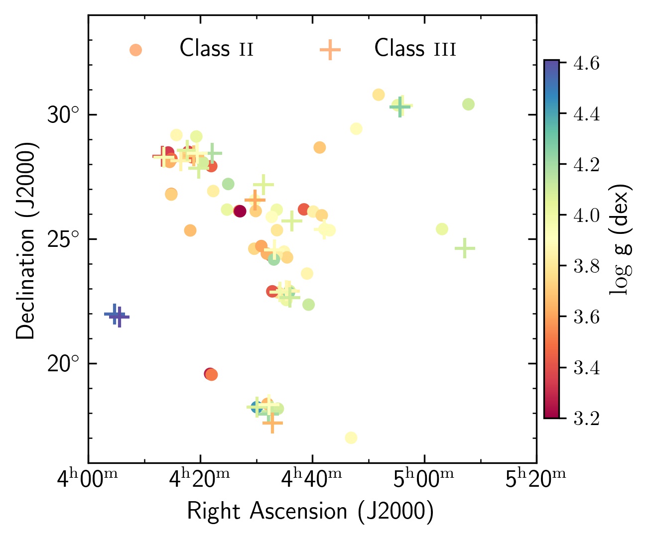
Finally, the spatial distribution for the IGRINS Taurus sample (Figure 10) does not show significant clustering of Class ii or Class iii objects, nor a trend with g, suggesting that there is not a star formation gradient across the cloud. Yet, this is a 2-dimensional view of Taurus, and it will require the entire population of Taurus YSOs (Luhman 2018, 400;) studied in the context of 3-dimensional substructures (Krolikowski et al. 2021) before we can fully understand the spatial distribution in relation to the parameters we have determined.

IV.6 Important Considerations
There are many ways to perform the parameter determination that we present here.
As outlined above, there are a variety of models to choose from and possible approaches.
We have shown that magnetic fields are a critical component of the parameter determination, and we allowed many of the YSO parameters to remain variables in the fit rather than fixing them to assumed values.
During our tests, we found that g was the most sensitive parameter to variations in our approach.
Additionally, we fit for all parameters simultaneously rather than taking an iterative approach to the fitting.
While deciding on the best method for parameter determination, by minimizing fit residuals and validating the results against the literature, we have identified some important considerations when performing YSO parameter determinations.
Use of consistent estimators: IGRINS provides us with both the H- and K-band spectrum of our sources, but we have only employed the K-band in our analysis.
There are temperature sensitive spectral features in the H-band (the OH region of López-Valdivia et al. 2019) that we initially included in our analysis.
The result of including this H-band region was an offset in g towards higher values, inconsistent with the evolutionary stage of the Taurus star-forming region.
Using both the H- and K-band spectra meant that g came primarily from the CO region and came from the OH region, which are about 0.7 m apart.
Furthermore, Gully-Santiago et al. 2017 found that varies as a function of wavelength when a single temperature component was fit to the IGRINS spectrum of the spotted YSO LkCa 4. The temperature in the CO region of LkCa 4 is 700 K cooler than the value determined in the OH region (see Figure 3 of Gully-Santiago et al. 2017).
In this work, differences between the H- and K-band temperatures were compensated for by the remaining stellar parameters, which primarily impacted the g determination.
While the broad spectral grasp of IGRINS permits the analysis of additional features, it also probes different components of the YSO photosphere, which can produce conflicting measurements.
We have mitigated these effects by fitting only the K-band regions of the Taurus YSOs.
Degeneracy between and g: Another consideration was the degeneracy between g and . As seen in the diagonal distribution of and g in the sub-panel of Figure 3, higher values of results in lower g values, and vice versa. This degeneracy results at a fixed because and g impact the CO lines in nearly in the same way, and the CO lines are the most g sensitive lines in our analysis.
This degeneracy increases the uncertainties for each parameter and we concluded that g and need to be determined simultaneously and from the same spectrum.
The use of fixed or g values from the literature will disproportionately impact the other parameter.
The atomic data: Our method relies on the comparison of observed and synthetic spectra, and the line list and the model atmosphere selected is a crucial component of the result.
We initially determined the stellar parameters using the unmodified VALD line list expecting that the use of different spectral regions would average the inaccuracies of the atomic data.
However, the resultant stellar parameters were offset from previous determinations in the literature.
We then modified the oscillator strengths and the van der Wals constants of our spectral regions to the values of Flores et al. 2019, which improved the stellar parameter determinations and the consistency with the literature.
We used the Flores et al. 2019 modifications because they were obtained from spectra with a spectral resolution close to IGRINS and for the same spectral regions we have employed.
Comparison with the literature: The bright YSOs in this work are canonical members of the Taurus-Auriga star forming region and have numerous published parameters. Many of the prior works in the literature (Johns-Krull 2007; Pecaut & Mamajek 2013; Herczeg & Hillenbrand 2014, e.g.,) fixed parameters that we have left as variables in the fits. Prior studies also analyzed shorter wavelength regions of the YSO spectra, which are dominated by the hotter photosphere. Additionally, the variable nature of YSOs means that observations made at different epochs likely have different physical properties. In comparing our results to the literature, we find that the observed spectra and methods of Flores et al. 2019 provide the most direct comparisons and consistency.
V Summary and conclusions
We employed four different spectral regions of the infrared K-band and an iterative MCMC approach to determine , g, B, and for a sample of canonical YSOs in the Taurus-Auriga star-forming region. Our analyses used a solar metallicity synthetic spectral grid of MARCS atmosphere models and the spectral synthesis code moogstokes. Our observational data were obtained with the Immersion GRating INfrared Spectrometer (IGRINS).
We were able to reliably determine , g, and for 110 YSOs. Our ability to determine B is dependent on the and limited by the spectral resolution of IGRINS. We established that B values 1 kG or (/8) kG are required to provide meaningful B-field detections, and that SNR150 is desirable for overall parameter fitting. Measurable B-fields were found for 41 of the YSOs, and upper limits were identified for the remaining objects.
The we derived agrees with previous temperature scales for spectral type M YSOs, but it is systematically cooler for K stars. This could be a result of the models used in this analysis compared to others or the wavelength regions studied, which are more sensitive to the cool spotted regions of hotter YSOs. Our results show that the Class ii and Class iii objects are statistically similar in terms of , marginally similar in and B, and different in g and rK. The differences found in the distributions of g and rK correspond to the expected behavior if Class iii are more evolved than Class ii objects. We found mean g values of 3.830.03, 4.060.04, and 4.220.03 dex for the Taurus Class ii and Class iii objects and 19 TWA members, respectively. These differences are statistically significant and affirms the age gradient between these young star populations.
References
- Adams et al. (1987) Adams, F. C., Lada, C. J., & Shu, F. H. 1987, ApJ, 312, 788
- ALMA Partnership et al. (2015) ALMA Partnership, Brogan, C. L., Pérez, L. M., et al. 2015, ApJ, 808, L3
- Andre et al. (1993) Andre, P., Ward-Thompson, D., & Barsony, M. 1993, ApJ, 406, 122
- Astropy Collaboration et al. (2013) Astropy Collaboration, Robitaille, T. P., Tollerud, E. J., et al. 2013, A&A, 558, A33
- Astropy Collaboration et al. (2018) Astropy Collaboration, Price-Whelan, A. M., Sipőcz, B. M., et al. 2018, AJ, 156, 123
- Attridge & Herbst (1992) Attridge, J. M., & Herbst, W. 1992, ApJ, 398, L61
- Baraffe et al. (2015) Baraffe, I., Homeier, D., Allard, F., & Chabrier, G. 2015, A&A, 577, A42
- Barenfeld et al. (2017) Barenfeld, S. A., Carpenter, J. M., Sargent, A. I., Isella, A., & Ricci, L. 2017, ApJ, 851, 85
- Baruteau et al. (2014) Baruteau, C., Crida, A., Paardekooper, S. J., et al. 2014, in Protostars and Planets VI, ed. H. Beuther, R. S. Klessen, C. P. Dullemond, & T. Henning, 667
- Basri & Batalha (1990) Basri, G., & Batalha, C. 1990, ApJ, 363, 654
- Basri & Bertout (1989) Basri, G., & Bertout, C. 1989, ApJ, 341, 340
- Bean et al. (2006) Bean, J. L., Sneden, C., Hauschildt, P. H., Johns-Krull, C. M., & Benedict, G. F. 2006, ApJ, 652, 1604
- Boccaletti et al. (2020) Boccaletti, A., Di Folco, E., Pantin, E., et al. 2020, A&A, 637, L5
- Bouvier et al. (2014) Bouvier, J., Matt, S. P., Mohanty, S., et al. 2014, in Protostars and Planets VI, ed. H. Beuther, R. S. Klessen, C. P. Dullemond, & T. Henning, 433
- Bouvier et al. (1992) Bouvier, J., Tessier, E., & Cabrit, S. 1992, A&A, 261, 451
- Calvet et al. (1984) Calvet, N., Basri, G., & Kuhi, L. V. 1984, ApJ, 277, 725
- Camenzind (1990) Camenzind, M. 1990, Reviews in Modern Astronomy, 3, 234
- Casagrande et al. (2008) Casagrande, L., Flynn, C., & Bessell, M. 2008, MNRAS, 389, 585
- Cieza et al. (2005) Cieza, L. A., Kessler-Silacci, J. E., Jaffe, D. T., Harvey, P. M., & Evans, Neal J., I. 2005, ApJ, 635, 422
- Correia et al. (2006) Correia, S., Zinnecker, H., Ratzka, T., & Sterzik, M. F. 2006, A&A, 459, 909
- Cottaar et al. (2014) Cottaar, M., Covey, K. R., Meyer, M. R., et al. 2014, The Astrophysical Journal, 794, 125
- Crockett et al. (2012) Crockett, C. J., Mahmud, N. I., Prato, L., et al. 2012, ApJ, 761, 164
- Cutri et al. (2003) Cutri, R. M., Skrutskie, M. F., van Dyk, S., et al. 2003, VizieR Online Data Catalog, II/246
- Deen (2013) Deen, C. P. 2013, AJ, 146, 51
- Doppmann et al. (2003) Doppmann, G. W., Jaffe, D. T., & White, R. J. 2003, AJ, 126, 3043
- D’Orazi et al. (2011) D’Orazi, V., Biazzo, K., & Randich, S. 2011, A&A, 526, A103
- Duchêne et al. (1999) Duchêne, G., Monin, J. L., Bouvier, J., & Ménard, F. 1999, A&A, 351, 954
- Ducourant et al. (2014) Ducourant, C., Teixeira, R., Galli, P. A. B., et al. 2014, A&A, 563, A121
- Dyck et al. (1982) Dyck, H. M., Simon, T., & Zuckerman, B. 1982, ApJ, 255, L103
- Esplin et al. (2014) Esplin, T. L., Luhman, K. L., & Mamajek, E. E. 2014, ApJ, 784, 126
- Fischer et al. (2011) Fischer, W., Edwards, S., Hillenbrand, L., & Kwan, J. 2011, ApJ, 730, 73
- Flores et al. (2019) Flores, C., Connelley, M. S., Reipurth, B., & Boogert, A. 2019, ApJ, 882, 75
- Flores et al. (2020) Flores, C., Reipurth, B., & Connelley, M. S. 2020, arXiv e-prints, arXiv:2006.10139
- Foreman-Mackey et al. (2013) Foreman-Mackey, D., Hogg, D. W., Lang, D., & Goodman, J. 2013, PASP, 125, 306
- Gahm et al. (2008) Gahm, G. F., Walter, F. M., Stempels, H. C., Petrov, P. P., & Herczeg, G. J. 2008, A&A, 482, L35
- Gaia Collaboration et al. (2018) Gaia Collaboration, Brown, A. G. A., Vallenari, A., et al. 2018, A&A, 616, A1
- Galli et al. (2015) Galli, P. A. B., Bertout, C., Teixeira, R., & Ducourant, C. 2015, A&A, 580, A26
- Galli et al. (2018) Galli, P. A. B., Loinard, L., Ortiz-Léon, G. N., et al. 2018, ApJ, 859, 33
- Gennaro et al. (2012) Gennaro, M., Prada Moroni, P. G., & Tognelli, E. 2012, MNRAS, 420, 986
- Ghez et al. (1993) Ghez, A. M., Neugebauer, G., & Matthews, K. 1993, AJ, 106, 2005
- Ginsburg et al. (2019) Ginsburg, A., Sipőcz, B. M., Brasseur, C. E., et al. 2019, AJ, 157, 98
- Gray (2005) Gray, D. F. 2005, The Observation and Analysis of Stellar Photospheres (Cambridge University Press), doi:10.1017/CBO9781316036570
- Greene et al. (1994) Greene, T. P., Wilking, B. A., Andre, P., Young, E. T., & Lada, C. J. 1994, ApJ, 434, 614
- Gully-Santiago et al. (2010) Gully-Santiago, M., Wang, W., Deen, C., et al. 2010, in Modern Technologies in Space- and Ground-based Telescopes and Instrumentation, ed. E. Atad-Ettedgui & D. Lemke, Vol. 7739, International Society for Optics and Photonics (SPIE), 1353 – 1359. https://doi.org/10.1117/12.857568
- Gully-Santiago et al. (2017) Gully-Santiago, M. A., Herczeg, G. J., Czekala, I., et al. 2017, ApJ, 836, 200
- Gustafsson et al. (2008) Gustafsson, B., Edvardsson, B., Eriksson, K., et al. 2008, A&A, 486, 951
- Haas et al. (1990) Haas, M., Leinert, C., & Zinnecker, H. 1990, A&A, 230, L1
- Haisch et al. (2001) Haisch, Karl E., J., Lada, E. A., & Lada, C. J. 2001, ApJ, 553, L153
- Harris et al. (2020) Harris, C. R., Millman, K. J., van der Walt, S. J., et al. 2020, Nature, 585, 357–362
- Hartigan et al. (1989) Hartigan, P., Hartmann, L., Kenyon, S., Hewett, R., & Stauffer, J. 1989, ApJS, 70, 899
- Hartmann et al. (1986) Hartmann, L., Hewett, R., Stahler, S., & Mathieu, R. D. 1986, ApJ, 309, 275
- Hartmann & Kenyon (1990) Hartmann, L. W., & Kenyon, S. J. 1990, ApJ, 349, 190
- Hayashi (1961) Hayashi, C. 1961, PASJ, 13, 450
- Herbig (1962) Herbig, G. H. 1962, Advances in Astronomy and Astrophysics, 1, 47
- Herbig & Bell (1988) Herbig, G. H., & Bell, K. R. 1988, in Third Catalog of Emission-Line Stars of the Orion Population : 3 : 1988
- Herbst et al. (2007) Herbst, W., Eislöffel, J., Mundt, R., & Scholz, A. 2007, in Protostars and Planets V, ed. B. Reipurth, D. Jewitt, & K. Keil, 297
- Herczeg & Hillenbrand (2014) Herczeg, G. J., & Hillenbrand, L. A. 2014, The Astrophysical Journal, 786, 97
- Herczeg & Hillenbrand (2015) —. 2015, ApJ, 808, 23
- Hernández et al. (2007) Hernández, J., Calvet, N., Briceño, C., et al. 2007, ApJ, 671, 1784
- Huang et al. (2018) Huang, J., Andrews, S. M., Cleeves, L. I., et al. 2018, ApJ, 852, 122
- Hunter (2007) Hunter, J. D. 2007, Computing in Science Engineering, 9, 90
- Hussaini et al. (2020) Hussaini, M., Mace, G. N., López-Valdivia, R., Honaker, E. J., & Han, E. 2020, Research Notes of the American Astronomical Society, 4, 241
- Ireland & Kraus (2008) Ireland, M. J., & Kraus, A. L. 2008, ApJ, 678, L59
- Jaffe et al. (1998) Jaffe, D. T., Keller, L. D., & Ershov, O. A. 1998, in Infrared Astronomical Instrumentation, ed. A. M. Fowler, Vol. 3354, International Society for Optics and Photonics (SPIE), 201 – 212. https://doi.org/10.1117/12.317263
- Johns-Krull (2007) Johns-Krull, C. M. 2007, ApJ, 664, 975
- Johns-Krull & Valenti (2001) Johns-Krull, C. M., & Valenti, J. A. 2001, ApJ, 561, 1060
- Johns-Krull et al. (1999) Johns-Krull, C. M., Valenti, J. A., & Koresko, C. 1999, ApJ, 516, 900
- Joy (1949) Joy, A. H. 1949, ApJ, 110, 424
- Kastner et al. (1997) Kastner, J. H., Zuckerman, B., Weintraub, D. A., & Forveille, T. 1997, Science, 277, 67
- Kenyon et al. (1994) Kenyon, S. J., Gomez, M., Marzke, R. O., & Hartmann, L. 1994, AJ, 108, 251
- Kenyon & Hartmann (1987) Kenyon, S. J., & Hartmann, L. 1987, ApJ, 323, 714
- Kenyon & Hartmann (1995) —. 1995, ApJS, 101, 117
- Koenigl (1991) Koenigl, A. 1991, ApJ, 370, L39
- Konopacky et al. (2007) Konopacky, Q. M., Ghez, A. M., Rice, E. L., & Duchêne, G. 2007, ApJ, 663, 394
- Kraus et al. (2017) Kraus, A. L., Herczeg, G. J., Rizzuto, A. C., et al. 2017, ApJ, 838, 150
- Kraus & Hillenbrand (2009) Kraus, A. L., & Hillenbrand, L. A. 2009, ApJ, 704, 531
- Kraus et al. (2011) Kraus, A. L., Ireland, M. J., Martinache, F., & Hillenbrand, L. A. 2011, ApJ, 731, 8
- Kraus et al. (2006) Kraus, A. L., White, R. J., & Hillenbrand, L. A. 2006, ApJ, 649, 306
- Krolikowski et al. (2021) Krolikowski, D. M., Kraus, A. L., & Rizzuto, A. C. 2021, arXiv e-prints, arXiv:2105.13370
- Lada et al. (2006) Lada, C. J., Muench, A. A., Luhman, K. L., et al. 2006, AJ, 131, 1574
- Langer & Kudritzki (2014) Langer, N., & Kudritzki, R. P. 2014, A&A, 564, A52
- Lavail et al. (2019) Lavail, A., Kochukhov, O., & Hussain, G. A. J. 2019, A&A, 630, A99
- Lavail et al. (2017) Lavail, A., Kochukhov, O., Hussain, G. A. J., et al. 2017, A&A, 608, A77
- Lee et al. (2017) Lee, J.-J., Gullikson, K., & Kaplan, K. 2017, igrins/plp 2.2.0. Zenodo, doi:10.5281/zenodo.845059. https://doi.org/10.5281/zenodo.845059
- Leinert et al. (1991) Leinert, C., Haas, M., Mundt, R., Richichi, A., & Zinnecker, H. 1991, A&A, 250, 407
- Leinert et al. (1993) Leinert, C., Zinnecker, H., Weitzel, N., et al. 1993, A&A, 278, 129
- Long et al. (2019) Long, F., Herczeg, G. J., Harsono, D., et al. 2019, ApJ, 882, 49
- López-Santiago et al. (2016) López-Santiago, J., Crespo-Chacón, I., Flaccomio, E., et al. 2016, A&A, 590, A7
- López-Valdivia (2021a) López-Valdivia, R. 2021a, Reduced IGRINS Spectra: Taurus-Auriga, vDRAFT VERSION, Harvard Dataverse, doi:10.7910/DVN/F9N2E0. https://doi.org/10.7910/DVN/F9N2E0
- López-Valdivia (2021b) —. 2021b, Reduced IGRINS spectra: TW Hydrae Association, vDRAFT VERSION, Harvard Dataverse, doi:10.7910/DVN/BHSMT6. https://doi.org/10.7910/DVN/BHSMT6
- López-Valdivia (2021c) —. 2021c, Codes and tools for IGRINS data: Synthetic grid, vDRAFT VERSION, Harvard Dataverse, doi:10.7910/DVN/ALOPIS. https://doi.org/10.7910/DVN/ALOPIS
- López-Valdivia et al. (2019) López-Valdivia, R., Mace, G. N., Sokal, K. R., et al. 2019, ApJ, 879, 105
- Luhman (1999) Luhman, K. L. 1999, The Astrophysical Journal, 525, 466
- Luhman (2018) —. 2018, AJ, 156, 271
- Luhman et al. (2010) Luhman, K. L., Allen, P. R., Espaillat, C., Hartmann, L., & Calvet, N. 2010, The Astrophysical Journal Supplement Series, 186, 111
- Luhman et al. (2003a) Luhman, K. L., Briceño, C., Stauffer, J. R., et al. 2003a, The Astrophysical Journal, 590, 348
- Luhman et al. (2017) Luhman, K. L., Mamajek, E. E., Shukla, S. J., & Loutrel, N. P. 2017, AJ, 153, 46
- Luhman et al. (2003b) Luhman, K. L., Stauffer, J. R., Muench, A. A., et al. 2003b, The Astrophysical Journal, 593, 1093
- Mace et al. (2016) Mace, G., Kim, H., Jaffe, D. T., et al. 2016, in Proc. SPIE, Vol. 9908, Society of Photo-Optical Instrumentation Engineers (SPIE) Conference Series, 99080C
- Mace et al. (2018) Mace, G., Sokal, K., Lee, J.-J., et al. 2018, in Society of Photo-Optical Instrumentation Engineers (SPIE) Conference Series, Vol. 10702, Proc. SPIE, 107020Q
- Mamajek (2009) Mamajek, E. E. 2009, in American Institute of Physics Conference Series, Vol. 1158, Exoplanets and Disks: Their Formation and Diversity, ed. T. Usuda, M. Tamura, & M. Ishii, 3–10
- Mann et al. (2015) Mann, A. W., Feiden, G. A., Gaidos, E., Boyajian, T., & von Braun, K. 2015, ApJ, 804, 64
- Mann et al. (2013) Mann, A. W., Gaidos, E., & Ansdell, M. 2013, ApJ, 779, 188
- Mathieu et al. (1991) Mathieu, R. D., Adams, F. C., & Latham, D. W. 1991, AJ, 101, 2184
- Mathieu et al. (1996) Mathieu, R. D., Martin, E. L., & Magazzu, A. 1996, in American Astronomical Society Meeting Abstracts, Vol. 188, American Astronomical Society Meeting Abstracts #188, 60.05
- Muzerolle et al. (2003) Muzerolle, J., Calvet, N., Hartmann, L., & D’Alessio, P. 2003, ApJ, 597, L149
- Natta et al. (2001) Natta, A., Prusti, T., Neri, R., et al. 2001, A&A, 371, 186
- Newton et al. (2015) Newton, E. R., Charbonneau, D., Irwin, J., & Mann, A. W. 2015, ApJ, 800, 85
- Nguyen et al. (2012) Nguyen, D. C., Brandeker, A., van Kerkwijk, M. H., & Jayawardhana, R. 2012, ApJ, 745, 119
- Nguyen et al. (2009) Nguyen, D. C., Jayawardhana, R., van Kerkwijk, M. H., et al. 2009, ApJ, 695, 1648
- Nofi et al. (2021) Nofi, L. A., Johns-Krull, C. M., López-Valdivia, R., et al. 2021, arXiv e-prints, arXiv:2103.01246
- Padgett (1996) Padgett, D. L. 1996, ApJ, 471, 847
- Park et al. (2014) Park, C., Jaffe, D. T., Yuk, I.-S., et al. 2014, in Society of Photo-Optical Instrumentation Engineers (SPIE) Conference Series, Vol. 9147, Society of Photo-Optical Instrumentation Engineers (SPIE) Conference Series, 1
- Pecaut & Mamajek (2013) Pecaut, M. J., & Mamajek, E. E. 2013, ApJS, 208, 9
- Pérez et al. (2020) Pérez, S., Casassus, S., Hales, A., et al. 2020, ApJ, 889, L24
- Rajpurohit et al. (2018) Rajpurohit, A. S., Allard, F., Rajpurohit, S., et al. 2018, A&A, 620, A180
- Rajpurohit et al. (2013) Rajpurohit, A. S., Reylé, C., Allard, F., et al. 2013, A&A, 556, A15
- Rayner et al. (2016) Rayner, J., Tokunaga, A., Jaffe, D., et al. 2016, in Ground-based and Airborne Instrumentation for Astronomy VI, ed. C. J. Evans, L. Simard, & H. Takami, Vol. 9908, International Society for Optics and Photonics (SPIE), 2401 – 2417. https://doi.org/10.1117/12.2232064
- Rebull et al. (2010) Rebull, L. M., Padgett, D. L., McCabe, C.-E., et al. 2010, ApJS, 186, 259
- Reid & Hawley (2005) Reid, I. N., & Hawley, S. L. 2005, New light on dark stars : red dwarfs, low-mass stars, brown dwarfs (Springer, Berlin, Heidelberg), doi:10.1007/3-540-27610-6
- Ribas et al. (2015) Ribas, Á., Bouy, H., & Merín, B. 2015, A&A, 576, A52
- Ribas et al. (2014) Ribas, Á., Merín, B., Bouy, H., & Maud, L. T. 2014, A&A, 561, A54
- Richichi et al. (1999) Richichi, A., Ragland, S., Calamai, G., et al. 1999, A&A, 350, 491
- Riedel et al. (2014) Riedel, A. R., Finch, C. T., Henry, T. J., et al. 2014, AJ, 147, 85
- Ruíz-Rodríguez et al. (2016) Ruíz-Rodríguez, D., Ireland, M., Cieza, L., & Kraus, A. 2016, MNRAS, 463, 3829
- Ryabchikova et al. (2015) Ryabchikova, T., Piskunov, N., Kurucz, R. L., et al. 2015, Phys. Scr, 90, 054005
- Santos et al. (2008) Santos, N. C., Melo, C., James, D. J., et al. 2008, A&A, 480, 889
- Schaefer et al. (2014) Schaefer, G. H., Prato, L., Simon, M., & Patience, J. 2014, AJ, 147, 157
- Schmidt-Kaler (1982) Schmidt-Kaler, T. 1982, in Landolt-Börnstein - Group VI Astronomy and Astrophysics, ed. K. Schaifers & H. H. Voigt, Vol. 2B (Springer-Verlag Berlin Heidelberg). https://materials.springer.com/lb/docs/sm_lbs_978-3-540-31378-6_1
- Simon et al. (1992) Simon, M., Chen, W. P., Howell, R. R., Benson, J. A., & Slowik, D. 1992, ApJ, 384, 212
- Simon et al. (2019) Simon, M., Guilloteau, S., Beck, T. L., et al. 2019, ApJ, 884, 42
- Sneden (1973) Sneden, C. A. 1973, PhD thesis, THE UNIVERSITY OF TEXAS AT AUSTIN.
- Soderblom et al. (1989) Soderblom, D. R., Pendleton, J., & Pallavicini, R. 1989, AJ, 97, 539
- Sokal et al. (2018) Sokal, K. R., Deen, C. P., Mace, G. N., et al. 2018, ApJ, 853, 120
- Sokal et al. (2020) Sokal, K. R., Johns-Krull, C. M., Mace, G. N., et al. 2020, ApJ, 888, 116
- Straižys (1992) Straižys, V. 1992, Multicolor stellar photometry (Pachart Publishing House)
- Valenti et al. (1993) Valenti, J. A., Basri, G., & Johns, C. M. 1993, AJ, 106, 2024
- Varga et al. (2017) Varga, J., Gabányi, K. É., Ábrahám, P., et al. 2017, A&A, 604, A84
- Virtanen et al. (2020) Virtanen, P., Gommers, R., Oliphant, T. E., et al. 2020, Nature Methods, 17, 261
- Walter et al. (1988) Walter, F. M., Brown, A., Mathieu, R. D., Myers, P. C., & Vrba, F. J. 1988, AJ, 96, 297
- Wang et al. (2010) Wang, W., Gully-Santiago, M., Deen, C., Mar, D. J., & Jaffe, D. T. 2010, in Modern Technologies in Space- and Ground-based Telescopes and Instrumentation, ed. E. Atad-Ettedgui & D. Lemke, Vol. 7739, International Society for Optics and Photonics (SPIE), 1575 – 1583. https://doi.org/10.1117/12.857164
- Webb et al. (1999) Webb, R. A., Zuckerman, B., Platais, I., et al. 1999, ApJ, 512, L63
- Weintraub (1989) Weintraub, D. A. 1989, PhD thesis, California Univ., Los Angeles.
- Wes McKinney (2010) Wes McKinney. 2010, in Proceedings of the 9th Python in Science Conference, ed. Stéfan van der Walt & Jarrod Millman, 56 – 61
- Wright & Eastman (2014) Wright, J. T., & Eastman, J. D. 2014, PASP, 126, 838
- Yang & Johns-Krull (2011) Yang, H., & Johns-Krull, C. M. 2011, ApJ, 729, 83
- Yang et al. (2005) Yang, H., Johns-Krull, C. M., & Valenti, J. A. 2005, ApJ, 635, 466
- Yao et al. (2018) Yao, Y., Meyer, M. R., Covey, K. R., Tan, J. C., & Da Rio, N. 2018, ApJ, 869, 72
- Yuk et al. (2010) Yuk, I.-S., Jaffe, D. T., Barnes, S., et al. 2010, in Proc. SPIE, Vol. 7735, Ground-based and Airborne Instrumentation for Astronomy III, 77351M
- Zuckerman & Song (2004) Zuckerman, B., & Song, I. 2004, ARA&A, 42, 685