Non-intrusive polynomial chaos expansion for topology optimization using polygonal meshesJournal: J Braz. Soc. Mech. Sci. Eng.

Consider a probability space $(\Theta,\mathcal{F},P)$, where $\Theta$ is the sample space, $\mathcal{F}$ a $\sigma$-field over $\Theta$, and $P\mathrel{\mathop{\mathchar 58\relax}}\mathcal{F}\to[0,1]$ denotes the probability measure. It is assumed that the distribution $P_{X}(dx)$ of any real-valued random variable $X$ in this probability space admits a density $x\mapsto p_{\tiny{X}}(x)$ with respect to $dx$. The set of values where this density is not zero is dubbed the support of $X$, being denoted by $\texttt{Supp}\,{X}$.

The KL expansion Ghanem and Spanos 2003; Xiu 2010 is one of the most widely used and powerful techniques for analysis and synthesis of random fields, providing a denumerable representation, in terms of the spectral decomposition of the correlation function, for a random field parametrized by a nondenumerable index Soize 2017; Soize and Ghanem 2004.

Let the map $(\bm{\mbox{x}},\theta)\in\mathcal{D}\times\Theta\mapsto U\left(\bm{\mbox{x}},\theta\right)\in\mathbb{R}$ be an arbitrary real-valued random field, indexed by the spatial coordinate vector $\bm{\mbox{x}}\in\mathcal{D}\subset\mathbb{R}^{d},\,d\geq 1$, denoted in an abbreviated way as $U(\bm{\mbox{x}})$ or $U$. By construction, for a fixed $\bm{\mbox{x}}\in\mathcal{D}$, $U(\bm{\mbox{x}},\cdot)$ is a real-valued random variable, and $U(\cdot,\theta)$, for a fixed $\theta\in\Theta$, is a function of x, dubbed realization of the random field.

The correlation of $U(\bm{\mbox{x}})$ is the function $\mathcal{K}_{U}(\cdot,\cdot)\mathrel{\mathop{\mathchar 58\relax}}\mathcal{D}\times\mathcal{D}\to\mathbb{R}$ defined for any pair of vectors x and $\bm{\mbox{x}}^{\prime}$ by means of

One of the main difficulties to apply KL expansion to discrete random fields is the determination of the eigenvalues and corresponding eigenfunctions of the correlation function. Analytical solutions for the Fredholm integral equation in (10) are almost never available. However, for some special cases, such as exponential and Gaussian autocovariance functions, an analytical solution can be obtained by converting the integral equation into a differential equation through successive derivatives Ghanem and Spanos 2003; Xiu 2010.

Several numerical methods can be used to solve the eigenvalue problem of Eq.(10), such as the direct method, projection methods, among others Atkinson 2009; Betz et al 2014. In this study, the direct method is employed to transform the Fredholm integral equation into a finite dimensional eigenvalue problem, whose the solution provides an approximation for the desired eigenvalues/eigenvectors of the infinite dimensional problem.

In this numerical procedure, a set of $M$ realizations of the random field $U(\bm{\mbox{x}})$ and its mean function $\mu_{U}(\bm{\mbox{x}})$ are numerically generated¹¹ 1 These numerical realizations are defined in a computational mesh $\bm{\mbox{x}}_{1},\bm{\mbox{x}}_{2},\cdots,\bm{\mbox{x}}_{n}$. and grouped into the matrices

which are used to define the zero mean matrix $\boldsymbol{\hat{U}}=\bm{U}-\bm{\mu}$. Then, the correlation matrix is estimated with the aid of

For further details on theoretical and practical aspects of KL expansion the reader is encouraged to see Maître and Knio 2010; Bellizzi and Sampaio 2012; Perrin et al 2013; Pettersson et al 2015.

The gPC expansion is a theoretical tool used to construct representations for random fields, with a denumerable or nondenumerable set of index, in terms of a denumerable collection of random variables weigthed by deterministic coefficients Soize 2017; Soize and Ghanem 2004. It was introduced in the engineering community by R. Ghanem Ghanem and Spanos 2003; Spanos and Ghanem 1989; Ghanem 1999 as a tool to compute approximate responses for problems involving random fields with unknown distribution and since the early 2000s, especially after the work of Xiu and Karniadakis Xiu and Karniadakis 2002, it has been used in many applications of computational stochastic mechanics, a trend that should increase Stefanou 2009.

For the sake of theoretical development, consider a second-ordered random variable $U\mathrel{\mathop{\mathchar 58\relax}}\Theta\to\mathbb{R}$ which can be written in terms of a (possibly infinity) set of independent random variables $\xi_{1}(\theta),\xi_{2}(\theta),\xi_{3}(\theta),\cdots$. Collecting these independent variables into the random vector $\bm{\xi}(\theta)=(\xi_{1}(\theta),\xi_{2}(\theta),\xi_{3}(\theta),\cdots)$, dubbed the germ, it is possible to rewrite the original variable in the parametric form $U=U(\bm{\xi})$.

In this context of second-ordered random variables, gPC expansion theory says that such random variable $U$ admits a spectral representation

where the set of orthonormal polynomials $\{\psi_{0},\psi_{1},\psi_{2},\cdots\}$ is a basis for $L_{2}(\Theta,P)$, and the deterministic coefficients $u_{0},u_{1},u_{2},\cdots$ correspond to the coordinates of $U$ in this infinite dimensional base. By definition $\psi_{0}(\bm{\xi})=1$, and due to the orthogonality property $\left\langle\psi_{m},\psi_{n}\right\rangle_{\Theta}=\delta_{mn}$, one has

i.e., the mean of $U$ is equal to the coordinate $u_{0}$ of gPC expansion. Besides that, it is easy to see that $E\left\{\psi_{n}\right\}=0,\,\,n\geq 1$. Thus, it can also be shown that standard deviation of $U$ can be written as

The gPC expansion has attracted the attention of many researchers due to its rapid convergence property and its capability to estimate statistical moments, which allows this method to efficiently reduce computational effort in highly nonlinear engineering design applications Maître and Knio 2010; Pettersson et al 2015.

Of course, for any purpose of numerical computation, it is necessary to parametrize the random variable $U$ with a finite number $\nu_{rv}$ of independent random variables, i.e., $\bm{\xi}=(\xi_{1},\xi_{2},\cdots,\xi_{\nu_{rv}})$, and restrict up to $p_{pc}$ the order of the polynomials in the basis, so that the series in Eq.(20) is truncated with $\nu_{pc}+1=(\nu_{rv}+p_{pc})!/(\nu_{rv}!\,p_{pc}!)$ terms, giving rise to the approximation

which is mean-square convergent to $U$ when $p_{pc},\nu_{rv}\to+\infty$.

In practice, $\nu_{rv}$ is obtained from the stochastic modeling and $p_{pc}$ is specified such that a compromise between accuracy and efficiency can be established. In this work, the gPC polynomial order is selected such that the low-order statistics estimations become invariant for increasing values of $p_{pc}$.

This spectral expansion can be easily extended to a second-ordered random field $U\mathrel{\mathop{\mathchar 58\relax}}\mathcal{D}\times\Theta\to\mathbb{R}$, considering this field as a family of random variables $U(\bm{\mbox{x}},\cdot)\in L_{2}(\Theta,P)$, parameterized by the index x, and by letting the deterministic coefficients of the gPC expansion depend on x, i.e.

where the coordinates are now a deterministic function of x. As in the case of a random variable, the truncation of the series in Eq.(24) results in the approximation

Basically, two approaches for implementing the gPC expansion are available in the literature, one called the intrusive, and another one dubbed non-intrusive. The intrusive approach is based on a stochastic version of Galerkin method Xiu 2010, and consists in modifying the deterministic model in order to take into account the uncertainty propagation. The main disadvantage of this formalism is related to the level of difficulty in modifying the code associated with the deterministic model, particularly if commercial software is being used, due to code access restrictions Soize 2017; Ghanem and Red-Horse 2017.

On the other hand, the non-intrusive approach requires no modification in the deterministic model and therefore, can be treated as a black box Soize 2017; Ghanem and Red-Horse 2017. In this case, a probabilistic collocation approach, based on a sparse grid method Eldred 2009, can be used to estimate the coefficients (coordinates) of the expansion. In this work, a different non-intrusive approach based on linear regression is employed, where the random field (variable) of interest is evaluated in a finite set of $\nu_{gq}$ possible realizations of the germ $\bm{\xi}$, and thus the coefficients of the expansion are obtained through $\bm{\mbox{u}}=(\bm{\Psi}^{\,T}\,\bm{\Psi})^{-1}\bm{\Psi}^{\,T}\,\bm{\mbox{U}}$, the solution of the mean-square problem

where

For further information about the basic aspects of gPC expansion the reader is encouraged to see the references Ghanem and Spanos 2003; Xiu 2010; Maître and Knio 2010; Pettersson et al 2015; Ghanem and Red-Horse 2017; Kundu et al 2014, and for more advanced topics Soize and Ghanem 2004; Soize and Desceliers 2010; Soize 2015; Soize and Ghanem 2017; Kundu et al 2018.

The main objective of TO is to find the optimal distribution of materials, for every point x in a given design domain $\Omega\subset\mathbb{R}^{d}$, $d=2$ or $3$, which maximize a certain performance measure subjected to a set of design constraints, i.e., to determine which regions in $\Omega$ should not present material (void regions), and obtain the final topology of the structure.

By convention, points where material exists are represented by a density value of 1, otherwise, the density value is 0. Note that, in this way, one has an integer-programming problem, where the distribution of material is defined by the density map $\bm{\mbox{x}}\in\Omega\mapsto\rho(\bm{\mbox{x}})\in\{0,1\}$, for

In terms of computational implementation, the domain is splited into $N$ elementary regions, i.e., $\Omega=\cup_{e=1}^{N}\Omega^{e}$, and the finite element method is employed for the solution of the elasticity equations. Thus, the following finite dimensional version of the optimization problem is considered

where $\bm{\rho}=(\rho_{1},\rho_{2},\cdots,\rho_{N})$ is a discretized version of the density map, $|\Omega^{e}|$ denotes the volume of the element $e$, U is the discrete displacement vector, parametrized by $\bm{\rho}$ and implicitly defined by the equilibrium equation, F is the global loading vector and $\bm{K}$ represents the global stiffness matrix, which is also dependent on $\bm{\rho}$.

In order to use gradient-based optimization algorithms to solve the above formulation, gradients of the objective function as well as the volume constraint function are needed. The sensitivity of the objective function $C(\bm{\rho})$ with respect to the design variables $\bm{\rho}$, is expressed in component form as

The gradient of the volume constraint function $V(\bm{\rho})$ with respect to the design variable $\rho_{e}$ is given as

During the solution of a TO problem it is very common to deal with numerical anomalies, such as checkerboards, which are traditionally treated through the use of higher-order elements or filters Sigmund and Petersson 1998; Bruggi 2008. However, Talischi et al. Talischi et al 2012 have shown that the use of the PolyTop framework, which employs polygonal finite elements, can naturally address the checkerboard problem. Besides that, this approach also allows flexibility in the optimization strategy to be used, being compatible with the classical approaches based on the optimality criteria (OC) Bendsøe and Kikuchi 1988 and the method of moving asymptotes (MMA) Svanberg 1987.

An overview of the classical TO procedure, used in PolyTop framework to obtain an optimal design, is illustrated in Figure 1. The sensitivity analysis step described in this schematic is explained in details in section 3.5.

Robust optimization, also known as robust design optimization (RDO), is a mathematical procedure that simultaneously addresses optimization and robustness analysis, obtaining an optimal design that is less susceptible to variabilities (uncertainties) in the system parameters. In contrast to conventional optimization, that is deterministic, RDO considers parameters that are random so that it consists of a stochastic problem. The general overview of RDO is explained in Figure 2, which shows a computational model where the input is subjected to uncertainties — that can be in material or geometrical properties, loadings, boundary conditions etc. — and, therefore, the model response has a certain probability distribution. This distribution is used to compute some kind of statistical response of the system, which is conveniently used to update the model input, in order to reduce the output uncertainty.

In this context, it is essential to understand the mathematical definition of robustness, i.e., the choice of the robustness measure that is generally expressed by the combination of statistical properties of the objective function. Several definitions of measures of robustness have been proposed in literature Beyer and Sendhoff 2007; Birge and Louveaux 2011; Doltsinis and Kang 2004; Shin et al 2011 and the weighted sum of both the mean and the standard deviation of the objective function is often considered. The tradeoff between these two statistical measures gives rise to a final design that is less sensitive to parameters variations, i.e., a kind of robust design.

In order to increase the optimal design robustness, the concept of robust optimization described in section 3.2 can be applied to TO. This possibility is addressed in this paper where variabilities in the external loading acting on the structure of interest are taken into account. Thus, the force vector and the compliance function become random objects, more precisely, a random vector $\bm{\mbox{F}}(\theta)$ and a random variable $C(\bm{\rho},\theta)$, both defined on the probability space $(\Theta,\mathcal{F},P)$.

For the sake of computational implementation, these objects are parametrized by a set of $\nu_{rv}$ suitable random variables that are lumped into the germ $\bm{\xi}(\theta)=\left(\xi_{1}(\theta),\xi_{2}(\theta),\cdots,\xi_{\nu_{rv}}(\theta)\right)$ so that force vector and compliance can be expressed as $\bm{\mbox{F}}(\bm{\xi})$ and $C(\bm{\rho},\bm{\xi})$.

A straightforward measure of structural performance (robustness of the objective function) in RDO framework is given by the mean of the compliance $\mu_{C(\bm{\rho},\bm{\xi})}$. However, the final design may still be sensitive to the fluctuation due to external loading uncertainties and this may give rise to the need for a more robust design Dunning and Kim 2013. Then, the standard deviation of the compliance $\sigma_{C(\bm{\rho},\bm{\xi})}$ is also introduced into the formulation of the structural performance measure $\tilde{C}$, so that it is a linear combination between the mean and standard deviation of the random compliance $C(\bm{\rho},\bm{\xi})$. By combining these two statistics it is possible to improve the design by minimizing the variability of the structural performance, satisfying the volume constraint.

This procedure, called robust topology optimization (RTO), can be mathematically formulated as

which depends on the weight $w\geq 0$ and on the random displacement map $\bm{\mbox{U}}(\bm{\rho},\bm{\xi})$, implicitly defined by the random equilibrium equation

The RTO problem defined in (38) can be solved by considering non-intrusive methods for stochastic computation. The basic idea of non-intrusive methods is to use a set of deterministic model evaluations to construct an approximation of the desired (random) output response. The deterministic evaluations are obtained for a finite set of realizations of parameter $\bm{\xi}$ with the aid of a deterministic solver (e.g. finite element code), that is used as a black box. Thus, non-intrusive methods offer a very simple way to propagate uncertainties in complex models, such as structural optimization, where only deterministic solvers are available. In this study the focus is on two non-intrusive techniques, namely, MC simulation Kroese et al 2011; Rubinstein and Kroese 2016 and gPC expansion Xiu 2010; Ghanem and Red-Horse 2017.

Monte Carlo (MC) method is one of the simplest crude techniques for stochastic simulation and may be used to construct mean-square consistent and unbiased estimations (approximations) — see Kroese et al 2011 for details — for $\mu_{C}=\mu_{C(\bm{\rho},\bm{\xi})}$ and $\sigma_{C}=\sigma_{C(\bm{\rho},\bm{\xi})}$, respectively defined by

and

where $C_{n}=C(\bm{\rho},\bm{\xi}_{n})$, $\bm{\xi}_{n}$ is the n-th realization of the germ $\bm{\xi}$ and $\nu_{mc}$ denotes the number of MC realizations.

Despite its simplicity, the slow convergence rate of MC method ($\sim 1/\sqrt{\nu_{mc}}$) usually makes it a very expensive stochastic solver in terms of computational cost, particularly for TO problems, where a large number of deterministic model resolutions needs to be obtained to achieve an adequate response characterization. For this reason, a gPC procedure for low-order statistics estimation is also considered in this work.

Using the gPC approach, an spectral representation of the compliance function can be written as

in a way that, because of properties $E\left\{\psi_{0}\right\}=1$ and $E\left\{\psi_{n}\right\}=0,\,\,n\geq 1$, the mean value of $C(\bm{\rho},\bm{\xi})$ writes as

where an approximation for the PCE coefficient $c_{0}$ is obtained from the linear regression (26). This procedure induces a Gaussian quadrature estimation of $\mu_{C}$, defined by the estimator

where $C_{j}=C(\bm{\rho},\bm{\xi}_{j})$ corresponds to the evaluation of the compliance at the Gauss points and the quadrature weights $W_{j}=\Psi_{\,1j}^{\dagger}$ are given by the first line entries of $\bm{\Psi}^{\dagger}=(\bm{\Psi}^{T}\,\bm{\Psi})^{-1}\,\bm{\Psi}^{T}$, the pseudoinverse of the $\nu_{gq}\times\nu_{pc}$ regression matrix $\bm{\Psi}$.

By definition, the standard deviation of compliance is written as

so that a procedure similar to that used to construct the estimator of Eq.(44) can be adopted now to propose

as an estimator for $\sigma_{C}$.

The gPC-based estimators defined by Eqs.(44) and (46) provide a very accurate and efficient framework for estimation of the compliance low-order statistics, that demands a small number of deterministic model evaluations, once in practice $\nu_{gq}\ll\nu_{mc}$.

The partial derivative of the objective function $\tilde{C}$, defined in the optimization problem (38), with respect to the element density function $\rho_{e}$ is given by

where the partial derivatives on the right hand side can be approximated, via crude MC, with the aid of the estimators

and

However, from the point of view of computational cost, it is more efficient to obtain these sensitivity coefficients using the gPC estimators, i.e.

and

obtained from Eqs.(44) and (46) by differentiation with respect to $\rho_{e}$.

The results obtained from the TO algorithm, i.e., the compliance and sensitivities, are used to compute statistical measures in a non-intrusive way. Therefore, the RTO algorithm, for problems with uncertain loading, can be described as follows:

1. 1.

   Topology Optimization Data: define finite element model, set optimizer and underlying numerical and control parameters;

2. 2.

   Stochastic Model: parametrize aleatory objects with a set of independent random variables defined by the germ $\bm{\xi}$. Choose an appropriate family of orthogonal polynomials, define weight factor $w$ and gPC order $p_{pc}$;

3. 3.

   Objective Function

   • •

     for each germ realization $\bm{\xi}_{n}$ perform finite element analysis using Eq.(39) and compute compliance sensitivities with Eq.(36);

   • •

     Compute gPC coefficients from Eq.(26);

   • •

     Compute statistical estimates for mean and standard deviation with aid of Eqs.(44) and (46);

   • •

     Compute the sensitivity of the objective function from Eq.(47).

4. 4.

   Constraint Function: compute volume constraint using Eq.(34) and its sensitivity with Eq.(37);

5. 5.

   Update the design variables $\bm{\rho}$ according to the optimizer. Repeat from step 3 until convergence is achieved;

A flowchart of the proposed RTO algorithm is depicted in Figure 3.

This first example consists of a simple cantilever beam subjected to a pair of vertical loads, with uncertain magnitudes, applied at the two right edge corners, as illustrated in Figure 4(a). This problem has been studied by Wu et al.Wu et al 2016.

The vertical and horizontal dimensions of the structure are 30 and 60 units of length, respectively. The structure is composed of an isotropic material with Young modulus $E_{0}=1$ and Poisson ratio $\nu=0.3$. For the void material an elastic modulus value equal to $E_{min}=10^{-9}$ is employed. The prescribed volume fraction of material is set as $0.3$, the filter radius as $1.5$, the penalization factor $3$, and the design domain is discretized by means of a polygonal mesh with $N=7,200$ finite elements. The nominal (deterministic) configuration for this problem adopts the magnitude of the two vertical forces as $F_{1}=F_{2}=1$, respectively.

On the other hand, in the stochastic case, magnitudes of the forces are assumed to be uncertain and modeled by independent random variables $\theta\in\Theta\mapsto F_{1}(\theta)\in\mathbb{R}$ and $\theta\in\Theta\mapsto F_{2}(\theta)\in\mathbb{R}$, both defined on a suitable probability space $(\Theta,\mathcal{F},P)$. For the sake of simplicity, but being consistent with the physics of the mechanical problem, it is assumed that these two random variables are uniformly distributed on the same positive support $\texttt{Supp}\,{F}=[F_{min},F_{max}]\subset(0,+\infty)$. Three numerical studies are conducted in this example, where $\texttt{Supp}\,{F}$ is chosen as $[F_{min},F_{max}]=[0.95,1.05]$, $[F_{min},F_{max}]=[0.9,1.1]$ and $[F_{min},F_{max}]=[0.8,1.2]$. Note that these intervals correspond to symmetrical variabilities of up to 5%, 10% and 20% around the mean values $\mu_{F_{1}}=\mu_{F_{2}}=1$, respectively.

The non-robust TO, obtained using the PolyTop with MMA optimizer, is shown in Figure 4(b). The lack of material on the left side of the cantilever is due to the two forces of equal magnitudes applied in opposite directions. Therefore, the stress in the cantilever is distributed only on the right side of the domain. However, to avoid instability (displacements going to infinity), a minimum value of elastic modulus $E_{min}$ is used.

In order to perform the gPC RTO one needs to define the germ $\bm{\xi}=(F_{1},F_{2})$, which is over the region $[F_{min},F_{max}]\times[F_{min},F_{max}]\subset(0,+\infty)\times(0,+\infty)$, so that $\nu_{rv}=2$. In this case the optimal base for gPC expansion is given by the Legendre polynomials Xiu 2010. For the three different types of uniform distribution considered, a weight factor $w=1$ is employed, together with an expansion of order $p_{pc}=5$ (so that $1+\nu_{pc}=21$)(this value was heuristically chosen to ensure the stochastic convergence.). A total number of $\nu_{gq}=36$ collocation points is used to generate realizations of $\bm{\xi}=(F_{1},F_{2})$. To check the accuracy of the gPC RTO strategy, the same problem is addressed using the MC simulation with $\nu_{mc}=10^{4}$ scenarios of loading magnitudes, a reference result dubbed MC RTO.

In Figure 5 the reader can see the optimum topologies obtained by gPC RTO (top) and MC RTO (bottom), for different support of the random variable $F$. The topologies shown in Figure 5 are different from the deterministic counterparts in Figure 4(b) – some extra members can be observed on the left side of the structure – for different levels of uncertainties (length of $\texttt{Supp}\,{F}$). As the level of uncertainty increases, more members appear in the final topology. Finally, the robust designs using MC simulation present equivalent topologies and statistical measures, which demonstrates the accuracy of the proposed gPC RTO approach.

Table 1 compares statistical estimates for the compliance expected value $\mu_{C}$ and standard deviation $\sigma_{C}$, in the cases of robust and non-robust design. Remember that, in this context, non-robust design means first optimizing the topology via classical (deterministic) TO and then using MC simulation to propagate the loading uncertainties through the mechanical system. A good agreement between robust strategies based on gPC and MC is noted, as well as that the statistical measures for the non-robust design tend to approach infinity, since there is no connection between the left and right sides of the domain. It is also worth noting that, while the MC RTO needs $10^{4}$ evaluations of the compliance function, the gPC RTO only needs $36$ evaluations. This difference of three orders of magnitude demonstrates the efficiency of the gPC RTO implementation.

In this second example RTO is performed on a simple Michell type structure considering three loads, with uncertain directions, applied at the bottom edge of the two dimensional system, as illustrated in Figure 6(a).

The length and height of the structure are equal to 120 and 50 units, respectively. The design domain is discretized with a polygonal mesh with $N=12,000$ finite elements, and all other parameters are the same as in the first example. For the deterministic case, magnitudes and directions of the three forces are defined as $F_{1}=1$, $F_{2}=2$, $F_{3}=1$, and $\alpha_{1}=\alpha_{2}=\alpha_{3}=-90º$, respectively.

Meanwhile, on the stochastic case, the forces directions are modeled as the independent and identically distributed random variables $\theta\in\Theta\mapsto A_{1}(\theta)\in\mathbb{R}$, $\theta\in\Theta\mapsto A_{2}(\theta)\in\mathbb{R}$ and $\theta\in\Theta\mapsto A_{3}(\theta)\in\mathbb{R}$. Three scenarios of probabilistic distribution are analyzed: (i) Normal, (ii) Uniform, and (iii) Gumbel. For the Normal and Gumbel distributions, mean values are assumed to be equal to the nominal values of $\alpha_{1}$, $\alpha_{2}$ and $\alpha_{3}$, with all the standard deviations equal to $10º$. In the Uniform case, the three supports are defined by the interval $[A_{min},A_{max}]=[-100º,-80º]$. The probability density functions of these distributions are illustrated in Figure 7.

Now the germ is defined as $\bm{\xi}=(A_{1},A_{2},A_{3})$, thus $\nu_{rv}=3$, and the family of orthogonal polynomials (basis) is chosen according to the germ support. For simplicity, Hermite polynomials are used in the case of Gaussian or Gumbel parameters, while Legendre polynomials are the option when the germ is uniform distributed. Employing gPC RTO with an expansion of order $p_{pc}=5$ (thus $1+\nu_{pc}=56$) total number of $\nu_{gq}=216$ collocation points and and weight factor value $w=1$, one obtains the robust designs shown in Figure 8, where connections at fixed points are created to balance the horizontal components of non-vertical forces. Note that the non-robust design in Figure 6(b) only presents four bars connected at the forces application points, no connection at the joints can be seen. This occurs because the forces are always vertical. However, when gPC RTO design is used, there are connections at the joints, because the angle variability induces horizontal force components.

The statistical results of the robust design compared with the non-robust counterpart can be appreciated in Figure 9 and Table 2, which show the compliance probability densities and their low order statistics, respectively, for the different distributions considered in the force angle. One can observe from these simulation results that the range variability of compliance is reduced, which implies that the robust design is less sensitive to loading uncertainties than its non-robust counterpart. As shown in Figure 8, the final topologies are symmetric for the normal and uniform distributions but is asymmetric for the Gumbel distribution.

In the second analysis for this example, the influence of the weighting factor in the robust optimization process is addressed. The aim is to minimize the variability by increasing the value of $w$, because this factor is directly related to the standard deviation term on the objective function.

Three different uniform distributions are considered for the random angle of the force and their supports are respectively defined by the intervals $[A_{min},A_{max}]=[-95º,-85º]$, $[A_{min},A_{max}]=[-100º,-80º]$ and $[A_{min},A_{max}]=[-110º,-70º]$. The gPC RTO design strategy is employed for $w\in\{0,1,2,3\}$, generating the optimal topologies shown in Figure 10. According to Table 3, all the designs shown in Figure 10 present significant lower expected compliance and standard deviation values when compared to the non-robust solution. The highest values of standard deviation are obtained using $w=0$, since we are minimizing only the expected compliance. For $w>0$, both expected compliance and its standard deviation contribute to the objective function and we can observe that as the value of $w$ increases, the standard deviation decreases. Based on the numerical experiments presented in Table 3, we recommend the value $w=3$, for practical use, because it leads to the best values of standard deviation with only a slight change in the expected compliance values.

This last example corresponds to a simple bridge structure subjected to an uncertain distributed loading at the top edge, as illustrated in Figure 11(a). The nominal load is uniform throughout the structure, with magnitude per unit of length equal to $F=1$.

For the stochastic case, the load magnitude per unit of length in each point is assumed to be a Gaussian random field $(\theta,x)\in\Theta\times[0,l]\mapsto F(\theta,x)\in\mathbb{R}$ with correlation function

such that the loads at any pair of points $x$, $x^{\prime}$ are fully correlated. The mean and standard deviation of the random field $F(\theta,x)$ are assumed as $\mu_{F}=1$ and $\sigma_{F}=0.3$, respectively.

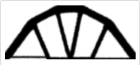
For the optimization process, the prescribed volume fraction of material is set as 0.3, the filter radius is set as 3, the penalization factor 3, and the design domain is discretized with a polygonal mesh with $N=10,000$ finite elements. The non-robust TO of the 2D bridge, performed using PolyTop with MMA optimizer, is shown in Figure 11(b). Furthermore, the first two rows of finite elements on the top of structure are fixed during the optimization process, to ensure that the bridge remains attached to the loading conditions. Allowing the final results to be more realistic. It is observed in Figure 11(b) that the non-robust design leads to a final topology which is similar to the classical case of a 2D bridge under an uniformly distributed load.

For the purpose of numerical computation, the random field $F(\theta,x)$ is discretized by means of $\bm{\xi}=(F_{1})$, a single Gaussian random variable for which low-order statistics are the same as for the random field. The gPC RTO design is obtained using an expansion of order $p_{pc}=5$ (with $1+\nu_{pc}=6$) and a total number of $\nu_{gq}=6$ collocation points for Hermite orthogonal polynomials, and weight factor values $w\in\{0,1,2,3\}$.

The final results are shown in Figure 12, where one can observe that some bars connected at the bottom of the bridge are different from those of the non-robust case in Figure 11(b). Moreover, as the value of $w$ increases, the structure presents a more robust physical form, which represents a consistent result, because the standard deviation of the compliance is being forced to be smaller. The corresponding mean value and standard deviation of the compliance function, for the different values of $w$ employed, are given in Table 4.

As a second analysis, the random load $F(\theta,x)$ is assumed to have the same low-order statistics as before, but an exponentially decaying correlation function

where $l_{corr}$ is a correlation length for the random field. Note that, by this assumption, the loads at any two points $x$, $x^{\prime}$ in the 2D bridge are partially correlated. If the correlation length is increased, a strong correlation is obtained between the points $x$, $x^{\prime}$, so that $l_{corr}=\infty$ implies a perfectly correlated random field — the previous case where the field depends on a single random variable. On the other hand, when $l_{corr}=0$, the random field is completely uncorrelated — many independent random variables are necessary for an accurate computational representation. In order to avoid the two limit cases, $l_{corr}=120$ is chosen.

In terms of computational representation for numerical calculations, the random field $F(\theta,x)$ is discretized with the aid of Karhunen–Loève expansion described in section 2.2. The number of terms in this expansion is chosen in a heuristic way, seeking to satisfy the criterion presented in (16). A good compromise between accuracy and computational efficiency is obtained with $\nu_{kl}=7$. Therefore, the germ is $\bm{\xi}=(F_{1},F_{2},\cdots,F_{\nu_{rv}})$, a set of $\nu_{rv}=7$ independent Gaussian random variables for which low-order statistics are the same as for the random field. Then, for this case we use a total number of $\nu_{gq}=279936$ collocation points.

A comparison between non-robust and gPC RTO design, for $w=1$ and the different types of distributed load considered, are shown in Figure 13. The difference between the three obtained topologies is very clear, and can also be appreciated in Table 5, which shows the low-order statistics of the compliance in all cases analyzed.

References

- Andreasen and Sigmund (2013) Andreasen CS, Sigmund O (2013) Topology optimization of fluid–structure-interaction problems in poroelasticity. Computer Methods in Applied Mechanics and Engineering 258:55–62, DOI https://doi.org/10.1016/j.cma.2013.02.007
- Antonietti et al (2017) Antonietti P, Bruggi M, Scacchi S, Verani M (2017) On the virtual element method for topology optimization on polygonal meshes: A numerical study. Computers & Mathematics with Applications 74(5):1091 – 1109, DOI https://doi.org/10.1016/j.camwa.2017.05.025, URL http://www.sciencedirect.com/science/article/pii/S0898122117303309, sI: SDS2016 – Methods for PDEs
- Asadpoure et al (2011) Asadpoure A, Tootkabonia M, Guest J (2011) Robust topology optimization of structures with uncertainties in stiffness - Application to truss structures. Computers & Structures 89:1031–1041, DOI https://doi.org/10.1016/j.compstruc.2010.11.004
- Atkinson (2009) Atkinson KE (2009) The Numerical Solution of Integral Equations of the Second Kind, reissue edn. Cambridge University Press
- Banichuk and Neittaanmäki (2010) Banichuk N, Neittaanmäki P (2010) Structural Optimization with Uncertainties. Springer Netherlands
- Bellizzi and Sampaio (2012) Bellizzi S, Sampaio R (2012) Smooth decomposition of random fields. Journal of Sound and Vibration 331:3509–3520, DOI https://doi.org/10.1016/j.jsv.2012.03.030
- Bendsøe and Kikuchi (1988) Bendsøe MP, Kikuchi N (1988) Generating optimal topologies in structural design using a homogenization method. Computer Methods in Applied Mechanics and Engineering 71:197–224
- Bendsøe and Sigmund (2004) Bendsøe MP, Sigmund O (2004) Topology Optimization: Theory, Methods, and Applications. Springer-Verlag Berlin Heidelberg
- Betz et al (2014) Betz W, Papaioannou I, Straub D (2014) Numerical methods for the discretization of random fields by means of the Karhunen–Loève expansion. Computer Methods in Applied Mechanics and Engineering 271:109–129, DOI https://doi.org/10.1016/j.cma.2013.12.010
- Beyer and Sendhoff (2007) Beyer HG, Sendhoff B (2007) Robust optimization – A comprehensive survey. Computer Methods in Applied Mechanics and Engineering 196:3190–3218, DOI https://doi.org/10.1016/j.cma.2007.03.003
- Birge and Louveaux (2011) Birge J, Louveaux F (2011) Introduction to Stochastic Programming. Springer-Verlag New York
- Brezis (2010) Brezis H (2010) Functional Analysis, Sobolev Spaces and Partial Differential Equations. Springer-Verlag New York
- Bruggi (2008) Bruggi M (2008) On the solution of the checkerboard problem in mixed-FEM topology optimization. Computers & Structures 86:1819–1829, DOI https://doi.org/10.1016/j.compstruc.2008.04.008
- Chen et al (2010) Chen S, Chen W, Lee S (2010) Level set based robust shape and topology optimization under random field uncertainties. Structural and Multidisciplinary Optimization 41:507–524, DOI https://doi.org/10.1007/s00158-009-0449-2
- Ciarlet (2013) Ciarlet PG (2013) Linear and Nonlinear Functional Analysis with Applications. SIAM
- da Silva and Cardoso (2017) da Silva G, Cardoso E (2017) Stress-based topology optimization of continuum structures under uncertainties. Computer Methods in Applied Mechanics and Engineering 313:647–672, DOI https://doi.org/10.1016/j.cma.2016.09.049
- Dapogny et al (2017) Dapogny C, Faure A, Michailidis G, Allaire G, Couvelas A, Estevez R (2017) Geometric constraints for shape and topology optimization in architectural design. Computational Mechanics 59:933–965, DOI https://doi.org/10.1007/s00466-017-1383-6
- Doltsinis and Kang (2004) Doltsinis I, Kang Z (2004) Robust design of structures using optimization methods. Computer Methods in Applied Mechanics and Engineering 193(23):2221–2237, DOI https://doi.org/10.1016/j.cma.2003.12.055
- Duan et al (2015) Duan XB, Li FF, Qin XQ (2015) Adaptive mesh method for topology optimization of fluid flow. Applied Mathematics Letters 44:40–44, DOI https://doi.org/10.1016/j.aml.2014.12.016
- Dunning and Kim (2013) Dunning PD, Kim HA (2013) Robust topology optimization: Minimization of expected and variance of compliance. AIAA Journal 51:2656–2664, DOI https://doi.org/10.2514/1.J052183
- Eldred (2009) Eldred M (2009) Recent advances in non-intrusive polynomial chaos and stochastic collocation methods for uncertainty analysis and design. In: 50th AIAA/ASME/ASCE/AHS/ASC Structures, Structural Dynamics, and Materials Conference, DOI https://doi.org/10.2514/6.2009-2274
- Ghanem (1999) Ghanem R (1999) Ingredients for a general purpose stochastic finite elements implementation. Computer Methods in Applied Mechanics and Engineering 168:19–34, DOI https://doi.org/10.1016/S0045-7825(98)00106-6
- Ghanem and Red-Horse (2017) Ghanem R, Red-Horse J (2017) Polynomial Chaos: Modeling, Estimation, and Approximation, Springer International Publishing, pp 521–551. DOI https://doi.org/10.1007/978-3-319-12385-1_13
- Ghanem and Spanos (2003) Ghanem RG, Spanos PD (2003) Stochastic Finite Elements: A Spectral Approach, 2nd edn. Dover Publications
- Guest and Igusa (2008) Guest JK, Igusa T (2008) Structural optimization under uncertain loads and nodal locations. Computer Methods in Applied Mechanics and Engineering 198:116–124, DOI https://doi.org/10.1016/j.cma.2008.04.009
- Hoshina et al (2018) Hoshina TYS, Menezes IFM, Pereira A (2018) A simple adaptive mesh refinement scheme for topology optimization using polygonal meshes. Journal of the Brazilian Society of Mechanical Sciences and Engineering 40(7):348, DOI 10.1007/s40430-018-1267-5, URL https://doi.org/10.1007/s40430-018-1267-5
- Jalalpour et al (2013) Jalalpour M, Guest JK, Igusa T (2013) Reliability-based topology optimization of trusses with stochastic stiffness. Structural Safety 43:41–49, DOI https://doi.org/10.1016/j.strusafe.2013.02.003
- Keshavarzzadeh et al (2017) Keshavarzzadeh V, Fernandez F, Tortorelli DA (2017) Topology optimization under uncertainty via non-intrusive polynomial chaos expansion. Computer Methods in Applied Mechanics and Engineering 318:120–147, DOI https://doi.org/10.1016/j.cma.2017.01.019
- Kim et al (2006) Kim NH, Wang H, Queipo NV (2006) Efficient shape optimization under uncertainty using polynomial chaos expansions and local sensitivities. AIAA Journal 44:1112–1116, DOI https://doi.org/10.2514/1.13011
- Kroese et al (2011) Kroese DP, Taimre T, Botev ZI (2011) Handbook of Monte Carlo Methods. Wiley
- Kundu et al (2014) Kundu A, Adhikari S, Friswell M (2014) Stochastic finite elements of discretely parameterized random systems on domains with boundary uncertainty. International Journal for Numerical Methods in Engineering 100(3):183–221
- Kundu et al (2018) Kundu A, Matthies H, Friswell M (2018) Probabilistic optimization of engineering system with prescribed target design in a reduced parameter space. Computer Methods in Applied Mechanics and Engineering 337:281–304
- Luo et al (2017) Luo Y, Niu Y, Li M, Kang Z (2017) A multi-material topology optimization approach for wrinkle-free design of cable-suspended membrane structures. Computational Mechanics 59:967–980, DOI https://doi.org/10.1007/s00466-017-1387-2
- Maître and Knio (2010) Maître OPL, Knio OM (2010) Spectral Methods for Uncertainty Quantification: With Applications to Computational Fluid Dynamics. Springer Netherlands
- Michell M.C.E. (1904) Michell MCE AGM (1904) Lviii. the limits of economy of material in frame-structures. The London, Edinburgh, and Dublin Philosophical Magazine and Journal of Science 8:589–597, DOI https://doi.org/10.1080/14786440409463229
- Nanthakumar et al (2015) Nanthakumar SS, Valizadeh N, Park HS, Rabczuk T (2015) Surface effects on shape and topology optimization of nanostructures. Computational Mechanics 56:97–112, DOI https://doi.org/10.1007/s00466-015-1159-9
- Nguyen-Xuan (2017) Nguyen-Xuan H (2017) A polytree-based adaptive polygonal finite element method for topology optimization. International Journal for Numerical Methods in Engineering 110(10):972–1000, DOI 10.1002/nme.5448, URL https://onlinelibrary.wiley.com/doi/abs/10.1002/nme.5448, https://onlinelibrary.wiley.com/doi/pdf/10.1002/nme.5448
- Park et al (2018) Park J, Sutradhar A, Shah JJ, Paulino GH (2018) Design of complex bone internal structure using topology optimization with perimeter control. Computers in Biology and Medicine pp –, DOI https://doi.org/10.1016/j.compbiomed.2018.01.001
- Pereira et al (2016) Pereira A, Talischi C, Paulino GH, Menezes IFM, Carvalho MS (2016) Fluid flow topology optimization in polytop: stability and computational implementation. Structural and Multidisciplinary Optimization 54:1345–1364, DOI 10.1007/s00158-014-1182-z
- Perrin et al (2013) Perrin G, Soize C, Duhamel D, Funfschilling C (2013) Karhunen–Loève expansion revisited for vector-valued random fields: Scaling, errors and optimal basis. Journal of Computational Physics 242:607–622, DOI https://doi.org/10.1016/j.jcp.2013.02.036
- Pettersson et al (2015) Pettersson MP, Iaccarino G, Nordström J (2015) Polynomial Chaos Methods for Hyperbolic Partial Differential Equations: Numerical Techniques for Fluid Dynamics Problems in the Presence of Uncertainties. Springer International Publishing
- Putek et al (2016) Putek P, Pulch R, Bartel A, ter Maten EJW, Günther M, Gawrylczyk KM (2016) Shape and topology optimization of a permanent-magnet machine under uncertainties. Journal of Mathematics in Industry 6:11, DOI https://doi.org/10.1186/s13362-016-0032-6
- Qizhi et al (2014) Qizhi Q, Kang Z, Wang Y (2014) A topology optimization method for geometrically nonlinear structures with meshless analysis and independent density field interpolation. Computational Mechanics 54:629–644, DOI https://doi.org/10.1007/s00466-014-1011-7
- Richardson et al (2016) Richardson J, Filomeno Coelho R, Adriaenssens S (2016) A unified stochastic framework for robust topology optimization of continuum and truss-like structures. Engineering Optimization 48:334–350, DOI http://dx.doi.org/10.1080/0305215X.2015.1011152
- Romero and Silva (2014) Romero JS, Silva ECN (2014) A topology optimization approach applied to laminar flow machine rotor design. Computer Methods in Applied Mechanics and Engineering 279:268–300, DOI https://doi.org/10.1016/j.cma.2014.06.029
- Rubinstein and Kroese (2016) Rubinstein RY, Kroese DP (2016) Simulation and the Monte Carlo Method, 3rd edn. Wiley
- Shin et al (2011) Shin S, Samanlioglu F, Cho BR, Wiecek MM (2011) Computing trade-offs in robust design: Perspectives of the mean squared error. Computers & Industrial Engineering 60:248 –255, DOI https://doi.org/10.1016/j.cie.2010.11.006
- Sigmund and Petersson (1998) Sigmund O, Petersson J (1998) Numerical instabilities in topology optimization: A survey on procedures dealing with checkerboards, mesh-dependencies and local minima. Structural Optimization 16:68–75, DOI https://doi.org/10.1007/BF01214002
- Soize (2013) Soize C (2013) Stochastic modeling of uncertainties in computational structural dynamics - recent theoretical advances. Journal of Sound and Vibration 332:2379––2395, DOI https://doi.org/10.1016/j.jsv.2011.10.010
- Soize (2015) Soize C (2015) Polynomial chaos expansion of a multimodal random vector. SIAM/ASA Journal on Uncertainty Quantification 3:34–60, DOI https://doi.org/10.1137/140968495
- Soize (2017) Soize C (2017) Uncertainty Quantification: An Accelerated Course with Advanced Applications in Computational Engineering. Springer International Publishing
- Soize and Desceliers (2010) Soize C, Desceliers C (2010) Computational aspects for constructing realizations of polynomial chaos in high dimension. SIAM Journal on Scientific Computing 32:2820–2831, DOI https://doi.org/10.1137/100787830
- Soize and Ghanem (2004) Soize C, Ghanem R (2004) Physical systems with random uncertainties: Chaos representations with arbitrary probability measure. SIAM Journal on Scientific Computing 26:395–410, DOI https://doi.org/10.1137/S1064827503424505
- Soize and Ghanem (2017) Soize C, Ghanem R (2017) Polynomial chaos representation of databases on manifolds. Journal of Computational Physics 335:201–221, DOI https://doi.org/10.1016/j.jcp.2017.01.031
- Spanos and Ghanem (1989) Spanos PD, Ghanem R (1989) Stochastic finite element expansion for random media. Journal of Engineering Mechanics 115:1035–1053, DOI https://doi.org/10.1061/(ASCE)0733-9399(1989)115:5(1035)
- Stefanou (2009) Stefanou G (2009) The stochastic finite element method: Past, present and future. Computer Methods in Applied Mechanics and Engineering 198:1031–1051, DOI https://doi.org/10.1016/j.cma.2008.11.007
- Svanberg (1987) Svanberg K (1987) The method of moving asymptotes—a new method for structural optimization. International Journal for Numerical Methods in Engineering 24:359–373, DOI http://dx.doi.org/10.1002/nme.1620240207
- Talischi et al (2010) Talischi C, Paulino GH, Pereira A, Menezes IFM (2010) Polygonal finite elements for topology optimization: A unifying paradigm. International Journal for Numerical Methods in Engineering 82:671–698, DOI http://dx.doi.org/10.1002/nme.2763
- Talischi et al (2012) Talischi C, Paulino GH, Pereira A, Menezes IFM (2012) PolyTop: a Matlab implementation of a general topology optimization framework using unstructured polygonal finite element meshes. Structural and Multidisciplinary Optimization 45:329–357, DOI https://doi.org/10.1007/s00158-011-0696-x
- Tootkaboni et al (2012) Tootkaboni M, Asadpoure A, Guest JK (2012) Topology optimization of continuum structures under uncertainty – A polynomial chaos approach. Computer Methods in Applied Mechanics and Engineering 201–204:263–275, DOI https://doi.org/10.1016/j.cma.2011.09.009
- Wu et al (2016) Wu J, Gao J, Luo Z, Brown T (2016) Robust topology optimization for structures under interval uncertainty. Advances in Engineering Software 99:36 – 48, DOI https://doi.org/10.1016/j.advengsoft.2016.05.002, URL http://www.sciencedirect.com/science/article/pii/S0965997816300874
- Xia et al (2018) Xia L, Da D, Yvonnet J (2018) Topology optimization for maximizing the fracture resistance of quasi-brittle composites. Computer Methods in Applied Mechanics and Engineering 332:234–254, DOI https://doi.org/10.1016/j.cma.2017.12.021
- Xiu (2010) Xiu D (2010) Numerical Methods for Stochastic Computations: A Spectral Method Approach. Princeton University Press
- Xiu and Karniadakis (2002) Xiu D, Karniadakis GE (2002) The Wiener-Askey Polynomial Chaos for stochastic differential equations. SIAM Journal on Scientific Computing 24:619–644, DOI https://doi.org/10.1137/S1064827501387826
- Zhang and Kang (2017) Zhang W, Kang Z (2017) Robust shape and topology optimization considering geometric uncertainties with stochastic level set perturbation. International Journal for Numerical Methods in Engineering 110:31–56, DOI http://dx.doi.org/10.1002/nme.5344
- Zhang et al (2017) Zhang XS, de Sturler E, Paulino GH (2017) Stochastic sampling for deterministic structural topology optimization with many load cases: Density-based and ground structure approaches. Computer Methods in Applied Mechanics and Engineering 325:463–487, DOI https://doi.org/10.1016/j.cma.2017.06.035
- Zhang et al (2018) Zhang XS, Paulino GH, Ramos AS (2018) Multi-material topology optimization with multiple volume constraints: a general approach applied to ground structures with material nonlinearity. Structural and Multidisciplinary Optimization 57:161–182, DOI https://doi.org/10.1007/s00158-017-1768-3
- Zhao and Wang (2014) Zhao J, Wang C (2014) Robust structural topology optimization under random field loading uncertainty. Structural and Multidisciplinary Optimization 50:517–522, DOI https://doi.org/10.1007/s00158-014-1119-6