∎

Unified Analysis on $L_{1}$ over $L_{2}$ Minimization for signal recovery

Min Tao Affiliation: Department of Mathematics, National Key Laboratory for Novel Software Technology, Nanjing University, Nanjing, 210093, China. E-mail: taom@nju.edu.cn Xiao-Ping Zhang Affiliation: Department of Electrical, Computer and Biomedical Engineering, Ryerson University, Toronto, ON M5B 2K3, Canada.

Received: date / Accepted: date

Abstract

In this paper, we carry out a unified study for $L_{1}$ over $L_{2}$ sparsity promoting models, which are widely used in the regime of coherent dictionaries for recovering sparse nonnegative/arbitrary signals. First, we provide a unified theoretical analysis on the existence of the global solutions of the constrained and the unconstrained $L_{1}/L_{2}$ models. Second, we analyze the sparse property of any local minimizer of these $L_{1}/L_{2}$ models which serves as a certificate to rule out the nonlocal-minimizer stationary solutions. Third, we derive an analytical solution for the proximal operator of the $L_{1}/L_{2}$ with nonnegative constraint. Equipped with this, we apply the alternating direction method of multipliers to the unconstrained model with nonnegative constraint in a particular splitting way, referred to as ADMM ${}_{p}^{+}$ . We establish its global convergence to a d-stationary solution (sharpest stationary) without the Kurdyka-Łojasiewicz assumption. Extensive numerical simulations confirm the superior of ADMM ${}_{p}^{+}$ over the state-of-the-art methods in sparse recovery. In particular, ADMM ${}_{p}^{+}$ reduces computational time by about $95\%\sim 99\%$ while achieving a much higher accuracy than the commonly used scaled gradient projection method for the wavelength misalignment problem.

Keywords:

Sparse recovery fractional programming coherent dictionary d-stationarity

MSC

MSC 90C26 MSC 90C90 49N45

Compressive sensing (CS) is to seek the sparsest solution from a set of undersampled linear measurements. Mathematically, a fundamental problem in CS can be formulated as a constrained model,

\displaystyle\min_{{\mathbf{x}}\in{\cal X}}\|{\mathbf{x}}\|_{0},\;\;s.t.\;\;A{\mathbf{x}}={\mathbf{b}},

(1)

where $A\in\mathbb{R}^{m\times n}(m\ll n)$ is a sensing matrix and the observation of ${\mathbf{b}}\in\mathbb{R}^{n}$ , $\|\cdot\|_{0}$ is the $L_{0}$ norm (the number of nonzero elements). We consider the recovery of nonnegative/arbitrary compressed signal, which corresponds to ${\cal X}=\mathbb{R}^{n}_{+}$ and $\mathbb{R}^{n}$ , respectively. Unfortunately, the optimization (1) is known to be NP-hard BKNa95. One common approach is to relax $L_{0}$ norm to $L_{1}$ norm, leading to basis pursuit model CDS98. Theoretically, the exact recovery by the $L_{1}$ minimization is guaranteed under the restricted isometry property CandesTao05 or null space property AWR09. Although the $L_{1}$ minimization technique has been widely used, it is not able to reconstruct the sparsest solutions when columns of $A$ are highly coherent, such as those applications rising from discretization of continuum image problems (such as medical and radar) when the grid spacing is below the Rayleigh threshold AW12.

As such, various nonconvex regularizers, such as the $L_{p}$ (quasi-)norm ( $0<p<1$ ) CR07, $L_{1}$ - $L_{2}$ YEX14, transform $L_{1}$ NIK00, the ratio of $L_{1}$ over $L_{2}$ norm ( $L_{1}$ / $L_{2}$ ) YEX14 have been developed to enhance the recovery quality. Among these nonconvex regularizations, $L_{1}/L_{2}$ can approximate $L_{0}$ norm very well when the domain is without origin, due to its being scale-invariant and parameter-free as well as $L_{0}$ norm. For one-sparse signal, the $L_{1}/L_{2}$ is the same as the $L_{0}$ norm. The $L_{1}/L_{2}$ arose as sparseness measure Hoy02; HNRS09 and has attracted a considerable attention due to its wide applications, e.g., nonlinear matrix factorization 4541671 and blind deconvolution JSW12; Audrey15.

In this paper, we focus on two commonly-used $L_{1}/L_{2}$ models for signal recovery, i.e., the constrained and the penalized/unconstrained models:

\displaystyle\begin{array}[]{ll}\min_{\mathbf{x}}&\displaystyle{\frac{\|\mathbf{x}\|_{1}}{\|\mathbf{x}\|_{2}}}\\[5.69046pt] s.t.&\mathbf{x}\in\mathcal{H}:=\{{\mathbf{x}}\in{\cal X}\mid A{\mathbf{x}}={\mathbf{b}}\},\end{array}

and

\displaystyle\min_{{\mathbf{x}}\in{\cal X}}F({\mathbf{x}}):=\gamma\frac{\|{\mathbf{x}}\|_{1}}{\|{\mathbf{x}}\|_{2}}+\frac{1}{2}\|A{\mathbf{x}}-\mathbf{b}\|_{2}^{2},

(5)

where $A$ and ${\mathbf{b}}$ are defined identically as in (1). The penalized/unconstrained model (5) can tackle both noisy and noiseless observations while (Unified Analysis on $L_{1}$ over $L_{2}$ Minimization for signal recovery) can only deal with unnoisy data, it is more meaningful to develop efficient and convergent algorithms to solve (5).

First, to recover the signal, we need to solve $L_{1}$ over $L_{2}$ minimization models (Unified Analysis on $L_{1}$ over $L_{2}$ Minimization for signal recovery) or (5). The first question is whether these models are well-defined. Recently, Zeng et al. ZengYuPong20 analyze the existence of global optimal solutions of the constrained model (Unified Analysis on $L_{1}$ over $L_{2}$ Minimization for signal recovery) for the case of ${\cal X}={\mathbb{R}}^{n}$ . However, the nonemptyness of the global solution set of the model of (Unified Analysis on $L_{1}$ over $L_{2}$ Minimization for signal recovery) with ${\cal X}={\mathbb{R}}_{+}^{n}$ and the model (5) with ${\cal X}={{\mathbb{R}}^{n}_{+}}/{\mathbb{R}}^{n}$ (i.e., ${{\mathbb{R}}^{n}_{+}}$ and ${\mathbb{R}}^{n}$ ) have not been studied.

Many early works focus on developing different optimization algorithms for solving $L_{1}/L_{2}$ minimization. To name a few, the scaled gradient projection method (SGPM) ELX13; YEX14 for (5) with ${\cal X}={\mathbb{R}}_{+}^{n}$ , as well as the alternating direction method of multiplier (ADMM) approach RWDL19 for (Unified Analysis on $L_{1}$ over $L_{2}$ Minimization for signal recovery) with ${\cal X}={\mathbb{R}}^{n}$ , accelerated schemes for solving the constrained model (Unified Analysis on $L_{1}$ over $L_{2}$ Minimization for signal recovery) with ${\cal X}={\mathbb{R}}^{n}$ WYYL20, all lack global convergence guarantees. There are two exceptions: Zeng et al. ZengYuPong20 apply moving-balls-approximation based algorithms to solve $L_{1}/L_{2}$ minimization over an inequality constraint for arbitrary signal and prove its local linear convergence under some conditions. Our previous work Tao20 proposes an ADMM-based algorithm for solving (5) with $\mathcal{X}=\mathbb{R}^{n}$ with global convergence guarantee. Although there do exist a few different reformulations for the unconstrained model (5) with $\mathcal{X}=\mathbb{R}_{+}^{n}$ , it turns out that most of these for implementing ADMM result in a violation of convergence guarantee LiPong15; HongLuoRazaviyayn16. It is still unknown how to solve the model (5) with convergence guarantee where $\mathcal{X}=\mathbb{R}^{n}_{+}$ .

In this paper, we carry out a unified theoretical study on (Unified Analysis on $L_{1}$ over $L_{2}$ Minimization for signal recovery) and (5). First, we provide a unified analysis on the existence of global solutions of (Unified Analysis on $L_{1}$ over $L_{2}$ Minimization for signal recovery) and (5). Inspired by ZengYuPong20, we introduce an auxiliary optimization problem and verify that the solution set of (Unified Analysis on $L_{1}$ over $L_{2}$ Minimization for signal recovery) is nonempty if the objective function value of (Unified Analysis on $L_{1}$ over $L_{2}$ Minimization for signal recovery) is strictly less than that of the auxiliary optimization problem. A similar result is also proved for the model (5) while the proof is much more complicated. Then, we illustrate that this sufficient condition can be guaranteed by the $\mu$ -spherical section property of ${\cal N}(A)$ (i.e., the null space of $A$ ) Vavasis. Second, we exploit the sparse property of any local minimizer of (Unified Analysis on $L_{1}$ over $L_{2}$ Minimization for signal recovery) or (5). In particular, we prove that any feasible vector cannot be a local minimizer if the columns of $A$ restricted on the support set are linearly dependent. Third, we design an efficient and convergent algorithm for the penalized model (5) with ${\cal X}={\mathbb{R}}^{n}_{+}$ . To do so, we derive a closed-form solution for one global solution of the proximal operator of $\left(L_{1}/L_{2}\right)^{+}$ (i.e., ${\frac{\|\mathbf{x}\|_{1}}{\|\mathbf{x}\|_{2}}+\iota_{{\mathbb{R}}^{n}_{+}}(\mathbf{x})}$ and $\iota_{{\mathbb{R}}^{n}_{+}}(\mathbf{x})$ is the indicator function of ${\mathbb{R}}^{n}_{+}$ ) and accompanied by a practical solver. Equipped with this, we propose a specific variable-splitting scheme of ADMM for solving (5) with ${\cal X}={\mathbb{R}}^{n}_{+}$ . We referred to it as ADMM ${}_{p}^{+}$ by incorporating the practical proximal solver. Although there already exist many seminal works on convergence analysis for the nonsmooth nonconvex problem, e.g., Attouch13; HongLuoRazaviyayn16; LiPong15, all these convergence results focus on converging to a stationary point which is much weaker than to a d-stationary point DongTao21; PangRazAlv; LSM20. Furthermore, all these approaches achieve global convergence by assuming the introduced merit function with the Kurdyka-Łojasiewicz (KL) property. In contrast, we introduce a novel merit function $\cal T$ (see (41)) instead of the augmented Lagrange function or its variants LiPong15; HongLuoRazaviyayn16 for aiding the global convergence analysis. Then, we establish the global convergence of ADMM ${}_{p}^{+}$ converging to a d-stationary point by proving the merit function with the KL property. We conduct extensive experiments on algorithmic behaviors and various sparse recovery model comparisons, testing on two specific applications. All of these showcase the superior performance of the proposed approach over the state-of-the-art in sparse nonnegative signal recovery. In particular, ADMM ${}_{p}^{+}$ always converges to a more accurate solution (d-stationary) and significantly reduces the computational time in comparison with SGPM and accelerated proximal gradient methods (monotone version with fixed stepsize/line search and its nonmonotone versions). In summary, our contributions are threefold:

(1)

We provide a unified theoretical analysis on the existence of global solutions of the constrained model (Unified Analysis on $L_{1}$ over $L_{2}$ Minimization for signal recovery) and unconstrained model (5).
(2)

We exploit the sparse property of any local minimizer of the constrained model (Unified Analysis on $L_{1}$ over $L_{2}$ Minimization for signal recovery) and unconstrained model (5). This property serves as a certificate to rule out the stationary solution that is not a local minimizer.
(3)

We derive an analytic solution of the proximal operator of $(L_{1}/L_{2})^{+}$ which allows us to design an efficient algorithm for the unconstrained model (5) with ${\cal X}={\mathbb{R}}^{n}_{+}$ , i.e., ADMM ${}_{p}^{+}$ . We establish its global convergence to a d-stationary solution without KL assumption. Extensively numerical simulations further verify the computational efficiency of the ADMM ${}_{p}^{+}$ over the state-of-the-art in sparse recovery.

The rest of this paper proceeds as follows. We describe the notations and definitions in Section 1. In Section 2, we elaborate on the existence of optimal solutions of (Unified Analysis on $L_{1}$ over $L_{2}$ Minimization for signal recovery) and (5). We analyze the sparse property and provide the exact recovery theory for (Unified Analysis on $L_{1}$ over $L_{2}$ Minimization for signal recovery) in Section 3. In Section 4, the proximal operator for $\left(L_{1}/L_{2}\right)^{+}$ is derived. Then, we solve the unconstrained model (5) with ${\cal X}={\mathbb{R}}_{+}^{n}$ via ADMM, where its global convergence is established. Section 5 devotes extensive experiments to showcase the superior performance of the proposed approach in sparse recovery. Conclusions are given in Section 6.

1 Preliminary

We use a bold letter to denote a vector, e.g., ${\mathbf{x}}\in\mathbb{R}^{n}$ , and $x_{i}$ , $\|\mathbf{x}\|_{0}$ and $|{\mathbf{x}}|$ denote the $i$ -th entry of $\mathbf{x}$ , its zero norm of $\mathbf{x}$ and the vector with the absolute value of $\mathbf{x}$ for each entry, respectively. $\|{\mathbf{x}}\|_{2}$ and $\|{\mathbf{x}}\|_{p}$ $(0<p<1)$ denote its 2-norm and $p$ -norm ( $\|{\mathbf{x}}\|_{p}=(\sum_{i=1}^{n}x_{i}^{p})^{1/p}$ ), respectively. The subscript $2$ in $\|\cdot\|_{2}$ is omitted when there is no ambiguity. We use $\mathbb{R}^{n}_{+}$ , $\mathbb{R}^{n}_{-}$ and $\mathbb{R}^{n}_{++}$ to denote the set of nonnegative, nonpositive and positive vectors, respectively. The notation of ${{\bf 1}}$ represents a vector with all entries equal to $1$ . $I_{n}$ is $n\times n$ identity matrix, and $\odot$ presents the componentwise product. We define $[n]:=\{1,2,\ldots,n\}$ . Given an index set $\mathcal{D}\subseteq[n]$ , we use $\sharp(\mathcal{D})$ and $\mathcal{D}^{c}$ to present the cardinality of $\mathcal{D}$ and its complementary set. We specify that ${\cal X}$ is either ${{\mathbb{R}}^{n}_{+}}$ or ${\mathbb{R}}^{n}$ throughout this paper. For a matrix $A\in\mathbb{R}^{m\times n}$ , we denote $A{\cal X}=\left\{{\mathbf{y}}\;\mid\;{\mathbf{y}}=A{\mathbf{x}},\;{\mathbf{x}}\in{\cal X}\right\}$ and refer to the projection onto the closed set of $A\mathcal{X}$ as $\operatorname{Proj}_{(A\mathcal{X})}(\cdot)$ . For a closed set $\mathcal{S}\in\mathbb{R}^{n}$ , we use the notation $\iota_{\cal S}(\mathrm{x})$ to represent the indicator function of the set $\mathcal{S}$ . Given a matrix $A\in\mathbb{R}^{m\times n}$ or a vector $\mathbf{x}\in\mathbb{R}^{n}$ and an index set $\Lambda\subseteq[n],$ we use $A_{\Lambda}$ , ${\mathbf{x}}|_{\Lambda}$ to denote $A[:,i]_{i\in\Lambda}$ and a subvector of $\mathbf{x}$ with entries in $\Lambda,$ respectively. $\mathcal{N}(A)$ denotes the null space of $A$ and $r(A)$ denotes the rank of $A$ . Given a square matrix $A$ , $A\succ{\bf 0}$ means that $A$ is a positive definite matrix. For a vector ${\mathbf{x}}$ , we use the notation of ${\mathbf{x}}\not\leq{\bf 0}$ to represent that not all the entries of ${\mathbf{x}}$ are nonpositive. Given $\epsilon>0$ , we use $\mathcal{B}_{\epsilon}(\hat{\mathbf{x}})$ and $\breve{\mathcal{B}}_{\epsilon}(\hat{\mathbf{x}})$ to denote the open ball of $\{\mathbf{x}\mid\|\mathbf{x}-\hat{\mathbf{x}}\|<\epsilon\}$ and the open ball without the center, respectively. Given two sets of $\mathcal{A}$ and $\mathcal{B},$ we use the notation $\mathcal{A}\backslash\mathcal{B}$ to represent the intersection of $\mathcal{A}$ and the complement of $\mathcal{B}$ . The notation of ${{\mathbb{R}}^{n}_{+}}/{\mathbb{R}}^{n}$ means ${{\mathbb{R}}^{n}_{+}}$ or ${\mathbb{R}}^{n}$ . An extended-real-valued function $f:{\mathbb{R}}^{n}\rightarrow(-\infty,+\infty]$ is said to be proper if its domain ${\text{dom}}f:=\{{\mathbf{x}}\;|\;f(\mathbf{x})<\infty\}$ is nonempty. A proper function $f$ is said to be closed if it is lower semi-continuous. For a proper closed function $f$ and ${\hat{\mathbf{x}}}\in{\text{dom}}f$ , the regular subdifferential ${\hat{\partial}}f({\hat{\mathbf{x}}})$ and the limiting subdifferential $\partial f({\mathbf{x}})$ [24] are defined as

{\hat{\partial}}f({\hat{\mathbf{x}}})=\left\{{\mathbf{v}}\Big|{\mathop{\lim}\limits_{\mathbf{x}\to{\hat{\mathbf{x}}}}}\inf_{{\mathbf{x}}\neq{\hat{\mathbf{x}}}}\frac{f(\mathbf{x})-f(\hat{\mathbf{x}})-\langle{\mathbf{v}},{\mathbf{x}}-{\hat{\mathbf{x}}}\rangle}{\|{\mathbf{x}}-\hat{\mathbf{x}}\|}\geq 0\right\},

\partial f({\hat{\mathbf{x}}}):=\left\{{\mathbf{v}}\Big|\;\exists\;{\mathbf{x}}^{k}\rightarrow{\hat{\mathbf{x}}},\;f({\mathbf{x}}^{k})\rightarrow f(\hat{\mathbf{x}}),{\mathbf{v}}^{k}\in{\hat{\partial}}f({\mathbf{x}}^{k}),{\mathbf{v}}^{k}\rightarrow{\mathbf{v}}\right\},

respectively. Note $\partial\iota_{\mathcal{X}}(\mathbf{x})=\{\mathbf{0}\}$ if $\mathcal{X}=\mathbb{R}^{n},$ and $\partial_{\iota\mathcal{X}}(\mathbf{x})=\left\{{\mathbf{d}}\mid{\mathbf{d}}_{\Lambda}=\mathbf{0},{\mathbf{d}}_{\Lambda^{c}}\leq\mathbf{0},\right.$ $\left.\Lambda={\text{supp}}(\mathbf{x})\right\}$ if $\mathcal{X}=\mathbb{R}_{+}^{n}.$ Throughout the paper, we assume that ${\mathbf{b}}\neq 0$ and ${\cal H}\neq\phi$ . By defining ${\frac{\|{\bf 0}\|_{1}}{\|\bf 0\|_{2}}}=1$ , the objective functions of (Unified Analysis on $L_{1}$ over $L_{2}$ Minimization for signal recovery) and (5) are lower semi-continuous over $\cal X$ . Suppose $f$ be a proper lower semicontinuous function, we define the proximal mapping (RockWets, Definition 1.22): $\prox_{f}(v)=\arg\min_{x}\Big\{f(x)+\frac{1}{2}\|x-v\|^{2}\Big\}.$

For nonconvex and nonsmooth programs, there are various stationary concepts and d-stationary is arguably the sharpest kind among them DongTao21; PangRazAlv; LSM20. A point $\bar{\mathbf{x}}(\neq{\bf 0})\in{\cal X}$ is called a d-stationary point to (5), if it satisfies $F^{\prime}\left({\bar{\mathbf{x}}};{\mathbf{x}}-{\bar{\mathbf{x}}}\right)\geq 0.\quad\forall{\mathbf{x}}\in{\cal X},$ where $F^{\prime}\left({\bar{\mathbf{x}}};{\mathbf{x}}-{\bar{\mathbf{x}}}\right)$ is the directional derivative of $F(\cdot)$ . According to (Clark90, Definition 2.3.4) and (LSM20, Fact 5), $\bar{\mathbf{x}}(\neq{\bf 0})\in{\cal X}$ is a d-stationary point of $(\ref{L1o2uncon})$ if and only if

\displaystyle\left\langle{\mathbf{x}}-{\bar{\mathbf{x}}},\;\gamma\left(\frac{{{\mathbf{1}}}}{\|{\bar{\mathbf{x}}}\|_{2}}-\frac{\|{\bar{\mathbf{x}}}\|_{1}}{\|{\bar{\mathbf{x}}}\|_{2}^{3}}{\bar{\mathbf{x}}}\right)+A^{\top}(A{\bar{\mathbf{x}}}-{\mathbf{b}})\right\rangle\geq 0,\;\;\forall{\mathbf{x}}\!\in{\cal X},\!

(6)

where ${{\mathbf{1}}}\in{\mathbb{R}}^{n}$ by noting that $\frac{\|{\mathbf{x}}\|_{1}}{\|{\mathbf{x}}\|_{2}}+\iota_{{\mathbb{R}}_{+}^{n}}({\mathbf{x}})=\frac{{\bf 1}^{\top}{\mathbf{x}}}{\|\mathbf{x}\|_{2}}+\iota_{{\mathbb{R}}_{+}^{n}}({\mathbf{x}})$ .

Next, we review the concepts of locally sparse set and the uniformity of a vector YEX14 and the KL property BDL07 which is widely used in convergence analysis.

Definition 1

${\mathbf{x}}\in{\cal H}$ is called locally sparse if $\nexists\;{\mathbf{y}}\in{\cal H}\backslash\{{\mathbf{x}}\}$ ( ${\cal H}$ defined in (Unified Analysis on $L_{1}$ over $L_{2}$ Minimization for signal recovery)) such that ${\text{supp}}(\mathbf{y})\subseteq{\text{supp}}(\mathbf{x}).$ Denote by ${\cal H}_{L}=\{\mathbf{x}\in{\cal H}\mid{\mathbf{x}}\;\mbox{is locally sparse}\}$ .

Definition 2

The uniformity of ${\mathbf{x}}$ , $\kappa(\mathbf{x})$ is the ratio between the smallest nonzero absolute entry and the largest one in the sense of absolute value, i.e.

0<\kappa(\mathbf{x}):=\frac{\min_{i\in{\text{supp}}(\mathbf{x})}{|x_{i}|}}{\max_{i\in{\text{supp}}(\mathbf{x})}{|x_{i}|}}\leq 1.

Definition 3

We say a proper closed function $h:\mathbb{R}^{n}\rightarrow(-\infty,+\infty]$ satisfies KL property at a point $\hat{\mathbf{x}}\in{\text{dom}}\partial h$ if there exist a constant $\alpha\in(0,\infty],$ a neighborhood $U$ of ${\mathbf{\hat{x}}}$ , and a continuous concave function $\phi:[0,\nu)\rightarrow[0,\infty)$ with $\phi(0)=0$ such that

(i)

$\phi$ is continuously differentiable on $(0,\nu)$ with $\phi^{\prime}>0$ on $(0,\nu);$
(ii)

for every $\mathrm{x}\in U$ with $h(\hat{\mathbf{x}})<h(\mathbf{x})<h(\hat{\mathbf{x}})+\nu,$ it holds that $\phi^{\prime}(h(\mathbf{x})-h(\hat{\mathbf{x}})){\text{dist}}(\mathbf{0},\partial h({\mathbf{x}}))\geq 1.$

Our analysis on the existence of globally optimal solutions is based on the spherical section property (SSP) Vavasis; ZengYuPong20.

Definition 4

Let $m,\;n$ be two positive integers such that $m<n$ . Let $V$ be an $(n-m)$ -dimensional subspace of $\mathbb{R}^{n}$ and $\mu$ be a positive integer. We say that $V$ has the $\mu$ -spherical section property if $\inf_{\mathbf{v}\in V\backslash\{0\}}\frac{\|\mathbf{v}\|_{1}}{\|\mathbf{v}\|_{2}}\geq\sqrt{\frac{m}{\mu}}.$

If $A\in\mathbb{R}^{m\times n}(m<n)$ is a random matrix with i.i.d. standard Gaussian entries, then its nullspace has the $\mu$ -spherical section property with high probability ZengYuPong20.

Consider the following problem:

\displaystyle\min_{{\mathbf{x}}\in\mathbb{R}^{n}}f({\mathbf{x}})=h({\mathbf{x}})+g({\mathbf{x}}),

(7)

where $h:{\mathbb{R}}^{n}\rightarrow\mathbb{R}$ is $L$ -smooth (possibly, nonconvex) and $g:{\mathbb{R}}^{n}\rightarrow{\mathbb{R}}$ is proper lower semicontinuous function. The forward-backward algorithm generates the iterate as follows:

\displaystyle{\mathbf{x}}^{k+1}\in{\arg\min}_{\mathbf{x}}\prox_{\alpha g}({\mathbf{x}}^{k}-\alpha\nabla h({\mathbf{x}}^{k})),

(8)

where the step size $\alpha\in(0,1/L)$ to guarantee that any accumulation point of the sequence generated above is a stationary point of (7) BLR15; LiPong15.

2 Existence of optimal solutions

We explore the conditions to guarantee the existence of global solutions of (Unified Analysis on $L_{1}$ over $L_{2}$ Minimization for signal recovery) and (5). First, we verify that the solution set of (Unified Analysis on $L_{1}$ over $L_{2}$ Minimization for signal recovery) is nonempty if the optimal value of (Unified Analysis on $L_{1}$ over $L_{2}$ Minimization for signal recovery) is less than that of the auxiliary problem. Second, we prove that the solution set of (5) is nonempty when the objective function value of newly-introduced constrained model is less than the auxiliary problem. Finally, we further show that these sufficient conditions can be guaranteed by the $\mu$ -spherical section property of the null space of the measurement matrix. Our analysis is inspired by ZengYuPong20 and introduce the following auxiliary problem:

\displaystyle\begin{array}[]{ll}f_{dc}^{*}:=&\inf_{{\mathbf{d}}\in{\cal F}_{0}}\displaystyle{\frac{\|\mathbf{d}\|_{1}}{\|\mathbf{d}\|_{2}}}\\[5.69046pt] \mbox{where}&{\cal F}_{0}:=\{{\mathbf{d}}\;\mid\;A\mathbf{d}=\mathbf{0},\;\mathbf{d}\in{\cal X},\;{\mathbf{d}}\neq\mathbf{0}\}.\end{array}

For analysis convenience, we denote the optimal value of (Unified Analysis on $L_{1}$ over $L_{2}$ Minimization for signal recovery) as $f_{pc}^{*}$ and $f_{pc}^{*}<+\infty$ . We recall $\left\{{\mathbf{x}}^{k}\right\}$ is a minimizing sequence of (Unified Analysis on $L_{1}$ over $L_{2}$ Minimization for signal recovery) if ${\mathbf{x}}^{k}\in{\cal H}$ for each $k$ and $\lim_{k\rightarrow\infty}\frac{\left\|{\mathbf{x}}^{k}\right\|_{1}}{\left\|{\mathbf{x}}^{k}\right\|_{2}}=f_{pc}^{*}$ . Therefore we only need to characterize the existence of unbounded minimizing sequence. Before that, we provide a sufficient condition to guarantee the solution set of (2) nonempty.

Lemma 1

Let $f_{dc}^{*}$ be defined in (2). Assume that ${\cal N}(A)\cap{\cal X}\neq\{{\bf 0}\}$ . Then, $f_{dc}^{*}<+\infty$ and the solution set of (2) is nonempty.

Proof

First, the feasible set of (2) is nonempty due to $\mathcal{N}(A)\cap\mathcal{X}\neq\{\bf 0\}$ . The objective function value is lower bounded, i.e., $\frac{\|{\mathbf{d}}\|_{1}}{\|{\mathbf{d}}\|_{2}}\geq 1$ . Suppose that there exists a minimizing sequence $\left\{\tilde{{\mathbf{d}}}^{k}\right\}$ of (2) that is unbounded with $\frac{\left\|\tilde{{\mathbf{d}}}^{k}\right\|_{1}}{\left\|\tilde{{\mathbf{d}}}^{k}\right\|_{2}}\rightarrow f_{dc}^{*}$ as $k\rightarrow+\infty$ . Thus, $f_{dc}^{*}<+\infty$ . Consequently, by defining ${\mathbf{d}}^{k}=\frac{\tilde{{\mathbf{d}}}^{k}}{\|\tilde{{\mathbf{d}}}^{k}\|_{2}}$ , the sequence $\left\{{\mathbf{d}}^{k}\right\}$ is satisfying ${\mathbf{d}}^{k}\in{\cal F}_{0}$ and $\lim_{k\rightarrow+\infty}\frac{\|{\mathbf{d}}^{k}\|_{1}}{\|{\mathbf{d}}^{k}\|_{2}}=f_{dc}^{*}.$ Since the sequence of $\left\{{\mathbf{d}}^{k}\right\}$ is bounded, it has one accumulation point ${\mathbf{d}}^{*}\in{\cal F}_{0}$ . Therefore, the solution value of (2) is attainable by ${\mathbf{d}}^{*}$ .

The following proposition shows that the optimal value of (Unified Analysis on $L_{1}$ over $L_{2}$ Minimization for signal recovery) is upper bounded by that of (2) when the feasible sets of both (Unified Analysis on $L_{1}$ over $L_{2}$ Minimization for signal recovery) and (2) are nonempty.

Proposition 1

Suppose that $\mathcal{N}(A)\cap\mathcal{X}\neq\{\bf 0\}$ . Then, $f_{pc}^{*}\leq f_{dc}^{*}$ .

Proof

Since ${\cal N}(A)\cap{\cal X}\neq\{\bf 0\}$ , it leads to ${\cal F}_{0}\neq\phi$ . For any ${\hat{\mathbf{x}}}\in{\cal H}$ and any ${\hat{\mathbf{d}}}\in{\cal F}_{0}$ , we have ${\hat{\mathbf{x}}}+\tau{\hat{\mathbf{d}}}\in{\cal H}$ where $\tau>0$ . Thus, it leads to $f_{pc}^{*}=\inf_{{\mathbf{x}}\in{\cal H}}\frac{\|\mathbf{x}\|_{1}}{\|\mathbf{x}\|_{2}}\leq\frac{\|{\hat{\mathbf{x}}}+\tau{\hat{\mathbf{d}}}\|_{1}}{\|{\hat{\mathbf{x}}}+\tau{\hat{\mathbf{d}}}\|_{2}}$ . Next, we have that $\lim_{\tau\to+\infty}\frac{\|{\hat{\mathbf{x}}}+\tau{\hat{\mathbf{d}}}\|_{1}}{\|{\hat{\mathbf{x}}}+\tau{\hat{\mathbf{d}}}\|_{2}}=\lim_{\tau\to+\infty}\frac{\|{\hat{\mathbf{x}}}/\tau+{\hat{\mathbf{d}}}\|_{1}}{\|{\hat{\mathbf{x}}}/\tau+{\hat{\mathbf{d}}}\|_{2}}=\frac{\|{\hat{\mathbf{d}}}\|_{1}}{\|{\hat{\mathbf{d}}}\|_{2}}$ . Consequently, for any ${\hat{\mathbf{d}}}\in{\cal F}_{0}$ , it yields that $f_{pc}^{*}\leq\frac{\|{\hat{\mathbf{d}}}\|_{1}}{\|{\hat{\mathbf{d}}}\|_{2}}$ . By taking infimum on both sides of the above inequality with respect to ${\hat{\mathbf{d}}}$ , we have the desired inequality.

Theorem 2.1

Assume that ${\cal N}(A)\cap{\cal X}\neq\{\bf 0\}$ . Consider (Unified Analysis on $L_{1}$ over $L_{2}$ Minimization for signal recovery) and (2). Then, $f_{pc}^{*}=f_{dc}^{*}$ if and only if there exists a minimizing sequence of (Unified Analysis on $L_{1}$ over $L_{2}$ Minimization for signal recovery) that is unbounded.

Proof

For the case of ${\cal X}={\mathbb{R}}^{n},$ it has been proved in (ZengYuPong20, Lemma 3.3) that $f_{pc}^{*}=f_{dc}^{*}$ if and only if there exists a minimizing sequence of (Unified Analysis on $L_{1}$ over $L_{2}$ Minimization for signal recovery) that is unbounded. The proof for the case of ${\cal X}=\mathbb{R}_{+}^{n}$ is similar to the case of ${\cal X}=\mathbb{R}^{n}$ , and thus omitted here.

Corollary 1

Suppose that $\mathcal{N}(A)\cap\mathcal{X}\neq\{\bf 0\}$ . Consider (Unified Analysis on $L_{1}$ over $L_{2}$ Minimization for signal recovery) and (2). If $f_{pc}^{*}<f_{dc}^{*}$ , the solution set of (Unified Analysis on $L_{1}$ over $L_{2}$ Minimization for signal recovery) is nonempty.

Proof

It follows directly by combining Theorem 2.1 and Proposition 1.

Next, we analyze the existence of the global solution of the penalized model (5). In doing so, we introduce a constrained problem parameterized by the vector $\mathbf{c}$ :

\displaystyle\begin{array}[]{ll}\min_{\mathbf{x}}&\displaystyle{\frac{\|\mathbf{x}\|_{1}}{\|\mathbf{x}\|_{2}}}\\[5.69046pt] s.t.&A{\mathbf{x}}={\mathbf{c}},\;{\mathbf{x}}\in{\cal X},\\ \end{array}

and denote the optimal value of (2) as $f_{pc}^{*}(\mathbf{c})$ and $f^{*}_{pc}(\mathbf{c})<+\infty$ for any ${\mathbf{c}}\in A{\cal X}$ .

Theorem 2.2

Suppose that $\mathcal{N}(A)\cap\mathcal{X}\neq\{\bf 0\}$ . Consider (5) and (2). If $f_{pc}^{*}(\mathbf{c})<f_{dc}^{*}$ where ${\mathbf{c}}={\text{Proj}}_{A{\cal X}}(\mathbf{b})$ , the optimal value of (5) can be attainable.

Proof

First, define $r({\mathbf{x}})=\gamma\frac{\|\mathbf{x}\|_{1}}{\|\mathbf{x}\|_{2}}.$ Assume that $\left\{\mathbf{x}^{k}\right\}$ is a minimizing sequence of (5), i.e.,

\displaystyle\lim_{k\rightarrow\infty}F\left({\mathbf{x}}^{k}\right)=F^{*}.

(15)

If the sequence $\left\{{\mathbf{x}}^{k}\right\}$ is bounded, then it has a subsequence $\left\{{\mathbf{x}}^{k_{j}}\right\}$ converging to some ${\mathbf{x}}^{*}$ . Hence, ${\mathbf{x}}^{*}$ is an optimal solution of (5). Otherwise, the sequence $\left\{{\mathbf{x}}^{k}\right\}$ is unbounded, i.e., $\|\mathbf{x}^{k}\|\to\infty$ as $k\to\infty$ . Since the sequence of $\{r(\mathbf{x}^{k})\}$ is bounded below and $F^{*}$ is finite, it leads to the sequence of $\{\frac{1}{2}\|A{\mathbf{x}}^{k}-{\mathbf{b}}\|^{2}_{2}\}$ is bounded above. It implies that the subsequence of $\{A{\mathbf{x}}^{k}\}$ is bounded. Since $\{A{\mathbf{x}}^{k}\}$ is bounded, it has a sequence that converges to ${\mathbf{y}}^{*}$ . Without loss of generality, we assume that $A{\mathbf{x}}^{k}\rightarrow{\mathbf{y}}^{*}$ . Let ${\cal I}=\{j:\;\{x_{j}^{k}\}\;\mbox{is bounded}\}$ . Then, it follows that $\{A_{{\cal I}}{\mathbf{x}}_{\cal I}^{k}\}$ is bounded. This together with boundedness of $\{A{\mathbf{x}}^{k}\}$ implies that $\{A_{{\cal I}^{c}}{\mathbf{x}}_{{\cal I}^{c}}^{k}\}$ is also bounded. Next, for each $k$ , we consider the following linear system, $A_{{\cal I}^{c}}{\mathbf{y}}^{k}=A_{{\cal I}^{c}}{\mathbf{x}}_{{\cal I}^{c}}^{k},\;{\mathbf{y}}^{k}\in{\cal Y},$ where ${\cal Y}:={\mathbb{R}}^{\sharp({\cal I}^{c})}$ if ${\cal X}={\mathbb{R}}^{n}$ and ${\cal Y}:={\mathbb{R}}_{+}^{\sharp({\cal I}^{c})}$ if ${\cal X}={\mathbb{R}}_{+}^{n}$ . Obviously, the solution set of the above linear system is nonempty due to at least one solution $\mathbf{y}^{k}={\mathbf{x}}^{k}_{{\cal I}^{c}}$ for each $k$ . Using Hoffman’s Error Bound Hoffman1952OnAS, there exist a vector $\mathbf{y}^{k}$ satisfying $A_{{\cal I}^{c}}{\mathbf{y}}^{k}=A_{{\cal I}^{c}}{\mathbf{x}}_{{\cal I}^{c}}^{k}$ and a constant $\zeta>0$ depending only on $A_{{\cal I}^{c}}$ such that

\displaystyle\|\mathbf{y}^{k}\|\leq\zeta\|A_{{\cal I}^{c}}{\mathbf{x}}_{{\cal I}^{c}}^{k}\|.

By setting ${\hat{\mathbf{x}}}^{k}=({\mathbf{x}}_{{\cal I}}^{k},{\mathbf{y}}^{k})$ , it leads to $A{\hat{\mathbf{x}}^{k}}=A{\mathbf{x}}^{k}$ and ${\hat{\mathbf{x}}}^{k}\rightarrow{\mathbf{x}}^{*}$ for convenience due to its boundedness of $\{{\hat{\mathbf{x}}}^{k}\}$ . Obviously, ${\mathbf{y}}^{*}=A{\mathbf{x}}^{*}$ thanks to $A{\hat{\mathbf{x}}}^{k_{j}}=A{\mathbf{x}}^{k_{j}}$ . In the following, we divide into two cases to verify.
Case 1. If there exists two subsequences $\{{\mathbf{x}}^{k_{j}}\}$ and $\{{\hat{\mathbf{x}}^{k_{j}}}\}$ such that

\displaystyle\frac{\|{\mathbf{x}}^{k_{j}}\|_{1}}{\|{\mathbf{x}}^{k_{j}}\|_{2}}\geq\frac{\|{\hat{\mathbf{x}}}^{k_{j}}\|_{1}}{\|{\hat{\mathbf{x}}}^{k_{j}}\|_{2}},\;\;\forall\;j.

(16)

Since $A{\hat{\mathbf{x}}}^{k_{j}}=A{\mathbf{x}}^{k_{j}}$ , we have that $F({\mathbf{x}}^{k_{j}})\geq F({\hat{\mathbf{x}}}^{k_{j}}).$ By using ${\hat{\mathbf{x}}}^{k_{j}}\rightarrow{\mathbf{x}}^{*}$ and $F$ lower semi-continuous, it yields that $\mathop{\underline{\lim}}\limits_{j\to\infty}F({\hat{\mathbf{x}}}^{k_{j}})\geq F({\mathbf{x}}^{*}).$ On the other hand,

\displaystyle F^{*}=\mathop{{\lim}}\limits_{k\to\infty}F({{\mathbf{x}}}^{k})=\mathop{{\lim}}\limits_{j\to\infty}F({{\mathbf{x}}}^{k_{j}})\geq\mathop{\underline{\lim}}\limits_{j\to\infty}F({\hat{\mathbf{x}}}^{k_{j}})\geq F({\mathbf{x}}^{*}).

Invoking the definition of $F^{*}$ , it leads to $F({\mathbf{x}}^{*})=F^{*}$ and ${\mathbf{x}}^{*}$ is an optimal solution.
Case 2. If there does not exist such two sequences $\{{\mathbf{x}}^{k_{j}}\}$ and $\{{\hat{\mathbf{x}}}^{k_{j}}\}$ satisfying (16), it implies there exists an index $K$ such that $\frac{\|{\mathbf{x}}^{k}\|_{1}}{\|{\mathbf{x}}^{k}\|_{2}}<\frac{\|{\hat{\mathbf{x}}}^{k}\|_{1}}{\|{\hat{\mathbf{x}}}^{k}\|_{2}},\;\;\forall\;k\geq K.$ Next, we further divide into two cases to verify.

(a)

Suppose that ${\mathbf{y}}^{*}\in{\text{Proj}}_{(A{\cal X})}({\mathbf{b}})$ . Then, the solution set of (2) with ${\mathbf{c}}={\mathbf{y}}^{*}$ is nonempty due to $f_{pc}^{*}({\mathbf{y}}^{*})<f_{dc}^{*}$ . We assume that ${\hat{\mathbf{x}}}$ is an optimal solution of (2) with ${\mathbf{c}}={\mathbf{y}}^{*}$ . Since (15) and $A{\mathbf{x}}^{k}\to{\mathbf{y}}^{*}$ , then

\displaystyle\lim_{k\to\infty}\frac{\|{\mathbf{x}}^{k}\|_{1}}{\|{\mathbf{x}}^{k}\|_{2}}=(F^{*}-\frac{1}{2}\|{\mathbf{y}}^{*}-{\mathbf{b}}\|_{2}^{2})<+\infty.

Next, we verify that

\displaystyle\lim_{k\to\infty}\frac{\|{\mathbf{x}}^{k}\|_{1}}{\|{\mathbf{x}}^{k}\|_{2}}\leq\frac{\|{\hat{\mathbf{x}}}\|_{1}}{\|{\hat{\mathbf{x}}}\|_{2}}=f_{pc}^{*}({\mathbf{y}}^{*}).

(17)

Suppose not, i.e., $\lim_{k\to\infty}\frac{\|{\mathbf{x}}^{k}\|_{1}}{\|{\mathbf{x}}^{k}\|_{2}}>\frac{\|{\hat{\mathbf{x}}}\|_{1}}{\|{\hat{\mathbf{x}}}\|_{2}}$ , it implies that $F({\hat{\mathbf{x}}})<F^{*}$ since $A{\hat{\mathbf{x}}}=A{\mathbf{x}}^{*}={\mathbf{y}}^{*}$ . It contradicts the definition of $F^{*}$ . Thus, (17) holds. We define ${\tilde{\mathbf{x}}^{k}}:=\frac{{\mathbf{x}}^{k}}{\|\mathbf{x}^{k}\|_{2}}$ . Taking $k\to\infty$ , $A{\mathbf{x}}^{k}\rightarrow{\mathbf{y}}^{*}\;\Rightarrow\;A{\tilde{\mathbf{x}}}^{k}\rightarrow{\bf 0},$ since $\|{\mathbf{x}}^{k}\|_{2}\to\infty$ . Since ${\tilde{\mathbf{x}}}^{k}$ is bounded, it has a subsequence ${\tilde{\mathbf{x}}}^{k_{j}}\rightarrow{\bar{\mathbf{x}}}$ where ${\bar{\mathbf{x}}}$ satisfies ${\bar{\mathbf{x}}}\in{\cal F}_{0}$ .

\displaystyle\mathop{\lim}\limits_{k\to\infty}\frac{\|{\mathbf{x}}^{k}\|_{1}}{\|{\mathbf{x}}^{k}\|_{2}}=\frac{\|{\bar{\mathbf{x}}}\|_{1}}{\|{\bar{\mathbf{x}}}\|_{2}}\geq f_{dc}^{*}>f_{pc}^{*}({\mathbf{y}}^{*}),

(18)

where the first inequality is due to ${\bar{\mathbf{x}}}\in{\cal F}_{0}$ and the last inequality follows from ${\mathbf{y}}^{*}\in{\text{Proj}}_{A{\cal X}}(\mathbf{b})$ . Note that the above inequality contradicts (17). Hence, this case cannot happen.

(b)

Suppose that ${\mathbf{y}}^{*}\not\in{\text{Proj}}_{A{\cal X}}(\mathbf{b})$ . Then, we choose one vector ${\hat{\mathbf{y}}}\in{\text{Proj}}_{A{\cal X}}({\mathbf{b}})$ . Consider the constrained problem (2) with ${\mathbf{c}}:={\hat{\mathbf{y}}}$ . Since $f^{*}_{pc}({\hat{\mathbf{y}}})<f_{dc}^{*}$ , the solution set of (2) with ${\mathbf{c}}:={\hat{\mathbf{y}}}$ is nonempty due to Corollary 1. We assume that $\breve{{\mathbf{x}}}$ is an optimal solution of (2) with ${\mathbf{c}}:={\hat{\mathbf{y}}}$ . Similar to case (a), one can derive a version of (18) as follows

\displaystyle\mathop{\lim}\limits_{k\to\infty}\gamma\frac{\|\mathbf{x}^{k}\|_{1}}{\|\mathbf{x}^{k}\|_{2}}=\gamma\frac{\|{\bar{\mathbf{x}}}\|_{1}}{\|{\bar{\mathbf{x}}}\|_{2}}\geq\gamma f_{dc}^{*},

(19)

where the definition of ${\bar{\mathbf{x}}}$ is the same as Case (a). By noting ${\hat{\mathbf{y}}}\in{\text{Proj}}_{A{\cal X}}(\mathbf{b})$ and ${\mathbf{y}}^{*}\in A{\cal X}$ since $A{\mathbf{x}}^{k}\in A{\cal X}$ and $A{\mathbf{x}}^{k}\to{\mathbf{y}}^{*}$ , it leads to $\frac{1}{2}\|{\hat{\mathbf{y}}}-{\mathbf{b}}\|^{2}\leq\frac{1}{2}\|{\mathbf{y}}^{*}-{\mathbf{b}}\|^{2}.$ Thus, $\frac{1}{2}\|A\breve{\mathbf{x}}-{\mathbf{b}}\|^{2}\leq\frac{1}{2}\|{\mathbf{y}}^{*}-{\mathbf{b}}\|^{2}$ . By noting $r(\breve{\mathbf{x}})=\gamma f_{pc}^{*}({\hat{\mathbf{y}}})<\gamma f_{dc}^{*}$ , and combining with the above inequality, it yields that

\displaystyle F(\breve{\mathbf{x}})<\gamma f_{dc}^{*}+\frac{1}{2}\|{\mathbf{y}}^{*}-{\mathbf{b}}\|^{2}.

(20)

On the other hand, combining (19) with the fact of $A{\mathbf{x}}^{k}\rightarrow{\mathbf{y}}^{*}$ , we have

\displaystyle\gamma f_{dc}^{*}+\frac{1}{2}\|{\mathbf{y}}^{*}-{\mathbf{b}}\|^{2}\leq\mathop{\lim}\limits_{k\to\infty}\left(\gamma\frac{\|\mathbf{x}^{k}\|_{1}}{\|\mathbf{x}^{k}\|_{2}}+\frac{1}{2}\|A{\mathbf{x}}^{k}-{\mathbf{b}}\|_{2}^{2}\right)=F^{*}.

In view of (20) and the above inequality, it leads to $F(\breve{\mathbf{x}})<F^{*}$ which contradicts the definition of $F^{*}$ .

Thus, the sequence $\{{\mathbf{x}}^{k}\}$ is bounded, and thus it has an accumulation point ${\mathbf{x}}^{*}$ which is an optimal solution of (5).

Next, we present the theorem on the existence of global solutions of (Unified Analysis on $L_{1}$ over $L_{2}$ Minimization for signal recovery) and (5). The proof follows the line of arguments as in (ZengYuPong20, Theorem 3.4), thus omitted here.

Theorem 2.3

Consider (Unified Analysis on $L_{1}$ over $L_{2}$ Minimization for signal recovery) and (5). Suppose that ${\cal N}(A)$ has the $\mu$ -spherical section property for some $\mu>0$ . Then, the following assertions hold:

(i)

If there exists ${\hat{\mathbf{x}}}\in{\mathbb{R}}^{n}$ such that $\|\hat{\mathbf{x}}\|_{0}<m/\mu$ , ${\hat{\mathbf{x}}}\in{\cal X}$ and $A{\hat{\mathbf{x}}}={\mathbf{b}}$ , then the set of optimal solution of (Unified Analysis on $L_{1}$ over $L_{2}$ Minimization for signal recovery) is nonempty.
(ii)

If there exists ${\hat{\mathbf{x}}}\in\mathbb{R}^{n}$ such that $\|\hat{\mathbf{x}}\|_{0}<m/\mu$ , ${\hat{\mathbf{x}}}\in{\cal X}$ , and $A{\hat{\mathbf{x}}}={\mathbf{c}}$ where ${\mathbf{c}}={\text{Proj}}_{A{\cal X}}(\mathbf{b})$ , then the set of optimal solutions of (5) is nonempty.

Next, we consider how to guarantee ${\bf 0}$ not being a globally optimal solutions for (Unified Analysis on $L_{1}$ over $L_{2}$ Minimization for signal recovery) and (5). In view of ${\mathbf{b}}\neq{\bf 0}$ , ${\bf 0}$ cannot be a globally optimal solution of the constrained model (Unified Analysis on $L_{1}$ over $L_{2}$ Minimization for signal recovery). In Theorem 2.4, we provide sufficient conditions to guarantee that ${\bf 0}$ cannot be a globally optimal solution of (5).

Theorem 2.4

Suppose that one of the following assumptions holds:

(i)

${\mathbf{b}}\in A{\cal X}$ and $0<\gamma<\frac{\|{\mathbf{b}}\|_{2}^{2}}{2(\sqrt{n}-1)}$ ;
(ii)

There exists a vector ${\hat{\mathbf{x}}}\in{\cal X}$ such that $\|A{\hat{\mathbf{x}}}-{\mathbf{b}}\|_{2}\leq\varepsilon\;(\varepsilon\ll\|{\mathbf{b}}\|_{2})$ and $0<\gamma<\frac{\|{\mathbf{b}}\|_{2}^{2}-\varepsilon^{2}}{2(\sqrt{n}-1)}$ .

Then, the optimal solution of (5) cannot be ${\bf 0}$ .

Proof

(i) We use contradiction to show it. Suppose that ${\bf 0}$ is a global solution of (5). Since ${\mathbf{b}}\in A{\cal X}$ , we choose a vector ${\tilde{\mathbf{x}}}\in{\cal X}$ such that $A{\tilde{\mathbf{x}}}={\mathbf{b}}$ . Then, it leads to $\gamma\sqrt{n}<\gamma+\frac{1}{2}\|\mathbf{b}\|^{2}$ which implies that $F({\tilde{\mathbf{x}}})<F({\bf 0})$ . It contradicts to ${\bf 0}$ being a global solution of (5). (ii) The proof is similar to (i), thus omitted here.

Remark 1

The assumptions of (i) and (ii) in Theorem 2.4 correspond to the cases of noiseless and noisy observations, respectively.

3 Sparse property

We demonstrate the sparsity of the local minimizers of (Unified Analysis on $L_{1}$ over $L_{2}$ Minimization for signal recovery) and (5) in the sense that minimizing $L_{1}/L_{2}$ or $(L_{1}/L_{2})^{+}$ only extract linearly independent columns from the sensing matrix $A$ . With this, we provide a much more easily checkable exact recovery condition than (YEX14, Theorem III.2) for the constrained model both for arbitrary and nonnegative signals.

Theorem 3.1

Let ${\mathbf{x}}^{*}$ $({\mathbf{x}}^{*}\neq{\bf 0})$ be a local minimizer of the constrained problem (Unified Analysis on $L_{1}$ over $L_{2}$ Minimization for signal recovery) and $\Lambda^{*}={\text{supp}}(\mathbf{x}^{*})$ . Then, $(A_{{\Lambda}^{*}})^{\top}(A_{\Lambda^{*}})\succ{\bf 0}.$

Proof

We divide into two cases to verify.
Case 1. ${\cal X}={\mathbb{R}}^{n}$ . Let ${\mathbf{x}}^{*}$ be a local minimizer of the constrained model (Unified Analysis on $L_{1}$ over $L_{2}$ Minimization for signal recovery). We use contradiction. Suppose the columns of $A_{\Lambda^{*}}$ are linearly dependent; then there exists ${\bf v}\neq{\bf 0}$ and ${\mathbf{v}}\in{\cal N}(A)$ such that ${\text{supp}}(\mathbf{v})\subseteq\Lambda^{*}$ . For any fixed neighborhood ${\cal B}_{r}(\mathbf{x}^{*})$ of ${\mathbf{x}}^{*}$ , we scale $\mathbf{v}$ so that $\|\mathbf{v}\|_{2}<\min\{\mathop{\min}\limits_{i\in{{\Lambda}^{*}}}|x_{i}^{*}|,\;r\}.$ Consider two feasible vectors in ${\cal B}_{r}({\mathbf{x}}^{*})$ , ${\hat{\mathbf{x}}}={\mathbf{x}}^{*}+{\mathbf{v}}$ and $\check{\mathbf{x}}={\mathbf{x}}^{*}-{\mathbf{v}}$ . Since ${\text{supp}}(\mathbf{v})\subseteq\Lambda^{*}$ , we have ${\text{supp}}({\hat{\mathbf{x}}})\subseteq{\Lambda}^{*}$ and ${\text{supp}}(\check{\mathbf{x}})\subseteq{\Lambda}^{*}$ . Since for any $i\in{\Lambda}^{*}$ , $|x_{i}^{*}|\pm{\text{sign}}(x_{i}^{*})v_{i}\geq\mathop{\min}\limits_{i\in{\Lambda}^{*}}|x_{i}^{*}|-\|\mathbf{v}\|_{2}>0,\;\forall\;i\in{\Lambda}^{*}$ . Thus, $({\mathbf{x}}^{*}\pm{\mathbf{v}})_{i}={\text{sign}}(x_{i}^{*})(|x_{i}^{*}|\pm{\text{sign}}(x_{i}^{*})v_{i})$ for any $i\in\Lambda^{*}.$ It implies that ${\mathbf{x}}^{*}$ , ${\hat{\mathbf{x}}}$ and $\check{\mathbf{x}}$ are located in the same octant. Consequently, $\|\mathbf{x}^{*}\|_{1}=\frac{1}{2}\left(\|{\hat{\mathbf{x}}}\|_{1}+\|\check{\mathbf{x}}\|_{1}\right),\;\|\mathbf{x}^{*}\|_{2}<\frac{1}{2}\left(\|{\hat{\mathbf{x}}}\|_{2}+\|\check{\mathbf{x}}\|_{2}\right)$ . Suppose not. Then, there exists a positive scalar $\kappa$ ( $\neq 1$ ) such that $\check{\mathbf{x}}=\kappa{\hat{\mathbf{x}}}$ which contradicts the facts of $A{\hat{\mathbf{x}}}={\mathbf{b}}$ and $A{\mathbf{\check{x}}}={\mathbf{b}}$ . Finally, it yields that $\frac{\|\mathbf{x}^{*}\|_{1}}{\|\mathbf{x}^{*}\|_{2}}>\min\left\{\frac{\|{\hat{\mathbf{x}}}\|_{1}}{\|{\hat{\mathbf{x}}}\|_{2}},\frac{\|{\check{\mathbf{x}}}\|_{1}}{\|{\check{\mathbf{x}}}\|_{2}}\right\},$ which contradicts the fact that ${\mathbf{x}}^{*}$ is a local minimizer.
Case 2. ${\cal X}={\mathbb{R}}_{+}^{n}$ . The proof is similar to Case 1, thus omitted here.

Next, we show that the conclusion of Theorem 3.1 also holds for the unconstrained model.

Theorem 3.2

Let ${\mathbf{x}}^{*}$ be a local minimizer of the unconstrained problem (5) and ${\Lambda^{*}}={\text{supp}}({\mathbf{x}}^{*})$ . Then, $(A_{\Lambda^{*}})^{\top}(A_{\Lambda^{*}})\succ{\bf 0}.$

Proof

First, we show that ${\mathbf{x}}^{*}$ is also a local minimizer of the constrained problem (Unified Analysis on $L_{1}$ over $L_{2}$ Minimization for signal recovery) where ${\mathbf{b}}:=A{\mathbf{x}}^{*}$ . Suppose not. Then, for any $r>0$ , there exists ${\mathbf{x}}_{r}\in{\cal B}_{r}(\mathbf{x}^{*})\cap{\cal X}$ such that $A{\mathbf{x}}_{r}=A{\mathbf{x}}^{*}$ and $\frac{\|{\mathbf{x}}_{r}\|_{1}}{\|{\mathbf{x}}_{r}\|_{2}}<\frac{\|{\mathbf{x}}^{*}\|_{1}}{\|{\mathbf{x}}^{*}\|_{2}}.$ It further implies that $F({\mathbf{x}}_{r})<F({\mathbf{x}}^{*})$ where $F$ is defined in (5), which contradicts that ${\mathbf{x}}^{*}$ is a local minimizer of (5). Therefore, ${\mathbf{x}}^{*}$ is a local minimizer of (Unified Analysis on $L_{1}$ over $L_{2}$ Minimization for signal recovery) where ${\mathbf{b}}:=A{\mathbf{x}}^{*}$ . By invoking Theorem 3.1, the conclusion follows directly.

Remark 2

From Theorems 3.1 and 3.2, we see that if a computed solution ${\mathbf{x}}$ from the model (Unified Analysis on $L_{1}$ over $L_{2}$ Minimization for signal recovery) or (5) fails to extract linearly independent columns from the sensing matrix $A$ . Then, ${\mathbf{x}}$ cannot be a local minimizer.

The next lemma presents a sufficient and necessary condition for characterizing ${\mathbf{x}}\in{\cal H}_{L}$ which turns out to be checkable.

Lemma 2

${\mathbf{x}}\in{\cal H}_{L}$ if and only if $A^{\top}_{\Lambda}A_{\Lambda}\succ{\bf 0}\;\mbox{where}\;\Lambda={\text{supp}}(\mathbf{x})$ .

Proof

We use contradiction to show the direction of “only if”. Let $\alpha=\sharp(\Lambda)$ . Suppose not. It implies that there exists a vector ${\mathbf{v}}\in{\mathbb{R}}^{\alpha}\;({\mathbf{v}}\neq{\bf 0})$ such that ${\mathbf{v}}\in{\cal N}(A_{\Lambda})$ . Thus, there exists a vector ${\tilde{\mathbf{v}}}\in{\mathbb{R}}^{n}$ such that $({\tilde{\mathbf{v}}})|_{\Lambda}={\mathbf{v}}$ and $({\tilde{\mathbf{v}}})|_{\Lambda^{c}}={\bf 0}$ . We define an index set: $\Lambda_{{\tilde{\mathbf{v}}}}:={\text{supp}}({\tilde{\mathbf{v}}})$ . Note that ${\text{supp}}({\tilde{\mathbf{v}}})\subseteq\Lambda$ . Let $\zeta:=\min_{i\in\Lambda_{{\tilde{\mathbf{v}}}}}|\frac{x_{i}}{{\tilde{v}}_{i}}|>0$ and ${\tilde{i}}\in\arg\min_{i\in\Lambda_{{\tilde{\mathbf{v}}}}}|\frac{x_{i}}{{\tilde{v}}_{i}}|$ . Next, we define the vector: ${\tilde{\mathbf{x}}}={\mathbf{x}}-{\text{sign}}(x_{\tilde{i}}{\tilde{v}}_{\tilde{i}})\zeta{\tilde{\mathbf{v}}}.$ Then, ${\tilde{\mathbf{x}}}\in{\cal H}$ , and it is much sparser than $\mathbf{x}$ and ${\text{supp}}({\tilde{\mathbf{x}}})\subseteq{\text{supp}}(\mathbf{x})$ which contradicts ${\mathbf{x}}\in{\cal H}_{L}$ . Second, for the direction of “if”, we also use contradiction. Suppose there exists a feasible solution $\mathbf{y}(\neq{\mathbf{x}})$ such that ${{\text{supp}}(\mathbf{y})}\subseteq{{\text{supp}}}({\mathbf{x}})$ , and $A{\mathbf{y}}={\mathbf{b}}$ , ${\mathbf{y}}\in{\cal X}$ . Then, define ${\mathbf{v}}:={\mathbf{y}}-{\mathbf{x}}(\neq{\bf 0})\in{\cal N}(A_{\Lambda})$ which contradicts $(A_{\Lambda})^{\top}(A_{\Lambda})\succ{\bf 0}$ .

Combining Theorems 3.1, 3.2 and Lemma 2, we conclude the following corollary.

Corollary 2

We have these facts hold:

(i)

Suppose that $rank(A)=m$ and ${\mathbf{x}}^{*}$ is a local minimizer of (Unified Analysis on $L_{1}$ over $L_{2}$ Minimization for signal recovery) and (5), the sparsity of ${\mathbf{x}}^{*}$ is at most $m$ .
(ii)

The model (Unified Analysis on $L_{1}$ over $L_{2}$ Minimization for signal recovery) has a finite number of local minimizers.
(iii)

If ${\mathbf{x}}^{*}$ is a local minimizer of (Unified Analysis on $L_{1}$ over $L_{2}$ Minimization for signal recovery), then ${\mathbf{x}}^{*}\in{\cal H}_{L}$ where ${\cal H}_{L}$ is defined in Definition 1.

Proof

The proof for (i) and (ii) are elementary, thus omitted. (iii) It follows from Theorems 3.1, 3.2 and Lemma 2 directly.

Equipped with Lemma 2, we provide an exact recovery condition of the constrained model (Unified Analysis on $L_{1}$ over $L_{2}$ Minimization for signal recovery) which extends (YEX14, Theorem III.2) to nonnegative/arbitrary signal and turns out to be much easier to check. The proof is analogous to (YEX14, Theorem III.2), thus omitted.

Theorem 3.3

If ${\mathbf{x}}_{0}$ uniquely solves (1) and $\|{\mathbf{x}}_{0}\|_{0}=s$ and if

\displaystyle\kappa(\mathbf{x})>\frac{(\sqrt{\|\mathbf{x}\|_{0}}-\sqrt{\|\mathbf{x}\|_{0}-s})^{2}}{s},\;\;\forall\;{\mathbf{x}}\in{\tilde{\cal F}}\backslash\{{\mathbf{x}}_{0}\},

(21)

${\tilde{\cal F}}:=\{{\mathbf{x}}\in{\cal H}\;|\;\Lambda={\text{supp}}(\mathbf{x}),\;A_{\Lambda}^{\top}A_{\Lambda}\succ{\bf 0}\},$ where ${\cal H}$ is defined in (Unified Analysis on $L_{1}$ over $L_{2}$ Minimization for signal recovery). Then, ${\mathbf{x}}_{0}$ also uniquely solves (Unified Analysis on $L_{1}$ over $L_{2}$ Minimization for signal recovery).

4 Computational approach

We focus on solving (5) with ${\cal X}=\mathbb{R}_{+}^{n}$ . Inspired by Tao20, we derive the closed-form solution of the proximal operator of $(L_{1}/L_{2})^{+}$ , and accompanied by a practical solver for finding one global solution.

4.1 Proximal operator

Define a proximal operator of $\left(L_{1}/L_{2}\right)^{+}(:=\frac{\|\mathbf{x}\|_{1}}{\|\mathbf{x}\|_{2}}+\iota_{{\mathbb{R}}^{n}_{+}}(\mathbf{x}))$ with a parameter $\rho>0$ as

\displaystyle\prox_{[({L}_{1}/{L}_{2})^{+}/\rho]}(\mathbf{q}):={\arg\min}_{\mathbf{x}\in{\mathbb{R}}_{+}^{n}}\Big(\frac{\|\mathbf{x}\|_{1}}{\|\mathbf{x}\|_{2}}+\frac{\rho}{2}\|\mathbf{x}-\mathbf{q}\|_{2}^{2}\Big).

(22)

It follows from (RockWets, Definition 1.23) and (RockWets, Theorem 1.25), the solution set of (22) is nonempty. Obviously, if ${\mathbf{q}}\in{\mathbb{R}}^{n}_{-}$ , the solution of (22) is ${\bf 0}$ . Next, Example 1 shows that the optimal solution of (22) may not be unique.

Example 1. Let $n=2$ and $q_{1}=q_{2}=\sqrt{2(\sqrt{2}-1)}$ . Consider an objective function

\displaystyle\min_{{\mathbf{x}}\in{\mathbb{R}}^{n}_{+}}\frac{\left|x_{1}\right|+\left|x_{2}\right|}{\sqrt{x_{1}^{2}+x_{2}^{2}}}+\frac{1}{2}\left(x_{1}-q_{1}\right)^{2}+\frac{1}{2}\left(x_{2}-q_{2}\right)^{2}.

Indeed, it has three globally optimal solutions:

\displaystyle{\mathbf{x}}_{1}=(\sqrt{2(\sqrt{2}-1)},0)^{\top},\;{\mathbf{x}}_{2}=(0,\sqrt{2(\sqrt{2}-1)})^{\top}\;\;\mbox{and}\;\;{\mathbf{x}}_{3}=\left(\sqrt{2(\sqrt{2}-1)},\sqrt{2(\sqrt{2}-1)}\right)^{\top}.

Next, we characterize one of globally optimal solutions of $\operatorname{Prox}_{[({L}_{1}/{L}_{2})^{+}/\rho]}$ $({\mathbf{q}})$ in a closed-form.

Theorem 4.1

Given $\mathbf{q}\in{\mathbb{R}}^{n}$ and ${\mathbf{q}}\not\leq\mathbf{0}$ and $\rho>0.$ We can sort ${\mathbf{q}}$ in a descending order in a way of ${q}_{\pi(1)}\geq\cdots\geq{q}_{\pi(\nu)}>0\geq q_{\pi(\nu+1)}\geq\cdots\geq{q}_{\pi(n)}$ where $\pi$ is a proper permutation of $[n]$ . Then, the following assertions hold:

(i)

There exists an optimal solution ${\bar{\mathbf{x}}}$ of (22) such that it has the same descending order as ${\mathbf{q}}$ , i.e.,

$\bar{x}_{\pi(1)}\geq\cdots\geq{\bar{x}}_{\pi(\nu)}\geq 0={\bar{x}}_{\pi(\nu+1)}=\cdots={\bar{x}}_{\pi(n)}.$

(ii)

We denote the multiplicity of the largest magnitude in $\mathbf{q}$ as $\mu$ , i.e., $q_{\pi(1)}=\cdots=q_{\pi(\mu)}>q_{\pi(\mu+1)}$ .

One of the following assertions holds:

(a)

If $0<\rho\leq 1/(q_{\pi(1)}^{2})$ , then (22) has a one-sparse solution given by

$\displaystyle{\bar{x}}_{\pi(i)}=\left\{\begin{array}[]{ll}{q}_{\pi(i)}&i=1;\\ 0&\mbox{otherwise}.\end{array}\right.$

(b)

If $\rho>\displaystyle{\frac{1}{q_{\pi(1)}^{2}}}$ , there exist an integer $t$ ( $t\leq\nu$ ) and a scalar pair of $(a,r)$ such that $(Q^{t}=\sum_{i=1}^{t}q_{\pi(i)})$


		$\displaystyle\frac{a^{2}}{r^{3}}-\rho a+\rho Q^{t}-\frac{t}{r}=0,$
		$\displaystyle r^{3}-\left(\sum_{i=1}^{t}{q}_{\pi(i)}^{2}\right)r+\frac{Q^{t}-a}{\rho}=0,$

and the $r$ is also satisfied with

\displaystyle q_{\pi(t)}-\frac{1}{\rho r}>0\ \mbox{ and }\ q_{\pi(t+1)}-\frac{1}{\rho r}\leq 0,

and the vector ${\bar{\mathbf{x}}}$ is characterized by

\displaystyle{\bar{x}}_{\pi(i)}=\left\{\begin{array}[]{ll}\displaystyle{\frac{\rho{q}_{\pi(i)}-\frac{1}{r}}{\rho-\frac{a}{r^{3}}}}&1\leq i\leq t,\\ 0&\mbox{otherwise},\end{array}\right.

is an optimal solution of (22), where $t=\|{\bar{\mathbf{x}}}\|_{0}$ , $a=\|{\bar{\mathbf{x}}}\|_{1}$ , $r=\|{\bar{\mathbf{x}}}\|_{2}$ .

Proof

(i) First, we verify that for any global solution ${\bar{\mathbf{x}}}$ , we have

\displaystyle q_{i}>q_{j}\;\Rightarrow\;{\bar{x}}_{i}\geq{\bar{x}}_{j}.

(26)

We use contradiction. Define the objective function of (22) by $f({\mathbf{x}})=\frac{\|{\mathbf{x}}\|_{1}}{\|{\mathbf{x}}\|_{2}}+\iota_{\geq 0}(\mathbf{x})+\frac{\rho}{2}\|\mathbf{x}-{\mathbf{q}}\|^{2}_{2}$ . Suppose not. It means that ${\bar{x}}_{i}<{\bar{x}}_{j}$ . Then, we exchange these two entries in ${\mathbf{\bar{x}}}$ to obtain a new vector ${\hat{\mathbf{x}}}$ . Then, $f({\hat{\mathbf{x}}})<f({\bar{\mathbf{x}}})$ since $(q_{i}-{\bar{x}_{i}})^{2}+(q_{j}-{\bar{x}_{j}})^{2}>(q_{i}-{\bar{x}_{j}})^{2}+(q_{j}-{\bar{x}_{i}})^{2}.$ It contradicts ${\bar{\mathbf{x}}}$ being a global solution. Thus, (26) holds. Furthermore, if ${\bar{x}}_{i}$ , ${\bar{x}}_{j}>0$ , we can strengthen the conclusion in (26) to “ ${\bar{x}}_{i}>{\bar{x}}_{j}$ ”. Indeed, by invoking the optimality conditions of (22), it leads to

\displaystyle({\mathbf{x}}-{\bar{\mathbf{x}}})^{\top}\left(\frac{\bf 1}{\|{\bar{\mathbf{x}}}\|_{2}}-\frac{\|{\bar{\mathbf{x}}}\|_{1}}{\|{\bar{\mathbf{x}}}\|_{2}^{3}}{\bar{\mathbf{x}}}+\rho({\bar{\mathbf{x}}}-{\mathbf{q}})\right)\geq{\bf 0},\;\;\;\;\forall{\mathbf{x}}\in{\mathbb{R}}_{+}^{n}.

(27)

Define $\Upsilon:=\displaystyle{\frac{\bf 1}{\|{\bar{\mathbf{x}}}\|_{2}}-\frac{\|{\bar{\mathbf{x}}}\|_{1}}{\|{\bar{\mathbf{x}}}\|_{2}^{3}}{\bar{\mathbf{x}}}+\rho({\bar{\mathbf{x}}}-{\mathbf{q}})}$ . Since ${\bar{x}}_{i}$ , ${\bar{x}}_{j}>0$ , it leads to

\displaystyle\Upsilon_{i}=\Upsilon_{j}=0.

(28)

Suppose not. Then, ${\bar{x}}_{i}={\bar{x}}_{j}$ . It follows from the above equality that $q_{i}=q_{j}$ which contradicts $q_{i}>q_{j}$ . Therefore, ${\bar{x}}_{i}>{\bar{x}}_{j}$ . If there exists several entries of ${\mathbf{q}}$ with the same value, the corresponding entries in ${\bar{\mathbf{x}}}$ can be arranged in a descending order. Thus, there exists a global solution ${\bar{\mathbf{x}}}$ such that

\displaystyle{\bar{x}}_{\pi(1)}\geq{\bar{x}}_{\pi(2)}\geq\cdots\geq{\bar{x}}_{\pi(n)}.

(29)

Next, we show that

\displaystyle q_{i}\leq 0\Rightarrow{\bar{x}}_{i}=0.

(30)

We use contradiction. Suppose not. Then, there exists at least one index ${\hat{i}}$ such that $q_{\hat{i}}\leq 0$ and ${\bar{x}}_{\hat{i}}>0$ . It follows from (27) that

\displaystyle{\bar{x}}_{\hat{i}}>0\Rightarrow\Upsilon_{\hat{i}}=0.

(31)

In the following, we divide into two cases to verify.
Case 1. $\rho\geq a/r^{3}$ . Since ${\bar{x}}_{\hat{i}}>0$ , $\Upsilon_{\hat{i}}=\frac{1}{\|{\bar{\mathbf{x}}}\|_{2}}+(\rho-\frac{a}{r^{3}}){\bar{x}}_{\hat{i}}-\rho q_{\hat{i}}>0$ due to $q_{\hat{i}}\leq 0$ and $\rho-a/r^{3}\geq 0$ , and it contradicts (31).
Case 2. $\rho<a/r^{3}$ . Invoking (31), it leads to

\displaystyle{\bar{x}}_{i}=\displaystyle{\frac{\rho q_{i}-\frac{1}{r}}{\rho-\frac{a}{r^{3}}},\;\;\;\;\;\;\forall\;i\in{\text{supp}}({\bar{\mathbf{x}}})}.

(32)

We define two index sets: $\Lambda^{+}:=\{i\;|\;q_{i}>0\}$ and $\Lambda^{-}:=\{i\;|\;q_{i}\leq 0\}$ . We divide ${\bar{\mathbf{x}}}$ into two parts: ${\bar{\mathbf{x}}}^{+}={\bar{\mathbf{x}}}\mid_{\Lambda^{+}}$ and ${\bar{\mathbf{x}}}^{-}={\bar{\mathbf{x}}}\mid_{\Lambda^{-}}$ . By assumption, we know that ${\bar{\mathbf{x}}}^{-}\neq{\bf 0}$ . Thus, ${\bar{\mathbf{x}}}^{+}\neq{\bf 0}$ due to (29). Picking up $i\in{\Lambda^{+}}$ and setting $j={\hat{i}}\in\Lambda^{-}$ (i.e., ${\bar{x}}_{j}>0$ ). Since $q_{i}>q_{j}$ and ${\bar{x}}_{j}>0$ , it leads to ${\bar{x}}_{i}>0$ due to (26). It implies that $i,j\in{\text{supp}}({\bar{\mathbf{x}}})$ . Consequently, it follows from (32) that

\displaystyle{\bar{x}}_{i}<{\bar{x}}_{j},

(33)

due to $\rho<a/r^{3}$ . On the other hand, since ${\bar{\mathbf{x}}}$ is an optimal solution, we have proved that

\displaystyle q_{i}>q_{j}\Rightarrow{\bar{x}}_{i}>{\bar{x}}_{j},

which contradicts (33). Therefore, the assertion (30) holds. Thus, the assertion (i) follows immediately. (ii) In view of (30), it implies that the minimization problem (22) amounts to solving a low-dimension minimization problem:

\displaystyle{\arg\min}_{{\mathbf{y}}\in\mathbb{R}^{\nu}}\left(\frac{\|\mathbf{y}\|_{1}}{\|\mathbf{y}\|_{2}}+\frac{\rho}{2}\|{\mathbf{y}}-{\mathbf{p}}\|_{2}^{2}\right),

(34)

where ${\mathbf{p}}={\mathbf{q}}\mid_{\sigma}$ and $\sigma:=\{\pi(1),\cdots,\pi(\nu)\}$ . Denoting ${\bar{\mathbf{y}}}$ as an optimal solution of (34), the vector ${\mathbf{x}}$ defined by ${\mathbf{x}}|_{\sigma}={\mathbf{\bar{y}}}$ and ${\mathbf{x}}|_{{\sigma}^{c}}={\bf 0}$ is an optimal solution of (22). By invoking (Tao20, Theorem 3.3), the assertion of (ii) follows immediately.

For finding one global solution of (34), a fast solver has been developed in (Tao20, Algorithm 3.1). Indeed, Algorithm 3.1 of Tao20 aims to find one global solution of $\prox_{[({L}_{1}/{L}_{2})^{+}/\rho]}(\mathbf{q}):={\arg\min}_{\mathbf{x}\in{\mathbb{R}}^{n}}\Big(\frac{\|\mathbf{x}\|_{1}}{\|\mathbf{x}\|_{2}}+\frac{\rho}{2}\|\mathbf{x}-\mathbf{q}\|_{2}^{2}\Big)$ . In (Tao20, Theorem 3.3), one global solution of $\prox_{[({L}_{1}/{L}_{2})^{+}/\rho]}(\mathbf{q})$ has been characterized in a closed-form. It includes two cases: (a) If $0<\rho\leq 1/(q_{\pi(1)}^{2})$ , there is a one-sparse solution; (b) If $\rho>1/q_{\pi(1)}^{2}$ , there is a $t$ -sparse solution. Algorithm 3.1 Tao20 either returns a one-sparse solution for case (a) or produces a $t$ -sparse solution for case (b). For the latter case, it adopts a bisection search to find the true sparsity $t$ and incorporates the fixed-point iterative method to get the unique solution pair $(a,r)$ (Tao20, Lemma 3.6) of the two-dimension nonlinear system. With this $(a,r)$ , Algorithm 3.1 of Tao20 computes the $t$ -sparse solution in a closed-form. More discussions can be found in (Tao20, Section 3). In summary, an overall algorithm for finding ${\bar{\mathbf{x}}}\in\prox_{[({L}_{1}/{L}_{2})^{+}/\rho]}(\mathbf{q})$ with ${\mathbf{q}}\in{\mathbb{R}}^{n}$ and $\rho>0$ is presented in Algorithm 1.

Algorithm 1 Finding a solution of

\prox_{[({L}_{1}/{L}_{2})^{+}/\rho]}(\mathbf{q})

\rho>0

{\mathbf{q}}\in{\mathbb{R}}^{n}

{q}_{\pi(1)}\geq\cdots\geq{q}_{\pi(\nu)}>0\geq q_{\pi(\nu+1)}\geq\cdots\geq{q}_{\pi(n)}

. Set

{\mathbf{p}}={\mathbf{q}}|_{\sigma}

where

\sigma=\{\pi(1),\cdots,\pi(\nu)\}

2: Using (Tao20, Algorithm 3.1) to find

{\mathbf{\bar{y}}}\in\prox_{[({L}_{1}/{L}_{2})/\rho]}(\mathbf{p})

3: Define

{\bar{\mathbf{x}}}|_{\sigma}={\mathbf{\bar{y}}}

and

{\bar{\mathbf{x}}}|_{{\sigma}^{c}}={\bf 0}

4: Output

{\bar{\mathbf{x}}}

4.2 ADMM for solving (5) with ${\cal X}=\mathbb{R}_{+}^{n}$

Although there exist a few different ways for reformulating the unconstrained model (5) with $\mathcal{X}=\mathbb{R}_{+}^{n}$ , most of them result in a scheme of ADMM with violation of convergence guarantee LiPong15; HongLuoRazaviyayn16; WangYinZeng15. Equipped with the newly-derived solution of the proximity of $(L_{1}/L_{2})^{+}$ , we apply ADMM to (5) in a particular splitting way:

\displaystyle\begin{array}[]{ll}\min_{\mathbf{x},\mathbf{y}\in{\cal X}}&\displaystyle{\gamma\frac{\|\mathbf{x}\|_{1}}{\|\mathbf{x}\|_{2}}}+\frac{1}{2}\|A{\mathbf{y}}-{\mathbf{b}}\|^{2}_{2}\\[5.69046pt] s.t.&\mathbf{x}=\mathbf{y},\;{\mathbf{x}}\in{\cal X}.\end{array}

The augmented Lagrangian of (4.2) is defined by

\displaystyle{\cal L}_{{\cal A}}(\mathbf{x},\mathbf{y},\mathbf{z})\!=\!\gamma\frac{\|\mathbf{x}\|_{1}}{\|\mathbf{x}\|_{2}}\!+\!\iota_{\cal X}(\mathbf{x})\!+\!\frac{1}{2}\|A{\mathbf{y}}-{\mathbf{b}}\|^{2}+\mathbf{z}^{\top}(\mathbf{x}-\mathbf{y})\!+\!\frac{\beta}{2}\|\mathbf{x}-\mathbf{y}\|_{2}^{2},

(38)

where $\mathbf{z}$ is the Lagrangian multiplier and $\beta>0$ is the penalty parameter. Given $({\mathbf{y}}^{k},{\mathbf{z}}^{k})$ , the ADMM scheme generates the iterative sequence $\{\mathbf{w}^{k}\}$ ( ${\mathbf{w}}^{k}=({\mathbf{x}}^{k},{\mathbf{y}}^{k},{\mathbf{z}}^{k})$ ) as follows,


		$\displaystyle\mathbf{x}^{k+1}\in{\arg\min}_{\mathbf{x}\in{\cal X}}{\cal L}_{{\cal A}}(\mathbf{x},\mathbf{y}^{k},\mathbf{z}^{k}),$			(39a)
		$\displaystyle\mathbf{y}^{k+1}={\arg\min}_{\mathbf{y}}{\cal L}_{{\cal A}}(\mathbf{x}^{k+1},\mathbf{y},\mathbf{z}^{k}),$			(39b)
		$\displaystyle\mathbf{z}^{k+1}=\mathbf{z}^{k}+\beta(\mathbf{x}^{k+1}-\mathbf{y}^{k+1}).$			(39c)

The $\mathbf{x}$ -subproblem (39a) amounts to $\mathbf{x}^{k+1}\in\prox_{[\frac{\gamma}{\beta}({L}_{1}/{L}_{2})^{+}]}({\mathbf{y}}^{k}-{\mathbf{z}}^{k}/\beta).$ By using Sherman-Morrison-Woodbury Theorem, the $\mathbf{y}$ -subproblem (39b) can be given by a more efficient scheme:

\displaystyle\mathbf{y}^{k+1}\!=\!M\left(\frac{A^{\top}{\mathbf{b}}}{\beta}+\frac{\mathbf{z}^{k}}{\beta}+\mathbf{x}^{k+1}\right),

(40)

where $M\!=\!I_{n}-\frac{1}{\beta}A^{\top}(I_{m}+\frac{1}{\beta}AA^{\top})^{-1}A$ since $m\ll n$ . We summarize the overall scheme in Algorithm 2, and denote it by ADMM ${}_{p}^{+}$ .

Algorithm 2 ADMM

{}_{p}^{+}

A\in{\mathbb{R}}^{m\times n}

\mathbf{b}\in{\mathbb{R}}^{m}

\beta,\;\varepsilon>0

2: Initialize:

\mathbf{y}^{0}=\mathbf{z}^{0}

3: while

k<k_{\max}

\|\mathbf{x}^{k-1}-\mathbf{x}^{k}\|/\|\mathbf{x}^{k}\|>\varepsilon

4: Solving the

\mathbf{x}

-subproblem (39a) via Algorithm 1.

5: Computing

\mathbf{y}^{k+1}

via (40).

6: Updating

\mathbf{z}^{k+1}

via (39c).

7: end while

4.3 Global Convergence

In contrast to the existing literature on the convergence analysis of ADMM or its variants LiPong15; HongLuoRazaviyayn16; WangYinZeng15; Tao20, we proves it converges to a d-stationary point without the KL assumption. We define the merit function:

\displaystyle{\cal T}(\mathbf{x},\mathbf{y})=\gamma\frac{\|\mathbf{x}\|_{1}}{\|\mathbf{x}\|_{2}}\!+\!\iota_{\cal X}(\mathbf{x})\!+\!\frac{1}{2}\|A{\mathbf{x}}-{\mathbf{b}}\|^{2}\!+\!\frac{\beta}{2}\|\mathbf{x}-\mathbf{y}\|_{2}^{2},

(41)

and denote ${\cal T}^{k}:={\cal T}({\mathbf{x}^{k}},{\mathbf{y}^{k}})$ for succinctness.

Lemma 3

Let $\{\mathbf{w}^{k}\}$ be the sequence generated by ADMM ${}_{p}^{+}$ . If $\beta>2L$ , then there exists a constant $c_{1}>0$ such that ${\cal T}^{k+1}\leq{\cal T}^{k}-c_{1}\|\mathbf{y}^{k}-\mathbf{y}^{k+1}\|_{2}^{2}.$

Proof

First, it follows from the optimality condition of (39b) that ${\mathbf{z}}^{k+1}=A^{\top}(A{\mathbf{y}}^{k+1}-{\mathbf{b}})$ . Then, it further implies that

\displaystyle\|{\mathbf{z}}^{k}-{\mathbf{z}}^{k+1}\|_{2}\leq L\|{\mathbf{y}}^{k}-{\mathbf{y}}^{k+1}\|_{2},

(42)

where $L=\sigma_{\max}(A^{\top}A)$ where $\sigma_{\max}(\cdot)$ represents the largest eigenvalue. Next, invoking (39a), it leads to ${\cal L}_{\cal A}({\mathbf{x}}^{k+1},{\mathbf{y}}^{k},{\mathbf{z}}^{k})\leq{\cal L}_{\cal A}({\mathbf{x}}^{k},{\mathbf{y}}^{k},{\mathbf{z}}^{k}).$ Then, using (39b), it yields that

{\cal L}_{\cal A}({\mathbf{x}}^{k+1},{\mathbf{y}}^{k+1},{\mathbf{z}}^{k})\leq{\cal L}_{\cal A}({\mathbf{x}}^{k+1},{\mathbf{y}}^{k},{\mathbf{z}}^{k})-\frac{\beta}{2}\|{\mathbf{y}}^{k}-{\mathbf{y}}^{k+1}\|^{2},

which is due to ${\cal L}_{\cal A}({\mathbf{x}}^{k+1},{\mathbf{y}},{\mathbf{z}}^{k})$ is strongly convex with respect to ${\mathbf{y}}$ with strongly convex coefficient of $\frac{\beta}{2}$ . In view of (39c), we obtain that ${\cal L}_{\cal A}({\mathbf{x}}^{k+1},{\mathbf{y}}^{k+1},{\mathbf{z}}^{k+1})={\cal L}_{\cal A}({\mathbf{x}}^{k+1},{\mathbf{y}}^{k+1},{\mathbf{z}}^{k})+\frac{1}{\beta}\|{\mathbf{z}}^{k}-{\mathbf{z}}^{k+1}\|^{2}.$ Combining above three inequalities with (39c), we have that

\displaystyle{\cal L}_{\cal A}({\mathbf{x}}^{k+1},{\mathbf{y}}^{k+1},{\mathbf{z}}^{k+1})\leq{\cal L}_{\cal A}({\mathbf{x}}^{k},{\mathbf{y}}^{k},{\mathbf{z}}^{k})-(\beta/2-L^{2}/\beta)\|{\mathbf{y}}^{k}-{\mathbf{y}}^{k+1}\|^{2}.

(43)

Next, we show that

\displaystyle{\cal T}^{k+1}\leq{\cal L}_{\cal A}({\mathbf{x}}^{k+1},{\mathbf{y}}^{k+1},{\mathbf{z}}^{k+1})+\frac{L}{2}\|{\mathbf{x}}^{k+1}-{\mathbf{y}}^{k+1}\|^{2}.

(44)

Recall the definition ${\cal T}^{k+1}$ in (41) and ${\cal L}_{\cal A}({\mathbf{x}}^{k+1},{\mathbf{y}}^{k+1},{\mathbf{z}}^{k+1})$ in (38). To show (44), we only need to prove that

\displaystyle\frac{1}{2}\|A{\mathbf{x}}^{k+1}-{\mathbf{b}}\|^{2}\leq\frac{1}{2}\|A{\mathbf{y}}^{k+1}-{\mathbf{b}}\|^{2}+({\mathbf{z}}^{k+1})^{\top}({\mathbf{x}}^{k+1}-{\mathbf{y}}^{k+1})+\frac{L}{2}\|{\mathbf{x}}^{k+1}-{\mathbf{y}}^{k+1}\|^{2}.

Invoking the optimality condition of (39b), it leads to ${\mathbf{z}}^{k+1}=\nabla(\frac{1}{2}\|A{\mathbf{y}}^{k+1}-{\mathbf{b}}\|^{2})$ . By using this fact and $L=\sigma_{\max}(A^{\top}A)$ , the above inequality follows directly. Consequently,

	$\displaystyle{\cal T}^{k+1}\leq{\cal L}_{\cal A}({\mathbf{x}}^{k+1},{\mathbf{y}}^{k+1},{\mathbf{z}}^{k+1})+\frac{L}{2}\\|{\mathbf{x}}^{k+1}-{\mathbf{y}}^{k+1}\\|^{2}$
	$\displaystyle\leq{\cal L}_{\cal A}({\mathbf{x}}^{k},{\mathbf{y}}^{k},{\mathbf{z}}^{k})-\frac{3L}{8}\\|{\mathbf{y}}^{k}-{\mathbf{y}}^{k+1}\\|^{2},$		(45)

where the first inequality is due to (44), the second is due to (39c), (43), (42) and $\beta>2L$ . Next, we have that ${\cal T}^{k}\geq{\cal L}_{\cal A}({\mathbf{x}}^{k},{\mathbf{y}}^{k},{\mathbf{z}}^{k}).$ Combining (45) with the above inequality, the assertion holds with $c_{1}=\frac{3L}{8}$ .

Lemma 4

Let $\{\mathbf{w}^{k}\}$ be the sequence generated by ADMM ${}_{p}^{+}$ . Then there exists a constant $c_{2}>0$ such that ${\text{\rm dist}}(\mathbf{0},\partial{\cal T}(\mathbf{x}^{k+1},\mathbf{y}^{k+1}))\leq c_{2}\|\mathbf{y}^{k+1}-\mathbf{y}^{k}\|_{2}.$

Proof

The proof is similar to (Tao20, Lemma 5.7) and thus omitted.

Next, we present the subsequential convergence of ADMM ${}_{p}^{+}$ under the boundedness of $\{\mathbf{x}^{k}\}$ which is a standard assumption to ensure existence of accumulation point ZengYuPong20; Attouch13. The boundedness of $\{\mathbf{x}^{k}\}$ can be guaranteed by the boundedness of the set of $\{{\mathbf{x}}\in{\cal X}|F({\mathbf{x}})\leq F({\mathbf{x}}^{0})\}$ which can be further ensured by no nonnegative vectors in ${\cal N}(A)$ . The proof of the following theorem is standard Tao20; LiPong15 and thus omitted.

Theorem 4.2

Let $\{{\mathbf{w}}^{k}\}$ be the sequence generated by ADMM ${}_{p}^{+}$ . If $\{\mathbf{x}^{k}\}$ is bounded and $\beta>2L$ , we have the following statements:

(i)

$\lim_{k\to\infty}\|{\mathbf{x}}^{k}-{\mathbf{x}}^{k+1}\|=0$ , $\lim_{k\to\infty}\|{\mathbf{y}}^{k}-\mathbf{y}^{k+1}\|=0$ , and $\lim_{k\to\infty}\|\mathbf{z}^{k}-\mathbf{z}^{k+1}\|=0$ ;
(ii)

The sequence $\{{\mathbf{w}}^{k}\}$ has at least one accumulation point ${\mathbf{w}}^{\infty}$ .

Next, we show the global convergence of ADMM ${}_{p}^{+}$ to a d-stationary point by assuming $A^{\top}{\mathbf{b}}\not\leq{\bf 0}$ , the boundedness of $\{{\mathbf{x}}^{k}\}$ and $\beta$ sufficiently large. The first assumption is to guarantee $\bf 0$ not being a accumulation point. The latter two assumptions are usually imposed for the convergence Tao20; LiPong15; HongLuoRazaviyayn16.

Theorem 4.3

Let $\{\mathbf{w}^{k}\}$ be the sequence generated by ADMM ${}_{p}^{+}$ . If $A^{\top}{\mathbf{b}}\not\leq{\bf 0}$ , $\beta>2L,$ and $\{\mathbf{x}^{k}\}$ is bounded, then (i) any accumulation point of $\{\mathbf{x}^{k}\}$ is a d-stationary point of (5), (ii) $\{{\mathbf{w}}^{k}\}$ has finite length, i.e. $\sum_{k=1}^{\infty}\|{\mathbf{w}}^{k+1}-{\mathbf{w}}^{k}\|<\infty,$ and hence $\{{\mathbf{w}}^{k}\}$ converges to a stationary point ${\mathbf{w}}^{\infty}:=({\mathbf{x}}^{\infty},{\mathbf{y}}^{\infty},{\mathbf{z}}^{\infty})$ satisfying

\displaystyle\left\{\begin{array}[]{l}({\mathbf{x}}-{\mathbf{x}}^{\infty})^{\top}\left(\gamma(\frac{{\bf 1}}{\|{\mathbf{x}}^{\infty}\|_{2}}-\frac{\|{\mathbf{x}}^{\infty}\|_{1}}{\|{\mathbf{x}}^{\infty}\|_{2}}{\mathbf{x}}^{\infty})+{\mathbf{z}}^{\infty}\right)\geq 0\;\;\;\;\forall{\mathbf{x}}\in{\cal X},\\ A^{\top}(A{\mathbf{y}}^{\infty}-{\mathbf{b}})-{\mathbf{z}}^{\infty}=0,\\ {\mathbf{x}}^{\infty}={\mathbf{y}}^{\infty}.\end{array}\right.

Proof

(i) We first show that any accumulation point ${{\mathbf{x}}^{\infty}}$ of the sequence $\{{\mathbf{x}}^{k}\}$ generated by (39) cannot be ${\bf 0}$ . Suppose not. Then, there exists a subsequence of $\{{\mathbf{w}}^{k_{j}}\}$ converging to ${\mathbf{w}}^{\infty}$ where ${\mathbf{x}}^{k_{j}}\to{\mathbf{x}}^{\infty}={\mathbf{0}}$ . Thus, ${\mathbf{x}}^{k_{j}+1}\rightarrow{\mathbf{x}}^{\infty}={\bf 0}$ due to Theorem 4.2. Also, one has ${\mathbf{y}}^{k_{j}}-\frac{1}{\beta}{\mathbf{z}}^{k_{j}}\rightarrow{\bm{\xi}}^{\infty}:={\mathbf{y}}^{\infty}-\frac{1}{\beta}{\mathbf{z}}^{\infty}$ . Next, we show that ${\bm{\xi}}^{\infty}\in{\mathbb{R}}^{n}_{-}$ . In what follows, we show the solution of (22) is ${\bf 0}$ if and only if ${\mathbf{q}}\in{\mathbb{R}}^{n}_{-}$ in (22). For the “if” part, it is obviously true. For the “only if” part, i.e., if $\bf 0$ is a solution of (22), then ${\mathbf{q}}\in{\mathbb{R}}^{n}_{-}$ . Suppose not. Then, ${\mathbf{q}}\not\in{\mathbb{R}}^{n}_{-}$ . Thus, there exists at least one index (without loss of generality) $q_{1}>0$ and $q_{1}\geq q_{2}\geq\cdots\geq q_{n}$ . We define ${\mathbf{q}}^{+}=\max({\mathbf{q}},{\bf 0})$ . Thus, ${\mathbf{q}}^{+}\neq{\bf 0}$ . According to (Tao20, Theorem 3.2), we see that the solution of

\displaystyle{\arg\min}_{{\mathbf{x}}\in\mathbb{R}^{n}}\left(\frac{\|\mathbf{x}\|_{1}}{\|\mathbf{x}\|_{2}}+\frac{\rho}{2}\|{\mathbf{x}}-{\mathbf{q}}^{+}\|_{2}^{2}\right),

(50)

cannot be ${\bf 0}$ since the solution of (50) is at least one-sparse. It contradicts $\bf 0$ being a solution of (22).

It follows from (39a) that ${\mathbf{x}}^{k_{j}+1}\!\in\!\prox_{[({L}_{1}/{L}_{2})^{+}/\rho]}({\mathbf{y}}^{k_{j}}-\frac{1}{\beta}{\mathbf{z}}^{k_{j}}).$ Taking $j\to\infty$ and invoking (RockWets, Theorem 1.25), we have ${\mathbf{x}}^{\infty}\in\prox_{[({L}_{1}/{L}_{2})^{+}/\rho]}({\mathbf{y}}^{\infty}-\frac{1}{\beta}{\mathbf{z}}^{\infty}).$ Consequently, ${\bm{\xi}}^{\infty}\leq{\bf 0}$ due to ${\mathbf{x}}^{\infty}={\bf 0}$ . Since ${\mathbf{y}}^{k_{j}}\rightarrow{\mathbf{y}}^{\infty}={\mathbf{0}}$ due to ${\mathbf{x}}^{\infty}-{\mathbf{y}}^{\infty}={\bf 0}$ , ${\mathbf{z}}^{k_{j}}\rightarrow-\beta{\bm{\xi}^{\infty}}$ . Invoking ${\mathbf{z}}^{k_{j}}=A^{\top}(A{\mathbf{y}}^{k_{j}}-{\mathbf{b}})$ and letting $j\to\infty$ , it leads to $A^{\top}{\mathbf{b}}={\beta}{\bm{\xi}^{\infty}}$ which contradicts to $A^{\top}{\mathbf{b}}\not\leq{\bf 0}$ . Thus, ${\mathbf{x}}^{\infty}\neq{\bf 0}$ .

Next, we show any accumulation point ${\mathbf{x}}^{\infty}$ of $\{\mathbf{x}^{k}\}$ is a d-stationary point of (5) with ${\cal X}={\mathbb{R}}^{n}_{+}$ . The sequence of $\{{\mathbf{w}}^{k}\}$ is bounded and hence it has a subsequence $\{{\mathbf{w}}^{k_{j}}\}$ such that ${\mathbf{w}}^{k_{j}}\to\mathbf{w}^{\infty}$ as $j\to+\infty$ . From the optimality condition of (39), we have

\displaystyle\left\{\begin{array}[]{l}({\mathbf{x}}-{\mathbf{x}}^{k+1})^{\top}\left(\gamma(\frac{{\bf 1}}{\|{\mathbf{x}}^{k+1}\|_{2}}-\frac{\|{\mathbf{x}}^{k+1}\|_{1}}{\|{\mathbf{x}}^{k+1}\|_{2}}{\mathbf{x}}^{k+1})+{\mathbf{z}}^{k}+\beta({\mathbf{x}}^{k+1}-{\mathbf{y}}^{k})\right)\geq 0\;\;\;\;\forall{\mathbf{x}}\in{\cal X},\\[5.69046pt] A^{\top}(A{\mathbf{y}}^{k+1}-{\mathbf{b}})-{\mathbf{z}}^{k+1}=0,\\[5.69046pt] \beta({\mathbf{x}}^{k+1}-{\mathbf{y}}^{k+1})+{\mathbf{z}}^{k}-{\mathbf{z}}^{k+1}=0.\end{array}\right.

The above system is also true when $k:=k_{j}$ . Note that ${\mathbf{w}}^{k_{j}+1}\to{\mathbf{w}}^{\infty}$ as $j\to+\infty$ due to Theorem 4.2 and ${\mathbf{w}}^{k_{j}}\to{\mathbf{w}}^{\infty}$ . Then, taking limit on both sides of the system (Proof) with $k:=k_{j}$ , we have that ${\mathbf{w}}^{\infty}$ is satisfying (4.3) due to Theorem 4.2 and ${{\mathbf{x}}^{\infty}}\neq{\bf 0}$ . By eliminating ${\mathbf{y}}^{\infty}$ and ${\mathbf{z}}^{\infty}$ from (4.3), we have (6) holds with ${\bar{\mathbf{x}}}={\mathbf{x}}^{\infty}$ , which implies that ${\mathbf{x}}^{\infty}$ is a d-stationary point of (5) with ${\cal X}={\mathbb{R}}^{n}_{+}$ .

(ii) According to BCR98, if at least one of the two subanalytic functions maps bounded sets to bounded sets, then their sum is subanalytic. Since $\frac{1}{2}\|A{\mathbf{x}}-{\mathbf{b}}\|_{2}^{2}$ is real analytic and maps bounded sets to bounded sets, and the function $\displaystyle{\gamma\frac{\|\mathbf{x}\|_{1}}{\|\mathbf{x}\|_{2}}+\iota_{\mathbb{R}_{+}^{n}}}(\mathbf{x})+\iota_{\{{\mathbf{x}}|\|{\mathbf{x}}\|\geq\varepsilon\}}(\mathbf{x})$ is semianalytic (for any sufficiently small $\varepsilon>0$ ) ZengYuPong20, then their sum is also subanalytic. Similarly, the function ${\cal T}({\mathbf{x}},{\mathbf{y}})$ defined in (41) is also subanalytic. Furthermore, invoking Lemma 4, any accumulation point $({\mathbf{x}}^{\infty},{\mathbf{y}}^{\infty})$ of $\{\mathbf{x}^{k},\mathbf{y}^{k}\}$ generated from (39) satisfies ${\bf 0}\in(\partial_{\mathbf{x}}{\cal T}({\mathbf{x}}^{\infty},{\mathbf{y}}^{\infty}),\partial_{\mathbf{y}}{\cal T}({\mathbf{x}}^{\infty},{\mathbf{y}}^{\infty}))$ with ${\mathbf{x}}^{\infty}={\mathbf{y}}^{\infty}.$ Thus, $({\mathbf{x}}^{\infty},{\mathbf{y}}^{\infty})$ can not be $({\bf 0,\bf 0})$ . Define ${\tilde{\cal U}}=\{\mathbf{u}:=({\mathbf{x}},{\mathbf{y}})\in{\mathbb{R}}^{n}\times{\mathbb{R}}^{n}|\|{\mathbf{u}}\|_{2}\geq\epsilon\}$ with $0<\epsilon<\frac{1}{2}\|{\mathbf{u}}^{\infty}\|_{2}$ . Invoking (BDL07, Theorem 3.1), the merit function ${\cal T}(\mathbf{x},\mathbf{y})|_{\tilde{\cal U}}$ satisfies the KL property since ${\cal T}(\mathbf{x},\mathbf{y})|_{{\tilde{\cal U}}}$ is continuous and its domain is closed. Therefore, ${\cal T}({\mathbf{x}},{\mathbf{y}})$ satisfies the KL property at the point $({\mathbf{x}}^{\infty},{\mathbf{x}}^{\infty})$ . The remaining proof is standard and similar to (LiPong15, Theorem 4), thus omitted here.

5 Numerical results

In this section, we compare ADMM ${}_{p}^{+}$ with state-of-the-art methods in sparse recovery. We focus on the sparse recovery problem with the compressive matrix is highly coherent, on which $L_{1}$ minimization fails. All these algorithms are implemented on MATLAB R2016a, and performed on a desktop with Windows 10 and an Intel Core i7-7600U CPU processor (2.80GH) with 16GB memory. The stopping criterion is as follows:

\displaystyle{\tt{RelChg}}:=\frac{\left\|{\mathbf{x}}^{k}-{\mathbf{x}}^{k-1}\right\|_{2}}{\max\left\{\left\|{\mathbf{x}}^{k-1}\right\|_{2},0.1\right\}}<{\tt{Tol}}\mbox{ or}\;k_{\max}>5n.

(56)

We set Tol as

\displaystyle{\tt{Tol}}=\left\{\begin{array}[]{ll}10^{-6}&\text{if }\sigma=0,\\ 0.01*\sigma&\text{if }\sigma>0,\end{array}\right.

where $\sigma$ is the variance of the noise $(\sigma=0$ means the noiseless case). Two types of sensing matrices are considered: (I) Oversampled DCT. $A=[{\bf a}_{1},{\bf a}_{2},\ldots,{\bf a}_{n}]\in{\mathbb{R}}^{m\times n}$ with each column ${\bf a}_{j}:=\frac{1}{\sqrt{m}}\cos\left(\frac{2\pi{\bf w}j}{F}\right)(j=1,\ldots,n),$ where ${\bf w}\in{\mathbb{R}}^{m}$ is an uniformly distribution on $[0,1]$ random vector and $F\in{\mathbb{R}}_{+}$ controls the coherence. (II) Gaussian matrix. $A$ is subject to ${\cal N}({\bf 0},\Sigma)$ with the covariance matrix given by $\Sigma=\{(1-r)I_{n}(i=j)+r\}_{i,j}$ with $1>r>0$ . We generate an $s$ -sparse ground truth signal ${\mathbf{x}^{*}}=|{\bar{\mathbf{x}}}|\in{\mathbb{R}}_{+}^{n}$ with each nonzero entry of ${\bar{\mathbf{x}}}$ following a Gaussian normal distribution.

5.1 Algorithmic behaviors

In the literature, there are some efficient methods applicable to the model (5) with ${\cal X}={\mathbb{R}}^{n}_{+}$ , including General Iterative Shrinkage Thresholding (GIST) ((NG, Algorithm 2), (GZLHY, Algorithm 1)) and monotone accelerated proximal gradient method (APG) with fixed stepsize (APG1) (LinLi15, Algorithm 1), monotone APG with line search (APG2) (LinLi15, Algorithm 2), nonmonotone APG with fixed stepsize (APG3) (LinLi15, Algorithm 3), nonmonotone APG with line search (APG4) (LinLi15, Algorithm 4) and the smoothed $L_{1}/L_{2}$ approach (SOOT) proposed in Audrey15. For a fair comparison, we incorporate Algorithm 1 in each algorithm for computing the proximal operator of $({L}_{1}/{L}_{2})^{+}$ . We test on two types of matrices (Gaussian matrix, oversampled DCT) with ground-truth signals of sparsity $15$ . The size of the sensing matrix is $128\times 1024$ . We set $\gamma=0.001$ in (5), and $\beta=0.025$ in ADMM ${}_{p}^{+}$ . According to the theoretical results in NG; GZLHY; LinLi15, each of GIST, APG1, APG2, APG3 and APG4 clusters at a critical point.

In Table 1, we test on two types of matrices with three different choices of initial points (the first two in the MATLAB scripts): (1) rand(n,1); (2) abs(randn(n,1)); (3) The solution of $L_{1}$ minimization. For each instance, we run 20 trials for all of these algorithms and record the average results. We report the computing time in seconds (Time), the objective function value (Obj) and the relative error (RErr $:=\frac{\|{\mathbf{x}}^{k}-{\mathbf{x}}^{*}\|_{2}}{\|{\mathbf{x}}^{*}\|_{2}}$ ) when the stopping criterion (56) is satisfied. Data in this table show that ADMM ${}_{p}^{+}$ converges faster than the other comparing algorithms except the cases of $L_{1}$ solution respectively under the Gaussian matrix and the oversampled DCT. For each scenario, ADMM ${}_{p}^{+}$ always achieves the lowest quantity of RErr, and its performance is very robust to the choices of initial points. This advantage represents another advantage of the proposed ADMM ${}_{p}^{+}$ over the other comparing algorithms, such as GIST, various versions of APG and SOOT whose numerical performances are sensitive to the initial points. In Figure 1, we depict RErr with respect to iteration number from ADMM ${}_{p}^{+}$ with other comparing algorithms. Each plot in Figure 1 corresponds to the two types of initial points under two types of compressive matrices: the left is from rand(n,1) under oversampled DCT matrix and the right is from abs(randn(n,1)) with Gaussian matrix. Clearly, ADMM ${}_{p}^{+}$ converges much faster than the others and always achieves the lowest quantity of RErr among these comparing algorithms for both cases.

Table 1: Average computation results generated from different initial points.

Gaussian matrix, initial point: rand(n,1)
	ADMM ${}_{p}^{+}$	GIST	APG1	APG2	APG3	APG4	SOOT
Obj	2.38e-03	1.44e-01	2.72e-01	3.14e-02	2.83e-01	8.18e-03	7.99e+01
Time	0.23	7.17	3.64	31.92	2.25	14.89	10.25
RErr	4.91e-05	1.45e-02	5.53e-03	6.18e-03	5.76e-03	2.64e-03	2.83e-01
Gaussian matrix, initial point: abs(randn(n,1))
Obj	2.60e-03	1.27e-01	3.03e-01	1.04e-01	3.17e-01	8.26e-03	7.89e+01
Time	0.22	6.89	3.86	55.48	2.35	15.83	10.39
RErr	5.17e-05	1.36e-02	6.12e-03	1.23e-02	6.26e-03	2.18e-03	2.83e-01
Gaussian matrix, initial point: $L_{1}$ solution
Obj	3.52e-04	3.94e-04	3.94e-04	3.94e-04	3.94e-04	3.93e-04	3.82e-04
Time	0.15	0.071	0.031	0.050	0.029	0.033	0.63
RErr	7.19e-06	8.51e-05	8.51e-05	8.51e-05	8.51e-05	8.51e-05	8.43e-05
Oversampled DCT, initial point: rand(n,1)
Obj	1.64e-04	6.80e-04	1.68e-04	3.84e-04	1.67e-04	2.96e-04	2.10e-03
Time	0.68	6.30	1.54	24.67	1.02	52.81	5.43
RErr	1.45e-05	3.73e-02	1.76e-03	2.37e-02	1.56e-03	1.81e-02	6.97e-02
Oversampled DCT, initial point: abs(randn(n,1))
Obj	1.64e-04	6.87e-04	1.70e-04	3.94e-04	1.71e-04	3.25e-04	2.14e-03
Time	0.68	6.40	1.44	24.53	0.82	53.20	5.09
RErr	1.45e-05	3.77e-02	2.40e-03	2.43e-02	2.56e-03	2.08e-02	7.05e-02
Oversampled DCT, initial point: $L_{1}$ solution
Obj	1.64e-04	1.64e-04	1.64e-04	1.64e-04	1.64e-04	1.64e-04	1.64e-04
Time	0.34	0.016	0.056	0.053	0.038	0.030	0.28
RErr	1.01e-05	2.28e-05	1.29e-05	1.57e-05	1.29e-05	2.06e-05	2.17e-05

Refer to caption — Figure 1: The evolution of RErr with respect to the iteration number (It.): Initialized from rand(n,1) under oversampled DCT matrix (left), and from abs(randn(n,1)) under Gaussian matrix (right).

5.2 Comparison on various models

We show the efficiency of the proposed ADMM ${}_{p}^{+}$ for $(L_{1}/L_{2})^{+}$ minimization under the noiseless observation. We compare with other sparse recovery unconstrained models: $L_{1}$ , $L_{1/2}$ CR07, and $L_{1}$ - $L_{2}$ LY17, all in an unconstrained formulation without nonnegative constraint. We use the default setting for each algorithm and unify their stopping criteria as (56) and set $\gamma=10^{-6}$ in all these models due to the noisefree. We consider over-sampled DCT matrix with $F=10$ and Gaussian matrix with $r=0.8$ of size $64\times 1024$ , and the sparsity ranging from $2$ to $24$ with an increment of $2$ . The fidelity of sparse signal recovery is evaluated in terms of success rate, model failure and algorithm failure rates RWDL19; Tao20. If the relative error of the reconstructed solution ${\hat{\mathbf{x}}}$ to the ground truth $\mathbf{x}^{*}$ is less than $10^{-3}$ , we refer to it as a success. Success rate is defined as the number of successes over the number of trials. Furthermore, we classify the failure of not recovery as model/algorithm failures by comparing the objective function $F(\cdot)$ at the ground truth $\mathbf{x^{*}}$ and the reconstructed solution ${\hat{\mathbf{x}}}$ . If $F(\mathbf{x}^{*})<F({\hat{\mathbf{x}}})$ , we refer it to as algorithm failure. Otherwise, we have model failure. In Figure 2, we present success rate and model/algorithm failure rates for $(L_{1}/L_{2})^{+}$ , $L_{1}$ , $L_{1/2}$ and $L_{1}$ - $L_{2}$ by randomly simulating 50 trials for each scenario and computing the average results. For the oversampled DCT case, $(L_{1}/L_{2})^{+}$ achieves the highest success rate. For the Gaussian matrix case, $(L_{1}/L_{2})^{+}$ exhibits a slightly better than $L_{1/2}$ when the sparsity is less than 22 and otherwise comparable to $L_{1/2}$ in terms of success rate. Nevertheless, $(L_{1}/L_{2})^{+}$ performs much better than $L_{1}$ and $L_{1}$ - $L_{2}$ for Gaussian case regarding success rate. Based on model/algorithm failure rates in Figure 2, we observe that the algorithm failure rates of $(L_{1}/L_{2})^{+}$ are much lower than that of $L_{1/2}$ and $L_{1}$ - $L_{2}$ for both cases and achieves the lowest (as well as the $L_{1}$ ) for the oversampled DCT case. The model failure rates of $(L_{1}/L_{2})^{+}$ rank second for both cases and are always worse than $L_{1}$ - $L_{2}$ and $L_{1/2}$ and better than $L_{1}$ . These results illustrate the efficiency of the ADMM ${}_{p}^{+}$ for both types of the sensing matrices and prompt us to further work on the model improvement of $(L_{1}/L_{2})^{+}$ when the sparsity level is increasing.

5.3 Recovery of nonnegative signal from coherent dictionaries

We illustrate the efficiency of the ADMM ${}_{p}^{+}$ for solving Examples 1-3 of YEX14 by comparing with the scaled gradient projection method (SGPM) which is a state-of-the-art algorithm in $(L_{1}/L_{2})$ area ELX13; YEX14. These examples are constructed to show the superiority of $(L_{1}/L_{2})$ minimization over $L_{1}$ or $L_{p}$ ( $0<p<1$ ) minimization. The SGPM is forward-backward algorithm applied to (7) by setting $g({\mathbf{x}})=\iota_{{\mathbb{R}}^{n}_{+}}({\mathbf{x}})$ and $h({\mathbf{x}})=\gamma\frac{\|{\mathbf{x}}\|_{1}}{\|{\mathbf{x}}\|_{2}}+\frac{1}{2}\|A{\mathbf{x}}-\mathbf{b}\|_{2}^{2}$ with line research. All these three examples are linear systems, i.e., $A{\mathbf{x}}={\mathbf{b}}$ and denote the corresponding matrix as $A^{(i)}$ , ${\mathbf{b}}^{(i)}$ for each $i\in\{1,2,3\}$ . We test on Examples 1-3, all these matrices $A^{(i)}\;(i=1,2,3)$ are defined with values of $n=50,100$ and $p=0.9,0.95$ , and the vectors of ${\mathbf{b}}^{(i)}\;(i=1,2,3)$ are of $n$ random numbers subjected to uniform distribution on $[0,1]$ . The model parameter of $\gamma$ in (5) is set to $0.01$ .

For the SGPM, we use the defaulted setting as in ELX13; YEX14, i.e., $\delta=1,c_{0}=10^{-9},\;\xi_{1}=2,\;\xi_{2}=10$ and $\sigma=0.01$ . Set $\beta=0.8$ in ADMM ${}_{p}^{+}$ . For these three examples, we set the initial point as $x^{0}=0.05(100+0.01\eta_{i})$ and $\eta_{i}\thicksim N(0,1)$ . In order to measure the extent of satisfying optimality condition of (6), we define the Karush-Kuhn-Tucker (KKT) residual on the support set (KKT_R) of the last iterate ${\hat{\mathbf{x}}}$ as:

\displaystyle\text{KKT${}_{R}$}=\left\|\gamma\left(\frac{{\text{sign}}({\hat{\mathbf{x}}}_{\hat{\Lambda}})}{\|{\hat{\mathbf{x}}}\|_{2}}-\frac{\|{\hat{\mathbf{x}}}\|_{1}}{\|{\hat{\mathbf{x}}}\|_{2}^{3}}{\hat{\mathbf{x}}}_{\hat{\Lambda}}\right)+(A_{\hat{\Lambda}})^{\top}(A{\hat{\mathbf{x}}}-{\mathbf{b}})\right\|_{2},

where ${\hat{\Lambda}}=\operatorname{supp}(\hat{\mathbf{x}})$ . In Table 2, we record the results of ADMM ${}_{p}^{+}$ and SGPM in terms of final objective function value of (5) (Obj), the KKT_R and computational time in seconds (Time). Table 2 clearly shows that ADMM ${}_{p}^{+}$ performs much better than SGPM in terms of achieving much lower objective function values, ending up with higher accuracy while taking less time. For the scenario of $n=50$ and $p=0.9$ of Example 2, we find that ADMM ${}_{p}^{+}$ recovers the one-sparse solution ${\mathbf{x}}^{(2)}=[2,0,\cdots,0]^{\top}$ while SGPM does not.

Table 2: Comparison between ADMM

{}_{p}^{+}

and SGPM on Examples 1, 2 and 3 via solving (5).

(Ex. , $n$ , $p$ )	Obj		KKT_R		Time
	SGPM	ADMM ${}_{p}^{+}$	SGPM	ADMM ${}_{p}^{+}$	SGPM	ADMM ${}_{p}^{+}$
(1,50,0.95)	5.64	0.011	3.35	${\bf 2.18\times 10^{-4}}$	0.63	0.33
(1,50,0.9)	5.63	0.010	3.35	${\bf 4.38\times 10^{-4}}$	0.64	0.25
(1,100,0.95)	11.2	0.010	4.73	${\bf 1.22\times 10^{-4}}$	2.11	0.97
(1,100,0.9)	11.2	0.010	4.73	${\bf 2.69\times 10^{-4}}$	2.02	0.81
(2,50,0.95)	5.64	0.010	3.35	${\bf 5.69\times 10^{-6}}$	0.61	0.45
(2,50,0.9)	5.63	0.010	3.35	${\bf 1.05\times 10^{-5}}$	0.59	0.16
(2,100,0.95)	11.2	0.010	4.73	${\bf 9.92\times 10^{-6}}$	1.72	0.92
(2,100,0.9)	11.2	0.010	4.72	${\bf 1.18\times 10^{-5}}$	1.98	0.27
(3,50,0.95)	3.00	0.084	2.42	${\bf 2.56\times 10^{-3}}$	0.61	0.34
(3,50,0.9)	2.98	0.083	2.41	${\bf 1.97\times 10^{-3}}$	0.66	0.38
(3,100,0.95)	5.81	0.11	3.38	${\bf 1.24\times 10^{-3}}$	1.81	0.95
(3,100,0.9)	5.77	0.11	3.37	${\bf 7.00\times 10^{-4}}$	1.88	0.95

5.4 DOAS

We consider the wavelength misalignment problem in different optical absorption spectroscopy analysis (DOAS). More specifically, ${\bm{J}}(\lambda)=\sum_{j=1}^{M}a_{j}{\mathbf{y}}_{j}$ $\left(\lambda+v_{j}(\lambda)\right)+{\bm{\eta}}(\lambda).$ ${\bm{J}}(\lambda)$ presents the data and ${\mathbf{y}}_{j}\left(\lambda+v_{j}(\lambda)\right)$ denotes the reference spectra at the deformed wavelength $\lambda+v_{j}(\lambda)$ where $v_{j}(\cdot)$ denotes the deformations. The noise $\bm{\eta}(\lambda)$ are given at the wavelength $\lambda$ and $\left\{a_{j}\right\}_{j=1}^{M}$ are coefficients.

In our experiments, we generate a dictionary for three reference gases ( $M=3$ ): HONO, NO2 and $\mathrm{O}3$ , and then deform each with a set of linear functions, i.e., $v_{j}(\lambda)=p_{j}\lambda+q_{j}$ . We use $B_{j}$ $(j=1,\cdots,M)$ to denote a matrix with each column being deformed basis, i.e.. ${\mathbf{y}}_{j}\left(\lambda+p_{k}\lambda+q_{\ell}\right)$ $(k=1,\cdots,K;\;\ell=1,\cdots,L)$ and ${\mathbf{y}}_{j}\in{\mathbb{R}}^{1024};\;p_{k}=-1.01+0.01k,\;q_{\ell}=-1.1+0.1\ell.$ By setting $K=L=21$ , there is a total of 441 linearly deformed references for each of the three groups.

We generate the dictionary by imitating the relative magnitudes of a real DOAS dataset FP00 with normalization to the dictionary. Then, to generate the data ${a}_{j}$ , we randomly pick up one entry with random magnitudes whose mean values are $1,0.1,2$ for HONO, NO2 and O3, respectively. Finally, the synthetic data ${\cal J}(\lambda)$ is generated by adding zero-mean Gaussian noise. We test five different noise levels: ${\tt std}=0,1e-3,5e-3,1e-2,5e-2$ .

We solve the wavelength misalignment by considering the following model:

\displaystyle\min_{\{{\mathbf{x}}_{j}\}_{j}}\frac{1}{2}\left\|\bm{J}-\left[B_{1},\cdots,B_{M}\right]\left[\begin{array}[]{c}\mathbf{x}_{1}\\ \vdots\\ \mathbf{x}_{M}\end{array}\right]\right\|^{2}\!+\!\gamma\!\sum_{j=1}^{M}R\left(\mathbf{x}_{j}\right),

where $R(\cdot)$ represents the regularization function, and ${\mathbf{x}}_{j}\in\mathbb{R}^{441}$ ( ${j=1,2,3}$ ). We test (5.4) on different regularization functions to enforce sparsity. In particular, we set $R({\mathbf{x}})=\iota_{\mathbb{R}^{n}_{+}}(\mathbf{x})$ , $\|{\mathbf{x}}\|_{1}+\iota_{\mathbb{R}^{n}_{+}}(\mathbf{x})$ , $\|{\mathbf{x}}\|_{1}-\|{\mathbf{x}}\|_{2}$ , $\|{\mathbf{x}}\|^{1/2}$ , $\frac{\|{\mathbf{x}}\|_{1}}{\|{\mathbf{x}}\|_{2}}+\iota_{\mathbb{R}^{n}_{+}}(\mathbf{x})$ in (5.4), respectively. We refer to these models as non-negative least square (NNLS), non-negative unconstrained $L_{1}$ (NNL1), $L_{1}$ - $L_{2}$ , $L_{1/2}$ , $(L_{1}/L_{2})^{+}$ . For (5.4) with $(L_{1}/L_{2})^{+}$ regularizer, we adopt ADMM ${}_{p}^{+}$ and SGPM to solve it. For $L_{1}$ - $L_{2}$ , we use Algorithm 1 in LouOX15. For NNLS, we use MATLAB’s lsqnonneg function. As for NNL1, we solve it by ADMM and for $L_{1/2}$ , we solve it by LXY13. For all these methods, we use the default setting.

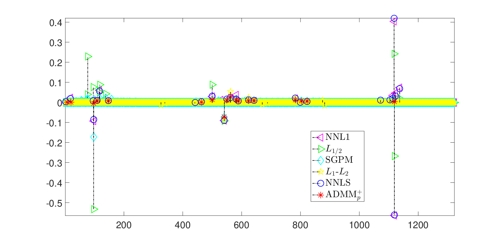
Tables 3 and 4 show the errors ( ${\tt err}=\|{\hat{\mathbf{x}}}-{\mathbf{x}}^{*}\|_{2}$ ) between the reconstructed vectors and the ground-truth, and computational time (Time (s)) under different amounts of noise, respectively. Each recorded value is the average of $20$ random realizations. In Fig. 2, the ground truth and the error vectors of these comparing algorithms defined by the constructed signals minus the true signal are presented in Plots (a) and (b), for the scenario of ${\tt std}=0.05$ . The horizontal heavy yellow line surrounded by cyan is caused by the full-dimension error vectors from $L_{1}$ - $L_{2}$ , SGPM, NNL1, $L_{1/2}$ . The deviation of ADMM ${}_{p}^{+}$ is much smaller than the others. ADMM ${}_{p}^{+}$ achieves the best recovery quality in the sense of highest accuracy and sparsity. All the results demonstrate that ADMM ${}_{p}^{+}$ is comparable to NNLS in terms of accuracy for noiseless data, and even more accurate than NNLS for noisy cases. In comparison with NNL1, $L_{1}$ - $L_{2}$ , ADMM ${}_{p}^{+}$ also ends up with much higher accuracy and takes less time. In contrast with $L_{1/2}$ , ADMM ${}_{p}^{+}$ converges to a much more accurate solution while consuming a bit more time. Besides, for solving the same $(L_{1}/L_{2})^{+}$ model, ADMM ${}_{p}^{+}$ costs significantly less time than SGPM while still achieving a much more accurate solution. More specificially, ADMM ${}_{p}^{+}$ reduces computational time by about $95\%\sim 99\%$ compared to SGPM.

Table 3: Reconstructed error (

{\tt err}=\|{\hat{\mathbf{x}}}-{\mathbf{x}}^{*}\|_{2}

) for DOAS.

std	NNLS	NNL1	$L_{1}$ - $L_{2}$	$L_{1/2}$	$(L_{1}/L_{2})^{+}$
					ADMM ${}_{p}^{+}$	SGPM
0	7.72e-16	2.70e-03	5.21e-05	3.60e-03	2.58e-05	4.80e-02
0.001	4.91e-03	7.95e-03	8.76e-04	2.41e-02	4.37e-04	7.60e-02
0.005	3.26e-02	1.92e-02	3.05e-03	6.95e-02	2.03e-03	3.75e-01
0.01	1.46e-01	1.61e-01	4.90e-03	1.04e-01	4.25e-03	3.84e-01
0.05	1.73e-01	1.75e-01	2.39e-02	1.30e-01	2.00e-02	5.67e-01

Table 4: Computational time (s) for DOAS under different noisy level.

std	NNLS	NNL1	$L_{1}$ - $L_{2}$	$L_{1/2}$	$(L_{1}/L_{2})^{+}$
					ADMM ${}_{p}^{+}$	SGPM
0	0.021	8.05	13.30	0.10	5.66	3110.00
0.001	0.047	8.19	35.60	0.11	6.59	3030.00
0.005	0.016	7.77	28.10	0.13	7.17	437.00
0.01	0.057	8.50	33.90	0.13	8.34	167.00
0.05	0.052	8.82	70.90	0.13	4.00	276.00

6 Conclusions

We carry out a unified theoretical study on both $L_{1}/L_{2}$ minimization models, including the constrained and the unconstrained. First, we prove that the existence of the globally optimal solution can be guaranteed by the $\mu$ -spherical section property of the null space of the matrix $A$ . Second, we analyze the sparsity property of the constrained and the unconstrained models. Third, we derive a closed-form solution of the proximal operator of $\left(L_{1}/L_{2}\right)^{+}$ . Equipped with this, we propose a specific splitting scheme (ADMM ${}_{p}^{+}$ ) to solve the unconstrained $\left(L_{1}/L_{2}\right)^{+}$ model. We establish its global convergence to a d-stationary solution by verifying the KL property of the merit function. Numerical simulations validate our analyses and demonstrate that ADMM ${}_{p}^{+}$ outperforms other state-of-the-art methods in sparse recovery.

Funding Min Tao was partially supported by National Key Research and Development Program of China (2018AAA0101100), the Natural Science Foundation of China (No. 11971228) and Jiangsu University QingLan Project. The work of Xiao-Ping Zhang is supported by the Natural Sciences and Engineering Research Council of Canada (NSERC), Grant No. RGPIN-2020-04661.
Data Availibility The datasets generated during and/or analysed during the current study are available from the corresponding author on reasonable request.
Declarations Conflict of interests The authors have no relevant financial or non-financial interests to disclose.

References

(1) H. Attouch, J. Bolte, and B. F. Svaiter, Convergence of descent methods for semi-algebraic and tame problems: proximal algorithms, forward-backward splitting, and regularized Gauss-Seidel methods, Math. Program., 146 (2014), pp. 459–494.
(2) J. Bochnak, M. Coste, and M.-F. Roy, Real Algebraic Geometry, Ergeb. Math. Grenzgeb. 36, Springer-Verlag, Berlin, 1998.
(3) J. Bolte, A. Daniilidis, and A. Lewis, The Łojasiewicz inequality for nonsmooth subanalytic functions with applications to subgradient dynamical systems, SIAM J. Optim., 17 (2007), pp. 1205–1223.
(4) K. Bredies, D. A. Lorenz, and S. Reiterer, Minimization of non-smooth, non-convex functionals by iterative thresholding, J. Optim. Theory Appl., 165 (2015), pp. 78–112.
(5) E. Candes and T. Tao, Decoding by linear programming, IEEE Trans. Inform. Theory, 51 (2005), pp. 4203–4215.
(6) R. Chartrand, Exact reconstruction of sparse signals via nonconvex minimization, IEEE Signal Process Lett., 14 (2007), pp. 707–710.
(7) S. S. Chen, D. L. Donoho, and M. A. Saunders, Atomic decomposition by basis pursuit, SIAM J. Sci. Comput., 20 (1998), pp. 33–61.
(8) F. H. Clarke, Optimization and Nonsmooth Analysis, vol. 5, Classical Appl. Math. Society for Industrial and Applied Mathematics, Philadelphia, PA, 1990.
(9) A. Cohen, W. Dahmen, and R. Devore, Compressed sensing and best $k$ -term approximation, J. Am. Math. Soc., 22 (2009), pp. 211–231.
(10) H. Dong and M. Tao, On the linear convergence to weak/standard D-stationary points of DCA-based algorithms for structured nonsmooth DC programming, J. Optim. Theory Appl., 189 (2021), pp. 190–220.
(11) E. Esser, Y. Lou, and J. Xin, A method for finding structured sparse solutions to nonnegative least squares problems with applications, SIAM J. Imaging Sci., 6 (2013), pp. 2010–2046.
(12) A. Fannjiang and W. Liao, Coherence-pattern-guided compressive sensing with unresolved grids, SIAM J. Imaging Sci., 5 (2012), pp. 179–202.
(13) B. Finlayson-Pitts, Unpublished data, (2000). Provided by Wingen, L. M.
(14) P. Gong, C. Zhang, Z. Lu, J. Z. Huang, and J. Ye, A general iterative shrinkage and thresholding algorithm for non-convex regularized optimization problems, JMLR workshop and conference proceedings, 28 (2013), pp. 37–45.
(15) A. J. Hoffman, On approximate solutions of systems of linear inequalities, J. Res. Nat. Bur. Standards, 49 (1952), pp. 263–265.
(16) M. Y. Hong, Z. Q. Luo, and M. Razaviyayn, Convergence analysis of alternating direction method of multipliers for a family of nonconvex problems, SIAM J. Optim., 26 (2016), pp. 337–364.
(17) P. O. Hoyer, Non-negative sparse coding, in Proc. IEEE Workshop on Neural Networks for Signal Processing, 2002, pp. 557–565.
(18) N. Hurley and S. Rickard, Comparing measures of sparsity, IEEE Trans. Inform. Theory, 55 (2009), pp. 4723–4741.
(19) H. Ji, J. Li, Z. Shen, and K. Wang, Image deconvolution using a characterization of sharp images in wavelet domain, Appl. Comput. Harmon. Anal., 32 (2012), pp. 295–304.
(20) M. J. Lai, Y. Xu, and W. Yin, Improved iteratively reweighted least squares for unconstrained smoothed $\ell_{q}$ minimization, SIAM J. Numer. Anal., 51 (2013), pp. 927–957.
(21) G. Y. Li and T. K. Pong, Global convergence of splitting methods for nonconvex composite optimization, SIAM J. Optim., 25 (2015), pp. 2434–2460.
(22) H. Li and Z. Lin, in Advances in Neural Information Processing Systems, C. Cortes, N. Lawrence, D. Lee, M. Sugiyama, and R. Garnett, eds.
(23) J. Li, A. M.-C. So, and W.-K. Ma, Understanding notions of stationarity in nonsmooth optimization: A guided tour of various constructions of subdifferential for nonsmooth functions, IEEE Signal Proc. Mag., 37 (2020), pp. 18–31.
(24) Y. Lou, S. Osher, and J. Xin, Computational aspects of constrained ${L}_{1}$ - ${L}_{2}$ minimization for compressive sensing, in Model. Comput. $\&$ Optim. Inf. Syst. $\&$ Manage. Sci., Advances in Intelligent Systems and Computing, vol. 359, 2015, pp. 169–180.
(25) Y. Lou and M. Yan, Fast L1-L2 minimization via a proximal operator, J. Sci. Comput., 74 (2018), pp. 767–785.
(26) M. Morup, K. H. Madsen, and L. K. Hansen, Approximate $l_{0}$ constrained non-negative matrix and tensor factorization, in ISCAS, 2008, pp. 1328–1331.
(27) S. Nakayama and J. Y. Gotoh, On the superiority of pgms to pdcas in nonsmooth nonconvex sparse regression, Optim. Lett., 15 (2021), pp. 2831–2860.
(28) B. K. Natarajan, Sparse approximate solutions to linear systems, SIAM J. Comput., 24 (1995), pp. 227–234.
(29) M. Nikolova, Local strong homogeneity of a regularized estimator, SIAM J. Math. Anal., 61 (2000), pp. 633–658.
(30) J. S. Pang, M. Razaviyayn, and A. Alvarado, Computing B-stationary points of nonsmooth DC programs, Math. Oper. Res., 42 (2017), pp. 95–118.
(31) Y. Rahimi, C. Wang, H. Dong, and Y. Lou, A scale-invariant approach for sparse signal recovery, SIAM J. Sci. Comput., 41 (2019), pp. A3649–A3672.
(32) A. Repetti, M. Q. Pham, L. Duval, E. Chouzenoux, and J. C. Pesquet, Euclid in a taxicab: Sparse blind deconvolution with smoothed ${\ell_{1}}/{\ell_{2}}$ regularization, IEEE Signal Process Lett., 22 (2015), pp. 539–543.
(33) R. T. Rockafellar and R. J. B. Wets, Variational analysis, 1998.
(34) M. Tao, Minimization of L₁ over L₂ for sparse signal recovery with convergence guarantee, SIAM J. Sci. Comput., 44 (2022), pp. A770–A797.
(35) S. A. Vavasis, Derivation of compressive sensing theorems from the spherical section property, University of Waterloo, (2009).
(36) C. Wang, M. Yan, Y. Rahimi, and Y. Lou, Accelerated schemes for the L₁/L₂ minimization, IEEE Trans. Signal Process., 68 (2020), pp. 2660–2669.
(37) Y. Wang, W. Yin, and J. Zeng, Global convergence of ADMM in nonconvex nonsmooth optimization, J. Sci. Comput., 78 (2019), pp. 1–35.
(38) P. Yin, E. Esser, and J. Xin, Ratio and difference of $\ell_{1}$ and $\ell_{2}$ norms and sparse representation with coherent dictionaries, Comm. Info. Systems, 14 (2014), pp. 87–109.
(39) L. Y. Zeng, P. R. Yu, and T. K. Pong, Analysis and algorithms for some compressed sensing models based on L1/L2 minimization, SIAM J. Optim., 31 (2021), pp. 1576–1603.

Success rates	Success rates

Algorithm failures	Algorithm failures

Model failures	Model failures

Unified Analysis on L1L_{1} over L2L_{2} Minimization for signal recovery

Abstract

Keywords:

MSC

1 Preliminary

Definition 1

Definition 2

Definition 3

Definition 4

2 Existence of optimal solutions

Lemma 1

Proof

Proposition 1

Proof

Theorem 2.1

Proof

Corollary 1

Proof

Theorem 2.2

Proof

Theorem 2.3

Theorem 2.4

Proof

Remark 1

3 Sparse property

Theorem 3.1

Proof

Theorem 3.2

Proof

Remark 2

Lemma 2

Proof

Corollary 2

Proof

Theorem 3.3

4 Computational approach

4.1 Proximal operator

Theorem 4.1

Proof

4.2 ADMM for solving (5) with 𝒳=ℝ+n{\cal X}=\mathbb{R}_{+}^{n}

4.3 Global Convergence

Lemma 3

Proof

Lemma 4

Proof

Theorem 4.2

Theorem 4.3

Proof

5 Numerical results

5.1 Algorithmic behaviors

5.2 Comparison on various models

5.3 Recovery of nonnegative signal from coherent dictionaries

5.4 DOAS

6 Conclusions

References

Unified Analysis on $L_{1}$ over $L_{2}$ Minimization for signal recovery

4.2 ADMM for solving (5) with ${\cal X}=\mathbb{R}_{+}^{n}$