跳到论文正文
W Papers独立论文阅读器 arXiv:2108.01244 论文正文 计算阅读时间 · 0%
引用这篇论文根据当前论文元数据生成,正式投稿前建议核对。


License: arXiv.org perpetual non-exclusive license
arXiv:2108.01244v2 [math.AP] 31 Dec 2022

Level-set forced mean curvature flow with the Neumann boundary conditionThanks:  The work of JJ was partially supported by NSF CAREER grant DMS-1843320. The work of HM was partially supported by the JSPS grants: KAKENHI #19K03580, #19H00639, #17KK0093, #20H01816. The work of HT was partially supported by NSF CAREER grant DMS-1843320 and a Simons Fellowship.

Jiwoong Jang Jiwoong Jang Department of Mathematics, University of Wisconsin Madison, Van Vleck hall, 480 Lincoln drive, Madison, WI 53706, USA Email address: jjang57@wisc.edu , Dohyun Kwon Dohyun Kwon Department of Mathematics, University of Wisconsin Madison, Van Vleck hall, 480 Lincoln drive, Madison, WI 53706, USA Email address: dkwon7@wisc.edu , Hiroyoshi Mitake H. Mitake Graduate School of Mathematical Sciences, University of Tokyo 3-8-1 Komaba, Meguro-ku, Tokyo, 153-8914, Japan Email address: mitake@g.ecc.u-tokyo.ac.jp and Hung V. Tran Hung V. Tran Department of Mathematics, University of Wisconsin Madison, Van Vleck hall, 480 Lincoln drive, Madison, WI 53706, USA Email address: hung@math.wisc.edu
Date: August 11, 2026
Abstract.

Here, we study a level-set forced mean curvature flow with the homogeneous Neumann boundary condition. We first show that the solution is Lipschitz in time and locally Lipschitz in space. Then, under an additional condition on the forcing term, we prove that the solution is globally Lipschitz. We obtain the large time behavior of the solution in this setting and study the large time profile in some specific situations. Finally, we give two examples demonstrating that the additional condition on the forcing term is sharp, and without it, the solution might not be globally Lipschitz.

Key words and phrases: 
Level-set forced mean curvature flows; Neumann boundary problem; global Lipschitz regularity; large time behavior; the large time profile
2010 Mathematics Subject Classification
35B40, 49L25, 53E10, 35B45, 35K20, 35K93,

1. Introduction

In this paper, we study the level-set equation for the forced mean curvature flow

ut=|D​u​|div⁡(D​u|D​u|)+c⁡(x)|​D​u|\displaystyle u_{t}=|Du|\operatorname{div}\left(\frac{Du}{|Du|}\right)+c(x)|Du| in Ω×(0,∞)\Omega\times(0,\infty), (1.1)
∂u∂𝐧→=0\displaystyle\displaystyle\frac{\partial u}{\partial\vec{\mathbf{n}}}=0 on ∂Ω×[0,∞)\partial\Omega\times[0,\infty), (1.2)
u​(x,0)=u0​(x)\displaystyle u(x,0)=u_{0}(x) on Ω¯\overline{\Omega}. (1.3)

The domain Ω⊂ℝn\Omega\subset\mathbb{R}^{n} with n≥2n\geq 2 is assumed to be bounded and C2,θC^{2,\theta} for some θ∈(0,1)\theta\in(0,1). Here, c=c⁡(x)c=c(x) is a forcing function, which is in C1​(Ω¯)C^{1}(\overline{\Omega}), and 𝐧→\vec{\mathbf{n}} is the outward unit normal vector to ∂Ω\partial\Omega. Throughout this paper, we assume that u0∈C2,θ​(Ω¯)u_{0}\in C^{2,\theta}(\overline{\Omega}), and ∂u0∂𝐧→=0​on​∂Ω\frac{\partial u_{0}}{\partial\vec{\mathbf{n}}}=0\ \text{on}\ \partial\Omega for compatibility.

We first notice that the well-posedness and the comparison principle for (1.1)–(1.3) are well established in the theory of viscosity solutions (see [4, 2, 10, 11] for instance). Our main interest in this paper is to go beyond the well-posedness theory to understand the Lipschitz regularity and large time behavior of the solution. The Lipschitz regularity for the solution is rather subtle because of the competition between the forcing term and the mean curvature term together with the constraint on perpendicular intersections of the level sets of the solution with the boundary of Ω\Omega. It is worth emphasizing that the geometry of ∂Ω\partial\Omega plays a crucial role in the analysis.

We now describe our main results. First of all, we show that uu is Lipschitz in time and locally Lipschitz in space.

Theorem 1.1.

Let uu be the unique viscosity solution uu of (1.1)–(1.3). Then, there exists a constant M>0M>0 and for each T>0T>0, there exists a constant CT>0C_{T}>0 depending on TT such that

{|u⁡(x,t)−u⁡(x,s)|⩽M​|t−s|,|u⁡(x,t)−u⁡(y,t)|⩽CT​|x−y|, for all x,y∈Ω¯, t,s∈[0,T].\begin{cases}|u(x,t)-u(x,s)|\leqslant M|t-s|,\\ |u(x,t)-u(y,t)|\leqslant C_{T}|x-y|,\end{cases}\quad\text{ for all $x,y\in\overline{\Omega}$, $t,s\in[0,T]$.}

We next show that if we put some further conditions on the forcing term cc, then we have the global Lipschitz estimate in xx of the solution. Denote by

{C0:=max⁡{−λ:λ​is a principal curvature of ∂Ω at x0 for x0∈∂Ω}∈ℝ,K0:=min⁡{d:d​is the diameter of an open ball inscribed in​Ω}>0.\begin{cases}C_{0}:=\max\{-\lambda\,:\,\lambda\ \textrm{is a principal curvature of $\partial\Omega$ at $x_{0}$ for $x_{0}\in\partial\Omega$}\}\in\mathbb{R},\\ K_{0}:=\min\{d\,:\,d\ \textrm{is the diameter of an open ball inscribed in}\ \Omega\}>0.\end{cases}
Theorem 1.2.

Assume that there exists δ>0\delta>0 such that

1n​c​(x)2−|D​c​(x)|−δ>max⁡{0,C0​|c⁡(x)|+2​n​C0K0}for all​x∈Ω.\frac{1}{n}c(x)^{2}-|Dc(x)|-\delta>\max\left\{0,\ C_{0}|c(x)|+\frac{2nC_{0}}{K_{0}}\right\}\quad\text{for all}\ x\in\Omega. (1.4)

Let uu be the unique viscosity solution to (1.1)–(1.3). Then, there exist constants M,L>0M,L>0 depending only on the forcing term cc and the initial data u0u_{0} such that

{|u⁡(x,t)−u⁡(x,s)|⩽M​|t−s|,|u⁡(x,t)−u⁡(y,t)|⩽L​|x−y|, for all x,y∈Ω¯, t,s∈[0,∞).\begin{cases}|u(x,t)-u(x,s)|\leqslant M|t-s|,\\ |u(x,t)-u(y,t)|\leqslant L|x-y|,\end{cases}\quad\text{ for all $x,y\in\overline{\Omega}$, $t,s\in[0,\infty)$.} (1.5)

Let us now explain a bit the geometric meaning of K0K_{0}. For each x∈∂Ωx\in\partial\Omega, let

Kx=max⁡{2​r>0:B⁡(x−r​𝐧→​(x),r)⊂Ω}.K_{x}=\max\{2r>0\,:\,B(x-r\vec{\mathbf{n}}(x),r)\subset\Omega\}.

Then, K0=minx∈∂Ω⁡KxK_{0}=\min_{x\in\partial\Omega}K_{x}. We notice next that if Ω\Omega is convex in Theorem 1.2, then we clearly have C0≤0C_{0}\leq 0. In this case, (1.4) becomes 1n​c​(x)2−|D​c​(x)|−δ>0\frac{1}{n}c(x)^{2}-|Dc(x)|-\delta>0, a kind of coercive assumption, which often appears in the usage of the classical Bernstein method to obtain Lipschitz regularity (see [19] for instance).

In the specific case where c≡0c\equiv 0 and Ω\Omega is convex and bounded, the global Lipschitz estimate of the solution was obtained in [9]. See Remark 1. Moreover, a very interesting example was given in [9] to show that the solution is not globally Lipschitz continuous if Ω\Omega is not convex. Motivated by this example, we give two examples showing that uu is not globally Lipschitz continuous if we do not impose (1.4). Furthermore, the examples demonstrate that condition (1.4) is sharp.

Let us note that the graph mean curvature flow with the Neumann boundary conditions has been studied much in the literature (see [15, 13, 20] and the references therein).

We next study the large time behavior of uu under condition (1.4).

Theorem 1.3.

Assume (1.4). Let uu be the unique viscosity solution to (1.1)–(1.3). Then,

u⁡(⋅,t)→v, as ​t→∞,u(\cdot,t)\rightarrow v,\quad\text{ as }t\rightarrow\infty,

uniformly on Ω¯\overline{\Omega} for some Lipschitz function vv, which is a viscosity solution to

{−(div⁡(D​v|D​v|)+c⁡(x))​|D​v|=0in​Ω,∂v∂𝐧→=0on​∂Ω.\begin{cases}-\left(\operatorname{div}\left(\frac{Dv}{|Dv|}\right)+c(x)\right)|Dv|=0\quad\ &{\rm in}\ \Omega,\\ \displaystyle\frac{\partial v}{\partial\vec{\mathbf{n}}}=0\quad\ &{\rm on}\ \partial\Omega.\end{cases} (1.6)

We prove Theorem 1.3 by using a Lyapunov function, which is quite standard. We say that vv is the large time profile of the solution uu. It is important to note that the stationary problem (1.6) may have various different solutions, and thus, the question on how the large time profile vv depends on the initial data u0u_{0} is rather delicate and challenging. We are able to answer this question in the radially symmetric setting, and it is still widely open in the general settings.

Theorem 1.4.

Suppose that, by abuse of notions,

{Ω=B⁡(0,R)​ for some ​R>0,c⁡(x)=c⁡(r)​ for ​|x|=r∈[0,R],u0​(x)=u0​(r)​ for ​|x|=r∈[0,R].\begin{cases}\Omega=B(0,R)\text{ for some }R>0,\\ c(x)=c(r)\text{ for }|x|=r\in[0,R],\\ u_{0}(x)=u_{0}(r)\text{ for }|x|=r\in[0,R].\end{cases} (1.7)

Here, c∈C1​([0,R],[0,∞))c\in C^{1}([0,R],[0,\infty)), and u0∈C2​([0,R])u_{0}\in C^{2}([0,R]) with u0′​(R)=0u_{0}^{\prime}(R)=0. Denote by

𝒜:={r∈(0,R]:c⁡(r)=n−1r},\displaystyle\mathcal{A}:=\left\{r\in(0,R]\,:\,c(r)=\frac{n-1}{r}\right\},
𝒜+:={r∈(0,R]:c⁡(r)>n−1r},\displaystyle\mathcal{A}_{+}:=\left\{r\in(0,R]\,:\,c(r)>\frac{n-1}{r}\right\},
𝒜−:={r∈(0,R]:c⁡(r)<n−1r}.\displaystyle\mathcal{A}_{-}:=\left\{r\in(0,R]\,:\,c(r)<\frac{n-1}{r}\right\}.

Define d:(0,R]→(0,R]d:(0,R]\to(0,R] as

d⁡(r)={r if ​r∈𝒜,max⁡(𝒜∩(0,r)) if ​r∈𝒜+,min⁡(𝒜∩(r,R]) if ​r∈𝒜−​ and ​𝒜∩(r,R]≠∅,R if ​r∈𝒜−​ and ​𝒜∩(r,R]=∅.d(r)=\begin{cases}r\qquad&\text{ if }r\in\mathcal{A},\\ \max\left(\mathcal{A}\cap(0,r)\right)\qquad&\text{ if }r\in\mathcal{A}_{+},\\ \min\left(\mathcal{A}\cap(r,R]\right)\qquad&\text{ if }r\in\mathcal{A}_{-}\text{ and }\mathcal{A}\cap(r,R]\neq\emptyset,\\ R\qquad&\text{ if }r\in\mathcal{A}_{-}\text{ and }\mathcal{A}\cap(r,R]=\emptyset.\end{cases}

Write u⁡(x,t)=ϕ⁡(|x|,t)u(x,t)=\phi(|x|,t) for x∈Ω=B⁡(0,R)x\in\Omega=B(0,R) and t⩾0t\geqslant 0. Then, the limiting profile ϕ∞​(r)=limt→∞ϕ⁡(r,t)\phi_{\infty}(r)=\lim_{t\to\infty}\phi(r,t) can be written in terms of u0u_{0} as: for each r0∈(0,R]r_{0}\in(0,R],

ϕ∞​(r0)=max⁡{u0​(r):r⩾d⁡(r0)}.\phi_{\infty}(r_{0})=\max\left\{u_{0}(r)\,:\,r\geqslant d(r_{0})\right\}. (1.8)

As a by-product, Theorem 1.4 shows that the solution to (1.1)–(1.3) is not globally Lipschitz continuous with an appropriate choice of initial data u0u_{0}.

Corollary 1.5.

Consider the setting in Theorem 1.4. Assume that there exist 0<a<b<R0<a<b<R such that a,b∈𝒜a,b\in\mathcal{A} and (a,b)⊂𝒜−(a,b)\subset\mathcal{A}_{-}. Assume further that u0u_{0} is a C2C^{2} function on [0,R][0,R] such that

u0​(r)={1 for ​r⩽a,∈(0,1) for ​a<r⩽b,0 for ​b<r⩽R.u_{0}(r)=\begin{cases}1\quad&\text{ for }r\leqslant a,\\ \in(0,1)\quad&\text{ for }a<r\leqslant b,\\ 0\quad&\text{ for }b<r\leqslant R.\end{cases}

Then, uu is not globally Lipschitz, and

ϕ∞​(r)={1 for ​r⩽a,0 for ​a<r⩽R.\phi_{\infty}(r)=\begin{cases}1\quad&\text{ for }r\leqslant a,\\ 0\quad&\text{ for }a<r\leqslant R.\end{cases}

Lastly, we give another example to show the non global Lipschitz phenomenon in Theorem 6.1. Since we deal with the situation where Ω\Omega is unbounded there, we leave the precise statement of Theorem 6.1 and corresponding adjustments to Section 6.

Our problem (1.1)–(1.2) basically describes a level-set forced mean curvature flow with the homogeneous Neumann boundary condition. If a level set of the unknown uu is a smooth enough surface, then it evolves with the normal velocity V⁡(x)=κ+c⁡(x)V(x)=\kappa+c(x), where κ\kappa equals (n−1)(n-1) times the mean curvature of the surface at xx, and it perpendicularly intersects ∂Ω\partial\Omega (if ever). What is really interesting and delicate here is the competition between the forcing term c⁡(x)c(x) and the mean curvature term κ\kappa coupled with the constraint on perpendicular intersections of the level sets with the boundary. It is worth emphasizing that we do not assume Ω\Omega is convex, and the geometry of ∂Ω\partial\Omega plays a crucial role in the behavior of the solution here. Indeed, analyzing the competition between the two constraints, the force and the boundary condition subjected to ∂Ω\partial\Omega, as time evolves in viscosity sense is the main topic of this paper.

We now briefly describe our approaches to get the aforementioned results. We use the maximum principle and rely on the classical Bernstein method to establish a priori gradient estimates for the solution. The main difficulty is when a maximizer is located on the boundary, which we cannot apply the maximum principle directly. We deal with this difficulty by considering a multiplier that puts the maximizer, with the homogeneous Neumann boundary condition, inside the domain so that the maximum principle is applicable. To the best of our knowledge, the idea of handling a maximizer in the proof of Theorem 1.2 for the level-set equation for forced mean curvature flows under the Neumann boundary condition is new in the literature.

Once we get a global Lipschitz estimate for the solution, by using a standard Lyapunov function, we prove the convergence in Theorem 1.3. Next, the radially symmetric setting is considered, and (1.1)–(1.3) are reduced to a first-order singular Hamilton-Jacobi equation with the homogeneous Neumann boundary condition; see [7, 8] for a related problem on the whole space. By using the representation formula for the Neumann problem (see, e.g., [16]), we are able to obtain Theorem 1.4 and Corollary 1.5. The situation considered in Theorem 6.1 is related to that in [23, Section 4] with no forcing term. As we have a constant forcing cc interacting with the boundary, the construction in the proof of Theorem 6.1 is rather delicate and involved. It is worth emphasizing that Corollary 1.5 and Theorem 6.1 demonstrate that condition (1.4), which is needed for the global Lipschitz regularity of uu, is essentially optimal.

We conclude this introduction by giving a non exhaustive list of related works to our paper. There are several asymptotic analysis results on the forced mean curvature flows with Neumann boundary conditions [13, 21, 22, 24] or with periodic boundary conditions [3], but they are all for graph-like surfaces. The volume preserving mean curvature flow, which is a different type of forced mean curvature flows, was studied in [17, 18]. Recently, the relation between the level set approach and the varifold approach for (1.1) with c≡0c\equiv 0 was investigated in [1]. We also refer to [8, 14] for some recent results on the asymptotic growth speed of solutions to forced mean curvature flows with discontinuous source terms in the whole space.

Organization of the paper

The paper is organized as follows. In Section 2, we give the notion of viscosity solutions to the problem and some basic results. In Section 3, we prove the local and global gradient estimates. Section 4 is devoted to the study on large time behavior of the solution and its large time profile. We give two examples that the spatial gradient of the solution grows to infinity as time tends to infinity in Sections 5 and 6 if we do not impose assumption (1.4) on the force cc.

2. Preliminaries

In this section, we recall the notion of viscosity solutions to the Neumann boundary problem (1.1)–(1.3) and give some related results.

Let 𝒮n\mathcal{S}^{n} be the set of symmetric matrices of size nn. Define F:Ω¯×(ℝn∖{0})×𝒮n→ℝF:\overline{\Omega}\times(\mathbb{R}^{n}\setminus\{0\})\times\mathcal{S}^{n}\rightarrow\mathbb{R} by

F⁡(x,p,X)=trace​((I−p⊗p|p|2)​X)+c⁡(x)​|p|.F(x,p,X)=\text{trace}\left(\left(I-\frac{p\otimes p}{|p|^{2}}\right)X\right)+c(x)|p|.

We denote the semicontinuous envelopes of FF by, for (x,p,X)∈Ω¯×ℝn×𝒮n(x,p,X)\in\overline{\Omega}\times\mathbb{R}^{n}\times\mathcal{S}^{n},

F∗​(x,p,X)=lim inf(y,q,Y)→(x,p,X)F⁡(y,q,Y),F∗​(x,p,X)=lim sup(y,q,Y)→(x,p,X)F⁡(y,q,Y).F_{*}(x,p,X)=\liminf_{(y,q,Y)\rightarrow(x,p,X)}F(y,q,Y),\quad F^{*}(x,p,X)=\limsup_{(y,q,Y)\rightarrow(x,p,X)}F(y,q,Y).
Definition 2.1.

An upper semicontinuous function u:Ω¯×[0,∞)→ℝu:\overline{\Omega}\times[0,\infty)\rightarrow\mathbb{R} is said to be a viscosity subsolution of (1.1)–(1.3) if u⁡(⋅,0)⩽u0u(\cdot,0)\leqslant u_{0} on Ω¯\overline{\Omega}, and, for any φ∈C2​(Ω¯×[0,∞))\varphi\in C^{2}(\overline{\Omega}\times[0,\infty)), if (x^,t^)∈Ω¯×(0,∞)(\hat{x},\hat{t})\in\overline{\Omega}\times(0,\infty) is a maximizer of u−φu-\varphi, and if x^∈Ω\hat{x}\in\Omega, then

φt​(x^,t^)−F∗​(x^,D​φ​(x^,t^),D2​φ​(x^,t^))⩽0;\varphi_{t}(\hat{x},\hat{t})-F^{*}(\hat{x},D\varphi(\hat{x},\hat{t}),D^{2}\varphi(\hat{x},\hat{t}))\leqslant 0;

if x^∈∂Ω\hat{x}\in\partial\Omega, then

min⁡{φt​(x^,t^)−F∗​(x^,D​φ​(x^,t^),D2​φ​(x^,t^)),∂φ∂𝐧→​(x^,t^)}⩽0.\min\left\{\varphi_{t}(\hat{x},\hat{t})-F^{*}(\hat{x},D\varphi(\hat{x},\hat{t}),D^{2}\varphi(\hat{x},\hat{t})),\frac{\partial\varphi}{\partial\vec{\mathbf{n}}}(\hat{x},\hat{t})\right\}\leqslant 0.

Similarly, a lower semicontinuous function u:Ω¯×[0,∞)→ℝu:\overline{\Omega}\times[0,\infty)\rightarrow\mathbb{R} is said to be a viscosity supersolution of (1.1)–(1.3) if u⁡(⋅,0)⩾u0u(\cdot,0)\geqslant u_{0} on Ω¯\overline{\Omega}, and, for any φ∈C2​(Ω¯×[0,∞))\varphi\in C^{2}(\overline{\Omega}\times[0,\infty)), if (x^,t^)∈Ω¯×(0,∞)(\hat{x},\hat{t})\in\overline{\Omega}\times(0,\infty) is a minimizer of u−φu-\varphi, and if x^∈Ω\hat{x}\in\Omega, then

φt​(x^,t^)−F∗​(x^,D​φ​(x^,t^),D2​φ​(x^,t^))⩾0;\varphi_{t}(\hat{x},\hat{t})-F_{*}(\hat{x},D\varphi(\hat{x},\hat{t}),D^{2}\varphi(\hat{x},\hat{t}))\geqslant 0;

if x^∈∂Ω\hat{x}\in\partial\Omega, then

max⁡{φt​(x^,t^)−F∗​(x^,D​φ​(x^,t^),D2​φ​(x^,t^)),∂φ∂𝐧→​(x^,t^)}⩾0.\max\left\{\varphi_{t}(\hat{x},\hat{t})-F_{*}(\hat{x},D\varphi(\hat{x},\hat{t}),D^{2}\varphi(\hat{x},\hat{t})),\frac{\partial\varphi}{\partial\vec{\mathbf{n}}}(\hat{x},\hat{t})\right\}\geqslant 0.

Finally, a continuous function uu is said to be a viscosity solution of (1.1)–(1.3) if uu is both its viscosity subsolution and its viscosity supersolution.

Henceforth, since we are always concerned with viscosity solutions, the adjective “viscosity” is omitted. The following comparison principle for solutions to (1.1)–(1.3) in a bounded domain is well known (see, e.g., [10]).

Proposition 2.2 (Comparison principle for (1.1)–(1.3)).

Let uu and vv be a subsolution and a supersolution of (1.1)–(1.3), respectively. Then, u⩽vu\leqslant v in Ω¯×[0,∞)\overline{\Omega}\times[0,\infty).

To obtain Lipschitz estimates, it is convenient to consider an approximate problem of (1.1)–(1.3) by considering, for ε>0\varepsilon>0, T>0T>0,

{utε=ε2+|D​uε|2​div​(D​uεε2+|D​uε|2)+c⁡(x)​ε2+|D​uε|2 in ​Ω×(0,T],∂uε∂𝐧→=0 on ​∂Ω×[0,T],uε​(x,0)=u0​(x) on ​Ω¯.\begin{cases}u^{\varepsilon}_{t}=\sqrt{\varepsilon^{2}+|Du^{\varepsilon}|^{2}}\,\text{div}\left(\frac{Du^{\varepsilon}}{\sqrt{\varepsilon^{2}+|Du^{\varepsilon}|^{2}}}\right)+c(x)\sqrt{\varepsilon^{2}+|Du^{\varepsilon}|^{2}}\quad&\text{ in }\Omega\times(0,T],\\ \displaystyle\frac{\partial u^{\varepsilon}}{\partial\vec{\mathbf{n}}}=0\quad&\text{ on }\partial\Omega\times[0,T],\\ u^{\varepsilon}(x,0)=u_{0}(x)\quad&\text{ on }\overline{\Omega}.\end{cases} (2.1)

Equation (2.1) describes the motion of the graph of uεε\frac{u^{\varepsilon}}{\varepsilon} under the forced mean curvature flow V=κ+cV=\kappa+c in Ω\Omega with right contact angle condition on ∂Ω\partial\Omega. The following result on a priori estimates on the gradient of uεu^{\varepsilon} plays a crucial role in our analysis.

Theorem 2.3 (A priori estimates).

Assume that ∂Ω\partial\Omega is smooth and c∈C∞​(Ω¯)c\in C^{\infty}(\overline{\Omega}). For each ε∈(0,1)\varepsilon\in(0,1) and T>0T>0, assume that uε∈C∞​(Ω¯×(0,T])∩C1​(Ω¯×[0,T])u^{\varepsilon}\in C^{\infty}(\overline{\Omega}\times(0,T])\cap C^{1}(\overline{\Omega}\times[0,T]) is the unique solution of (2.1). Then, there exist a constant M>0M>0 and a constant CT>0C_{T}>0 depending on TT such that

∥utε∥L∞​(Ω¯×[0,T])⩽M and ∥D​uε∥L∞​(Ω¯×[0,T])⩽CT.\lVert u^{\varepsilon}_{t}\rVert_{L^{\infty}(\overline{\Omega}\times[0,T])}\leqslant M\quad\text{ and }\quad\lVert Du^{\varepsilon}\rVert_{L^{\infty}(\overline{\Omega}\times[0,T])}\leqslant C_{T}. (2.2)

Here, MM and CTC_{T} are independent of ε∈(0,1)\varepsilon\in(0,1).

The proof of Theorem 2.3 is given in the next section. The a priori estimates then allow us to get the existence and uniqueness of solutions to (2.1).

Proposition 2.4.

For each ε∈(0,1)\varepsilon\in(0,1) and T>0T>0, equation (2.1) has a unique continuous solution uεu^{\varepsilon}. Furthermore, uε∈C2,1​(Ω×(0,T])∩C1​(Ω¯×[0,T])u^{\varepsilon}\in C^{2,1}(\Omega\times(0,T])\cap C^{1}(\overline{\Omega}\times[0,T]) and (2.2) holds.

Proposition 2.4 can be obtained by the classical parabolic PDE theory. For instance, we refer to [22] for a similar form of Proposition 2.4. The proof of this proposition is quite standard, and hence, is omitted here.

Once we get (2.2), by the standard stability result of viscosity solutions, and the uniqueness of viscosity solutions to (1.1)–(1.3), we imply that

uε→uas​ε→0uniformly on​Ω¯×[0,T]u^{\varepsilon}\rightarrow u\quad\text{as}\ \varepsilon\rightarrow 0\quad\text{uniformly on}\ \overline{\Omega}\times[0,T]

for each T>0T>0. Moreover, Theorem 2.3 and Proposition 2.4 give us right away Theorem 1.1.

3. Lipschitz regularity

In this section, we prove Theorems 1.1, 1.2, and 2.3. As noted, it is actually enough to prove Theorems 1.2 and 2.3. First, we prove that the time derivative of uεu^{\varepsilon} is bounded.

Lemma 3.1.

Assume that ∂Ω\partial\Omega is smooth and c∈C∞​(Ω¯)c\in C^{\infty}(\overline{\Omega}). Suppose that uε∈C∞​(Ω¯×(0,T])∩C1​(Ω¯×[0,T])u^{\varepsilon}\in C^{\infty}(\overline{\Omega}\times(0,T])\cap C^{1}(\overline{\Omega}\times[0,T]) is the unique solution of (2.1) for each ε∈(0,1)\varepsilon\in(0,1) and T>0T>0. Then, there exists M>0M>0 depending only on the forcing term cc and the initial data u0u_{0} such that, for ε∈(0,1)\varepsilon\in(0,1),

∥utε∥L∞​(Ω¯×[0,T])⩽∥utε​(⋅,0)∥L∞​(Ω¯)⩽M.\lVert u^{\varepsilon}_{t}\rVert_{L^{\infty}(\overline{\Omega}\times[0,T])}\leqslant\lVert u^{\varepsilon}_{t}(\cdot,0)\rVert_{L^{\infty}(\overline{\Omega})}\leqslant M.
Proof.

Set b⁡(p)=In−p⊗p/(ε2+|p|2)b(p)=I_{n}-p\otimes p/(\varepsilon^{2}+|p|^{2}). Then (2.1) is expressed as

utε−bi​j​(D​uε)​ui​jε−c⁡(x)​ε2+|D​uε|2=0 in ​Ω×(0,T].u^{\varepsilon}_{t}-b^{ij}(Du^{\varepsilon})u^{\varepsilon}_{ij}-c(x)\sqrt{\varepsilon^{2}+|Du^{\varepsilon}|^{2}}=0\quad\text{ in }\Omega\times(0,T]. (3.1)

Here, we use the Einstein summation convention, and we write fi=∂f∂xif_{i}=\frac{\partial f}{\partial x_{i}} and fi​j=∂2f∂xi​∂xjf_{ij}=\frac{\partial^{2}f}{\partial x_{i}\partial x_{j}} for i,j=1,…,ni,j=1,\ldots,n, where f=f⁡(x,t)f=f(x,t) is a given function. We now show that

∥utε∥L∞​(Ω¯×[0,T])⩽∥utε​(⋅,0)∥L∞​(Ω¯).\lVert u^{\varepsilon}_{t}\rVert_{L^{\infty}(\overline{\Omega}\times[0,T])}\leqslant\lVert u^{\varepsilon}_{t}(\cdot,0)\rVert_{L^{\infty}(\overline{\Omega})}. (3.2)

To prove (3.2), it is enough to obtain the upper bound

maxΩ¯×[0,T]⁡utε=maxΩ¯⁡utε​(⋅,0)\max_{\overline{\Omega}\times[0,T]}u^{\varepsilon}_{t}=\max_{\overline{\Omega}}u^{\varepsilon}_{t}(\cdot,0)

as the lower bound can be obtained analogously.

Differentiating (3.1) with respect to tt yields

(utε)t−bi​j​(utε)i​j−(bi​j)t​ui​jε−c⁡(x)​(utε)l​ulεε2+|D​uε|2=0,(u^{\varepsilon}_{t})_{t}-b^{ij}(u^{\varepsilon}_{t})_{ij}-(b^{ij})_{t}u^{\varepsilon}_{ij}-c(x)\frac{(u^{\varepsilon}_{t})_{l}u^{\varepsilon}_{l}}{\sqrt{\varepsilon^{2}+|Du^{\varepsilon}|^{2}}}=0,

where

(bi​j)t=−(utε)i​ujεε2+|D​uε|2−uiε​(utε)jε2+|D​uε|2+2​uiε​ujε​ulε​(utε)l(ε2+|D​uε|2)2.(b^{ij})_{t}=-\frac{(u^{\varepsilon}_{t})_{i}u^{\varepsilon}_{j}}{\varepsilon^{2}+|Du^{\varepsilon}|^{2}}-\frac{u^{\varepsilon}_{i}(u^{\varepsilon}_{t})_{j}}{\varepsilon^{2}+|Du^{\varepsilon}|^{2}}+\frac{2u^{\varepsilon}_{i}u^{\varepsilon}_{j}u^{\varepsilon}_{l}(u^{\varepsilon}_{t})_{l}}{(\varepsilon^{2}+|Du^{\varepsilon}|^{2})^{2}}.

Suppose, on the contrary, that utε​(x,t)>maxΩ¯⁡utε​(⋅,0)u^{\varepsilon}_{t}(x,t)>\max_{\overline{\Omega}}u^{\varepsilon}_{t}(\cdot,0) for some (x,t)∈Ω¯×(0,T](x,t)\in\overline{\Omega}\times(0,T]. Then, there exist a small number δ>0\delta>0 and (x0,t0)∈Ω¯×(0,T](x_{0},t_{0})\in\overline{\Omega}\times(0,T] such that (x0,t0)∈argmaxΩ¯×(0,T]⁡(utε−δ​t)(x_{0},t_{0})\in\operatorname{argmax}_{\overline{\Omega}\times(0,T]}(u^{\varepsilon}_{t}-\delta t).

At (x0,t0)(x_{0},t_{0}), we have D​utε=0,Du^{\varepsilon}_{t}=0, and note that the boundary case x0∈∂Ωx_{0}\in\partial\Omega is included due to the homogeneous Neumann boundary condition. Thus,

(utε)t−bi​j​(utε)i​j=0,at​(x0,t0).(u^{\varepsilon}_{t})_{t}-b^{ij}(u^{\varepsilon}_{t})_{ij}=0,\quad\text{at}\ (x_{0},t_{0}). (3.3)

On the other hand, (utε−δ​t)t⩾0,(u^{\varepsilon}_{t}-\delta t)_{t}\geqslant 0, −bi​j​(utε)i​j⩾0-b^{ij}(u^{\varepsilon}_{t})_{ij}\geqslant 0 at (x0,t0).(x_{0},t_{0}). Note that the Neumann boundary condition is used for D2​utε⩽0D^{2}u^{\varepsilon}_{t}\leqslant 0 at (x0,t0)(x_{0},t_{0}) as well. Since (utε)t⩾δ>0(u^{\varepsilon}_{t})_{t}\geqslant\delta>0, we arrive at a contradiction in (3.3). Thus, (3.2) holds. Choose

M=n2​∥D2​u0∥L∞​(Ω¯)+∥c​1+|D​u0|2∥L∞​(Ω¯)M=n^{2}\lVert D^{2}u_{0}\rVert_{L^{\infty}(\overline{\Omega})}+\lVert c\sqrt{1+|Du_{0}|^{2}}\rVert_{L^{\infty}(\overline{\Omega})}

to complete the proof. ∎

We are now ready to prove Theorems 1.2 and 2.3 using the classical Bernstein method. It is important emphasizing that the boundary behavior needs to be handled rather carefully. We first give a proof of Theorem 1.2.

Proof of Theorem 1.2.

Assume first that ∂Ω\partial\Omega is smooth and c∈C∞​(Ω¯)c\in C^{\infty}(\overline{\Omega}). For each ε∈(0,1)\varepsilon\in(0,1) and T>0T>0, let uε∈C∞​(Ω¯×(0,T])∩C1​(Ω¯×[0,T])u^{\varepsilon}\in C^{\infty}(\overline{\Omega}\times(0,T])\cap C^{1}(\overline{\Omega}\times[0,T]) be the unique solution of (2.1).

Let wε=ε2+|D​uε|2w^{\varepsilon}=\sqrt{\varepsilon^{2}+|Du^{\varepsilon}|^{2}}. In view of Lemma 3.1, we only need to show that

maxΩ¯×[0,T]⁡wε⩽C\max_{\overline{\Omega}\times[0,T]}w^{\varepsilon}\leqslant C (3.4)

for some positive constant CC depending only on ‖u0‖C2​(Ω¯)\|u_{0}\|_{C^{2}(\overline{\Omega})}, ‖c‖C1​(Ω¯)\|c\|_{C^{1}(\overline{\Omega})}, the constants nn, C0C_{0}, K0K_{0}, and δ\delta from (1.4). The crucial point here is CC does not depend on TT and ε\varepsilon. Fix (x0,t0)∈argmaxΩ¯×[0,T]⁡wε(x_{0},t_{0})\in\operatorname{argmax}_{\overline{\Omega}\times[0,T]}w^{\varepsilon}. If t0=0t_{0}=0, then

maxΩ¯×[0,T]⁡wε⩽wε​(x0,0)⩽‖D​u0‖L∞​(Ω¯)+1,\max_{\overline{\Omega}\times[0,T]}w^{\varepsilon}\leqslant w^{\varepsilon}(x_{0},0)\leqslant\|Du_{0}\|_{L^{\infty}(\overline{\Omega})}+1,

and (3.4) is valid. We next consider the case t0>0t_{0}>0.

We write u=uεu=u^{\varepsilon}, w=wεw=w^{\varepsilon} in this proof for brevity. Differentiate (3.1) in xkx_{k} and multiply the result by uku_{k} to get

uk​uk​t−(Dp​bi​j⋅D​uk)​uk​ui​j−bi​j​uk​uk​i​j−uk​ck​w−c​uk​ul​k​ulw=0.u_{k}u_{kt}-(D_{p}b^{ij}\cdot Du_{k})u_{k}u_{ij}-b^{ij}u_{k}u_{kij}-u_{k}c_{k}w-c\frac{u_{k}u_{lk}u_{l}}{w}=0.

Substituting w​wt=uk​uk​t,w​wk=ul​uk​lww_{t}=u_{k}u_{kt},\ ww_{k}=u_{l}u_{kl} and w​wi​j=uk​i​j​uk+bk​l​uk​i​ul​j,ww_{ij}=u_{kij}u_{k}+b^{kl}u_{ki}u_{lj}, we get

w​wt−w⁡(Dp​bi​j⋅D​w)​ui​j−w​bi​j​wi​j+bi​j​bk​l​uk​i​ul​j−w​D​u⋅D​c−c​D​u⋅D​w=0.ww_{t}-w(D_{p}b^{ij}\cdot Dw)u_{ij}-wb^{ij}w_{ij}+b^{ij}b^{kl}u_{ki}u_{lj}-wDu\cdot Dc-cDu\cdot Dw=0. (3.5)

We divide the proof into two cases: x0∈Ωx_{0}\in\Omega and x0∈∂Ωx_{0}\in\partial\Omega.

Case 1: the interior case x0∈Ωx_{0}\in\Omega. We follow the computations of [6, Lemma 4.1]. At (x0,t0)(x_{0},t_{0}), we have wt⩾0w_{t}\geqslant 0, D​w=0Dw=0, D2​w⩽0D^{2}w\leqslant 0, and thus

w​D​u⋅D​c⩾bi​j​bk​l​uk​i​ul​j.wDu\cdot Dc\geqslant b^{ij}b^{kl}u_{ki}u_{lj}.

We then use the Cauchy-Schwarz inequality

(tr​α​β)2⩽tr​(α2)​tr​(β2)(\textrm{tr}\alpha\beta)^{2}\leqslant\textrm{tr}(\alpha^{2})\textrm{tr}(\beta^{2})

for all α,β∈𝒮n\alpha,\beta\in\mathcal{S}^{n}, and put α=A12​B​A12\alpha=A^{\frac{1}{2}}BA^{\frac{1}{2}}, β=In\beta=I_{n}, where A=(bi​j)A=(b^{ij}), B=(uk​l)B=(u_{kl}), InI_{n} the nn by nn identity matrix to get tr​(A​B)2⩾(tr​A​B)2/tr​(In).\textrm{tr}(AB)^{2}\geqslant(\textrm{tr}AB)^{2}/\textrm{tr}(I_{n}).

Therefore, at (x0,t0)(x_{0},t_{0}),

|D​c​(x0)|​w2⩾w​D​u⋅D​c⩾bi​j​bk​l​uk​i​ul​j=tr​(A​B)2⩾(tr​A​B)2tr​(In)=1n​(ut−c⁡(x0)​w)2\displaystyle\left|Dc(x_{0})\right|w^{2}\geqslant wDu\cdot Dc\geqslant b^{ij}b^{kl}u_{ki}u_{lj}=\textrm{tr}(AB)^{2}\geqslant\frac{(\textrm{tr}AB)^{2}}{\textrm{tr}(I_{n})}=\frac{1}{n}\left(u_{t}-c(x_{0})w\right)^{2}

Since 1n​c​(x)2−|D​c​(x)|⩾δ>0\frac{1}{n}c(x)^{2}-\left|Dc(x)\right|\geqslant\delta>0 by (1.4), we imply that at (x0,t0)(x_{0},t_{0}),

δ​w2⩽2​ut​c​(x0)n​w⟹w⩽2​M​‖c‖L∞​(Ω¯)n​δ,\delta w^{2}\leqslant\frac{2u_{t}c(x_{0})}{n}w\quad\Longrightarrow\quad w\leqslant\frac{2M\|c\|_{L^{\infty}(\overline{\Omega})}}{n\delta},

which confirms (3.4).

Case 2: the boundary case x0∈∂Ωx_{0}\in\partial\Omega. As ∂Ω\partial\Omega is C2,θC^{2,\theta}, we assume that 𝐧\mathbf{n} is defined as a C1C^{1} function in a neighborhood of ∂Ω\partial\Omega. Note that the Neumann boundary condition D​u⋅𝐧→=0Du\cdot\vec{\mathbf{n}}=0 gives (D2​u​𝐧→+D​𝐧→​D​u)⋅v=0\left(D^{2}u\,\vec{\mathbf{n}}+D\vec{\mathbf{n}}Du\right)\cdot v=0 for all v∈ℝnv\in\mathbb{R}^{n} perpendicular to 𝐧→\vec{\mathbf{n}} on ∂Ω×[0,T]\partial\Omega\times[0,T]. Thus, on ∂Ω×[0,T]\partial\Omega\times[0,T],

∂w∂𝐧→=D2​u​D​uw⋅𝐧→=−D​𝐧→​D​u⋅D​uw⩽C0​|D​u|2w,\frac{\partial w}{\partial\vec{\mathbf{n}}}=\frac{D^{2}uDu}{w}\cdot\vec{\mathbf{n}}=-\frac{D\vec{\mathbf{n}}Du\cdot Du}{w}\leqslant C_{0}\frac{|Du|^{2}}{w},

where C0=sup{−λ:λ​is a principal curvature of ∂Ω at x0 for x0∈∂Ω}C_{0}=\sup\{-\lambda\,:\,\lambda\ \textrm{is a principal curvature of $\partial\Omega$ at $x_{0}$ for $x_{0}\in\partial\Omega$}\}.

If C0<0C_{0}<0, then ∂w∂𝐧→<0\frac{\partial w}{\partial\vec{\mathbf{n}}}<0 on ∂Ω×[0,T]\partial\Omega\times[0,T], and hence ww cannot attain its maximum on ∂Ω×[0,T]\partial\Omega\times[0,T]. Therefore, C0⩾0C_{0}\geqslant 0. We consider the case when C0>0C_{0}>0 first, and deal with the case when C0=0C_{0}=0 later. We note that if C0>0C_{0}>0, then

∂w∂𝐧→⩽C0​|D​u|2w<C0​w.\frac{\partial w}{\partial\vec{\mathbf{n}}}\leqslant C_{0}\frac{|Du|^{2}}{w}<C_{0}w.

Take xc∈Ωx_{c}\in\Omega so that B:=B⁡(xc,K0/2)B:=B(x_{c},K_{0}/2) is inside Ω\Omega and tangent to the boundary ∂Ω\partial\Omega at x0x_{0}. Consider a multiplier

ρ⁡(x)=−C0K0​|x−xc|2+C0​K04+1 for ​x∈Ω¯.\rho(x)=-\frac{C_{0}}{K_{0}}|x-x_{c}|^{2}+\frac{C_{0}K_{0}}{4}+1\quad\text{ for }x\in\overline{\Omega}.

Then, ρ>1\rho>1 in BB, ρ=1\rho=1 on ∂B\partial B, and ρ⩽1\rho\leqslant 1 on Ω¯∖B\overline{\Omega}\setminus B. Besides, C0​ρ​(x0)+∂ρ∂𝐧→​(x0)=0C_{0}\rho(x_{0})+\frac{\partial\rho}{\partial\vec{\mathbf{n}}}(x_{0})=0.

Denote by ψ=ρ​w\psi=\rho w. Then, at (x0,t0)(x_{0},t_{0}),

∂ψ∂𝐧→=∂(ρ​w)∂𝐧→=ρ​∂w∂𝐧→+w​∂ρ∂𝐧→<w⁡(C0​ρ+∂ρ∂𝐧→)=0.\frac{\partial\psi}{\partial\vec{\mathbf{n}}}=\frac{\partial(\rho w)}{\partial\vec{\mathbf{n}}}=\rho\frac{\partial w}{\partial\vec{\mathbf{n}}}+w\frac{\partial\rho}{\partial\vec{\mathbf{n}}}<w\left(C_{0}\rho+\frac{\partial\rho}{\partial\vec{\mathbf{n}}}\right)=0. (3.6)

By the choice of ρ\rho, it is clear that

ψ⁡(z,t)⩽w⁡(z,t)⩽w⁡(x0,t0)=ψ⁡(x0,t0) for ​(z,t)∈(Ω¯∖B)×[0,T],\psi(z,t)\leqslant w(z,t)\leqslant w(x_{0},t_{0})=\psi(x_{0},t_{0})\quad\text{ for }(z,t)\in\left(\overline{\Omega}\setminus B\right)\times[0,T],

and, by (3.6),

maxΩ¯×[0,T]⁡ρ​w=maxB¯×[0,T]⁡ρ​w>ψ⁡(x0,t0)=w⁡(x0,t0).\max_{\overline{\Omega}\times[0,T]}\rho w=\max_{\overline{B}\times[0,T]}\rho w>\psi(x_{0},t_{0})=w(x_{0},t_{0}). (3.7)

Let (x1,t1)∈argmaxΩ¯×[0,T]⁡ρ​w(x_{1},t_{1})\in\operatorname{argmax}_{\overline{\Omega}\times[0,T]}\rho w. If t1=0t_{1}=0, then for all (x,t)∈Ω¯×[0,T](x,t)\in\overline{\Omega}\times[0,T],

w⁡(x,t)\displaystyle w(x,t) ⩽w⁡(x0,t0)=ρ⁡(x0)​w​(x0,t0)⩽ρ⁡(x1)​w​(x1,0)\displaystyle\leqslant w(x_{0},t_{0})=\rho(x_{0})w(x_{0},t_{0})\leqslant\rho(x_{1})w(x_{1},0)
⩽(C0​K04+1)​(‖D​u0‖L∞​(Ω¯)+1),\displaystyle\leqslant\left(\frac{C_{0}K_{0}}{4}+1\right)\left(\|Du_{0}\|_{L^{\infty}(\overline{\Omega})}+1\right),

and we are done. Thus, we may assume that t1>0t_{1}>0. In light of (3.6)–(3.7), we yield that x1∈B⊂Ωx_{1}\in B\subset\Omega. At this point (x1,t1)(x_{1},t_{1}), we have ψt⩾0,\psi_{t}\geqslant 0, D​ψ=0,D\psi=0, D2​ψ⩽0D^{2}\psi\leqslant 0. Consequently, as ψt=ρt​w+ρ​wt\psi_{t}=\rho_{t}w+\rho w_{t}, D​ψ=w​D​ρ+ρ​D​wD\psi=wD\rho+\rho Dw, and ψi​j=wi​j​ρ+wi​ρj+wj​ρi+w​ρi​j\psi_{ij}=w_{ij}\rho+w_{i}\rho_{j}+w_{j}\rho_{i}+w\rho_{ij}, we have at (x1,t1)(x_{1},t_{1}),

{wt⩾−ρtρ​w=0,D​w=−wρ​D​ρ,wi​j=1ρ​(ψi​j−wi​ρj−wj​ρi−w​ρi​j).\begin{cases}w_{t}\geqslant-\frac{\rho_{t}}{\rho}w=0,\\ Dw=-\frac{w}{\rho}D\rho,\\ w_{ij}=\frac{1}{\rho}(\psi_{ij}-w_{i}\rho_{j}-w_{j}\rho_{i}-w\rho_{ij}).\end{cases}

Therefore, at (x1,t1)(x_{1},t_{1}), by (3.5)

−ρtρ​w2+w2ρ​(Dp​bi​j⋅D​ρ)​ui​j+wρ​bi​j​(wi​ρj+wj​ρi+w​ρi​j)+bi​j​bk​l​uk​i​ul​j−w​D​u⋅D​c+c​wρ​D​u⋅D​ρ⩽0.-\frac{\rho_{t}}{\rho}w^{2}+\frac{w^{2}}{\rho}(D_{p}b^{ij}\cdot D\rho)u_{ij}+\frac{w}{\rho}b^{ij}(w_{i}\rho_{j}+w_{j}\rho_{i}+w\rho_{ij})\\ +b^{ij}b^{kl}u_{ki}u_{lj}-wDu\cdot Dc+\frac{cw}{\rho}Du\cdot D\rho\leqslant 0.

Now,

bpli​j=−δi​l​ujε2+|D​u|2−δj​l​uiε2+|D​u|2+2​ui​uj​ul(ε2+|D​u|2)2,b^{ij}_{p_{l}}=-\frac{\delta_{il}u_{j}}{\varepsilon^{2}+|Du|^{2}}-\frac{\delta_{jl}u_{i}}{\varepsilon^{2}+|Du|^{2}}+\frac{2u_{i}u_{j}u_{l}}{(\varepsilon^{2}+|Du|^{2})^{2}},

and thus,

w⁡(Dp​bi​j⋅D​ρ)​ui​j\displaystyle w(D_{p}b^{ij}\cdot D\rho)u_{ij} =w⁡(−ρi​uj​ui​jε2+|D​u|2−ρj​ui​ui​jε2+|D​u|2+2​ui​uj​ul​ρl​ui​j(ε2+|D​u|2)2)\displaystyle=w\left(-\frac{\rho_{i}u_{j}u_{ij}}{\varepsilon^{2}+|Du|^{2}}-\frac{\rho_{j}u_{i}u_{ij}}{\varepsilon^{2}+|Du|^{2}}+\frac{2u_{i}u_{j}u_{l}\rho_{l}u_{ij}}{(\varepsilon^{2}+|Du|^{2})^{2}}\right)
=−2Dw⋅Dρ+2​(D​u⋅D​ρ)​(D​u⋅D​w)w2.\displaystyle=-2Dw\cdot D\rho+\frac{2(Du\cdot D\rho)(Du\cdot Dw)}{w^{2}}.

Hence,

w⁡(Dp​bi​j⋅D​ρ)​ui​j+bi​j​wi​ρj+bi​j​wj​ρi\displaystyle w(D_{p}b^{ij}\cdot D\rho)u_{ij}+b^{ij}w_{i}\rho_{j}+b^{ij}w_{j}\rho_{i}
=\displaystyle=\ 2​(D​u⋅D​ρ)​(D​u⋅D​w)w2−ui​uj​wi​ρjw2−ui​uj​wj​ρiw2=0.\displaystyle\frac{2(Du\cdot D\rho)(Du\cdot Dw)}{w^{2}}-\frac{u_{i}u_{j}w_{i}\rho_{j}}{w^{2}}-\frac{u_{i}u_{j}w_{j}\rho_{i}}{w^{2}}=0.

All in all, at (x1,t1)∈argmaxΩ¯×(0,T]⁡ρ​w(x_{1},t_{1})\in\operatorname{argmax}_{\overline{\Omega}\times(0,T]}\rho w with x1∈B⊂Ωx_{1}\in B\subset\Omega, the inequality

−ρtρ​w2+ρi​jρ​bi​j​w2+bi​j​bk​l​uk​i​ul​j−w​D​u⋅D​c+c​wρ​D​u⋅D​ρ⩽0-\frac{\rho_{t}}{\rho}w^{2}+\frac{\rho_{ij}}{\rho}b^{ij}w^{2}+b^{ij}b^{kl}u_{ki}u_{lj}-wDu\cdot Dc+\frac{cw}{\rho}Du\cdot D\rho\leqslant 0 (3.8)

holds. Note that ρt=0\rho_{t}=0 here, but we keep this term in the above formula for the usage in the proof of Theorem 2.3 later.

Using the Cauchy-Schwarz type inequality as in the above, we obtain

1n​(ut−c⁡(x1)​w)2⩽bi​j​bk​l​ui​l​uk​j\displaystyle\frac{1}{n}(u_{t}-c(x_{1})w)^{2}\leqslant b^{ij}b^{kl}u_{il}u_{kj} ⩽−w2ρ​bi​j​ρi​j+w​D​u⋅D​c−c​wρ​D​u⋅D​ρ\displaystyle\leqslant-\frac{w^{2}}{\rho}b^{ij}\rho_{ij}+wDu\cdot Dc-\frac{cw}{\rho}Du\cdot D\rho
⩽2​C0K0​w2ρ​(n−|D​u|2ε2+|D​u|2)+|D​c​|w2+C0|​c|w2\displaystyle\leqslant\frac{2C_{0}}{K_{0}}\frac{w^{2}}{\rho}\left(n-\frac{|Du|^{2}}{\varepsilon^{2}+|Du|^{2}}\right)+|Dc|w^{2}+C_{0}|c|w^{2}
⩽(2​n​C0K0+|D​c​(x1)|+C0​|c⁡(x1)|)​w2.\displaystyle\leqslant\left(\frac{2nC_{0}}{K_{0}}+|Dc(x_{1})|+C_{0}|c(x_{1})|\right)w^{2}.

By (1.4),

1n​c​(x)2−|D​c​(x)|−C0​|c⁡(x)|−2​n​C0K0⩾δ>0for all​x∈Ω¯\frac{1}{n}c(x)^{2}-|Dc(x)|-C_{0}|c(x)|-\frac{2nC_{0}}{K_{0}}\geqslant\delta>0\quad\quad\text{for all}\ x\in\overline{\Omega}

for some δ>0\delta>0, we see that w⁡(x1,t1)⩽2​M​‖c‖L∞​(Ω¯)n​δw(x_{1},t_{1})\leqslant\frac{2M\|c\|_{L^{\infty}(\overline{\Omega})}}{n\delta}. Thus,

w⁡(x0,t0)⩽ρ⁡(x1)​w​(x1,t1)⩽(C0​K04+1)​2​M​‖c‖L∞​(Ω¯)n​δ.w(x_{0},t_{0})\leqslant\rho(x_{1})w(x_{1},t_{1})\leqslant\left(\frac{C_{0}K_{0}}{4}+1\right)\frac{2M\|c\|_{L^{\infty}(\overline{\Omega})}}{n\delta}.

Now, we handle the case when C0=0C_{0}=0. We consider a multiplier

ρ⁡(x)=−δ1K0​|x−xc|2+δ1​K04+1 for ​x∈Ω¯,\rho(x)=-\frac{\delta_{1}}{K_{0}}|x-x_{c}|^{2}+\frac{\delta_{1}K_{0}}{4}+1\quad\text{ for }x\in\overline{\Omega},

where

δ1=δ2​(‖c‖L∞+2​nK0)>0.\delta_{1}=\frac{\delta}{2(\|c\|_{L^{\infty}}+\frac{2n}{K_{0}})}>0.

Then, at (x0,t0)(x_{0},t_{0}),

∂w∂𝐧→⩽C0​|D​u|2w=0,\frac{\partial w}{\partial\vec{\mathbf{n}}}\leqslant C_{0}\frac{|Du|^{2}}{w}=0,

and

∂ψ∂𝐧→=∂(ρ​w)∂𝐧→=ρ​∂w∂𝐧→+w​∂ρ∂𝐧→⩽w​∂ρ∂𝐧→<0.\frac{\partial\psi}{\partial\vec{\mathbf{n}}}=\frac{\partial(\rho w)}{\partial\vec{\mathbf{n}}}=\rho\frac{\partial w}{\partial\vec{\mathbf{n}}}+w\frac{\partial\rho}{\partial\vec{\mathbf{n}}}\leqslant w\frac{\partial\rho}{\partial\vec{\mathbf{n}}}<0.

Following the same argument as above with δ1\delta_{1} in place of C0C_{0}, we see that

1n​(ut−c⁡(x1)​w)2⩽(2​n​δ1K0+|D​c​(x1)|+C0​|c⁡(x1)|)​w2.\displaystyle\frac{1}{n}(u_{t}-c(x_{1})w)^{2}\leqslant\left(\frac{2n\delta_{1}}{K_{0}}+|Dc(x_{1})|+C_{0}|c(x_{1})|\right)w^{2}.

This inequality, together with the fact that

1n​c​(x)2−|D​c​(x)|−δ1​|c⁡(x)|−2​n​δ1K0⩾δ−12​δ=12​δ>0for all​x∈Ω¯,\frac{1}{n}c(x)^{2}-|Dc(x)|-\delta_{1}|c(x)|-\frac{2n\delta_{1}}{K_{0}}\geqslant\delta-\frac{1}{2}\delta=\frac{1}{2}\delta>0\quad\quad\text{for all}\ x\in\overline{\Omega},

implies (3.4).

By (3.4) and Lemma 3.1, D​uεDu^{\varepsilon} and utεu^{\varepsilon}_{t} are uniformly bounded in Ω×[0,T]\Omega\times[0,T] for all ε∈(0,1)\varepsilon\in(0,1) and T>0T>0. Note that the bound depends only on ‖u0‖C2​(Ω¯)\|u_{0}\|_{C^{2}(\overline{\Omega})}, ‖c‖C1​(Ω¯)\|c\|_{C^{1}(\overline{\Omega})}, the constants nn, C0C_{0}, K0K_{0}, and δ\delta from (1.4). By approximations, we see that the same result holds true in the case that ∂Ω∈C2,θ\partial\Omega\in C^{2,\theta} and c∈C1​(Ω¯)c\in C^{1}(\overline{\Omega}). From the uniform convergence of uεu^{\varepsilon} to the unique viscosity solution uu of (1.1)–(1.3), we conclude that uu satisfies (1.5). ∎

We remark for later usage that for any smooth function ρ>0\rho>0, (3.8) is valid at (x1,t1)∈argmax⁡(ρ​w)∩(Ω×(0,T])(x_{1},t_{1})\in\operatorname{argmax}\left(\rho w\right)\cap\left(\Omega\times(0,T]\right).

Remark 1.

Let us discuss a bit the case where c≡0c\equiv 0 and Ω\Omega is convex and bounded. Then, ww satisfies

w​wt−w⁡(Dp​bi​j⋅D​w)​ui​j−w​bi​j​wi​j+bi​j​bk​l​uk​i​ul​j=0.ww_{t}-w(D_{p}b^{ij}\cdot Dw)u_{ij}-wb^{ij}w_{ij}+b^{ij}b^{kl}u_{ki}u_{lj}=0.

And, on ∂Ω×[0,T]\partial\Omega\times[0,T],

∂w∂𝐧→=D2​u​D​uw⋅𝐧→=−D​𝐧→​D​u⋅D​uw⩽0.\frac{\partial w}{\partial\vec{\mathbf{n}}}=\frac{D^{2}uDu}{w}\cdot\vec{\mathbf{n}}=-\frac{D\vec{\mathbf{n}}Du\cdot Du}{w}\leqslant 0.

By the usual maximum principle, we yield that

maxΩ¯×[0,T]⁡w=maxΩ¯⁡w⁡(⋅,0)⩽C.\max_{\overline{\Omega}\times[0,T]}w=\max_{\overline{\Omega}}w(\cdot,0)\leqslant C.

We thus recover the gradient bound in [9]. It is worth to note that in this specific situation, condition (1.4) is not needed.

Proof of Theorem 2.3.

Let u=uεu=u^{\varepsilon} and w=ε2+|D​uε|2w=\sqrt{\varepsilon^{2}+|Du^{\varepsilon}|^{2}} as in the proof of Theorem 1.2. As above, we may assume ∂Ω\partial\Omega is smooth and c∈C∞​(Ω¯)c\in C^{\infty}(\overline{\Omega}). Pick

M>2​n​(|C0|+1)K0+∥D​c∥L∞​(Ω¯)+(|C0|+1)​∥c∥L∞​(Ω¯)M>\frac{2n(|C_{0}|+1)}{K_{0}}+\lVert Dc\rVert_{L^{\infty}(\overline{\Omega})}+(|C_{0}|+1)\lVert c\rVert_{L^{\infty}(\overline{\Omega})}

and (x0,t0)∈argmaxΩ¯×[0,T]⁡e−M​t​w​(x,t)(x_{0},t_{0})\in\operatorname{argmax}_{\overline{\Omega}\times[0,T]}e^{-Mt}w(x,t). If t0=0t_{0}=0, then we have that for (x,t)∈Ω¯×[0,T](x,t)\in\overline{\Omega}\times[0,T],

w⁡(x,t)⩽eM​T​(‖D​u0‖L∞​(Ω¯)+1).w(x,t)\leqslant e^{MT}\left(\|Du_{0}\|_{L^{\infty}(\overline{\Omega})}+1\right).

Consider next the case that t0>0.t_{0}>0. If x0∈Ωx_{0}\in\Omega, then by (3.8) with ρ=e−M​t\rho=e^{-Mt}, at (x0,t0)(x_{0},t_{0}),

M​w2+bi​j​bk​l​ui​l​uk​j−w​D​u⋅D​c⩽0.Mw^{2}+b^{ij}b^{kl}u_{il}u_{kj}-wDu\cdot Dc\leqslant 0.

As M​w2−w​D​u⋅D​c>0Mw^{2}-wDu\cdot Dc>0 by the choice of MM and bi​j​bk​l​ui​l​uk​j⩾0b^{ij}b^{kl}u_{il}u_{kj}\geqslant 0, we arrive at a contradiction. Thus, x0∈∂Ωx_{0}\in\partial\Omega.

We repeat the proof of Theorem 1.2. Since x0∈argmaxΩ¯⁡w⁡(⋅,t0)∩∂Ωx_{0}\in\operatorname{argmax}_{\overline{\Omega}}w(\cdot,t_{0})\cap\partial\Omega, we see as before that C0⩾0C_{0}\geqslant 0. We use a new multiplier

ρ⁡(x,t)=e−M​t​(−C0+1K0​|x−xc|2+(C0+1)​K04+1) for ​(x,t)∈Ω¯×[0,∞).\rho(x,t)=e^{-Mt}\left(-\frac{C_{0}+1}{K_{0}}|x-x_{c}|^{2}+\frac{(C_{0}+1)K_{0}}{4}+1\right)\quad\text{ for }(x,t)\in\overline{\Omega}\times[0,\infty).

Here, B=B⁡(xc,K0/2)B=B(x_{c},K_{0}/2) is inside Ω\Omega and tangent to the boundary ∂Ω\partial\Omega at x0x_{0}.

Put wM=e−M​t​ww_{M}=e^{-Mt}w and note that wM​(x0,t0)=maxΩ¯⁡wMw_{M}(x_{0},t_{0})=\max_{\overline{\Omega}}w_{M}, ∂wM∂𝐧→⩽C0​wM\frac{\partial w_{M}}{\partial\vec{\mathbf{n}}}\leqslant C_{0}w_{M} on ∂Ω×[0,T]\partial\Omega\times[0,T], and

ρ​w=(−C0+1K0​|x−xc|2+(C0+1)​K04+1)​wM.\rho w=\left(-\frac{C_{0}+1}{K_{0}}|x-x_{c}|^{2}+\frac{(C_{0}+1)K_{0}}{4}+1\right)w_{M}.

Observe as in the proof of Theorem 1.2 that ∂(ρ​w)∂𝐧→​(x0,t0)<0\frac{\partial(\rho w)}{\partial\vec{\mathbf{n}}}(x_{0},t_{0})<0, ρ​w⩽wM\rho w\leqslant w_{M} on (Ω¯∖B)×[0,T]\left(\overline{\Omega}\setminus B\right)\times[0,T], and therefore, argmax⁡(ρ​w)⊂B×[0,T]\operatorname{argmax}\left(\rho w\right)\subset B\times[0,T]. Then, there is a point (x1,t1)∈argmaxΩ¯×[0,T]⁡ρ​w(x_{1},t_{1})\in\operatorname{argmax}_{\overline{\Omega}\times[0,T]}\rho w with (x1,t1)∈B×[0,T](x_{1},t_{1})\in B\times[0,T]. Consider the case t1=0t_{1}=0. For all (x,t)∈Ω¯×[0,T](x,t)\in\overline{\Omega}\times[0,T],

wM​(x,t)\displaystyle w_{M}(x,t) ⩽wM​(x0,t0)=(ρ​w)​(x0,t0)⩽(ρ​w)​(x1,0)\displaystyle\leqslant w_{M}(x_{0},t_{0})=(\rho w)(x_{0},t_{0})\leqslant(\rho w)(x_{1},0)
⩽((C0+1)​K04+1)​(‖D​u0‖L∞​(Ω¯)+1).\displaystyle\leqslant\left(\frac{(C_{0}+1)K_{0}}{4}+1\right)\left(\|Du_{0}\|_{L^{\infty}(\overline{\Omega})}+1\right).

Thus, for (x,t)∈Ω¯×[0,T](x,t)\in\overline{\Omega}\times[0,T],

w⁡(x,t)⩽eM​T​((C0+1)​K04+1)​(‖D​u0‖L∞​(Ω¯)+1).w(x,t)\leqslant e^{MT}\left(\frac{(C_{0}+1)K_{0}}{4}+1\right)\left(\|Du_{0}\|_{L^{\infty}(\overline{\Omega})}+1\right). (3.9)

Next, we consider the case t1>0t_{1}>0. At (x1,t1)(x_{1},t_{1}), thanks to (3.8), we have

M​w2+ρi​jρ​bi​j​w2+bi​j​bk​l​uk​i​ul​j−w​D​u⋅D​c+c​wρ​D​u⋅D​ρ⩽0.Mw^{2}+\frac{\rho_{ij}}{\rho}b^{ij}w^{2}+b^{ij}b^{kl}u_{ki}u_{lj}-wDu\cdot Dc+\frac{cw}{\rho}Du\cdot D\rho\leqslant 0.

From this, recalling the choice of MM, we obtain, as before,

0⩽bi​j​bk​l​uk​i​ul​j⩽(−M+2​n​(C0+1)K0+|D​c​(x1)|+(C0+1)​|c⁡(x1)|)​w2<0,0\leqslant b^{ij}b^{kl}u_{ki}u_{lj}\leqslant\left(-M+\frac{2n(C_{0}+1)}{K_{0}}+|Dc(x_{1})|+(C_{0}+1)|c(x_{1})|\right)w^{2}<0,

which is absurd. Thus, the case t1>0t_{1}>0 does not occur, and (3.9) holds true. Lemma 3.1 and (3.9) then complete the proof.

∎

Remark 2.

We note that Theorems 1.1 and 1.2 are still valid when ∂Ω∈C2\partial\Omega\in C^{2}, c∈C1​(Ω¯)c\in C^{1}(\overline{\Omega}), and u0∈C2​(Ω¯)u_{0}\in C^{2}(\overline{\Omega}) by approximations as the Lipschitz bounds depend only on ‖u0‖C2​(Ω¯)\|u_{0}\|_{C^{2}(\overline{\Omega})}, ‖c‖C1​(Ω¯)\|c\|_{C^{1}(\overline{\Omega})}, the constants nn, C0C_{0}, K0K_{0}, and T>0T>0 in case of Theorem 1.1, and δ\delta from (1.4) in case of Theorem 1.2 .

4. Large time behavior of the solution

In this section, we prove the large time behavior of uu, which is globally Lipschitz continuous thanks to Theorem 1.2. Let LL be the spatial Lipschitz constant of uεu^{\varepsilon} for ε∈(0,1)\varepsilon\in(0,1) given by the proof of Theorem 1.2.

Proof of Theorem 1.3.

Although the proof is almost same as that of [12, Theorem 1.2], we give it for completeness.

We consider the following Lyapunov function

Iε​(t)=∫Ωε2+|D​uε|2​𝑑x.I^{\varepsilon}(t)=\int_{\Omega}\sqrt{\varepsilon^{2}+|Du^{\varepsilon}|^{2}}\,dx.

By calculation,

dd​t∫Ωε2+|D​uε|2dx=∫ΩD​uε⋅D​utεε2+|D​uε|2dx=−∫Ωutεdiv(D​uεε2+|D​uε|2)dx,\displaystyle\frac{{\rm d}}{{\rm d}t}\int_{\Omega}\sqrt{\varepsilon^{2}+|Du^{\varepsilon}|^{2}}\,dx=\int_{\Omega}\frac{Du^{\varepsilon}\cdot Du_{t}^{\varepsilon}}{\sqrt{\varepsilon^{2}+|Du^{\varepsilon}|^{2}}}\,dx=-\int_{\Omega}u_{t}^{\varepsilon}\operatorname{div}\left(\frac{Du^{\varepsilon}}{\sqrt{\varepsilon^{2}+|Du^{\varepsilon}|^{2}}}\right)\,dx,

and thus,

dd​t​∫Ωε2+|D​uε|2​𝑑x\displaystyle\frac{{\rm d}}{{\rm d}t}\int_{\Omega}\sqrt{\varepsilon^{2}+|Du^{\varepsilon}|^{2}}\,dx =\displaystyle= −∫Ωutε(utεε2+|D​uε|2−c(x))dx\displaystyle-\int_{\Omega}u_{t}^{\varepsilon}\left(\frac{u^{\varepsilon}_{t}}{\sqrt{\varepsilon^{2}+|Du^{\varepsilon}|^{2}}}-c(x)\right)\,dx
=\displaystyle= −∫Ω((utε)2ε2+|D​uε|2−c(x)utε)dx\displaystyle-\int_{\Omega}\left(\frac{(u_{t}^{\varepsilon})^{2}}{\sqrt{\varepsilon^{2}+|Du^{\varepsilon}|^{2}}}-c(x)u_{t}^{\varepsilon}\right)\,dx
⩽\displaystyle\leqslant −1ε2+L2∫Ω(utε)2dx+∫Ωc(x)utεdx.\displaystyle-\frac{1}{\sqrt{\varepsilon^{2}+L^{2}}}\int_{\Omega}(u_{t}^{\varepsilon})^{2}dx+\int_{\Omega}c(x)u_{t}^{\varepsilon}\,dx.

Rearranging the terms,

dd​t(∫Ωε2+|D​uε|2dx−∫Ωc(x)uεdx)⩽−1ε2+L2∫Ω(utε)2dx.\frac{\rm d}{{\rm d}t}\left(\int_{\Omega}\sqrt{\varepsilon^{2}+|Du^{\varepsilon}|^{2}}\,dx-\int_{\Omega}c(x)u^{\varepsilon}\,dx\right)\leqslant-\frac{1}{\sqrt{\varepsilon^{2}+L^{2}}}\int_{\Omega}(u_{t}^{\varepsilon})^{2}\,dx.

Integrating the inequality above, we have

∫0T∫Ω(utε)2​𝑑x​𝑑t\displaystyle\int_{0}^{T}\int_{\Omega}(u_{t}^{\varepsilon})^{2}\,dxdt ⩽\displaystyle\leqslant ε2+L2​∫Ωc⁡(x)​(uε​(x,T)−uε​(x,0))​𝑑x\displaystyle\sqrt{\varepsilon^{2}+L^{2}}\int_{\Omega}c(x)(u^{\varepsilon}(x,T)-u^{\varepsilon}(x,0))\,dx
+\displaystyle+ ε2+L2​∫Ω(ε2+|D​uε|2​(x,0)−ε2+|D​uε|2​(x,T))​𝑑x.\displaystyle\sqrt{\varepsilon^{2}+L^{2}}\int_{\Omega}\left(\sqrt{\varepsilon^{2}+|Du^{\varepsilon}|^{2}(x,0)}-\sqrt{\varepsilon^{2}+|Du^{\varepsilon}|^{2}(x,T)}\,\right)\,dx.

Note that ‖u‖L∞​(Ω¯×[0,∞))⩽‖u0‖L∞​(Ω¯)\|u\|_{L^{\infty}(\overline{\Omega}\times[0,\infty))}\leqslant\|u_{0}\|_{L^{\infty}(\overline{\Omega})}. Therefore,

lim supε→0∫0T∫Ω(utε)2​𝑑x​𝑑t⩽C,\limsup_{\varepsilon\to 0}\int_{0}^{T}\int_{\Omega}(u_{t}^{\varepsilon})^{2}\,dxdt\leqslant C,

where CC is a constant independent of ε∈(0,1)\varepsilon\in(0,1) and T>0T>0. Hence, we get that utε⇀utu^{\varepsilon}_{t}\rightharpoonup u_{t} weakly in L2​(Ω¯×[0,T])L^{2}(\overline{\Omega}\times[0,T]) as ε→0\varepsilon\rightarrow 0 for each T>0T>0.

By weakly lower semi-continuity,

∫0T∫Ω(ut)2​𝑑x​𝑑t⩽lim infε→0∫0T∫Ω(utε)2​𝑑x​𝑑t⩽C.\int_{0}^{T}\int_{\Omega}(u_{t})^{2}\,dxdt\leqslant\liminf\limits_{\varepsilon\rightarrow 0}\int_{0}^{T}\int_{\Omega}(u_{t}^{\varepsilon})^{2}\,dxdt\leqslant C.

Since the constant CC is independent of ε,T\varepsilon,\ T, we see that

∫0∞∫Ω(ut)2​𝑑x​𝑑t⩽C.\int_{0}^{\infty}\int_{\Omega}(u_{t})^{2}\,dxdt\leqslant C. (4.1)

For every {tk}→∞\{t_{k}\}\rightarrow\infty, by the Arzelà-Ascoli theorem, there exist a subsequence {tkj}\{t_{k_{j}}\} and a Lipschitz continuous function vv such that

ukj​(x,t)=u⁡(x,t+tkj)→v⁡(x,t),u_{k_{j}}(x,t)=u(x,t+t_{k_{j}})\rightarrow v(x,t),

locally uniformly on Ω¯×[0,∞)\overline{\Omega}\times[0,\infty). In particular,

ukj​(x,t)=u⁡(x,t+tkj)→v⁡(x,t),u_{k_{j}}(x,t)=u(x,t+t_{k_{j}})\rightarrow v(x,t), (4.2)

uniformly on Ω¯×[0,T]\overline{\Omega}\times[0,T], for every T>0T>0. By stability results of viscosity solutions, vv satisfies

{vt=|D​v|​div​(D​v|D​v|)+c​|D​v| in ​Ω×(0,∞),∂v∂𝐧→=0 on ​∂Ω×[0,∞).\begin{cases}v_{t}=|Dv|\text{div}\left(\frac{Dv}{|Dv|}\right)+c|Dv|\quad&\text{ in }\Omega\times(0,\infty),\\ \displaystyle\frac{\partial v}{\partial\vec{\mathbf{n}}}=0\quad&\text{ on }\partial\Omega\times[0,\infty).\end{cases}

Thanks to (4.1), we have

∫01∫Ω(ukj)t2​𝑑x​𝑑t=∫tkj1+tkj∫Ω(ut)2​𝑑x​𝑑t→0,\int_{0}^{1}\int_{\Omega}(u_{k_{j}})_{t}^{2}\,dxdt=\int_{t_{k_{j}}}^{1+t_{k_{j}}}\int_{\Omega}(u_{t})^{2}\,dxdt\rightarrow 0,

as j→∞j\rightarrow\infty. This shows that

(ukj)t⇀0,(u_{k_{j}})_{t}\rightharpoonup 0,

weakly in L2​(Ω¯×[0,1])L^{2}(\overline{\Omega}\times[0,1]) as j→∞j\rightarrow\infty. On the other hand, (4.2) implies that

(ukj)t⇀vt,(u_{k_{j}})_{t}\rightharpoonup v_{t},

weakly in L2​(Ω¯×[0,1])L^{2}(\overline{\Omega}\times[0,1]) as j→∞j\rightarrow\infty. Consequently, vt=0v_{t}=0 weakly, and vv is constant in tt. Thus, vv is a solution of (1.6), that is, vv solves

{|D​v|​div⁡(D​v|D​v|)+c⁡(x)|D​v|=0 in ​Ω,∂v∂𝐧→=0 on ​∂Ω.\begin{cases}|Dv|\operatorname{div}\left(\frac{Dv}{|Dv|}\right)+c(x)|Dv|=0\quad&\text{ in }\Omega,\\ \displaystyle\frac{\partial v}{\partial\vec{\mathbf{n}}}=0\quad&\text{ on }\partial\Omega.\end{cases}

Equation (1.6) has many viscosity solutions in general. For example, as vv is a solution, v+Cv+C is also a solution for any C∈ℝC\in\mathbb{R}. Therefore, vv may depend on the choice of subsequence {tk}k\{t_{k}\}_{k}.

At last, we prove that vv is independent of the choice of subsequence {tk}k\{t_{k}\}_{k}. Since ukju_{k_{j}} converges uniformly to vv on Ω¯×[0,1]\overline{\Omega}\times[0,1], for every ε>0\varepsilon>0 there exists jj large enough such that

|ukj​(x,t)−v⁡(x)|<ε,for all​(x,t)∈Ω¯×[0,1].|u_{k_{j}}(x,t)-v(x)|<\varepsilon,\quad\ \text{for all}\ (x,t)\in\overline{\Omega}\times[0,1].

In particular, v⁡(x)−ε<ukj​(x,0)=u⁡(x,tkj)<v⁡(x)+εv(x)-\varepsilon<u_{k_{j}}(x,0)=u(x,t_{k_{j}})<v(x)+\varepsilon for all x∈Ω¯x\in\overline{\Omega}. By the comparison principle,

v⁡(x)−ε⩽u⁡(x,t)⩽v⁡(x)+ε for (x,t)∈Ω¯×[tkj,∞).v(x)-\varepsilon\leqslant u(x,t)\leqslant v(x)+\varepsilon\quad\text{ for $(x,t)\in\overline{\Omega}\times[t_{k_{j}},\infty)$.}

This implies that u⁡(⋅,t)u(\cdot,t) converges uniformly to vv on Ω¯\overline{\Omega} without taking a subsequence. ∎

5. The large time profile in the radially symmetric setting

In this section, we study the radially symmetric setting and illustrate some examples of multiplicity of solutions to the stationary problem (1.6). We always assume here (1.7), that is,

{Ω=B⁡(0,R)​ for some ​R>0,c⁡(x)=c⁡(r)​ for ​|x|=r∈[0,R],u0​(x)=u0​(r)​ for ​|x|=r∈[0,R].\begin{cases}\Omega=B(0,R)\text{ for some }R>0,\\ c(x)=c(r)\text{ for }|x|=r\in[0,R],\\ u_{0}(x)=u_{0}(r)\text{ for }|x|=r\in[0,R].\end{cases}

Here, c∈C1​([0,R],[0,∞))c\in C^{1}([0,R],[0,\infty)), and u0∈C2​([0,R])u_{0}\in C^{2}([0,R]) with u0′​(R)=0u_{0}^{\prime}(R)=0 are given. In this setting, (1.6) reduces to the following Hamilton-Jacobi equation with Neumann boundary condition

{−n−1rϕr−c(r)|ϕr|=0, in ​(0,R),ϕr​(R)=0.\begin{cases}-\frac{n-1}{r}\phi_{r}-c(r)\lvert\phi_{r}\rvert=0,\quad&\text{ in }(0,R),\\ \displaystyle\hskip 62.59605pt\phi_{r}(R)=0.\quad&\text{}\end{cases} (5.1)

It is worth noting that no boundary condition is needed at r=0r=0, and that the Hamiltonian is concave and maybe noncoercive. Clearly, every constant is a solution to (5.1). Also, if ϕ\phi is a solution to (5.1), then so is C​ϕC\phi for any given constant C⩾0C\geqslant 0.

We have the following proposition.

Proposition 5.1.

Let 𝒜={r∈(0,R]:c⁡(r)=n−1r}\mathcal{A}=\left\{r\in(0,R]\,:\,c(r)=\frac{n-1}{r}\right\}. Denote by

rmin={min⁡{r:r∈𝒜}>0 if ​𝒜≠∅,R if ​𝒜=∅.r_{\min}=\begin{cases}\min\{r\,:\,r\in\mathcal{A}\}>0\quad&\text{ if }\mathcal{A}\neq\emptyset,\\ R\quad&\text{ if }\mathcal{A}=\emptyset.\end{cases}

Let ϕ\phi be a Lipschitz solution to (5.1). Then, ϕ\phi is constant on each connected component of (0,R)∖int⁡(𝒜)(0,R)\setminus\mathrm{int}(\mathcal{A}). In particular, ϕ\phi is constant on [0,rmin][0,r_{\min}].

Proof.

Factoring (5.1) into (−n−1r±c⁡(r))​ϕr​(r)=0\left(-\frac{n-1}{r}\pm c(r)\right)\phi_{r}(r)=0, we see that either −n−1r±c⁡(r)=0-\frac{n-1}{r}\pm c(r)=0 or ϕr​(r)=0\phi_{r}(r)=0 at each point of differentiability of ϕ\phi.

Take (a,b)⊂((0,R)∖int⁡(𝒜))(a,b)\subset\left((0,R)\setminus\mathrm{int}(\mathcal{A})\right) for some a<ba<b. By the above, we have that ϕr​(r)=0\phi_{r}(r)=0 for a.e. r∈(a,b)r\in(a,b), and thus, ϕ\phi is constant on [a,b][a,b]. ∎

Example 5.2 (A toy model).

We consider the case that c⁡(r)c(r) is of the form

c⁡(r)={n−1a,0⩽r<a,n−1r,a⩽r⩽b,n−1b,b<r⩽R,c(r)=\left\{\begin{array}[]{ll}\frac{n-1}{a},&0\leqslant r<a,\\ \frac{n-1}{r},&a\leqslant r\leqslant b,\\ \frac{n-1}{b},&b<r\leqslant R,\end{array}\right.

for some 0<a<b<R,0<a<b<R, then the stationary problem (5.1) admits multiple solutions of the form

ϕ⁡(r)={c1,0⩽r⩽a,g⁡(r),a⩽r⩽b,c2,b⩽r⩽R,\phi(r)=\left\{\begin{array}[]{ll}c_{1},&0\leqslant r\leqslant a,\\ g(r),&a\leqslant r\leqslant b,\\ c_{2},&b\leqslant r\leqslant R,\end{array}\right.

where c1⩾c2c_{1}\geqslant c_{2} are constants, g⁡(r)g(r) is any nonincreasing function on [a,b][a,b] with g⁡(a)=c1,g⁡(b)=c2.g(a)=c_{1},\ g(b)=c_{2}. Here, the function gg can be discontinuous if we extend the definition of viscosity solutions to discontinuous functions (see [5] for instance).

Example 5.2 shows further the multiplicity of solutions to (5.1) besides the constant functions noted above. Thus, it is important to address how the large-time limit ϕ∞\phi_{\infty} depends on the initial data u0u_{0}. In this radially symmetric setting, we are able to characterize the limiting profile and specify its dependence on the initial data.

Equations (1.1)–(1.3) become

{ϕt−n−1r​ϕr−c⁡(r)​|ϕr|=0 in ​(0,R)×(0,∞),ϕr​(R,t)=0 for ​t⩾0,ϕ⁡(r,0)=u0​(r) for ​r∈[0,R].\begin{cases}\phi_{t}-\frac{n-1}{r}\phi_{r}-c(r)\lvert\phi_{r}\rvert=0\quad&\text{ in }(0,R)\times(0,\infty),\\ \displaystyle\hskip 78.24507pt\phi_{r}(R,t)=0\quad&\text{ for }t\geqslant 0,\\ \hskip 76.11111pt\phi(r,0)=u_{0}(r)\quad&\text{ for }r\in[0,R].\end{cases}

Here, u⁡(x,t)=ϕ⁡(|x|,t)u(x,t)=\phi(|x|,t) for (x,t)∈B⁡(0,R)×[0,∞)(x,t)\in B(0,R)\times[0,\infty). Note that this is a first-order Hamilton-Jacobi equation with a concave Hamiltonian. The associated Lagrangian L=L⁡(r,q)L=L(r,q) to the Hamiltonian H⁡(r,p)=−n−1r​p−c⁡(r)​|p|H(r,p)=-\frac{n-1}{r}p-c(r)\lvert p\rvert is

L⁡(r,q)\displaystyle L(r,q) =infp∈ℝ{p⋅q−(−n−1r​p−c⁡(r)​|p|)}\displaystyle=\inf_{p\in\mathbb{R}}\left\{p\cdot q-\left(-\frac{n-1}{r}p-c(r)\lvert p\rvert\right)\right\}
=infp∈ℝ{(q+n−1r)​p+c⁡(r)​|p|}\displaystyle=\inf_{p\in\mathbb{R}}\left\{\left(q+\frac{n-1}{r}\right)p+c(r)\lvert p\rvert\right\}
={0,if​|q+n−1r|⩽c⁡(r),−∞,otherwise.\displaystyle=\left\{\begin{array}[]{ll}0,\quad\quad\quad\hskip 4.2679pt\textrm{if}\ \left\lvert q+\frac{n-1}{r}\right\rvert\leqslant c(r),\\ -\infty,\quad\quad\textrm{otherwise}.\end{array}\right.

Therefore, we have the following representation formula for ϕ=ϕ⁡(r,t)\phi=\phi(r,t)

ϕ⁡(r,t)=sup{u0​(γ⁡(0)):(γ,v,l)∈SP⁡(r,t)},\phi(r,t)=\sup\left\{u_{0}(\gamma(0))\,:\,(\gamma,v,l)\in\mathrm{SP}(r,t)\right\},

where we denote by SP⁡(r,t)\mathrm{SP}(r,t) the Skorokhod problem. For a given r∈(0,R],v∈L∞​([0,t])r\in(0,R],\ v\in L^{\infty}([0,t]), the Skorokhod problem seeks to find a solution (γ,l)∈Lip⁡((0,t))×L∞​((0,t))(\gamma,l)\in\mathrm{Lip}((0,t))\times L^{\infty}((0,t)) such that

{γ(t)=r,γ([0,t])⊂(0,R],l⁡(s)⩾0for almost every​s>0,l⁡(s)=0if​γ​(s)≠R,|−v⁡(s)+n−1γ⁡(s)|⩽c⁡(γ⁡(s)),v⁡(s)=−γ˙​(s)+l⁡(s)​n​(γ⁡(s)),\left\{\begin{array}[]{ll}\gamma(t)=r,\quad\quad\hskip 4.2679pt\gamma([0,t])\subset(0,R],\\ l(s)\geqslant 0\quad\quad\quad\textrm{for almost every}\ s>0,\\ l(s)=0\quad\quad\quad\textrm{if}\ \gamma(s)\neq R,\\ \left|-v(s)+\frac{n-1}{\gamma(s)}\right|\leqslant c(\gamma(s)),\\ v(s)=-\dot{\gamma}(s)+l(s)n(\gamma(s)),\end{array}\right.

and the set SP⁡(r,t)\mathrm{SP}(r,t) collects all the associated triples (γ,v,l).(\gamma,v,l). Here, n⁡(R)=1n(R)=1 is the outward normal vector to (0,R)(0,R) at RR. See [16, Theorem 4.2] for the existence of solutions of the Skorokhod problem and [16, Theorem 5.1] for the representation formula. See [7] for a related problem on large time behavior and large time profile.

Example 5.3.

Consider Example 5.2. To recall, c⁡(r)c(r) is defined in the following way

c⁡(r)={n−1a,0⩽r<a,n−1r,a⩽r⩽b,n−1b,b<r⩽R.c(r)=\left\{\begin{array}[]{ll}\frac{n-1}{a},&0\leqslant r<a,\\ \frac{n-1}{r},&a\leqslant r\leqslant b,\\ \frac{n-1}{b},&b<r\leqslant R.\end{array}\right.

for some 0<a<b<R.0<a<b<R. We analyze the velocity condition |γ˙​(s)+n−1γ⁡(s)|⩽c⁡(γ⁡(s))\left\lvert\dot{\gamma}(s)+\frac{n-1}{\gamma(s)}\right\rvert\leqslant c(\gamma(s)). Note that c⁡(r)c(r) is less than n−1r\frac{n-1}{r}, equal to n−1r\frac{n-1}{r}, and greater than n−1r\frac{n-1}{r} in the written order, respectively. In each case, then, the velocity condition becomes

{−n−1a−n−1γ⁡(s)⩽γ˙(s)⩽n−1a−n−1γ⁡(s)<0,0<γ⁡(s)<a,−2​(n−1)γ⁡(s)⩽γ˙(s)⩽0,a⩽γ⁡(s)⩽b,−n−1b−n−1γ⁡(s)⩽γ˙(s)⩽n−1b−n−1γ⁡(s),b⩽γ⁡(s)<R.\begin{cases}-\frac{n-1}{a}-\frac{n-1}{\gamma(s)}\leqslant\dot{\gamma}(s)\leqslant\frac{n-1}{a}-\frac{n-1}{\gamma(s)}<0,\quad&0<\gamma(s)<a,\\ \hskip 22.76219pt-\frac{2(n-1)}{\gamma(s)}\leqslant\dot{\gamma}(s)\leqslant 0,\quad&a\leqslant\gamma(s)\leqslant b,\\ -\frac{n-1}{b}-\frac{n-1}{\gamma(s)}\leqslant\dot{\gamma}(s)\leqslant\frac{n-1}{b}-\frac{n-1}{\gamma(s)},\quad&b\leqslant\gamma(s)<R.\end{cases}
Refer to caption
Fig. 1. Stationary solution of (5.1)

Focusing the right hand side in each case, we see that the point γ⁡(s)\gamma(s) must move left as time ss increases, can stay still, and can go right in the written order, respectively. This point of view in terms of the Lagrangian L⁡(r,q)L(r,q) and Proposition 5.1 explain the limit ϕ∞​(r)\phi_{\infty}(r) of ϕ⁡(r,t)\phi(r,t) as t→∞t\to\infty in the above illustration of Figure 1.

The description in Example 5.3 shows how to formulate and write the limit ϕ∞\phi_{\infty} in terms of the initial data u0u_{0} in full generality. We note one more thing on the boundary. If c⁡(h)<n−1hc(h)<\frac{n-1}{h} for all h∈(0,R]h\in(0,R], then the reversed curve η⁡(s):=γ⁡(t−s)\eta(s):=\gamma(t-s) of an admissible curve γ\gamma must go right, and it stays on the boundary r=Rr=R once it reaches there. This is where the effect of the Skorokhod problem comes in, and it means that the solution ϕ⁡(r,t)\phi(r,t) needs to be understood in the sense of viscosity solutions. We also note that in this setting, we can prove that ϕ\phi is same as the value function of the state constraint problem. Together with this observation on the boundary, analyzing curves γ⁡(s)\gamma(s) explains how the limit ϕ∞\phi_{\infty} depends on the initial data u0u_{0}, and indeed the analysis of admissible curves yields the proof of Theorem 1.4.

We now give some preparation steps in order to prove Theorem 1.4. Let η⁡(s):=γ⁡(t−s),s∈[0,t],\eta(s):=\gamma(t-s),\ s\in[0,t], be the reversed curve of a curve γ∈AC⁡([0,t],(0,R])\gamma\in{\rm AC\,}([0,t],(0,R]) with (γ,v,l)∈SP​(r,t)(\gamma,v,l)\in\textrm{SP}(r,t). Then, we have the following velocity condition for η\eta

−c⁡(η⁡(s))+n−1η⁡(s)⩽η˙​(s)⩽c⁡(η⁡(s))+n−1η⁡(s)for a.e. ​s∈[0,t]​with ​η​(s)≠R.-c(\eta(s))+\frac{n-1}{\eta(s)}\leqslant\dot{\eta}(s)\leqslant c(\eta(s))+\frac{n-1}{\eta(s)}\quad\textrm{for a.e. }s\in[0,t]\ \textrm{with }\eta(s)\neq R. (5.2)

The following lemma is a direct consequence of the comparison principle.

Lemma 5.4.

Let r0∈(0,R)r_{0}\in(0,R). Let η1∈AC⁡([0,∞),(0,R])\eta_{1}\in{\rm AC\,}([0,\infty),(0,R]) be a curve satisfying

{η˙1(s)=−c(η1(s))+n−1η1​(s),for s>0 provided that η1​(s)<R,η1​(0)=r0.\begin{cases}\dot{\eta}_{1}(s)=-c(\eta_{1}(s))+\frac{n-1}{\eta_{1}(s)},\quad&\textrm{for $s>0$ provided that $\eta_{1}(s)<R$},\\ \eta_{1}(0)=r_{0}.&\end{cases}

If η1​(s0)=R\eta_{1}(s_{0})=R for some s0>0s_{0}>0, then we set η1​(s)=R\eta_{1}(s)=R for all s⩾s0s\geqslant s_{0}.

For each t>0t>0, let η∈AC⁡([0,t],(0,R])\eta\in{\rm AC\,}([0,t],(0,R]) be the reversed curve given above with η⁡(0)⩾r0\eta(0)\geqslant r_{0}. Then, η1​(s)⩽η⁡(s)\eta_{1}(s)\leqslant\eta(s) for all s∈[0,t]s\in[0,t].

Lemma 5.5.

Assume the settings of Theorem 1.4 and Lemma 5.4. Then,

lims→∞η1​(s)=d⁡(r0).\lim_{s\to\infty}\eta_{1}(s)=d(r_{0}). (5.3)
Proof.

If r0∈𝒜r_{0}\in\mathcal{A}, then η1​(s)=r0\eta_{1}(s)=r_{0} for all s⩾0s\geqslant 0, and hence (5.3) holds.

Next, we only need to consider the case that r0∈𝒜+r_{0}\in\mathcal{A}_{+} as the proof of the case that r0∈𝒜−r_{0}\in\mathcal{A}_{-} follows analogously. It is clear that η1\eta_{1} is decreasing, and by Lemma 5.4, η1​(s)⩾d⁡(r0)\eta_{1}(s)\geqslant d(r_{0}) for all s⩾0s\geqslant 0. Therefore, lims→∞η1​(s)\lim_{s\to\infty}\eta_{1}(s) exists, and

lims→∞η1​(s)=r1⩾d⁡(r0).\lim_{s\to\infty}\eta_{1}(s)=r_{1}\geqslant d(r_{0}).

This yields further that

lim sups→∞η˙1​(s)=0.\limsup_{s\to\infty}\dot{\eta}_{1}(s)=0.

Hence,

−c⁡(r1)+n−1r1=0,-c(r_{1})+\frac{n-1}{r_{1}}=0,

which implies that r1=d⁡(r0)r_{1}=d(r_{0}).

∎

Proof of Theorem 1.4.

For (r0,t)∈(0,R)×[0,∞)(r_{0},t)\in(0,R)\times[0,\infty), we have

ϕ(r0,t)=sup{u0(η(t)):(γ,v,l)∈SP(r0,t),η(s)=γ(t−s),s∈[0,t]}.\phi(r_{0},t)=\sup\{u_{0}(\eta(t)):(\gamma,v,l)\in\textrm{SP}(r_{0},t),\ \eta(s)=\gamma(t-s),\ s\in[0,t]\}.

We say that η∈AC⁡([0,t],(0,R])\eta\in{\rm AC\,}([0,t],(0,R]) is admissible if η⁡(s)=γ⁡(t−s),s∈[0,t]\eta(s)=\gamma(t-s),\ s\in[0,t] for some γ\gamma with (γ,v,l)∈SP​(r0,t)(\gamma,v,l)\in\textrm{SP}(r_{0},t). Let η1\eta_{1} be the curve given in the statement of Lemma 5.4. By Lemma 5.4, η⁡(s)⩾η1​(s)\eta(s)\geqslant\eta_{1}(s) for s∈[0,t]s\in[0,t] for any admissible curve η\eta. From this fact, we see that

ϕ⁡(r0,t)⩽sup{u0​(r):r⩾η1​(t)},\phi(r_{0},t)\leqslant\sup\{u_{0}(r):r\geqslant\eta_{1}(t)\},

and therefore, by Lemma 5.5,

lim supt→∞ϕ⁡(r0,t)⩽max⁡{u0​(r):r⩾d⁡(r0)}.\limsup_{t\to\infty}\phi(r_{0},t)\leqslant\max\{u_{0}(r):r\geqslant d(r_{0})\}.

In order to complete the proof, it suffices to show the other direction

lim inft→∞ϕ⁡(r0,t)⩾max⁡{u0​(r):r⩾d⁡(r0)}.\liminf_{t\to\infty}\phi(r_{0},t)\geqslant\max\{u_{0}(r):r\geqslant d(r_{0})\}. (5.4)

To show this, let r1∈[d⁡(r0),R]r_{1}\in[d(r_{0}),R] be such that

u0​(r1)=max⁡{u0​(r):r⩾d⁡(r0)}.u_{0}(r_{1})=\max\{u_{0}(r):r\geqslant d(r_{0})\}.

We consider first the case r0∈𝒜r_{0}\in\mathcal{A}. Then, r1⩾r0r_{1}\geqslant r_{0}. Let η2\eta_{2} solve

{η˙2(s)=c(η2(s))+n−1η2​(s),for ​s>0,η2​(0)=r0.\begin{cases}\dot{\eta}_{2}(s)=c(\eta_{2}(s))+\frac{n-1}{\eta_{2}(s)},\quad&\textrm{for }s>0,\\ \eta_{2}(0)=r_{0}.&\end{cases}

Note that c⁡(r)+(n−1)/r⩾(n−1)/R>0c(r)+(n-1)/r\geqslant(n-1)/R>0 for all r∈(0,R]r\in(0,R]. Then, there is a unique number t2⩾0t_{2}\geqslant 0 such that η2​(t2)=r1\eta_{2}(t_{2})=r_{1}. Now, for t⩾t2t\geqslant t_{2}, let η\eta be defined as

η⁡(s)={r0,if ​s⩽t−t2,η2(s−(t−t2)),if ​s⩾t−t2.\eta(s)=\begin{cases}r_{0},\quad&\textrm{if }s\leqslant t-t_{2},\\ \eta_{2}(s-(t-t_{2})),\quad&\textrm{if }s\geqslant t-t_{2}.\end{cases}

Then, η\eta is admissible, and ϕ⁡(r0,t)⩾u0​(η⁡(t))=u0​(r1)\phi(r_{0},t)\geqslant u_{0}(\eta(t))=u_{0}(r_{1}). Thus, (5.4) holds.

Next, we consider the case r0∈𝒜+r_{0}\in\mathcal{A}_{+}. If r1⩾r0r_{1}\geqslant r_{0}, then we repeat the above process to conclude. If r1<r0r_{1}<r_{0}, then r1∈[d⁡(r0),r0)r_{1}\in[d(r_{0}),r_{0}) necessarily, and in this case, we use the curve η1\eta_{1}. We note that if r1>d⁡(r0)r_{1}>d(r_{0}), then there is a unique number t1⩾0t_{1}\geqslant 0 such that η1​(t1)=r1\eta_{1}(t_{1})=r_{1}. Now, for t⩾t1t\geqslant t_{1}, let η\eta be defined as

η⁡(s)={r0,if ​s⩽t−t1,η1(s−(t−t1)),if ​s⩾t−t1.\eta(s)=\begin{cases}r_{0},\quad&\textrm{if }s\leqslant t-t_{1},\\ \eta_{1}(s-(t-t_{1})),\quad&\textrm{if }s\geqslant t-t_{1}.\end{cases}

Then, the curve η\eta is admissible, and ϕ⁡(r0,t)⩾u0​(η⁡(t))=u0​(r1)\phi(r_{0},t)\geqslant u_{0}(\eta(t))=u_{0}(r_{1}). If r1=d⁡(r0)r_{1}=d(r_{0}), we take η=η1\eta=\eta_{1} and recall that limt→∞η1​(t)=d⁡(r0)\lim_{t\to\infty}\eta_{1}(t)=d(r_{0}), which gives ϕ⁡(r0,t)⩾u0​(η⁡(t))→u0​(r1)\phi(r_{0},t)\geqslant u_{0}(\eta(t))\to u_{0}(r_{1}) as t→∞t\to\infty. Therefore, (5.4) holds.

Finally, we study the case r0∈𝒜−r_{0}\in\mathcal{A}_{-}. Let η2,t2\eta_{2},t_{2} be defined as above. There exists a unique t3>0t_{3}>0 such that η2​(t3)=d⁡(r0)\eta_{2}(t_{3})=d(r_{0}). In this case, r1⩾d⁡(r0)r_{1}\geqslant d(r_{0}) and t2⩾t3t_{2}\geqslant t_{3}. For t⩾t2t\geqslant t_{2}, define

η⁡(s)={η2(s),if ​0⩽s⩽t3,d(r0),if ​t3⩽s⩽t−(t2−t3),η2(s−(t−t2)),if ​t−(t2−t3)⩽s⩽t.\eta(s)=\begin{cases}\eta_{2}(s),\quad&\textrm{if }0\leqslant s\leqslant t_{3},\\ d(r_{0}),\quad&\textrm{if }t_{3}\leqslant s\leqslant t-(t_{2}-t_{3}),\\ \eta_{2}(s-(t-t_{2})),\quad&\textrm{if }t-(t_{2}-t_{3})\leqslant s\leqslant t.\end{cases}

Then, η\eta is admissible, and η⁡(t)=r1\eta(t)=r_{1}, which yields (5.4). ∎

Next, we prove Corollary 1.5, and discuss the sharpness of condition (1.4).

Proof of Corollary 1.5.

The values of ϕ∞\phi_{\infty} are computed directly from Theorem 1.4. This tells us the fact that the solution u=u⁡(r,t)u=u(r,t) is not globally Lipschitz because if it were globally Lipschitz, then the limit ϕ∞\phi_{\infty} would be as well. ∎

Corollary 1.5 realizes a jump discontinuity in the limit, which indicates that condition (1.4), which is needed for the globally Lipschitz continuity of uu, is almost optimal. As the domain Ω=B⁡(0,R)\Omega=B(0,R) is convex, C0⩽0C_{0}\leqslant 0, and (1.4) becomes 1n​c​(x)2−|D​c​(x)|−δ>0\frac{1}{n}c(x)^{2}-|Dc(x)|-\delta>0. Let us now assume that c⁡(r)c(r) touches n−1r\frac{n-1}{r} from below at aa. Then,

c⁡(a)=n−1a and c′​(a)=−n−1a2.c(a)=\frac{n-1}{a}\quad\text{ and }\quad c^{\prime}(a)=-\frac{n-1}{a^{2}}.

At r=ar=a, we see that

1n​c​(a)2−|c′​(a)|=(n−1)2n​a2−n−1a2=−n−1n​a2<0.\frac{1}{n}c(a)^{2}-|c^{\prime}(a)|=\frac{(n-1)^{2}}{na^{2}}-\frac{n-1}{a^{2}}=-\frac{n-1}{na^{2}}<0.

Moreover, we see that condition (1.4) is essentially optimal if we seek to find sufficient conditions on the force cc that are uniform in dimensions nn and in RR because the left hand side of the above goes to zero as a→∞a\to\infty.

6. The gradient growth as time tends to infinity in two dimensions

Let n=2n=2. Let the forcing term cc be a positive constant in Ω\Omega, that is, c⁡(x)=cc(x)=c for all x∈Ω¯x\in\overline{\Omega} for some c>0c>0. Consider the following nonconvex domain,

Ω={(x1,x2)∈ℝ2:|x2|<f⁡(x1)},\Omega=\{(x_{1},x_{2})\in\mathbb{R}^{2}:|x_{2}|<f(x_{1})\}, (6.1)

where f⁡(x)=m2​x2+kf(x)=\frac{m}{2}x^{2}+k for fixed m>0m>0 and k>0k>0. Here, Ω\Omega is unbounded.

In this unbounded setting, let R0>0R_{0}>0 be a sufficiently large constant. Let Ω~⊂ℝn\widetilde{\Omega}\subset\mathbb{R}^{n} be a bounded C2,θC^{2,\theta} domain such that

Ω∩B⁡(0,R0)⊂Ω~⊂Ω.\Omega\cap B(0,R_{0})\subset\widetilde{\Omega}\subset\Omega.

We say that uu is a solution (resp., subsolution, supersolution) of (1.1)–(1.3) on Ω¯×[0,∞)\overline{\Omega}\times[0,\infty) if there exists α∈ℝ\alpha\in\mathbb{R} such that

u−α=u0−α=0 on ​(Ω¯∖B⁡(0,R0))×[0,∞),u-\alpha=u_{0}-\alpha=0\quad\text{ on }(\overline{\Omega}\setminus B(0,R_{0}))\times[0,\infty), (6.2)

and uu is a solution (resp., subsolution, supersolution) of (1.1)–(1.3) with Ω~\widetilde{\Omega} in place of Ω\Omega.

Let uu be the solution to (1.1)–(1.3). If a level set of uu is a smooth curve, then it is evolved by the forced curvature flow equation V=κ+cV=\kappa+c, where VV is the normal velocity and κ\kappa is the curvature in the direction of the normal. Then, the classical Neumann boundary condition becomes the right angle condition for the level-set curves with respect to ∂Ω\partial\Omega, that is, if a smooth level curve and ∂Ω\partial\Omega intersect, then their normal vectors are perpendicular at the points of intersections.

We show that if cc is too small and fails to satisfy (1.4), then there exist discontinuous viscosity solutions to (1.6). In particular, we find that one such discontinuous solution of (1.6) is stable in the sense that the solution of (1.1)–(1.3) with a suitable choice of initial data converges to this discontinuous stationary solution as time goes to infinity. This implies that the global Lipschitz estimate for the solution of (1.1)–(1.3) does not hold. The following is the main result of this section.

Theorem 6.1.

Let Ω\Omega be the set given by (6.1), and c⁡(x)=cc(x)=c for all x∈Ω¯x\in\overline{\Omega} for c∈(0,rmin−1)c\in(0,r_{\min}^{-1}), where rminr_{\min} is defined by (6.7). Let u∈C⁡(Ω¯×[0,∞))u\in C(\overline{\Omega}\times[0,\infty)) be the solution of (1.1)–(1.3) with the given initial data u0∈C2,θ​(Ω¯)u_{0}\in C^{2,\theta}(\overline{\Omega}) satisfying that ∂u0∂𝐧→=0​on​∂Ω\frac{\partial u_{0}}{\partial\vec{\mathbf{n}}}=0\ \text{on}\ \partial\Omega and there exist constants l1,l2,αl_{1},l_{2},\alpha and β\beta such that l1∈(0,a1)l_{1}\in(0,a_{1}), l2∈(0,a2−a1)l_{2}\in(0,a_{2}-a_{1}), α<β\alpha<\beta,

u0​(x)={β for ​x=(x1,x2)∈U⁡(a1−l1),α for ​x=(x1,x2)∈Ω¯∖U⁡(a1+l2)¯,\displaystyle u_{0}(x)=\begin{cases}\beta\quad&\text{ for }x=(x_{1},x_{2})\in U(a_{1}-l_{1}),\\ \alpha\quad&\text{ for }x=(x_{1},x_{2})\in\overline{\Omega}\setminus\overline{U(a_{1}+l_{2})},\end{cases} (6.3)

and α⩽u0⩽β\alpha\leqslant u_{0}\leqslant\beta, where U⁡(a)U(a) is defined by (6.6) for a>0a>0, and 0<a1<a20<a_{1}<a_{2} is given in Theorem 6.4. Then,

limt→∞u⁡(x,t)={β if ​x∈U⁡(a1),α if ​x∈Ω¯∖U⁡(a1)¯.\lim_{t\rightarrow\infty}u(x,t)=\begin{cases}\beta\quad&\hbox{ if }x\in U(a_{1}),\\ \alpha\quad&\hbox{ if }x\in\overline{\Omega}\setminus\overline{U(a_{1})}.\end{cases}

6.1. Set-theoretic stationary solutions

For a>0a>0, consider a family of curves with constant curvature in Ω\Omega,

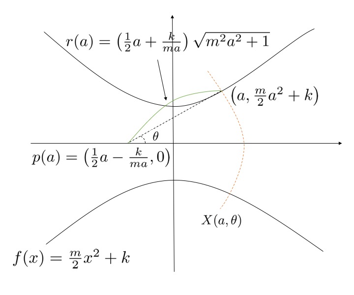
X⁡(a,θ)=(X1​(a,θ),X2​(a,θ))=p⁡(a)+r⁡(a)​(cos⁡θ,sin⁡θ),|θ|<arctan⁡(m​a),\displaystyle X(a,\theta)=(X_{1}(a,\theta),X_{2}(a,\theta))=p(a)+r(a)(\cos\theta,\sin\theta),\ \ \ |\theta|<\arctan(ma), (6.4)

where we choose p⁡(a)p(a), r⁡(a)r(a) so that the curve

Γ:={(X1​(a,θ),X2​(a,θ)):|θ|<arctan⁡(m​a)}∪{(−X1​(a,θ),X2​(a,θ)):|θ|<arctan⁡(m​a)}\Gamma:=\{(X_{1}(a,\theta),X_{2}(a,\theta))\,:\,|\theta|<\arctan(ma)\}\cup\{(-X_{1}(a,\theta),X_{2}(a,\theta))\,:\,|\theta|<\arctan(ma)\}

has a constant curvature, and is perpendicular to the boundary ∂Ω\partial\Omega. Indeed, set

p⁡(a):=(a2−km​a,0).p(a):=\left(\frac{a}{2}-\frac{k}{ma},0\right).

Then, we see that the tangent line for {(x1,x2)∣x2=f⁡(x1)}\{(x_{1},x_{2})\mid x_{2}=f(x_{1})\} at x1=ax_{1}=a goes through p⁡(a)p(a). Moreover, setting

r⁡(a):=|(a,m​a22+k)−p⁡(a)|=(a2+km​a)​m2​a2+1,r(a):=\left|\left(a,\frac{ma^{2}}{2}+k\right)-p(a)\right|=\left(\frac{a}{2}+\frac{k}{ma}\right)\sqrt{m^{2}a^{2}+1},

by elementary geometry, we can check that

Γ⊥∂Ω.\Gamma\bot\partial\Omega.

The parameter aa will be specified so that

c=1r⁡(a)c=\frac{1}{r(a)}

in Lemma 6.3.

Refer to caption
Refer to caption
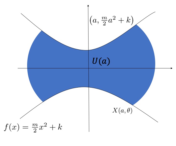
Fig. 2. Illustrations of (6.4) and (6.6)

The following definition is taken from [5, Definition 5.1.1].

Definition 6.2.

Let GG be a set in ℝn×J\mathbb{R}^{n}\times J, where JJ is an open interval in (0,T)(0,T). We say that GG is a set-theoretic subsolution (resp., supersolution) of

V=κ+con​ΓtwithΓt⊥∂ΩV=\kappa+c\quad\text{on}\ \Gamma_{t}\quad\text{with}\quad\Gamma_{t}\bot\partial\Omega (6.5)

if χG∗\chi_{G}^{\ast} is a viscosity subsolution (resp., (χG)∗(\chi_{G})_{\ast} is a viscosity supersolution) of (1.1)–(1.2) in ℝn×J\mathbb{R}^{n}\times J, where χG​(x,t)=1\chi_{G}(x,t)=1 if (x,t)∈G(x,t)\in G, and χG​(x,t)=0\chi_{G}(x,t)=0 if (x,t)∉G(x,t)\not\in G, and χG∗\chi_{G}^{\ast} and (χG)∗(\chi_{G})_{\ast} denote the upper semicontinuous envelope and the lower semicontinuous envelope of χG\chi_{G}, respectively. If GG is both a set-theoretic subsolution and supersolution of (6.5), GG is called a set-theoretic solution of (6.5).

Set

U(a):={(x1,x2)∈Ω:|x1|<X1(a,θ),|x2|<X2(a,θ),|θ|<arctan(ma)},\displaystyle U(a):=\{(x_{1},x_{2})\in\Omega:|x_{1}|<X_{1}(a,\theta),|x_{2}|<X_{2}(a,\theta),|\theta|<\arctan(ma)\}, (6.6)

and

rmin:=inf{r⁡(a):a>0}.r_{\min}:=\inf\{r(a):a>0\}. (6.7)

Then, rminr_{\min} is positive since rr is a continuous positive function in (0,∞)(0,\infty) and

lima→0r⁡(a)=lima→∞r⁡(a)=∞.\displaystyle\lim_{a\rightarrow 0}r(a)=\lim_{a\rightarrow\infty}r(a)=\infty. (6.8)

Moreover, by direct computation, we have

r′​(a)=1m2​a2+1​(m2​a2+12−km​a2).r^{\prime}(a)=\frac{1}{\sqrt{m^{2}a^{2}+1}}\left(m^{2}a^{2}+\frac{1}{2}-\frac{k}{ma^{2}}\right).

Therefore, rr has only one critical point a∗=12​m​−1+1+16​m​ka_{*}=\frac{1}{2m}\sqrt{-1+\sqrt{1+16mk}} in (0,∞)(0,\infty) and rmin=r⁡(a∗)r_{\min}=r(a_{*}). In addition,

r′​(a)<0r^{\prime}(a)<0 if a<a∗a<a_{*}, and r′​(a)>0r^{\prime}(a)>0 if a>a∗a>a_{*}. (6.9)
Lemma 6.3.

If c=1r⁡(a)c=\frac{1}{r(a)} for some a>0a>0, then U⁡(a)U(a) is a set-theoretic stationary solution of (1.1)–(1.2).

Proof.

As a consequence of the nice characterization of set-theoretic solutions in [5, Theorem 5.1.2], U⁡(a)U(a) is a set-theoretic stationary solution of (6.5) if and only if 0=κ+c0=\kappa+c on ∂U⁡(a)∩Ω\partial U(a)\cap\Omega and the right angle condition holds. The equality follows from the fact that ∂U⁡(a)∩Ω\partial U(a)\cap\Omega contains two arcs of two circles of the same radius r⁡(a)r(a) and curvature κ=−r​(a)−1=−c\kappa=-r(a)^{-1}=-c.

On the other hand, these arcs intersect with ∂Ω\partial\Omega at four points (a,±f⁡(a))(a,\pm f(a)), (−a,±f⁡(a))(-a,\pm f(a)). By symmetry, it suffices to prove the right angle condition at (a,f⁡(a))(a,f(a)). Notice that

(a,f⁡(a))=(X1​(a,arctan⁡(m​a)),X2​(a,arctan⁡(m​a)))=p⁡(a)+r⁡(a)m2​a2+1⋅(1,m​a).\displaystyle(a,f(a))=(X_{1}(a,\arctan(ma)),X_{2}(a,\arctan(ma)))=p(a)+\frac{r(a)}{\sqrt{m^{2}a^{2}+1}}\cdot(1,ma).

Therefore, the line joining (a,f⁡(a))(a,f(a)) and p⁡(a)p(a), the center of the arc, is tangent to ∂Ω\partial\Omega at (a,f⁡(a))(a,f(a)). Thus, ∂U⁡(a)∩Ω\partial U(a)\cap\Omega satisfies the right angle condition at (a,f⁡(a))(a,f(a)). ∎

Theorem 6.4.

If c∈(0,1rmin)c\in(0,\frac{1}{r_{\min}}), then there exist two positive constants a1<a2a_{1}<a_{2} such that U⁡(ai)U(a_{i}) is a set-theoretic stationary solution of (6.5) for i=1,2i=1,2.

Proof.

Thanks to (6.7)–(6.9), there exist two positive constants a1,a2a_{1},a_{2} with a1<a∗<a2a_{1}<a_{*}<a_{2} such that

r⁡(a1)=r⁡(a2)=1c.\displaystyle r(a_{1})=r(a_{2})=\frac{1}{c}. (6.10)

By Lemma 6.3, U⁡(ai)U(a_{i}) is a set-theoretic stationary solution of (6.5) for i=1,2i=1,2. ∎

6.2. Stability

Let aia_{i} be the constants given by Theorem 6.4 for i=1,2i=1,2. In this section, we prove that U⁡(a1)U(a_{1}) given by (6.6) is a set-theoretic solution which is stable in the sense of Theorem 6.1.

Lemma 6.5.

Let l1∈(0,a1)l_{1}\in(0,a_{1}), l2∈(0,a2−a1)l_{2}\in(0,a_{2}-a_{1}) and δ>0\delta>0. Set a¯​(t):=a1−l1​e−δ​t\underline{a}(t):=a_{1}-l_{1}e^{-\delta t} and a¯​(t):=a1+l2​e−δ​t\overline{a}(t):=a_{1}+l_{2}e^{-\delta t}. There exists δ0=δ0​(m,k,l1,l2)\delta_{0}=\delta_{0}(m,k,l_{1},l_{2}) such that U​(a¯​(t))U(\underline{a}(t)) and U​(a¯​(t))U(\overline{a}(t)) are a set-theoretic subsolution and supersolution to (6.5) for all δ∈(0,δ0)\delta\in(0,\delta_{0}), respectively.

Proof.

We only prove that U​(a¯​(t))U(\underline{a}(t)) is a set-theoretic subsolution, since we can similarly prove that U​(a¯​(t))U(\overline{a}(t)) is a set-theoretic supersolution. Let X~​(t):=X​(a¯​(t),θ)\tilde{X}(t):=X(\underline{a}(t),\theta). From the characterization of set-theoretic solutions in [5, Theorem 5.1.2], it suffices to show that for t⩾0t\geqslant 0,

d​X~d​t⋅𝐧→⩽−1r​(a¯​(t))+c for all ​t>0,\displaystyle\frac{d\tilde{X}}{dt}\cdot\vec{\mathbf{n}}\leqslant-\frac{1}{r(\underline{a}(t))}+c\quad\hbox{ for all }t>0, (6.11)

where 𝐧→\vec{\mathbf{n}} is the outward normal vector 𝐧→\vec{\mathbf{n}} of U​(a¯​(t))U(\underline{a}(t)), that is, 𝐧→=(cos⁡θ,sin⁡θ)\vec{\mathbf{n}}=(\cos\theta,\sin\theta).

Note that

d​X~d​t⋅𝐧→=∂a¯∂t​∂X∂a⋅𝐧→=δ​l1​e−δ​t​∂X∂a⋅𝐧→=δ⁡(a1−a¯​(t))​∂X∂a⋅𝐧→.\frac{d\tilde{X}}{dt}\cdot\vec{\mathbf{n}}=\frac{\partial\underline{a}}{\partial t}\frac{\partial{X}}{\partial a}\cdot\vec{\mathbf{n}}=\delta l_{1}e^{-\delta t}\frac{\partial{X}}{\partial a}\cdot\vec{\mathbf{n}}=\delta(a_{1}-\underline{a}(t))\frac{\partial{X}}{\partial a}\cdot\vec{\mathbf{n}}.

Also, for any constant L>0L>0, there exists C=C⁡(m,k,L)>0C=C(m,k,L)>0 such that

∂X∂a​(a,θ)⋅𝐧→=p′​(a)⋅𝐧→+r′​(a)≤|p′​(a)|+r′​(a)\displaystyle\frac{\partial{X}}{\partial a}(a,\theta)\cdot\vec{\mathbf{n}}=p^{\prime}(a)\cdot\vec{\mathbf{n}}+r^{\prime}(a)\leq|p^{\prime}(a)|+r^{\prime}(a)
=\displaystyle= 12+m2​a2+12m2​a2+1+m​km2​a2+1+m2​a2+1≤C\displaystyle\,\frac{1}{2}+\frac{m^{2}a^{2}+\frac{1}{2}}{\sqrt{m^{2}a^{2}+1}}+\frac{mk}{m^{2}a^{2}+1+\sqrt{m^{2}a^{2}+1}}\leq C

for all a∈(0,L)a\in(0,L) and θ∈(−π2,π2)\theta\in(-\frac{\pi}{2},\frac{\pi}{2}). Therefore,

d​X~d​t⋅𝐧→=δ⁡(a1−a¯​(t))​∂X∂a⋅𝐧→⩽C​δ​(a1−a¯​(t)).\displaystyle\frac{d\tilde{X}}{dt}\cdot\vec{\mathbf{n}}=\delta(a_{1}-\underline{a}(t))\frac{\partial{X}}{\partial a}\cdot\vec{\mathbf{n}}\leqslant C\delta(a_{1}-\underline{a}(t)).

The observation (6.9) implies that r⁡(a¯​(t))>r⁡(a1)=c−1r(\underline{a}(t))>r(a_{1})=c^{-1} for all t⩾0t\geqslant 0, and thus we get

(d​X~d​t⋅𝐧→)​(−1r​(a¯​(t))+c)−1⩽δ​C​a1−a¯​(t)1r⁡(a1)−1r​(a¯​(t)).\displaystyle\left(\frac{d\tilde{X}}{dt}\cdot\vec{\mathbf{n}}\right)\left(-\frac{1}{r(\underline{a}(t))}+c\right)^{-1}\leqslant\delta C\frac{a_{1}-\underline{a}(t)}{\frac{1}{r(a_{1})}-\frac{1}{r(\underline{a}(t))}}.

Thus, (6.11) holds for δ∈(0,δ0)\delta\in(0,\delta_{0}), where

δ0:=(C​supa∈[a1−l1,a1+l2]h⁡(a))−1.\displaystyle\delta_{0}:=\left(C\sup_{a\in[a_{1}-l_{1},a_{1}+l_{2}]}h(a)\right)^{-1}.

Here the function h:[a1−l1,a1+l2]→ℝh:[a_{1}-l_{1},a_{1}+l_{2}]\rightarrow\mathbb{R} is given by

h⁡(a):={a1−a1r⁡(a1)−1r⁡(a) for ​a∈[a1−l1,a1+l2]∖{a1},−r2​(a1)r′​(a1) for ​a=a1.h(a):=\begin{cases}\dfrac{a_{1}-a}{\frac{1}{r(a_{1})}-\frac{1}{r(a)}}\quad&\hbox{ for }a\in[a_{1}-l_{1},a_{1}+l_{2}]\setminus\{a_{1}\},\\ \\ \dfrac{-r^{2}(a_{1})}{r^{\prime}(a_{1})}\quad&\hbox{ for }a=a_{1}.\end{cases}

Since a1+l2<a2a_{1}+l_{2}<a_{2}, by (6.9) we have r⁡(a)≠r⁡(a1)r(a)\neq r(a_{1}) in [a1−l1,a1+l2]∖{a1}[a_{1}-l_{1},a_{1}+l_{2}]\setminus\{a_{1}\} and r′​(a1)<0r^{\prime}(a_{1})<0. Therefore, hh is well-defined and continuous in [a1−l1,a1+l2][a_{1}-l_{1},a_{1}+l_{2}]. Thus, hh is bounded in [a1−l1,a1+l2][a_{1}-l_{1},a_{1}+l_{2}], and hence, δ0>0\delta_{0}>0 is well-defined, which implies that (6.11) holds for all δ∈(0,δ0)\delta\in(0,\delta_{0}). ∎

Proof of Theorem 6.1.

We let α=0\alpha=0 and β=1\beta=1 for simplicity. Set

u¯​(x,t):=χU​(a¯​(t))¯​(x) and u¯​(x,t):=χU​(a¯​(t))​(x)\displaystyle\underline{u}(x,t):=\chi_{\overline{U(\underline{a}(t))}}(x)\quad\hbox{ and }\quad\overline{u}(x,t):=\chi_{U(\overline{a}(t))}(x)

for (x,t)∈Ω¯×[0,∞)(x,t)\in\overline{\Omega}\times[0,\infty), where a¯\underline{a} and a¯\overline{a} are the functions defined in Lemma 6.5. By Lemma 6.5, we see that u¯\underline{u} and u¯\overline{u} are a subsolution and a supersolution of (1.1)–(1.2), respectively. Due to (6.3), we get

u¯​(⋅,0)=χU​(a¯​(0))¯⩽u0⩽χU​(a¯​(0))=u¯​(⋅,0)​ on ​Ω¯.\displaystyle\underline{u}(\cdot,0)=\chi_{\overline{U(\underline{a}(0))}}\leqslant u_{0}\leqslant\chi_{U(\overline{a}(0))}=\overline{u}(\cdot,0)\hbox{ on }\overline{\Omega}.

In addition, since

U⁡(a)⊂V⁡(a):=[−(|p⁡(a)|+r⁡(a)),|p⁡(a)|+r⁡(a)]×[−f⁡(a),f⁡(a)]U(a)\subset V(a):=[-(|p(a)|+r(a)),|p(a)|+r(a)]\times[-f(a),f(a)]

by construction for p⁡(a)p(a) and r⁡(a)r(a) given in (6.4) and f⁡(a)=m2​a2+kf(a)=\frac{m}{2}a^{2}+k, we obtain

supp⁡(u¯)⊂⋃a∈[a1−l1,a1]V⁡(a)×[0,∞)​ and ​supp⁡(u¯)⊂⋃a∈[a1,a1+l2]V⁡(a)×[0,∞).\displaystyle\operatorname{supp}(\underline{u})\subset\bigcup_{a\in[a_{1}-l_{1},a_{1}]}V(a)\times[0,\infty)\hbox{ and }\operatorname{supp}(\overline{u})\subset\bigcup_{a\in[a_{1},a_{1}+l_{2}]}V(a)\times[0,\infty).

As |p⁡(⋅)|+r⁡(⋅)|p(\cdot)|+r(\cdot) and ff are continuous on [a1−l1,a1+l2][a_{1}-l_{1},a_{1}+l_{2}], there exists a constant R0>0R_{0}>0 satisfying (6.2).

By the comparison principle for (1.1)–(1.3), Proposition 2.2, we get

u¯​(⋅,t)⩽u⁡(⋅,t)⩽u¯​(⋅,t)on​Ω¯for all​t>0.\displaystyle\underline{u}(\cdot,t)\leqslant u(\cdot,t)\leqslant\overline{u}(\cdot,t)\quad\text{on}\ \overline{\Omega}\quad\text{for all}\ t>0.

On the other hand, since both a1−l1​e−δ​ta_{1}-l_{1}e^{-\delta t} and a1+l2​e−δ​ta_{1}+l_{2}e^{-\delta t} converge to a1a_{1} as tt goes to infinity,

limt→∞u¯​(x,t)=limt→∞u¯​(x,t)=1 for ​x∈U⁡(a1),\displaystyle\lim_{t\rightarrow\infty}\underline{u}(x,t)=\lim_{t\rightarrow\infty}\overline{u}(x,t)=1\quad\hbox{ for }x\in U(a_{1}),

and

limt→∞u¯​(x,t)=limt→∞u¯​(x,t)=0 for ​x∈Ω¯∖U⁡(a1)¯,\displaystyle\lim_{t\rightarrow\infty}\underline{u}(x,t)=\lim_{t\rightarrow\infty}\overline{u}(x,t)=0\quad\hbox{ for }x\in\overline{\Omega}\setminus\overline{U(a_{1})},

which finish the proof. ∎

Acknowledgements

The authors are extremely grateful to the anonymous referee for his/her careful reading and very constructive comments, which help much to improve the presentation of the paper.

References

  • [1] S. Aimi. Level set mean curvature flow with Neumann boundary conditions. arXiv preprint arXiv:2103.16386. 2021.
  • [2] Y. G. Chen, Y. Giga, and S. Goto. Uniqueness and existence of viscosity solutions of generalized mean curvature flow equations. J. Differential Geom. 33 (1991), no. 3, 749–786.
  • [3] A. Cesaroni, and M. Novaga. Long-time behavior of the mean curvature flow with periodic forcing. Comm. Partial Differential Equations, 38 (2013), no. 5, 780–801.
  • [4] L. C. Evans, and J. Spruck. Motion of level sets by mean curvature. I. J. Differential Geom. , 33 (1991), no. 3, 635–681.
  • [5] Y. Giga. Surface evolution equations-A level set approach, Monographs in Mathematics, Birkhäuser, 2006.
  • [6] Y. Giga, H. Mitake, T. Ohtsuka, and Hung V. Tran. Existence of asymptotic speed of solutions to birth and spread type nonlinear partial differential equations. Indiana Univ. Math. J., 70 (2021), no. 1, 121–156.
  • [7] Y. Giga, H. Mitake, and H. V. Tran. Remarks on large time behavior of level-set mean curvature flow equations with driving and source terms. Discrete Contin. Dyn. Syst. Ser. B, 25 (2020), no. 10, 3983–3999.
  • [8] Y. Giga, H. Mitake, and H. V. Tran. On asymptotic speed of solutions to level-set mean curvature flow equations with driving and source terms. SIAM J. Math. Anal., 48 (2016), no. 5, 3515–3546.
  • [9] Y. Giga, M. Ohnuma, and M.-H. Sato. On the strong maximum principle and the large time behavior of generalized mean curvature flow with the Neumann boundary condition. J. Differential Equations, 154 (1999), no. 1, 107–131.
  • [10] Y. Giga, and M.-H. Sato. Generalized interface evolution with the Neumann boundary condition. Proc. Japan Acad. Ser. A Math. Sci., 67 (1991), no. 8, 263–266.
  • [11] Y. Giga, and M.-H. Sato. Neumann problem for singular degenerate parabolic equations. Differential and Integral Equations, 6 (1993), no. 6, 1217–1230.
  • [12] Y. Giga, Hung V. Tran, and L. Zhang. On obstacle problem for mean curvature flow with driving force. Geom. Flows, 4 (2019), no. 1, 9–29.
  • [13] B. Guan. Mean curvature motion of nonparametric hypersurfaces with contact angle condition. Elliptic and parabolic methods in geometry, 47–56, 1996.
  • [14] N. Hamamuki, and K. Misu. Asymptotic shape of solutions to the mean curvature flow equation with discontinuous source terms, in preparation.
  • [15] G. Huisken. Nonparametric mean curvature evolution with boundary conditions. J. Differential Equations 77 (1989), no. 2, 369–378.
  • [16] H. Ishii. Weak KAM aspects of convex Hamilton-Jacobi equations with Neumann type boundary conditions. J. Math. Pures Appl. (9) 95 (2011), no. 1, 99–135.
  • [17] I. Kim, and D. Kwon. Volume preserving mean curvature flow for star-shaped sets. Calc. Var. Partial Differential Equations, 59 (2020), no. 2, Paper No. 81, 40 pp.
  • [18] I. Kim, D. Kwon, and N. Požár. On volume-preserving crystalline mean curvature flow. arXiv preprint arXiv:2012.13839. 2020.
  • [19] P.-L. Lions, P. E. Souganidis. Homogenization of degenerate second-order PDE in periodic and almost periodic environments and applications. Ann. Inst. H. Poincaré Anal. Non Lineairé 22 (2005), no. 5, 667–677.
  • [20] X.-N. Ma, P.-H. Wang, W. Wei. Constant mean curvature surfaces and mean curvature flow with non-zero Neumann boundary conditions on strictly convex domains. J. Funct. Anal. 274 (2018), no. 1, 252–277.
  • [21] H. Matano, K.-I. Nakamura, B. Lou. Periodic traveling waves in a two-dimensional cylinder with saw-toothed boundary and their homogenization limit, Netw. Heterog. Media 1 (2006), no. 4, 537–568.
  • [22] M. Mizuno, and K. Takasao. Gradient estimates for mean curvature flow with Neumann boundary conditions. NoDEA Nonlinear Differential Equations Appl. , 24 (2017), no. 4, Paper No. 32, 24 pp.
  • [23] T. Ohtsuka. Discontinuous stationary solution to generalized eikonal-curvature equation and its stability. Comment. Math. Univ. St. Pauli 63 (2014), no. 1-2, 233–260.
  • [24] J. Xu. Mean curvature flow of graphs with Neumann boundary conditions. Manuscripta Math, 158 (2019), no. 1-2, 75–84.