Rectangles conformally inscribed in linesThanks: August 11, 2026
Abstract.
A parallelogram is conformally inscribed in four lines in the plane if it is inscribed in a scaled copy of the configuration of four lines. We describe the geometry of the three-dimensional Euclidean space whose points are the parallelograms conformally inscribed in sequence in these four lines. In doing so, we describe the flow of inscribed rectangles by introducing a compact model of the rectangle inscription problem.
1991 Mathematics Subject Classification
Primary 52C30, 51N10, 51N151. Introduction
This article continues recent work from [6, 7, 8, 9, 10], in which the geometric and algebraic properties of rectangles inscribed in lines in the plane are studied. Describing such rectangles is the key step to describing rectangles inscribed in polygons, which in turn is related to the rectangle peg problem of finding rectangles inscribed in simple closed curves; see for example [2, 3, 5, 4, 9]. To describe rectangles inscribed in lines, we need only consider four lines at a time. Denote by a configuration consisting of two pairs of lines and , where not all four lines are parallel. A rectangle is inscribed in if its vertices lie on in either clockwise or counterclockwise order. Each rectangle inscribed in lies on a path of inscribed rectangles, either a “slope path” parametrized by the slope of the rectangles or an “aspect path” parametrized by aspect ratio [7, 8]. (The images of these two paths can coincide, as they do in Figure 1.) As they travel either path, the rectangles eventually grow without bound, yet as they do so their slopes and aspect ratios converge to a pair of numbers that do not occur as the slope or aspect ratio of any rectangle inscribed in .

These two numbers, a missing slope and a missing aspect ratio, suggest a missing rectangle, a rectangle inscribed at infinity. In [7, Section 3], this is dealt with by viewing the inscribed rectangles as points in , with two coordinates for each vertex of the rectangle. Taking the projective closure of the set of inscribed rectangles in finds the missing rectangle as a point at infinity. The vertices of a rectangle can be read off from the coordinates of this rectangle at infinity, but instead of a rectangle inscribed in the four lines, it is an equivalence class of rectangles inscribed in the configuration viewed from infinity, in which all four lines go through the same point.
It is proved in [7, Theorem 3.2] that when viewed as points in , the rectangles inscribed in constitute a line or a planar hyperbola in , which if the rectangles at infinity are included becomes either a simple closed curve of rectangles in the projective closure of or a pair of lines. This insertion of a missing rectangle at infinity is sufficient for the purposes in [7], but with this approach part of the geometry of the rectangle inscription problem breaks at infinity, since at infinity, and only at infinity, the configuration switches from to the configuration in which all four lines are translated to the origin. Also, the rectangle at infinity remains indefinite since it is really an equivalence class of rectangles rather a single rectangle through which the other inscribed rectangles pass.
These last two observations are the starting point of this article and suggest the need for a kind of curve selection lemma which chooses from each equivalence class in a rectangle in such a way that the set of selected rectangles is a simple closed curve of rectangles inscribed not only in but in scaled copies of also. Viewing as lines through the origin in , this can be accomplished using the fact that the 8-dimensional unit sphere is a double cover of . The desired simple closed curve of rectangles is then found on the unit sphere.
However, it’s possible to describe the data that determines the rectangles much more efficiently than as points in and to give a less generic explanation for the existence of a simple closed curve of rectangles that scale to the rectangles inscribed in . To do so, in Section 2 we define a notion of conformally inscribed parallelograms as those parallelograms that are inscribed in scaled copies of , and we show that the set of all such parallelograms inscribed in forms a three-dimensional Euclidean space with inner product determined by the diagonals of the parallelograms. This space has an orthonormal basis of three canonically chosen parallelograms that determine principal axes for . This is helpful because the equations that govern the inscribed rectangles are long and unwieldy, but they become simple and easy to work with in the coordinates induced by this orthonormal basis. The previous complexity of the equations is hidden in the coordinates for the parallelograms in the orthonormal basis.
Among the conformally inscribed rectangles are the unit rectangles, those conformally inscribed rectangles that have norm with respect to the inner product of . Every rectangle inscribed in the four lines can be represented by a unit rectangle inscribed in a scaled copy of the configuration of the four lines. We show that in the space of conformally inscribed parallelograms, the unit rectangles lie on an intersection of two cylinders and thus form an algebraic space curve. This curve is the union of two simple closed analytic curves, and each of these curves gives a compact solution to the rectangle inscription problem in the sense that these rectangles comprise a flow that after projection accounts for all rectangles inscribed in as well as those at infinity.
All this can be made more concrete by reinterpreting a model for the rectangle inscription problem from [6], where it is shown that locating the centers of the rectangles inscribed in is equivalent to describing the intersection of two hyperbolically rotated cones in . In the model, which we call in Section 7 the cone model for , the intersection of the two cones is a space curve that projects orthographically to a curve in consisting of the rectangle centers. This model also omits the rectangles at infinity: the space curve heads to infinity as the centers of the rectangles in the plane head to infinity.
However, as we discuss in Section 7, we may view the cone model as a chart in the three-dimensional projective space . If we exchange the plane in the cone model in which the cone apexes reside with the plane at infinity, we bring the missing rectangles at infinity into view. The hyperbolically rotated cones now have apex at infinity in this new model, which we call in Section 6 the cylinder model, and so become elliptical cylinders. The intersection of these two cylinders is a compact space curve which consists of the centers of the unit rectangles. The parallelograms at infinity lie in a plane in the cylinder model, and so having the flow of inscribed rectangles pass through a rectangle at infinity is simply a matter of having these rectangles pass through this plane. What makes this possible is a scaling dimension so that passing through the rectangles at infinity amounts to passing from positively scaled copies of to negatively scaled copies. It is this last feature, having another side of infinity, that is missing from the cone model for and which makes possible the approach taken in this article.
We have use MapleTM to assist with calculations and graphics.
2. Conformally inscribed parallelograms
When dealing with parallelograms inscribed in lines in the plane, we may reduce to the case of four lines. If the four lines are not all parallel, we can relabel and rotate the lines in order to reduce further to the following standing assumption for the article. (See [7, 9] for discussion of this reduction.) The restriction that the line go through the point can always be achieved by scaling the configuration .
Standing assumption. Throughout this article we work with two pairs of lines and in the real plane such that the four lines do not meet in a single point; goes through the point ; and and meet in the origin and only in the origin. The configuration consisting of the two pairs of lines and is denoted .
We work with equations for these four lines, and for this we use the following notation.
Notation 2.1.
We denote by the real numbers for which the equations defining the lines are
We write for , for , etc..
Notation 2.2.
Let . For a line defined by an equation of the from , we denote by the line in defined by . With the lines from the standing assumption, the line is defined by and the line by . Since and pass through the origin, and . We denote by the resulting configuration consisting of the pairs and . Thus for , is a scaled copy of . The special case where is the configuration of the four lines through the origin. This is the configuration viewed from infinity.
Definition 2.3.
A parallelogram is inscribed in if the vertices of lie in sequence, either clockwise or counterclockwise, on the lines . Among inscribed parallelograms, we include the degenerate ones also, those whose sides all lie on the same line, or even whose sides consist of a single point, namely the origin in the configuration . A parallelogram in the plane is conformally inscribed in if can be inscribed in for some . In this case, we say is the scale of . If , then is inscribed at infinity for . We denote by the set of parallelograms conformally inscribed in .
We give the set of conformally inscribed parallelograms the structure of a Euclidean space. Define the sum of two parallelograms to be the parallelogram that results from adding vertices coordinatewise. If one of the parallelograms is inscribed in the configuration and the other in , then the sum of the two parallelograms is inscribed in the configuration . Similarly, if , then multiplying the coordinates of each vertex of a parallelogram inscribed in by results in a parallelogram inscribed in . The degenerate parallelogram all of whose vertices are the origin is the additive identity for . With these operations, is a vector space.
We define an inner product on in terms of the diagonals of the parallelograms in . It is convenient to view these diagonals as vectors, as in the next definition.
Definition 2.4.
Let be a parallelogram in , and let be the scale of . Denote by , , the vertices of . The and diagonal vectors of are, respectively,
The side vectors of are and .
Definition 2.5.
We define an inner product on for each by
and we denote by the norm induced by this inner product, i.e.
An argument similar to that for the parallelogram law shows that the second equality in the definition holds. Thus is the sum of the squared lengths of the diagonals of , which in turn is twice the sum of the squared lengths of the sides of . That the bilinear map defines an inner product follows from the fact that if , then , which can only happen if is the degenerate parallelogram that is simply the origin in . Thus if and only if is the zero element in .
Theorem 2.6.
With the inner product in Definition 2.5, is a Euclidean space having an orthonormal basis of such that and are degenerate parallelograms and and See Figure . The parallelograms and are at infinity if and only if at least one of the pairs or consists of parallel lines.

Proof.
We first show Let . By [7, Lemma 4.3], a quadrilateral inscribed in with vertices , , is a parallelogram if and only if and (By our standing assumptions, , so this is a simple consequence of the fact that a quadrilateral is a parallelogram if and only if the midpoints of its two diagonals coincide.) Since a parallelogram is specified by its vertices, each choice of determines a unique parallelogram in according to these equations, and every parallelogram in can be specified by the choice of . Thus .
Next, observe that if and are parallelograms in such that and are the zero vector, then and are orthogonal: . Thus, if and are parallelograms such that the diagonal of and the diagonal of have length , then and are orthogonal.
We construct the parallelogram first. If neither pair or consists of parallel lines, set
Then, using the expressions above involving and , these choices for define a parallelogram in with vertices , for . Also, a calculation shows and , so that defines a parallelogram in whose diagonal vector is . Since does not go through the origin, the diagonal vector of is not . Multiplying by , we obtain a parallelogram in with norm 1 whose diagonal has length .
On the other hand, if and are parallel or and are parallel, then with
we obtain a parallelogram with and , and this parallelogram can be rescaled to a parallelogram that has norm .
Next, to define , assume first that neither pair or is parallel. Set
As above, this defines a parallelogram with vertices , . A calculation shows and . Since the lines do not all go through the origin, it cannot be that and . Thus , and as above, rescaling gives a parallelogram with norm 1 whose diagonal has length .
On the other hand, if , then the values define a parallelogram that after rescaling gives the parallelogram . If instead and , then
defines a parallelogram that after rescaling gives .
The construction of and shows that one of the parallelograms is at infinity (i.e., has scale ) if and only if both are; if and only if at least one of the pairs and consists of parallel lines. Also, since and , the parallelograms and are orthogonal.
Finally, since has dimension , the orthogonal complement of the subspace of spanned by and has dimension . Choose a parallelogram in this subspace for which . Since is the zero vector and is orthogonal to , it follows that . Similarly, . ∎
Remark 2.7.
Suppose neither pair or consists of parallel lines. The construction of the parallelogram in the proof of Theorem 2.6 leads to the following method for finding . Let be the median curve for the lines and along a line perpendicular to the degenerate parallelogram ; that is, let be the line consisting of the midpoints of the line segments that join and and are perpendicular to the degenerate parallelogram . Similarly, let be the line of midpoints of the segments perpendicular to that join and . If and intersect at a point then this point is the center of the copy of scaled to a parallelogram inscribed in . This is illustrated in Figure 2. Otherwise, if and are parallel (see Figure 3), then is at infinity.
In light of the theorem, we introduce coordinates for the Euclidean space in terms of the basis .
Notation 2.8.
For , we denote by the parallelogram in . We also denote by the scales of the parallelograms .
Since is an orthonormal basis, for each , we have
Thus in the coordinates , the set of unit parallelograms in , i.e., those with norm , is a sphere defined by .
By Theorem 2.6, one of the parallelograms is at infinity if and only if both are; if and only if at least one of the pairs and consists of parallel lines. In this case, the parallelogram is not at infinity since otherwise the linearly independent vectors all lie in the two-dimensional subspace of consisting of the parallelograms at infinity, a contradiction. On the other hand, if and are not at infinity (and so neither pair of lines or consists of parallel lines), then the orthogonal complements and of and are distinct planes through the origin. These two planes meet in a line which contains . This line, and hence , can be at infinity or not. See Figure 3 for an example where is at infinity.

The parallelograms inscribed in can be distinguished among the parallelograms conformally inscribed in , according to the next corollary. Recall that are the scales of , respectively.
Corollary 2.9.
For each , the set of parallelograms inscribed in is a plane in defined by . This plane goes through the origin if and only if , and so the parallelograms at infinity form a two-dimensional subspace of .
Proof.
For each , the parallelograms inscribed in are the parallelograms that have scale . If and are two parallelograms in of scales and , then the scale of is since and imply . Thus the scale of the parallelogram is The plane in defined by this equation goes through the origin if and only if . The parallelograms of scale are precisely the parallelograms at infinity, so the corollary follows. ∎
Since is a vector space, we may consider its projective space whose points are the lines in through the origin. The next corollary is a straightforward consequence of the fact from Theorem 2.6 that is a three-dimensional vector space.
Corollary 2.10.
The projective space of is the projective closure of the plane of parallelograms in that are inscribed in . Each point in is the set of all the scaled copies of a parallelogram inscribed in or a parallelogram at infinity for . ∎
The next theorem shows that the inner product on is a natural choice, being induced as it by the usual dot product on . This dot product involves the diagonal vectors of the parallelogram, which when extracted from a parallelogram in results in the loss of the location of the parallelograms since only the shape and orientation is preserved by the diagonal vectors. Thus, on their own, the diagonal vectors determine only up to translation. However, with the data of the original configuration in which was conformally inscribed, we can recover the location of . In particular, there is only one parallelogram in that has a given set of diagonal vectors. Similarly, there is only one parallelogram in that has a given set of side vectors.
Theorem 2.11.
The linear transformation that sends a parallelogram in to its diagonal vectors in is an isometry onto its image. Thus the diagonal vectors of uniquely determine , as do the side vectors.
Proof.
Let be the matrix
Since is an orthonormal basis, this matrix has rank . If is a parallelogram with coordinates and vertices , for , then since , we have
Since has rank , is the unique solution to this matrix equation. The matrix is the representation with respect to the basis of the linear transformation that sends a parallelogram to its diagonal vectors, and so this transformation is injective. The transformation is an isometry onto its image since and the latter expression is an application of the standard norm for .
To prove the statement about side vectors, observe that and . Thus, with the identity matrix, we have
This gives an invertible linear transformation from the space of diagonal vectors to the space of side vectors, and since the representation of by its diagonal vectors is unique, so is the representation of by its side vectors. ∎
3. The geometry of the space of parallelograms
In this section we describe the geometry of the set of rectangles in the Euclidean space . Since contains not only the rectangles inscribed in but also those conformally inscribed in , there is flexibility in choosing rectangles to represent, up to scale, the rectangles inscribed in . A natural way to do this is to select the unit rectangles, those rectangles having norm in , and we do this in this section.
The parallelograms from Theorem 2.6, along with the coordinates that represent the parallelograms in , play a main role in our approach in this section. The three lines in that pass through the origin and each of these three parallelograms form orthogonal axes for and make the geometric properties of the set of unit rectangles a straightforward matter. For example, these axes and the invariants of introduced in the following notation are all that are needed to specify the unit rectangles, as we show in Theorem 3.4.
Notation 3.1.
With the parallelogram given by Theorem 2.6, let be the squared length of the diagonal of , and be the squared length of the diagonal; that is,
and .
Since , we have .
It is possible that or . For example, if or and are parallel and the intersection of and is equidistant from lines and . See Figure 4 for the latter example.
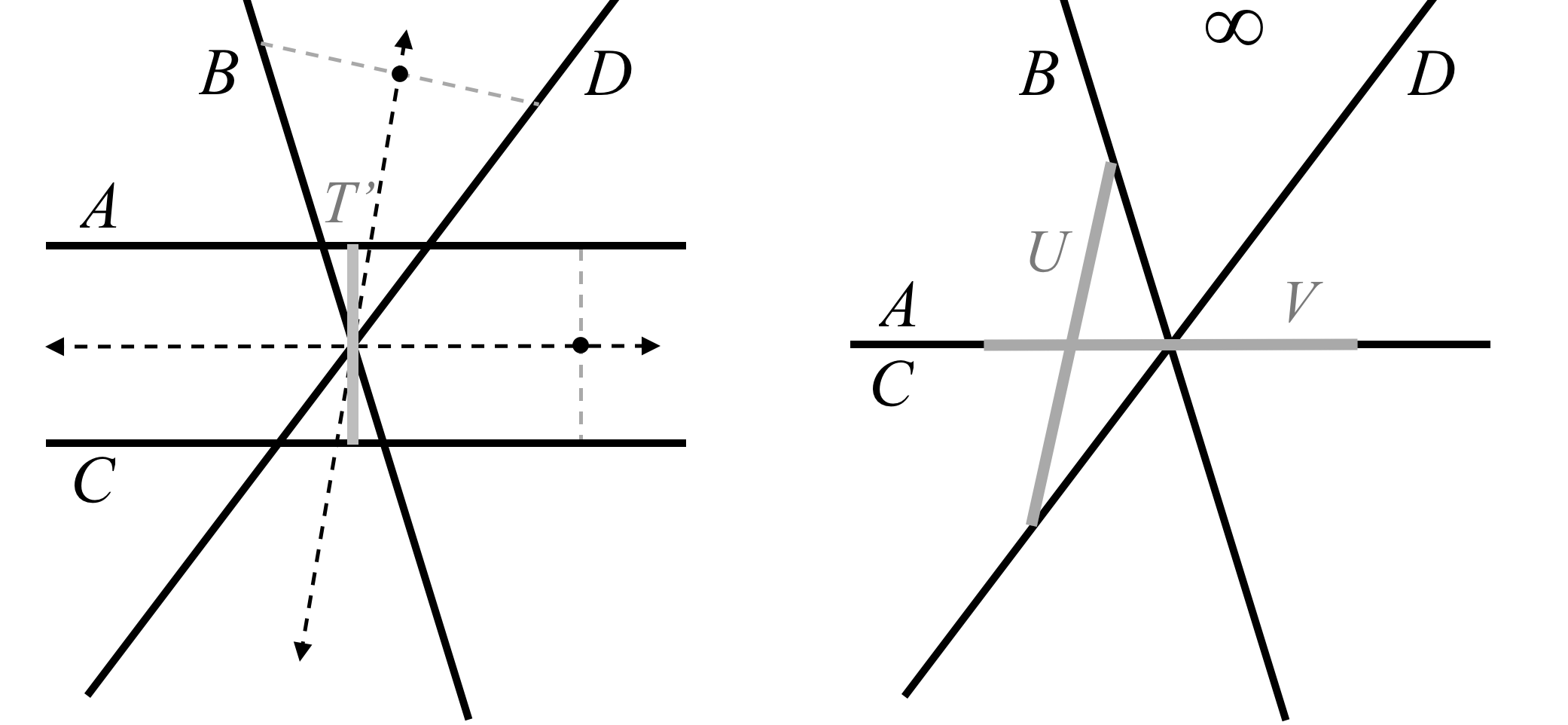
Lemma 3.2.
In the coordinates , the set of unit rectangles in is an algebraic curve given by the intersection of the surfaces defined by
and
Each of these surfaces is an elliptical cylinder or pair of parallel planes see Figure . The first surface is the set of parallelograms in whose diagonal has length and the second is the set of parallelograms whose diagonal has length .
Proof.
First we show that for a parallelogram in with coordinates ,
and .
Since and , we have . Therefore, since and , Theorem 2.6 implies
This shows the equation defines the set of parallelograms whose diagonal has squared length . A similar argument shows and hence defines the set of parallelograms whose diagonal has squared length . The parallelograms that lie in this intersection of these two quadrics have diagonals of squared length , and so these parallelograms are precisely the unit rectangles in .
Finally, if and , the equations and define two elliptical cylinders that meet on the unit sphere in . Otherwise, if , then defines a pair of parallel planes in and similarly for and the second surface. ∎

The cylinders in Theorem 3.2 are identical up to rotation if and only , if and only if the parallelogram is a rectangle. As we show in the next theorem, this condition is significant for the geometry of the set of rectangles inscribed in the configuration because it coincides with a degeneracy condition for . To define what is meant by “degenerate” here, we recall how in [7, Definition 2.2] a pair of diagonals and are defined for the configuration . (These diagonals are lines in rather that line segments.)
If , then the diagonal of is the line in through the origin () and , which is possibly at infinity. Otherwise, if , then is the line through the origin that is orthogonal to .
If , then the diagonal is the line in through and . Otherwise, if , then is the line through that is orthogonal to .
Definition 3.3.
The configuration is degenerate if the diagonals of are perpendicular.
(We are assuming here the convention that the line at infinity for the projective closure of is perpendicular to every line in .)
The rectangle locus for , which is discussed again in Section 6, is the set of centers of the rectangles inscribed in . The motivation for the terminology of degeneracy in Definition 3.3 is that if neither pair or consists of parallel lines, then is degenerate if and only if the rectangle locus is a degenerate hyperbola with one of the two lines that comprise the hyperbola possibly at infinity [7, Section 9]. More generally, regardless of whether or consist of parallel lines, the set of rectangles inscribed in may be viewed as a subspace of , with each vertex occupying two coordinates in . In this space, is degenerate if and only if the set of rectangles is a pair of intersection lines in [7, Theorem 7.1]. Theorem 3.4 shows how degeneracy is reflected in the set of rectangles in .
Theorem 3.4.
In the coordinates , the set of rectangles in is defined by the equation This set is a pair of planes defined by if and only if the parallelogram from Theorem 2.6 is a rectangle, if and only if is degenerate. Otherwise, the set of rectangles is an elliptical cone whose central axis is either the axis or the axis and whose apex is at the origin.
Proof.
By Lemma 3.2, the set of unit rectangles is the intersection of and . Let be a rectangle in with coordinates . If (in which case is the degenerate rectangle consisting of a single point, the origin), then . Otherwise, suppose not all of are zero, so that is not zero. Then is a unit rectangle and so and , from which we conclude .
Conversely, if is a parallelogram for which , then with , we have if that , and hence is a degenerate rectangle, while if , then is by Lemma 3.2 a unit rectangle, and so is a rectangle, which proves the set of rectangles in is defined by the equation . If , this equation defines an elliptical cone whose central axis is either the -axis or -axis and whose apex is at the origin.
Now suppose is a rectangle. By Lemma 3.2, , and so the set of rectangles is defined by and hence is the pair of planes defined by . By Corollary 2.9, the set of parallelograms inscribed in is a plane in that does not go through the origin. Therefore, this plane intersects the pair of planes defined by in a pair of lines, and so is degenerate by [7, Theorem 7.1]. Conversely, if is degenerate, this same reference implies the plane of parallelograms inscribed in intersects the surface defined by in a pair of lines. Since a plane intersects an elliptical cone in a pair of lines if and only if the plane goes through the apex, this implies the surface defined by is not an elliptical cone, and thus . Therefore, is a rectangle. ∎
4. Conformal solutions
By Lemma 3.2, the set of unit rectangles is an algebraic curve in , a bicylindrical curve, that lies on the unit sphere in . In this section we show the set of unit rectangles is a union of two simple closed analytic curves, either one of which can be taken as a conformal solution for in the following sense.
Definition 4.1.
A conformal solution for is a set of rectangles in such that each rectangle inscribed in and at infinity for is scaled from a rectangle in , and for all but at most one such rectangle , there is a unique rectangle in that scales to .
Thus a conformal solution is a solution for the rectangle inscription problem up to scale that includes also rectangles at infinity. The last condition that permits two rectangles in to scale to the same inscribed rectangle for at most one choice of is needed when dealing with a singularity that occurs in the degenerate case. This is explained by Corollary 4.4.
The symmetry of the set of unit rectangles about the origin implies that if is a conformal solution for , so is . With the coordinates , finding a conformal solution is a straightforward matter of parametrization, as we show in the proof of the next theorem.
Theorem 4.2.
There is a simple closed analytic curve in such that is a conformal solution for and is the set of unit rectangles in see Figure .
Proof.
By Lemma 3.2, the set of unit rectangles is the intersection of the surfaces defined by and . We consider two cases in order to define .
Suppose first . Since , this implies . At the end of the proof we explain the modification needed if . A parallelogram in with coordinates is on the intersection of these two quadrics if and only if and ; if and only if
Since we have . Substituting , we obtain that the intersection of the two quadrics is the set of parallelograms with coordinates
Define
Since , is defined and analytic on all of . Using the fact that and , it follows that the intersection of the two quadrics (which is the set of unit rectangles) is the union of the image of and the image of . The maps and define simple closed analytic curves Image() and Image() on the unit sphere, and the union of these two curves is the set of unit rectangles.
Still in the case , to see that each rectangle inscribed in or at infinity is scaled from a rectangle in , let be a rectangle in that is either inscribed in or at infinity. Then the coordinates of are not all zero. Let . Now is in the image of if and only if , while is in the image of if and only if . If , then gives the coordinates of a unit rectangle in the image of such that . Otherwise, if , then gives the coordinates of a unit rectangle in the image of such that . A similar argument shows that each rectangle inscribed in or at infinity is scaled from a rectangle in .
Next, we show that for all but at most one rectangle in , there is only one rectangle in that scales to . Suppose two rectangles in scale to the same rectangle inscribed in or at infinity. Since the image of lies on the unit sphere and in the hemisphere for which , this implies that and are the parallelograms and , both of which scale to the same parallelogram inscribed in or at infinity for , in this case, . This proves the theorem.
If instead , we switch the roles of the and and apply the same argument. Specifically, we use the fact that a parallelogram with coordinates is on the intersection of the two cylinders if and only if
Using this as a starting point, the construction of now proceeds as before, with the roles of and switched from the original argument. ∎

Theorem 4.2 can be carried further to assert that the conformal solutions in the theorem give continuous flows of rectangles, where by a flow we mean a map such that for all and , we have and
Corollary 4.3.
There is a continuous flow of unit rectangles in that is a conformal solution for and passes through rectangles at infinity for .
Proof.
Corollary 4.4.
Let be the conformal solution given by Theorem 4.2. Then each rectangle inscribed in or at infinity is scaled from a unique rectangle in if and only if the two conformal solutions and have no rectangles in common, if and only if is not degenerate.
Proof.
We prove the theorem for the case . If instead , then as in the proof of Theorem 4.2, we switch the roles of and and argue similarly. Let be the map defined in the proof of Theorem 4.2 for the case . Suppose two rectangles in the image of scale to the same rectangle inscribed in or at infinity. As in the proof of Theorem 4.2, this implies the two rectangles have coordinates , and hence these two rectangles are and . By Theorem 3.4, is degenerate. Conversely, if is degenerate, then by Theorem 3.4, , and so the parallelograms with coordinates are rectangles by Theorem 3.4. These two rectangles can both be scaled to a rectangle that is inscribed in or at infinity.
Next, suppose and intersect. There are such that , and, comparing the first coordinates of these points, we have
which forces , and so . But we have assumed , so we must have , which by Theorem 3.4 shows is degenerate. Conversely, if is degenerate, then and , so the two curves intersect. This proves if and only if is degenerate. ∎
The proof shows that if is degenerate, then the parallelogram from Theorem 2.6 is a rectangle and .
5. The center map
So far, our focus has been on the Euclidean space of parallelograms conformally inscribed in and the space curve of the unit rectangles in . In this case, the dimension of reflects the three degrees of freedom for specifying parallelograms in , namely the coordinates for the orthonormal basis . The advantage of this representation is that it induces axes for , “principal axes,” that make the geometry of easier to describe. The disadvantage is that the coordinates are less explicitly connected to the coordinates that express the original four lines of the configuration and the vertices inscribed in these lines. We work next with a different representation of , one that involves the same coordinates as those that define the lines . In the next section, this will be called the cylinder model of . In the present section, the focus is on a map that takes parallelograms in into .
Definition 5.1.
The center map is the map that sends a parallelogram in to , where is the center of and is the scale of .
The image of the center map depends on whether the pairs of lines and consist of parallel lines.
Proposition 5.2.
If neither pair or consists of parallel lines, then the center map is an invertible linear transformation. If exactly one pair is parallel, the image is a plane in through the origin. If both pairs are parallel, the image is a line through the origin.
Proof.
Denote the centers of the parallelograms by respectively, and denote the scales of these three parallelograms by . We claim first that if is a parallelogram with coordinates , then the center of and scale of are given by the equation
To prove this, observe first that the center map is the composition of the linear transformation that sends a parallelogram with scale and vertices to the vector and the linear transformation that sends a vector to the vector . Thus is a linear transformation, and so the first claim of the proof follows from the fact that for each parallelogram with coordinates and scale ,
If neither pair or consists of parallel lines, then each parallelogram in is uniquely determined by its center and scale (see [6, Lemma 3.2]), and so is injective and hence invertible since has finite dimension. Next, suppose the lines and are parallel. Then for each , the line in equidistant from both of the parallel lines and must contain the midpoint of any line segment joining and . Thus the centers of the parallelograms in of scale must all lie on . Similarly if and are parallel, the centers of all parallelograms of scale must lie on a line equidistant from and . If both pairs and are parallel, all the parallelograms in of scale have their centers on the intersection of and , and so the image of the center map is a line through the origin. Otherwise, if only the pair has parallel lines, then the image of the center map is the plane , while if only the pair has parallel lines, the image is the plane ∎
In the next section we will work with a pair of cylinders that play roles similar to those of the cylinders in defined in Section 3. As shown in Proposition 5.4, these cylinders are often the image of the cylinders in under the center map.
Definition 5.3.
The cylinder is the set of points for which is the midpoint of a line segment of squared length joining and . The cylinder is defined analogously.
In the next proposition, we show the and cylinders are indeed cylinders, possibly flat, where by a flat cylinder, we mean the set of points in a plane for which there exist with . If , the flat cylinder is the entire plane (a flat cylinder of “infinite radius”).
Proposition 5.4.
If is not parallel to , then the cylinder in the coordinates is an elliptical cylinder; otherwise, the cylinder is a flat cylinder. In either case, if is not parallel to , the cylinder is the image under the center map of the cylinder in defined by see Lemma The analogous statement holds for and in place of and and in place of .
Proof.
It is enough to prove the theorem for the lines and since the proof for and is simply a matter of replacing with and with . Suppose first that is parallel to . For each , let be the line in equidistant from the parallel lines and . As in the proof of Proposition 5.2, every midpoint of a line segment joining and lies on , and so the cylinder is a subset of the plane . Let be the distance between and . We claim the cylinder is the flat cylinder consisting of the points for which . If is a point on the cylinder, then the distance between and is , and so since and is the midpoint of a line segment of squared length joining and , it follows that . On the other hand, if and , then and since the distance between and is , there is a line segment joining and that has midpoint and squared length , so that is on the cylinder. This proves that if , then the cylinder is a flat cylinder.
Next, assume is not parallel to . Let be the matrix defined by
Let , and let and . Using the fact that and , it follows that is the midpoint of the line segment joining and if and only if
If this equation is satisfied, then , and hence is a positive semi-definite matrix. Since is symmetric, the principal axis theorem implies , where is a orthogonal matrix and is a diagonal matrix whose diagonal entries are the eigenvalues of . Since the determinant of the submatrix of consisting of the first two columns of is , the rank of is , and so . Thus exactly one of the is , say . Also, since is a positive semi-definite matrix, all of the are non-negative. Without loss of generality, and . For , let and write . Then
Thus if and only if This last equation defines an elliptical cylinder in the coordinates , and hence also in the coordinates since is an orthogonal matrix. ∎
6. Cylinder model
The cylinders and conformal solutions in as described in the previous sections depend only on the squared lengths and of the diagonals of the parallelogram . Because of this, many different configurations share the same cylinders and conformal solutions in . For example, Theorem 3.4 implies all degenerate configurations produce the same cylinders and conformal solutions in the coordinates . In this section we discuss a different way to represent the configuration and its inscribed rectangles, one that depends much more finely on the choice of . (See the end of the next section for a more precise statement.) This representation, which we call the cylinder model for , is based on the same coordinates in which the configuration and its inscribed parallelograms reside, but with an additional dimension, a scaling dimension. Whereas a conformal solution in Section 4 consists of a flow of rectangles treated as points through a space of parallelograms also treated as points, in the cylinder model a conformal solution is a flow of rectangles, vertices and all, through a space in which the lines in the configuration reside. Using this representation, we also discuss how the centers of the rectangles can be used to track the rectangles themselves through , and how the nature of the paths these centers take can be explained as a projection from a higher dimension. This representation will also explain when and why more than one rectangle can share the same center.
The basic idea is to consider parallelograms inscribed in the following planes in rather than in lines in .
, , , .
These planes pass through the origin in and in the coordinates intersect the plane in the lines . See Figure 6. We say a (planar) parallelogram in is inscribed in if lies in a plane for some and its vertices lie in sequence on these planes. Writing the vertices of as , where , the points in are vertices for a parallelogram inscribed in , and hence a parallelogram in . Conversely, every parallelogram in arises this way from a parallelogram inscribed in the four planes.
We refer to the parallelograms inscribed in these four planes as the cylinder model for because of the role the and cylinders from Section 5 play in the description of the rectangles for this model. In the next section we compare this model with what we call the cone model for . To describe the rectangles inscribed in and at infinity, it is enough, up to scale, to work in the cylinder model and describe the unit rectangles inscribed in the four planes, since these all scale to the rectangles inscribed in or at infinity. We describe how to do this next.

By the unit rectangle locus, we mean the set of centers of the unit rectangles inscribed in . The unit rectangle locus in the cylinder model is the intersection of the and cylinders, and thus this locus is an algebraic curve that is the union of two connected components, each the image under the center map from the last section of a conformal solution for . The unit rectangle locus passes through the centers of the rectangles at infinity in the plane . See Figures 8 and 9.


Off the plane in the cylinder model, the unit rectangle locus projects to the rectangle locus in the plane , the curve traced by the centers of the rectangles inscribed in . This locus in the plane has been studied in [6, 7, 8, 9, 10]. If some of the pairs of lines among are parallel or perpendicular, it can happen that the rectangle locus is a point, line or a line with a missing segment; see [6, Section 4] for a more precise statement. In [7, Section 9], these behaviors are explained by showing that if the locus is not itself a hyperbola, it is a “flat hyperbola,” that is, the image of a hyperbola under a rank one affine transformation. See Figure 10 for another explanation of this behavior.
Otherwise, if none of the lines are parallel or perpendicular to each other, the rectangle locus is a hyperbola that is degenerate if and only if the configuration is degenerate; if and only if the diagonals of are perpendicular; see [7, Theorem 7.1] and [8, Theorem 3.3]. In this case, if is degenerate, the rectangle locus is a pair of distinct and intersecting lines, and the parallelogram from Theorem 2.6 is a rectangle by Theorem 3.4. The proof of Corollary 4.4 implies this rectangle scales to the unique rectangle11 1 The slope of this rectangle is the same as the slope of one of the rectangles at infinity and the aspect ratio of the rectangle is the aspect ratio of a different rectangle at infinity; see [7, Section 7]. inscribed in whose center is the intersection of the two lines.
The second example in Figure 9 is a good illustration of how the cylinder model clarifies the behavior of the rectangle locus for . In this case, and , and the rectangle locus is a line in . As discussed in [7, Corollary 7.3], the line at infinity for gives another line of degenerate rectangles, all at infinity. Figure 9 shows how in the cylinder model, this exceptional case is not so exceptional after all: the unit rectangle locus behaves as the rectangle locus in a generic degenerate configuration, only with one of the simple closed curves lying in the plane . This phenomenon of having infinitely many rectangles inscribed at infinity is characterized in [7, Theorem 7.3], where this is shown to occur if and only if consists of “twin pairs;” see [7, Definition 3.3] for the definition.
It is possible that more than one rectangle in shares the same center in the cylinder model. By Proposition 5.2, this only happens if at least one of the pairs or consists of parallel lines. If and are parallel, then the cylinder is flat by Proposition 5.4. Proposition 5.2 suggests viewing the cylinder in this case as “two points thick” everywhere except the boundary of this flat cylinder, where the cylinder is “one point thick.” To determine how many rectangles inscribed in share a particular center is then simply a matter of taking a point on the unit rectangle locus that projects to and multiplying the thickness at of one cylinder by the thickness of the other cylinder at . It follows that at most four rectangles inscribed in share the same center, and this only if is parallel to and is parallel to .

7. Cone model
Recall from the last section that the rectangle locus for the configuration is the set of centers in of the rectangles inscribed in . In [6, Lemma 4.2], the rectangle locus for is described as the projection to the plane of the intersection of a pair of surfaces in associated to the pairs and . Each of these surfaces is a cone, in an expanded sense of the word by which we mean either a real elliptical cone or a flat cone: a vertical plane in , possibly with a missing midsection (see [6, Section 3]). The former occurs if the lines in the pair are not parallel and the latter if they are.
We call this setting, which consists of , these cones and their intersections, the cone model for . In this section we show how the cone and cylinder models can be obtained from each other by viewing each model as a subspace of . In fact, the difference between these two models is simply a matter of where the plane at infinity in is placed.
We denote the homogeneous coordinates in by , and we use to designate the points in the cone model and the points in the cylinder model. The cone model resides in the affine chart of and the cylinder model in the affine chart . The affine plane in defined by contains the original configuration of four lines and the parallelograms and rectangles inscribed in . The line at infinity for this plane is the line in defined by . Put another way: The plane in the cylinder model is the plane at infinity for the cone model, and the plane in the cone model is the plane at infinity for the cylinder model.
This observation makes heuristic arguments possible. For example, a cone in the cone model with apex in the plane becomes a cylinder in the cylinder model, since a cylinder is a cone with its apex at infinity; see Figure 11. Similarly, the ellipsoid centered at the origin in the cylinder model becomes a hyperboloid in the cone model.

For the sake of completeness, we give algebraic arguments to indicate a few of the connections between the two models. This is a matter of verifying that the projective closures of the various surfaces and curves in the cone model yield the corresponding surfaces and curves in the cylinder model.
First, we say that in the cone model, the AC cone consists of the points in such that is the midpoint of a segment whose endpoints lie on and and is its length. Suppose first that and are not parallel. It is shown in [6, Theorem 3.3] that in this case, the cone is a real elliptical cone whose equation has the form
where . This cone has central axis parallel to the -axis and its apex is in the plane . The homogenization of the equation of this cone is
In the chart , we can rewrite this as
where and is as in Notation 3.1. (Since and are not parallel, .) This is the equation of the cylinder in the cylinder model. Thus, taking the projective closure of the cone in the chart of produces a conical surface whose apex is in the plane . In the chart this is the cylinder, which can be viewed as a cone having apex at infinity (the plane in this case).
Otherwise, if and are parallel, then the cone is a flat cone, a vertical plane with a missing midsection. Thus there are , , such that the surface is defined by and . (See [6, Proposition 3.8] for more details.) Taking the projective closure of this surface and working in the chart yields the flat cylinder from the last section, which is defined by and .
Next, we compare how the rectangles inscribed in are handled in each model. In the cylinder model, the set of unit parallelograms is an ellipsoid (possibly flat) that is symmetric about the origin, which in the cone model becomes the hyperboloid consisting of points such that is the center of a parallelogram in with norm . On this hyperboloid lies the curve consisting of the points such that is the center of a rectangle of norm . This curve consists of two branches for and two branches for . Since the plane at infinity for the cone model is , it follows that in the cylinder model these branches become the pair of closed curves on the ellipsoid that define the unit rectangle locus. In the cylinder model, both the rectangles inscribed in and at infinity appear, while in the cone model the rectangles at infinity are absent.
Finally, we note that in almost all cases, the pairs of lines and that define the cones and cylinders in these two models can in turn be read off from the shapes of the cones and cylinders themselves, thus allowing either model to stand in place of the original rectangle inscription problem. To explain this, we first recall what distinguishes and cones among elliptical cones. Namely, the cones that are not flat and arise as or cones are hyperbolically rotated from circular cones (more precisely, from “unit cones”); see [6, Section 2]. Such cones, when elliptical with vertical central axis and apex at , are distinguished by the fact that the elliptical cross section of the cone at has area . Since the and cylinders are the result of a perspective transformation of the and cones that leaves intact the affine plane in defined by and , the and are cylinders are hyperbolic rotations of circular cylinders, but more simply, these are the cylinders whose horizontal elliptical cross sections have area .
Conversely, given a hyperbolically rotated cone, one that is not a circular cone, with vertical central axis and apex in the plane , it’s possible to find the lines and that gave rise to this cone. This is done by intersecting the cone with a circular cone sharing the same apex; see [6, Theorem 3.6] for details on how to do this. Since the cylinder is the cone under the perspective transformation discussed above, it follows that the cylinder also uniquely determines the lines and . The analogous statement holds for and .
But what if one of the cones is circular? In this case, the cone, and hence the corresponding cylinder, is generated by any pair of perpendicular lines in the -plane that intersect at the apex of the cone, and conversely, any pair of perpendicular lines gives rise to a circular cone (see [6, Theorem 3.6]) and hence a cylinder whose horizontal cross sections are circles. While this might appear to be a shortcoming in the representation of the configuration in our three-dimensional models, it actually expresses something interesting about the case in which one of the pairs, say , consist of perpendicular lines. In this case, any rotation of the pair results in the same cone and hence the same rectangle locus. Moreover, as the orthogonal pair rotates, the rectangles on this fixed locus change shape as the lines rotate, but these rectangles never change size in the sense that their norm, as defined in Section 3, does not change.
Conflict of interest statement. On behalf of all authors, the corresponding author states that there is no conflict of interest.
References
- [1] H. Eves, Elementary matrix theory, Dover, 1966.
- [2] J. Greene and A. Lobb, The rectangular peg problem, arXiv:2005.09193.
- [3] S. Kakeya, On the inscribed rectangles of a closed convex curve, Tohoku Math. J., First Series, 9 (1916), 163–166.
- [4] M. D. Meyerson, Balancing acts, Topology Proc. 6 (1981), 59–75.
- [5] B. Matschke, A survey on the square peg problem, Notices Amer. Math. Soc., 61 (2014), 346–352.
- [6] B. Olberding and E. Walker, The conic geometry of rectangles inscribed in lines, Proc. Amer. Math. Soc. 149 (2021), 2625–2638 .
- [7] B. Olberding and E. Walker, Paths of rectangles inscribed in lines over fields, arXiv:2006.14424.
- [8] R. Schwartz, Four lines and a rectangle, Exper. Math. (2020), DOI: 10.1080/10586458.2019.1671923.
- [9] R. Schwartz, A trichotomy for rectangles inscribed in Jordan loops, Geom. Dedicata 208 (2020), 177–196.
- [10] A. Tupan, Poncelet closure for the hyperbola, preprint.