Static analysis of ReLU neural networks with tropical polyhedra

Eric Goubault Thanks: This work was partially supported by the academic Chair ”Engineering of Complex Systems”, Thalès-Dassault Aviation-Naval Group-DGA-Ecole Polytechnique-ENSTA Paris-Télécom Paris, and AID project ”Drone validation and swarms of drones” Affiliation: LIX, Ecole Polytechnique, CNRS and Institut Polytechnique de Paris, 91128 Palaiseau, France E-mail {name.surname}@polytechnique.edu Sébastien Palumby Affiliation: LIX, Ecole Polytechnique, CNRS and Institut Polytechnique de Paris, 91128 Palaiseau, France E-mail {name.surname}@polytechnique.edu Sriram Sankaranarayanan Affiliation: Engineering Center Computer Science, University of Colorado at Boulder, USA E-mail srirams@colorado.edu Sylvie Putot Affiliation: LIX, Ecole Polytechnique, CNRS and Institut Polytechnique de Paris, 91128 Palaiseau, France E-mail {name.surname}@polytechnique.edu Louis Rustenholz Affiliation: LIX, Ecole Polytechnique, CNRS and Institut Polytechnique de Paris, 91128 Palaiseau, France E-mail {name.surname}@polytechnique.edu

Abstract

This paper studies the problem of range analysis for feedforward neural networks, which is a basic primitive for applications such as robustness of neural networks, compliance to specifications and reachability analysis of neural-network feedback systems. Our approach focuses on ReLU (rectified linear unit) feedforward neural nets that present specific difficulties: approaches that exploit derivatives do not apply in general, the number of patterns of neuron activations can be quite large even for small networks, and convex approximations are generally too coarse. In this paper, we employ set-based methods and abstract interpretation that have been very successful in coping with similar difficulties in classical program verification. We present an approach that abstracts ReLU feedforward neural networks using tropical polyhedra. We show that tropical polyhedra can efficiently abstract ReLU activation function, while being able to control the loss of precision due to linear computations. We show how the connection between ReLU networks and tropical rational functions can provide approaches for range analysis of ReLU neural networks. We report on a preliminary evaluation of our approach using a prototype implementation.

1 Introduction and related work

Neural networks are now widely used in numerous applications including speech recognition, natural language processing, image segmentation, control and planning for autonomous systems. A central question is how to verify that they are correct with respect to some specification. Beyond correctness, we are also interested in questions such as explainability and fairness, that can in turn be specified as formal verification problems. Recently, the problem of verifying properties of neural networks has been investigated extensively under a variety of contexts. A natural neural network analysis problem is that of range estimation, i.e. bounding the values of neurons on the output layer, or some function of the output neurons, given the range of neurons on the input layer. A prototypical application of range estimation is the verification of the ACAS Xu - the next generation collision avoidance system for autonomous aircrafts, which is implemented by a set of neural networks [24]. Such a verification problem is translated into a range estimation problem over these neural network wherein the input ranges concern a set of possible scenarios and the outputs indicate the possible set of advisories provided by the network [25].

Another prototypical application concerns the robustness of image classification wherein we wish to analyze whether a classification label remains constant for images in a neighborhood of a given image that is often specified using ranges over a set of pixels. Robustness is akin to numerical stability analysis, and for neural nets used as decision procedures (e.g. control of a physical apparatus), this is a form of decision consistency. It is also linked to the existence or non-existence of adversarial inputs, i.e. those inputs close to a well classified input data, that dramatically change the classification [39], and may have dire consequences in the real world [17].

Many formal methods approaches that have been successfully used in the context of program verification seem to be successfully leveraged to the case of neural net verification: proof-theoretic approaches, SMT techniques, constraint based analyzers and abstract interpretation. In this paper, we are interested in developing abstract interpretation [11] techniques for feedforward networks with ReLU activation functions. ReLU feedforward networks can be seen as loop-free programs with affine assignments and conditionals with affine guards, deciding whether the corresponding neuron is activated or not. For researchers in program analysis by abstract interpretation, this is a well known situation. The solutions range from designing a scalable but imprecise analyses by convexifications of the set of possible values of each neurons throughout all layers to designing a potentially exponentially complex analysis by performing a fully disjunctive analysis. In between, some heuristics have been successfully used in program analysis, that may alleviate the burden of disjunctive analysis, see e.g. [29], [10]. Among classical convex abstractions, the zones [30] are a nice and scalable abstraction, successfully used in fully-fledged abstract interpretation based static analyzers [8]. In terms of disjunctive analysis, a compact way to represent a large class of disjunctions of zones are the tropical polyhedra, used for disjunctive program analysis in e.g. [4, 3]. Tropical polyhedra are, similarly to classical convex polyhedra, defined by sets of affine inequalities but where the sum is replaced by max operator and the multiplication is replaced by the addition.

Zones are interesting for synthesizing properties such as robustness of neural networks used for classifying data. Indeed, classification relies on determining which output neuron has the greatest score, translating immediately into zone-like constraints. ReLU functions $x\mapsto max(0,x)$ are tropically linear, hence an abstraction using tropical polyhedra will be exact. A direct verification of classification specifications can be done from a tropical polyhedron by computing the enclosing zone, see [4] and Section 2.1. In Figure 1, we pictured the graph of the ReLU function $y=max(x,0)$ for $x\in[-1,1]$ (Figure 1(a)), and its abstraction by 1-ReLU in DeepPoly [37] (Figure 1(b)), by a zone (Figure 1(c)), and by a tropical polyhedron (Figure 1(d)), which is exactly the graph of the function.

(a) Exact

(b) 1-ReLU (DeepPoly)

(d) Tropical polyhedra

Figure 1: Abstractions of the ReLU graph on

[-1,1]

Unfortunately, (classical) linear functions are tropically non-linear. But contrarily to program analysis where we generally discover the function to abstract inductively on the syntax, we are here given the weights and biases for the full network, allowing us to design much better abstractions than if directly using the ones available from the program verification literature.

It was recently proved [43] that the class of functions computed by a feedforward neural network with ReLU activation functions is exactly the class of rational tropical maps, at least when dealing with rational weights and biases. It is thus natural to look for guaranteed approximants of these rational tropical maps as abstractions.

Example 1 (Running example)

Consider a neural network with 2 inputs $x_{1}$ and $x_{2}$ given in [-1,1] and 2 outputs. The linear layer is defined by $h_{1}=x_{1}-x_{2}-1$ , $h_{2}=x_{1}+x_{2}+1$ and followed by a ReLU layer with neurons $y_{1}$ and $y_{2}$ such that $y_{1}=max(0,x_{1}-x_{2}-1)$ and $y_{2}=max(0,x_{1}+x_{2}+1)$ .

The exact range for nodes $(h_{1},h_{2})$ is depicted in Figure 2(a) in magenta (an octagon here), and the exact range for the output layer is shown in Figure 2(b) in cyan: $(y_{1},y_{2})$ take the positive values of $(h_{1},h_{2})$ . In Figure 2(c), the set of values the linear node $h_{1}$ can take as a function of $x_{1}$ , is represented in magenta. The set of values of the output neuron $y_{1}$ in function of $x_{1}$ is depicted in Figure 2(d), in cyan: when $x_{1}$ is negative, $h_{1}$ is negative as well, so $y_{1}=0$ (this is the horizontal cyan line on the left). When $x_{1}$ is positive, the set of values $y_{1}$ can take is the positive part of the set of values $h_{1}$ can take (pictured as the right cyan triangle). The line plus triangle is a tropical polyhedron, as we will see in Section 2.2.

(a)

\color[rgb]{1,0,1}(h_{1},h_{2})

(b)

\color[rgb]{1,0,1}(h_{1},h_{2})

;

\color[rgb]{0,1,1}(y_{1},y_{2})

(c)

\color[rgb]{1,0,1}(x_{1},h_{1})

(d)

\color[rgb]{1,0,1}(x_{1},h_{1})

;

\color[rgb]{0,1,1}(x_{1},y_{1})

Figure 2: Exact ranges for the neural net of Example 1 on

[-1,1]\times[-1,1]

. (

P_{2}

) is the complement of the red square in Fig. 2(d).

We want to check two properties on this simple neural network:

( $P_{1}$ ):

the input is always classified as belonging to the class identified by neuron $y_{2}$ , i.e. we always have $y_{2}\geq y_{1}$
( $P_{2}$ ):

in the neighborhood [-0.25,0.25] of 0 for $x_{1}$ , whatever $x_{2}$ in [-1,1], the output $y_{1}$ is never above threshold 0.5 (unsafe zone materialized in red in Fig. 2(d))

( $P_{2}$ ) is a robustness property. We see on the blue part of Figure 2(b) (resp. 2(d)) that the first (resp. second) property is true.

As we will see in Section 3, our tropical polyhedron abstraction is going to give the exact graph of $y_{1}$ as a function of $x_{1}$ , in cyan again, Figure 3(b).

(a) With zone, tropical polyhedra

(b)

\color[rgb]{1,0,1}(x_{1},h_{1})

;

\color[rgb]{0,1,1}(x_{1},y_{1})

(d) twice subdivided tropical polyhedra.

Figure 3: Abstractions of a simple neural net on

[-1,1]\times[-1,1]

. Dashed lines in (b) enclose the classical convexification.

Therefore we will be able to prove robustness, i.e. ( $P_{2}$ ): the exact range for $y_{1}$ in cyan does not intersect the non complying states, in red. Note that all classically convex abstractions, whatever their intricacies, will need to extend the cyan zone up to the dashed line pictured in Figure 3(b), to get the full triangle, at the very least. This triangle is intersecting the red region making classically convex abstractions unable to prove ( $P_{2}$ ).

Our tropical abstraction projected on the $y_{2}$ , $y_{1}$ coordinates is not exact: compare the exact range in cyan in Figure 2(b) with the abstraction in cyan in Figure 3(a). However, the cyan region in Figure 3(a) is above the diagonal, which is enough for proving ( $P_{1}$ ).

Still, the abstraction has an area 2.5 times larger than the exact range, due to the tropical linearization of the tropical rational function $y_{1}$ . As with classical linearizations, a workaround is to make this linearization local, through suitable subdivisions of the input. We show in Figure 3(c) the tropical polyhedric abstraction obtained by subdividing $x_{1}$ into two sub-intervals (namely $[-1,0]$ and $[0,1]$ ): the cyan part of the picture is much closer to the exact range (1.5 times the exact area). Subdividing further as in Figure 3(d) naturally further improves the precision (area 1.25 times the exact one).

As we will see in Section 2.2, tropical polyhedra are particular unions of zones: the tropical polyhedra in cyan of Figures 3(a) and 3(c) are composed of just one zone, but the tropical polyhedron in cyan in Figure 3(d) and the tropical polyhedron in magenta in Figure 3(c) are the union of two zones. Finally, the tropical polyhedron in magenta in Figure 3(d) is the union of four zones (generated by 9 extreme points, or 5 constraints, obtained by joining results from the subdivisions of the inputs).

Contributions.

Section 2 introduces the necessary background notions, in particular tropical polyhedra. We then describe the following contributions:

•

Section 3 introduces our abstraction of (classical) affine functions from $\mathbb{R}^{m}$ to $\mathbb{R}^{n}$ with tropical polyhedra. We fully describe internal and external representations, extending the classical abstractions of assignments in the zone abstract domain [30] or in the tropical polyhedra domain [4]. We prove correctness and equivalence of internal and external representations, allowing the use of the double description method [2].
•

Based on the analysis of one layer networks of Section 3, we show in Section 4 how to get to multi-layered networks.
•

Finally, Section 6 describes our implementations in C++ and using polymake [19] and presents some promising experiments. We discuss the cost and advantages of using the double description or of relying for further abstraction on either internal or external representations of tropical polyhedra.

Related work.

There exist many approaches to neural networks verification. We concentrate here on methods and tools designed for at least range over-approximation of ReLU feedforward networks.

It is natural to consider constraint based methods for encoding the ReLU function and the combinatorics of activations in a ReLU feedforward neural net.

Determining the range of a ReLU feedforward neural net amounts to solving min and max problems under sets of linear and ReLU constraints. This can be solved either by global optimization techniques and branch and bound mechanisms, see e.g. DeepGo [33]. The encoding of the activation combinatorics can also be seen as mixed integer linear constraints, and MILP solver used for solving the range outer-approximation problem, see e.g. [40], [7], or both branch and bound and MILP techniques, like Venus [9]. Similarly, Sherlock [14, 15] performs range analysis using optimization methods (MILP and a combination of local search and global branch-and-bound approach), and considers also neural nets as controllers within a feedback loop. Finally, some of these constraint-based analyzer improve the solution search by exploiting the geometry of the activation regions, [27].

A second category of such approaches is based on SMT methods, more specifically satisfiability modulo extensions of linear real arithmetic (encoding also ReLU). The network is encoded in this logics and solvers provide answers to queries, in particular range over-approximation and robustness, see e.g. Marabou [26], extending Reluplex [25], and [16], [23].

Range estimation for ReLU activated feedforward neural nets can also be performed using some of the abstract domains [12] that have been designed for program analysis, and in particular convex domains for numerical program verification. These include zonotopes [20, 35], especially considering that feedforward neural nets with one hidden layer and ReLU activation functions are known to be characterizable by zonotopes, see e.g. [43], polyhedra [37], and other sub-polyhedric or convex abstractions like symbolic intervals [21] used in Neurify [34] extending Reluval [41] or CROWN-IBP [42].

These abstractions allow to perform range estimation, i.e. to estimate outer approximations of the values of the output neurons given a set of values for the input neurons. They also allow to deal with robustness properties around training data, by proving that the range of the neural net on a small set around a training point gives the same class of outputs.

The main difficulty with these convex abstract domains is that they tend to lose too much precision on (non-convex) ReLU functions. Several methods have been proposed to cope with this phenomenon. The first one is to improve on the abstraction of ReLU, in particular by combining the abstraction of several ReLU functions on the same layer [36]. Another solution that has been proposed in the literature is to combine abstraction and some level of combinatorial exploration of the possible neuron activations, in the line of disjunctive program analysis [10, 29]. RefineZono [38] implements methods combining polyhedric abstract domains with MILP solvers for encoding ReLU activation and refining the abstractions, NNENUM [6] uses combinations of zonotopes, stars sets with case splitting methods, and Verinet [22] uses abstractions similar to the polyhedric relaxations of DeepPoly, based on symbolic-interval propagation, with adaptive refinement strategies.

2 Preliminaries and notations

2.1 Zones

The zone [30] abstraction represents restricted forms of affine invariants over variables, bounds on variable differences. Let a n-dimensional variable $x=(x_{1},\ldots,x_{n})\in\mathbb{R}^{n}$ . The zone domain represents invariants of the form $(\bigwedge\limits_{1\leq i,j\leq n}x_{i}-x_{j}\leq c_{i,j})\wedge(\bigwedge\limits_{1\leq i\leq n}a_{i}\leq x_{i}\leq b_{i})$ . A convenient representation is using difference bound matrices, or DBM. In order to encode interval constraints seamlessly in this matrix, a special variable $x_{0}$ , which is assumed to be a constant set to zero, is added to $x\in\mathbb{R}^{n}$ . A DBM is then a $(n+1)\times(n+1)$ square matrix $C=(c_{ij})$ , with elements in $\mathbb{R}\cup\{+\infty\}$ , representing (concretization operator) the following set of points in $\mathbb{R}^{n}$ : $\gamma(C)=\{(x_{1},\ldots,x_{n})\in\mathbb{R}^{n}|\;\forall i,j\in[0,n],x_{i}-x_{j}\leq c_{i,j}\wedge x_{0}=0\}$ .

For a matrix $C$ that has non-empty concretization, the closure denoted $C^{*}$ will be the smallest DBM for the partial order on matrices which represents $\gamma(C)$ . Formally, a closed zone $C=(c_{ij})$ is such that: $\forall k\in\mathbb{N},\forall(i_{0},\ldots,i_{k})\in[0,n]^{k+1},\;c_{i_{0},i_{k}}\leq c_{i_{0},i_{1}}+\dots+c_{i_{k-1},i_{k}}$ , $\forall i\in[0,j],\;c_{i,i}=0$ . Every constraint in a closed zone saturates the set $\gamma(C)$ .

The best abstraction in the sense of abstract interpretation [12] of a non-empty set $S\subset\mathbb{R}^{n}$ is the zone defined by the closed DBM: $(c)_{ij}=sup\{x_{i}-x_{j}|\;(x_{1},\ldots,x_{n})\in S\wedge x_{0}=0\}$ .

Example 2

Consider the region defined as the union of the magenta and cyan parts of Figure 3(a) in Example 1. It is a zone given by the inequalities: $(-3\leq h_{1}\leq 1)\wedge(-1\leq h_{2}\leq 3)\wedge(-4\leq h_{1}-h_{2}\leq 0)$ , i.e. given by the following DBM:

\left(\begin{array}[]{ccc}0&3&1\\ 1&0&0\\ 3&4&0\\ \end{array}\right)

The octagon [31] abstraction is an extension of the zone abstraction, which represents constraints of the form

(\bigwedge_{1\leq i,j\leq n}\pm x_{i}\pm x_{j}\leq c_{i,j})\wedge(\bigwedge_{1\leq i\leq n}a_{i}\leq x_{i}\leq b_{i})

A set of octagonal constraints can be encoded as a difference bound matrix, similarly to the case of zones, but using a variable change to map octagonal constraints on zone constraints. For each variable $x_{i}$ , two variables are considered in the DBM encoding, that correspond respectively to $+x_{i}$ and $-x_{i}$ . Note that unary (interval) constraints, such as $x_{i}\leq b_{i}$ , can be encoded directly as $x_{i}+x_{i}\leq 2b_{i}$ , so that no additional variable $x_{0}$ is needed.

Example 3

The figure below right shows the exact range (the rotated square) of $h_{1}$ , $h_{2}$ of Example 1.

It is depicted in gray, as the intersection of two zones, one in cyan, $Z_{2}$ , and one in olive, $Z_{1}$ . $Z_{1}$ is the zone defined in Example 2 and $Z_{2}$ is the zone defined on variables $(h_{1},-h_{2})$ as follows:

(-3\leq h_{1}\leq 1)\wedge(-1\leq h_{2}\leq 3)\wedge(-2\leq h_{1}+h_{2}\leq 2)

2.2 Tropical polyhedra

Tropical polyhedra are similar to ordinary convex polyhedra. Both can be defined either using affine constraints, known as the external description, or as convex hulls of extremal points and rays, known as the internal description. The major difference is the underlying algebra. Instead of using the classical ring $\mathbb{R}$ of coefficients, with ordinary sum and multiplications, we use the so-called max-plus semiring $\mathbb{R}_{max}$ . This semiring is based on the set $\mathbb{R}_{max}=\mathbb{R}\cup\{-\infty\}$ , equipped with the addition $x\oplus y:=max(x,y)$ and the multiplication $x\otimes y:=x+y$ . This is almost a ring: we have neutral elements $\mathbb{1}:=0$ for $\otimes$ , and $\mathbb{0}:=-\infty$ for $\oplus$ , and an inverse for $\otimes$ on $\mathbb{R}_{max}\backslash\{\mathbb{0}\}$ but not for $\oplus$ . The algebra also fits in with the usual order $\leq$ on $\mathbb{R}$ , extended to $\mathbb{R}_{max}$ : $x\leq y$ if and only if $x\oplus y=y$ .

Tropical hyperplanes are similar to classical hyperplanes, and defined as the set of points satisfying $\mathop{\bigoplus}\limits_{1\leq i\leq k}a_{i}\otimes x_{i}\oplus c\leq\mathop{\bigoplus}\limits_{1\leq i\leq k}b_{i}\otimes x_{i}\oplus d$ .

Now, as in the classical case, tropical polyhedra will be given (externally) as an intersection of $n$ tropical hyperplanes, i.e. will be given as the location of points in $\mathbb{R}_{max}^{k}$ satisfying $n$ inequalities of the form of above. This can be summarized using matrices $A=(a_{ij})$ and $B=(b_{ij})$ , two $n\times k$ matrices with entries in $\mathbb{R}_{max}$ , and vectors of size $k$ $C$ and $D$ as $Ax\oplus C\leq Bx\oplus D$ .

Still similarly to the case of ordinary convex polyhedra, tropical polyhedra can also be described internally, as generated by extremal generators (points, rays). A tropical polyhedron can then be defined as the set of vectors $x\in\mathbb{R}_{max}^{k}$ which can be written as a tropical affine combination of generators $v^{i}$ (the extreme points) and $r^{j}$ (the extreme rays) as $x=\mathop{\bigoplus}\limits_{i\in I}\lambda_{i}v^{i}\oplus\mathop{\bigoplus}\limits_{j\in J}\mu_{j}r^{j}\mbox{ \ with $\mathop{\bigoplus}\limits_{i\in I}\lambda_{i}=\mathbb{1}$}$ .

Example 4 (Running example)

Consider again the zone consisting of the union of the magenta and cyan parts in Figure 3(a). This is a tropical polyhedron, defined externally by: $max\left(h_{1},-3,h_{2},-1,h_{2},h_{1}\right)\leq max\left(1,h_{1},3,h_{2},h_{1}+4,h_{2}\right)$ .

It can also be defined internally by the extremal point $A$ , $B_{1}$ and $B_{2}$ of respective coordinates $(-3,-1)$ , $(1,1)$ and $(-1,3)$ , depicted as dots in Figure 3(a). This means that the points $z$ in this tropical polyhedron have coordinates $(h_{1},h_{2})$ with $(h_{1},h_{2})=max\left(\lambda_{0}+A,\lambda_{1}+B_{1},\lambda_{2}+B_{2}\right)$ with $max(\lambda_{0},\lambda_{1},\lambda_{2})=\mathbb{1}=0$ , i.e. all $\lambda_{i}$ s are negative or null, and one at least among the $\lambda_{i}$ s is zero.

For instance, when $\lambda_{2}=-\infty$ , $z$ is on the tropical line linking $A$ to $B_{1}$ :

\left(\begin{array}[]{c}h_{1},h_{2}\end{array}\right)=\left(\begin{array}[]{c}max(\lambda_{0}-3,\lambda_{1}-1),max(\lambda_{0}-1,\lambda_{1}+3)\end{array}\right)

(1)

with $\lambda_{0},\lambda_{1}\neq 0$ and either $\lambda_{0}=0$ or $\lambda_{1}=0$ . Suppose $\lambda_{0}=0$ , and suppose first that $\lambda_{1}\leq-4$ : $(h_{1},h_{2})=(-3,-1)$ which is point $A$ . Suppose now $-4\leq\lambda_{1}\leq-2$ , then $(h_{1},h_{2})=(-3,\lambda_{1}+3)$ , which is the vertical line going from $A$ to point $(-3,1)$ . Finally, suppose $-2\leq\lambda_{1}\leq 0$ , $(h_{1},h_{2})=(\lambda_{1}-1,\lambda_{1}+3)$ which is the diagonal going from $(-3,1)$ to $B_{1}$ . Similarly, one can show that the tropical line going from $B_{1}$ to $B_{2}$ is given by fixing $\lambda_{0}=-\infty$ and making vary $\lambda_{1}$ and $\lambda_{2}$ . If $\lambda_{0}<0$ then $\lambda_{1}=0$ and $z$ is point $B_{1}$ .

Now, applying the ReLU operator, which is linear in the tropical algebra, defines a tropical polyhedron with internal description given by ReLU (in each coordinate) of extreme points $A$ , $B_{1}$ and $B_{2}$ , i.e. $A^{\prime}=(0,0)$ , $B^{\prime}_{1}=B_{1}=(1,1)$ and $B^{\prime}_{2}=(0,3)$ , see Figure 3(a). Similarly, the zone which gives $h_{1}$ as a function of $x_{1}$ , see Figure 3(b), can be seen as a tropical polyhedron with extreme points $(-1,-3)$ , $(1,1)$ and $(1,-1)$ . Applying ReLU to the second coordinate of these three extreme points gives three points $(-1,0)$ , $(1,1)$ and $(1,0)$ which generate the tropical polyhedron in cyan of Figure 3(b).

It is also easy to see that after one subdivision, Figure 3(c), the set of values for $(y_{1},y_{2})$ in cyan is a tropical polyhedron with three extreme points $A^{\prime}$ , $B^{\prime}_{1}$ and $B_{2}$ . After two subdivisions, Figure 3(d), the values of $y_{1}$ as a function of $h_{1}$ is a tropical polyhedron with 4 generators (depicted as dots in Figure 3(d)). Note that the tropical polyhedron of Figure 3(d) is the encoding of the union of two zones, one zone being the classical convex hull of points $(0,0)$ , $(0,1)$ , $(0.5,1.5)$ , $(1,1.5)$ and $(1,1)$ , and the other being the classical convex hull of points $(0,1)$ , $(0,2)$ , $(0.5,2)$ and $(0.5,1.5)$ .

All tropical polyhedra can thus be described both internally and externally, and algorithms, although costly, can be used to translate an external description into an internal description and vice-versa. This is at the basis of the double description method for classical polyhedra [13] and for tropical polyhedra [2]. Double description is indeed useful when interpreting set-theoretic unions and intersections, as in validation by abstract interpretation, see [13] again for the classical case, and e.g. [4] for the tropical case: unions are easier to compute using the extreme generator representation (the union of the convex hulls of sets of points is the convex hull of the union of these sets of points) while intersections are easier to compute using the external representation (the intersection of two polyhedra given by sets of constraints is given by the concatenation of these sets of constraints).

In the sequel, we will be using explicitly the max and (ordinary) + operators in place of $\oplus$ and $\otimes$ for readability purposes.

2.3 From zone to tropical polyhedra and vice-versa

The following proposition characterizes the construction of tropical polyhedric abstractions from zones. We show that a zone defined on $n$ variables can be expressed as the tropical convex hull of $n+1$ points.

Proposition 1 (Internal tropical representation of closed zones)

Let $H_{ext}\subset\mathbb{R}^{n}$ be the $n$ -dimensional zone defined by the conjunction of the $(n+1)^{2}$ inequalities $\bigwedge_{0\leq i,j\leq n}(x_{i}-x_{j}\leq c_{i,j}),$ where $\forall i,j\in[0,n],\,c_{i,j}\in\mathbb{R}\cup\{+\infty\}$ . Assume that this representation is closed, then $H_{ext}$ is equal to the tropical polyhedron $H_{int}$ defined, with internal representation, as the tropical convex hull of the following extreme points (and no extreme ray):

		$\displaystyle A=(a_{i})_{1\leq i\leq n}:=(-c_{0,1},\dots,-c_{0,n}),$
		$\displaystyle B_{k}=(b_{ki})_{1\leq i\leq n}:=(c_{k,0}-c_{k,1},\dots,c_{k,0}-c_{k,n}),\ \mbox{ \ $k$=1, $\ldots$, $n$}$

The proof is given in Appendix 0.A.

Example 5

The zone of Example 2 is the tropical polyedron with the three extreme generators $A$ , $B_{1}$ and $B_{2}$ pictured in Figure 3(a), as deduced from Proposition 1 above.

Moreover, we can easily find the best zone (and also, hypercube) that outer approximates a given tropical polyhedron, as follows [4]. Suppose we have $p$ extreme generators and rays for a tropical polyhedron $\mathcal{H}$ , $A_{1},\ldots,A_{p}$ , that we put in homogeneous coordinates in $\mathbb{R}^{n+1}$ by adding as last component 0 to the coordinates of the extreme generators, and $-\infty$ to the last component, for extreme rays, as customary for identifying polyhedra with cones, see e.g. [18].

Proposition 2 ([4])

Let $A$ be the matrix of generators for tropical polyhedron $\mathcal{H}$ stripped out of rows consisting only of $-\infty$ entries, and $A/A$ the residuated matrix which entries are $(A/A)_{i,j}=\min\limits_{1\leq k\leq p}a_{i,k}-a_{j,k}$ . Then the smallest zone containing $\mathcal{H}$ is given by the inequalities:

		$\displaystyle x_{i}-x_{j}\geq(A/A)_{i,j}$	for all $i$ , $j$ = $1,\ldots,n$
		$\displaystyle(A/A)_{i,n+1}\leq x_{i}\leq-(A/A)_{n+1,i}$	for all $i=1,\ldots,n$

Example 6

Consider the graph of the ReLU function on $[-1,1]$ , pictured in Figure 1(d). It has as generators the two extreme points $A_{1}=(-1,0)$ and $A_{2}=(1,1)$ (the graph is the tropical segment from $A_{1}$ to $A_{2}$ ). Homogenizing the coordinates and putting them in a matrix $A$ (columns correspond to generators), we have

A=\left(\begin{array}[]{cc}-1&1\\ 0&1\\ 0&0\end{array}\right)\mbox{ and }(A/A)=\left(\begin{array}[]{ccc}0&-1&-1\\ 0&0&0\\ -1&-1&0\end{array}\right)

meaning that the enclosing zone is given by $-1\leq x-y\leq 0,\ -1\leq x\leq 1,\ 0\leq y\leq 1$ , which is the zone depicted in Figure 1(c).

2.4 Feedforward ReLU networks

Feedforward ReLU networks that we are considering in this paper are a succession of layers of neurons, input layer first, a given number of hidden layers and then an output layer, each computing a certain affine transform followed by the application of the ReLU activation function:

Definition 1

A $n$ -neurons ReLU network layer $L$ with $m$ inputs is a function $\mathbb{R}^{m}\rightarrow\mathbb{R}^{n}$ defined by, a weight matrix $W\in\mathcal{M}_{n,m}(\mathbb{R})$ , a bias vector $b\in\mathbb{R}^{n}$ , and an activation function $ReLU\penalty\ :\penalty\ \mathbb{R}^{n}\rightarrow\mathbb{R}^{n}$ given by $ReLU(x_{1},\ldots,x_{n})=(max(x_{1},0),\ldots,max(x_{n},0))$ so that for a given input $x\in\mathbb{R}^{n}$ , its output is $L(x)=ReLU(Wx+b)$

Definition 2

A multi-layer perceptron $F_{N}$ is given by a list of network layers $L_{0},...,L_{N}$ , where layers $L_{i}$ ( $i=0,\ldots,N-1$ ) are $n_{i+1}$ -neurons layers with $n_{i}$ inputs. the action of $F_{N}$ on inputs is defined by composing the action of successive layers: $F_{N}=L_{N}\circ...\circ{}L_{0}$

With the above notations, there are $N$ hidden layers of neurons in the network. For each layer, we have $L_{i}\penalty\ :\penalty\ \mathbb{R}^{n_{i}}\rightarrow\mathbb{R}^{n_{i+1}}$ and we say that $F_{N}$ is a $n_{1}\times{}n_{2}\times...\times{}n_{N}$ network.

3 Abstraction of linear maps

3.1 Zone-based abstraction

We consider in this section the problem of abstracting the graph $\mathcal{G}_{f}=\{(x,y)\mid y=f(x)\}$ of a linear map $f(x)=Wx+b$ with $x\in[\underline{x}_{1},\overline{x}_{1}]\times\ldots[\underline{x}_{m},\overline{x}_{m}]$ where $W=(w_{i,j})$ is a $n\times m$ matrix and $b$ a $n$ -dimensional vector, by a tropical polyhedron $\mathcal{H}_{f}$ . We will treat the case of multilayered networks in Section 4.

The difficulty is that linear maps in the classical sense are not linear maps in the tropical sense, but are rather (generalized) tropical polynomials, hence the exact image of a tropical polyhedron by a (classical) linear map is not in general a tropical polyhedron. We begin by computing the best zone abstracting $\mathcal{G}_{f}$ and then represent it by a tropical polyhedron, using the results of Section 2.3. We then show in Section 3.2 that we can improve results using an octagon abstraction.

The tightest zone containing the image of a cube going through a linear layer can be computed as follows:

Proposition 3 (Optimal approximation of a linear layer by a zone)

Let $n,m\in\mathbb{N}$ and $f:\mathbb{R}^{m}\to\mathbb{R}^{n}$ an affine transformation defined, for all $x\in\mathbb{R}^{m}$ and $i\in[1,n]$ , by $\big(f(x)\big)_{i}=\sum_{j=1}^{m}w_{i,j}x_{j}+b_{i}.$ Let $K\subset\mathbb{R}^{m}$ be an hypercube defined as $K=\prod_{1\leq j\leq m}[\underline{x}_{j},\overline{x}_{j}]$ , with $\underline{x}_{j},\overline{x}_{j}\in\mathbb{R}$ . Then, the tightest zone $\mathcal{H}_{f}$ of $\mathbb{R}^{m}\times\mathbb{R}^{n}$ containing $S:=\big\{\big(x,f(x)\big)\,\Big|\,x\in K\big\}$ is the set of all $(x,y)\in\mathbb{R}^{m}\times\mathbb{R}^{n}$ satisfying

		$\displaystyle\Big(\bigwedge_{1\leq j\leq m}\underline{x}_{j}\leq x_{j}\leq\overline{x}_{j}\Big)\wedge\Big(\bigwedge_{1\leq i\leq n}m_{i}\leq y_{i}\leq M_{i}\Big)\wedge\Big(\bigwedge_{1\leq i_{1},i_{2}\leq n}y_{i_{1}}-y_{i_{2}}\leq\Delta_{i_{1},i_{2}}\Big)$
	$\displaystyle\wedge$	$\displaystyle\Big(\bigwedge_{1\leq i\leq n,1\leq j\leq m}m_{i}-\overline{x}_{j}+\delta_{i,j}\leq y_{i}-x_{j}\leq M_{i}-\underline{x}_{j}-\delta_{i,j}\Big),$

where, for all $i,i_{1},i_{2}\in[1,n]$ and $j\in[1,m]$ :

	$\displaystyle m_{i}$	$\displaystyle=\sum_{w_{i,j}<0}w_{i,j}\overline{x}_{j}+\sum_{w_{i,j}>0}w_{i,j}\underline{x}_{j}+b_{i},$
	$\displaystyle M_{i}$	$\displaystyle=\sum_{w_{i,j}<0}w_{i,j}\underline{x}_{j}+\sum_{w_{i,j}>0}w_{i,j}\overline{x}_{j}+b_{i},$
	$\displaystyle\Delta_{i_{1},i_{2}}$	$\displaystyle=\sum_{w_{i_{1},j}<w_{i_{2},j}}(w_{i_{1},j}-w_{i_{2},j})\underline{x}_{j}+\sum_{w_{i_{1},j}>w_{i_{2},j}}(w_{i_{1},j}-w_{i_{2},j})\overline{x}_{j}+(b_{i_{1}}-b_{i_{2}}),\$
	$\displaystyle\delta_{i,j}$	$\displaystyle=\begin{cases}0,&\text{if }\ w_{i,j}\leq 0\\ w_{i,j}(\overline{x}_{j}-\underline{x}_{j}),&\text{if }\ 0\leq w_{i,j}\leq 1\\ (\overline{x}_{j}-\underline{x}_{j}),&\text{if }\ 1\leq w_{i,j}\end{cases}$

Figure 4 shows the three different types of zones that over-approximate the range of a scalar function $f$ , with $f(x)=\lambda x+b$ , on an interval. When $\lambda<0$ , the best that can be done is to abstract the graph of $f$ by a square, we cannot encode any dependency between $f(x)$ and $x$ : this corresponds to the case $\delta_{i,j}=0$ in Proposition 3. The two other cases for the definition of $\delta_{i,j}$ are the two remaining cases of Figure 4: when $\lambda$ is between 0 and 1, this is the picture in the middle, and when $\lambda$ is greater than 1, this is the picture at the right hand side. As we have seen in Proposition 1 and as we will see more in detail below in Theorem 3.1, these zones can be encoded as tropical polyhedra. Only the points $A$ , $B$ and $C$ are extreme points: $D$ is not an extreme point of the polyhedron as it is on the tropical segment $[AC]$ (the blue, green and red dashed lines each represent a tropical segment).

Refer to caption — Figure 4: The 3 cases for approximating the graph of an affine scalar function by a tropical polyhedron, on domain $[a,b]$ .

For $f:\mathbb{R}^{2}\rightarrow\mathbb{R}$ , there are 6 cases, depending on the values of $\lambda_{1}$ and $\lambda_{2}$ . In all cases, these zones can be represented as tropical polyhedra using only 4 extreme points and 4 inequalities (instead of 8 and 6 in the classical case), as we will see in Theorem 3.1. Fig. 5 represents the resulting polyhedron for different values of $\lambda_{1}$ and $\lambda_{2}$ . Each figure shows the extreme points $A$ , $B_{1}$ , $B_{2}$ and $C$ , the faces of the polyhedron (in green), the tropical segments inside the polyhedron (in red), and the actual graph of $f(x)$ (in blue).

We have the corresponding external description in Theorem 3.1 below, which proof is given in Appendix 0.E.

Theorem 3.1

The best zone abstraction $\mathcal{H}_{f}$ of of the graph $\mathcal{G}_{f}=\{(x_{1},\ldots,x_{m},$ $y_{1},\ldots,y_{n})\mid\underline{x}_{j}\leq x_{j}\leq\overline{x}_{j},\ y_{i}=f_{i}(x_{1},\ldots,x_{m})\}\subseteq\mathbb{R}^{+n}$ of the linear function $f:\mathbb{R}^{m}\rightarrow\mathbb{R}^{n}$ defined in Proposition 3 can be seen as the tropical polyhedron defined externally with $m+n+1$ inequalities, for all $i\in[1,n]$ and $j\in[1,m]$ :

$\displaystyle\hskip-8.5359pt\max(x_{1}-\overline{x}_{1},\ldots,x_{m}-\overline{x}_{m},y_{1}-M_{1},\ldots,y_{n}-M_{n})$	$\displaystyle\leq$	$\displaystyle 0$	(2)
$\displaystyle\max(0,y_{1}-M_{1}+\delta_{1,j},\ldots,y_{n}-M_{n}+\delta_{n,j})$	$\displaystyle\leq$	$\displaystyle x_{j}-\underline{x}_{j}$	(3)
$\displaystyle\hskip-8.5359pt\max(0,x_{1}-\overline{x}_{1}+\delta_{i,1},\ldots,x_{n}-\overline{x}_{n}+\delta_{i,n},y_{1}-d_{i,1},\ldots,y_{n}-d_{i,n})$	$\displaystyle\leq$	$\displaystyle y_{i}-m_{i}$	(4)

where $d_{j_{1},j_{2}}$ denotes the quantity $\Delta_{j_{1},j_{2}}+m_{j_{2}}$ for $i_{1}$ and $i_{2}$ in $[1,n]$ .

We have the matching internal representation in Theorem 3.2, which proof is given in Appendix 0.H.

Theorem 3.2

$\mathcal{H}_{f}$ can also be described, internally, as the tropical convex hull of $m+n+1$ extreme points:

$\displaystyle A$	$\displaystyle=$	$\displaystyle(\underline{x}_{1},\ldots,\underline{x}_{m},m_{1},\ldots,m_{n})$
$\displaystyle B_{1}$	$\displaystyle=$	$\displaystyle(\overline{x}_{1},\underline{x}_{2},\ldots,\underline{x}_{m},m_{1}+\delta_{1,1},\ldots,m_{n}+\delta_{n,1})\ldots$
$\displaystyle B_{m}$	$\displaystyle=$	$\displaystyle(\underline{x}_{1},\ldots,\underline{x}_{m-1},\overline{x}_{m},m_{1}+\delta_{1,m},\ldots,m_{n}+\delta_{n,m})$
$\displaystyle C_{1}$	$\displaystyle=$	$\displaystyle(\underline{x}_{1}+\delta_{1,1},\ldots,\underline{x}_{m}+\delta_{1,m},M_{1},c_{1,2},\ldots,c_{1,n})\ldots$
$\displaystyle C_{n}$	$\displaystyle=$	$\displaystyle(\underline{x}_{1}+\delta_{n,1},\ldots,\underline{x}_{m}+\delta_{n,m},c_{n,1},\ldots,c_{n,n-1},M_{n})$

where $c_{i_{1},i_{2}}=M_{i_{1}}-{\Delta}_{i_{1},i_{2}}$ for $i_{1}$ and $i_{2}$ in $[1,n]$ .

Example 7 (Running example)

Let us detail the computations for Example 1: $h_{1}=x_{1}-x_{2}-1$ , $h_{2}=x_{1}+x_{2}+1$ . We have respectively, $\delta_{1,1}=2$ , $\delta_{1,2}=0$ , $\delta_{2,1}=2$ , $\delta_{2,2}=2$ , $\Delta_{1,1}=0$ , $\Delta_{1,2}=0$ , $\Delta_{2,1}=4$ , $\Delta_{2,2}=0$ , $d_{1,1}=-3$ , $d_{1,2}=-1$ , $d_{2,1}=1$ , $d_{2,2}=-1$ , $m_{1}=-3$ , $m_{2}=-1$ , $M_{1}=1$ and $M_{2}=3$ . Hence the external description for the tropical polyhedron relating values of $x_{1}$ , $x_{2}$ , $h_{1}$ and $h_{2}$ are: $\max(x_{1}-1,x_{2}-1,h_{1}-1,h_{2}-3)\leq 0,\ \max(0,h_{1}+1,h_{2}-1)\leq x_{1}+1,\ \max(0,h_{1}-1,h_{2}-1)\leq x_{2}+1,\ \max(0,x_{1}+1,x_{2}-1,h_{1}+3,h_{2}-1)\leq h_{1}+3,\ \max(0,x_{1}+1,x_{2}+1,h_{1}+1,h_{2}+1)\leq h_{2}+1$ which encode all zones inequalities: $-1\leq x_{1}\leq 1,\ -1\leq x_{2}\leq 1,\ -3\leq h_{1}\leq 1,\ -1\leq h_{2}\leq 3,\ -2\leq h_{1}-x_{1}\leq 0,\ -4\leq h_{1}-x_{2}\leq 2,\ 0\leq h_{2}-x_{1}\leq 2,\ 0\leq h_{2}-x_{2}\leq 2,\ -4\leq h_{1}-h_{2}\leq 0$ . Note that the zone abstraction of [30] would be equivalent to an interval abstraction and would not infer the relations between $h_{1}$ , $h_{2}$ , $x_{1}$ and $x_{2}$ . Now the internal representation of the corresponding zone is $A=(-1,-1,-3,-1),\ B_{1}=(1,-1,-1,1),\ B_{2}=(-1,1,-3,1),\ C_{1}=(-1,-1,1,1),\ C_{2}=(-1,1,-1,3)$ . The projections of these 5 extreme points on $(h_{1},h_{2})$ give the points $(-3,-1)$ , $(-1,1)$ , $(-3,1)$ , $(1,1)$ , $(-1,3)$ , among which $(-3,1)$ and $(-1,1)$ are in the tropical convex hull of $A=(-3,-1)$ , $B_{1}=(1,1)$ and $B_{2}=(-1,3)$ represented in Figure 3(a). Indeed $(-3,1)$ is on the tropical line $(AB_{2})$ and $(-1,1)$ whereas $(-1,1)$ is on the tropical line $(AB_{1})$ as a tropical linear combination of $-2+B_{1}$ and $-2+B_{2}$ : $(-1,1)=max(-2+(1,1),-2+(-1,3))$ .

Example 8

Consider now function $f:\mathbb{R}^{2}\rightarrow\mathbb{R}^{2}$ with $f(x_{1},x_{2})=(0.9x_{1}+1.1x_{2},y_{2}=1.1x_{1}-0.9x_{2})$ on $(x_{1},x_{2})\in[-1,1]$ . We have in particular $M_{1}=2$ , $M_{2}=2$ , $m_{1}=-2$ and $m_{2}=-2$ . We compute $\delta_{1,1}=1.8$ , $\delta_{1,2}=2$ , $\delta_{2,1}=2$ and $\delta_{2,2}=0$ and we have indeed $y_{1}+2\geq x_{1}-1+\delta_{1,1}=x_{1}+0.8$ , $y_{2}+2\geq x_{1}-1+2=x_{1}+1$ , $y_{1}+2\geq x_{2}-1+\delta_{2,1}=x_{1}+1$ , $y_{2}+2\geq x_{2}-1$ and $y_{1}-2\leq x_{1}+1-1.8=x_{1}-0.8$ , $y_{2}-2\leq x_{1}+1-2=x_{1}-1$ , $y_{1}-2\leq x_{2}+1-2=x_{2}-1$ , $y_{2}-2\leq x_{2}+1$ . Overall:

\begin{array}[]{rrcll}x_{1}-1.2&\leq&y_{1}&\leq&x_{1}+1.2\\ x_{2}-1&\leq&y_{1}&\leq&x_{2}+1\\ x_{1}-1&\leq&y_{2}&\leq&x_{1}+1\\ x_{2}-3&\leq&y_{2}&\leq&x_{2}+3\\ \end{array}

We also find $d_{1,1}=-2$ , $d_{1,2}=0.2$ , $d_{2,1}=0.2$ and $d_{2,2}=-2$ . Hence $y_{1}-d_{1,2}\leq y_{2}-m_{2}$ , i.e. $y_{1}-0.2\leq y_{2}+2$ that is $y_{1}-y_{2}\leq 2.2$ . Similarly, we find $y_{2}-y_{1}\leq 2+0.2$ hence $-2.2\leq y_{1}-y_{2}\leq 2.2$ .

The equations we found can be written as the following linear tropical constraints as in Theorem 3.1:

\begin{array}[]{c c c}max\left(\begin{array}[]{c}x_{1}-1\\ x_{2}-1\\ y_{1}-2\\ y_{2}-2\end{array}\right)\leq 0&max\left(\begin{array}[]{c}0\\ y_{1}-0.2\\ y_{2}\end{array}\right)\leq x_{1}+1&max\left(\begin{array}[]{c}0\\ y_{1}\\ y_{2}-2\end{array}\right)\leq x_{2}+1\end{array}

\begin{array}[]{c c}max\left(\begin{array}[]{c}0\\ x_{1}+0.8\\ x_{2}+1\\ \color[rgb]{0.5,0.5,0.5}y_{1}+2\\ y_{2}-0.2\end{array}\right)\leq y_{1}+2&max\left(\begin{array}[]{c}0\\ x_{1}+1\\ x_{2}-1\\ y_{1}-0.2\\ \color[rgb]{0.5,0.5,0.5}y_{2}+2\end{array}\right)\leq y_{2}+2\\ \end{array}

We now depict both the image of $f$ as a blue rotated central square, and its over-approximation by the convex tropical polyhedron calculated as in Theorem 3.1 in green, in the plane $(y_{1},y_{2})$ .

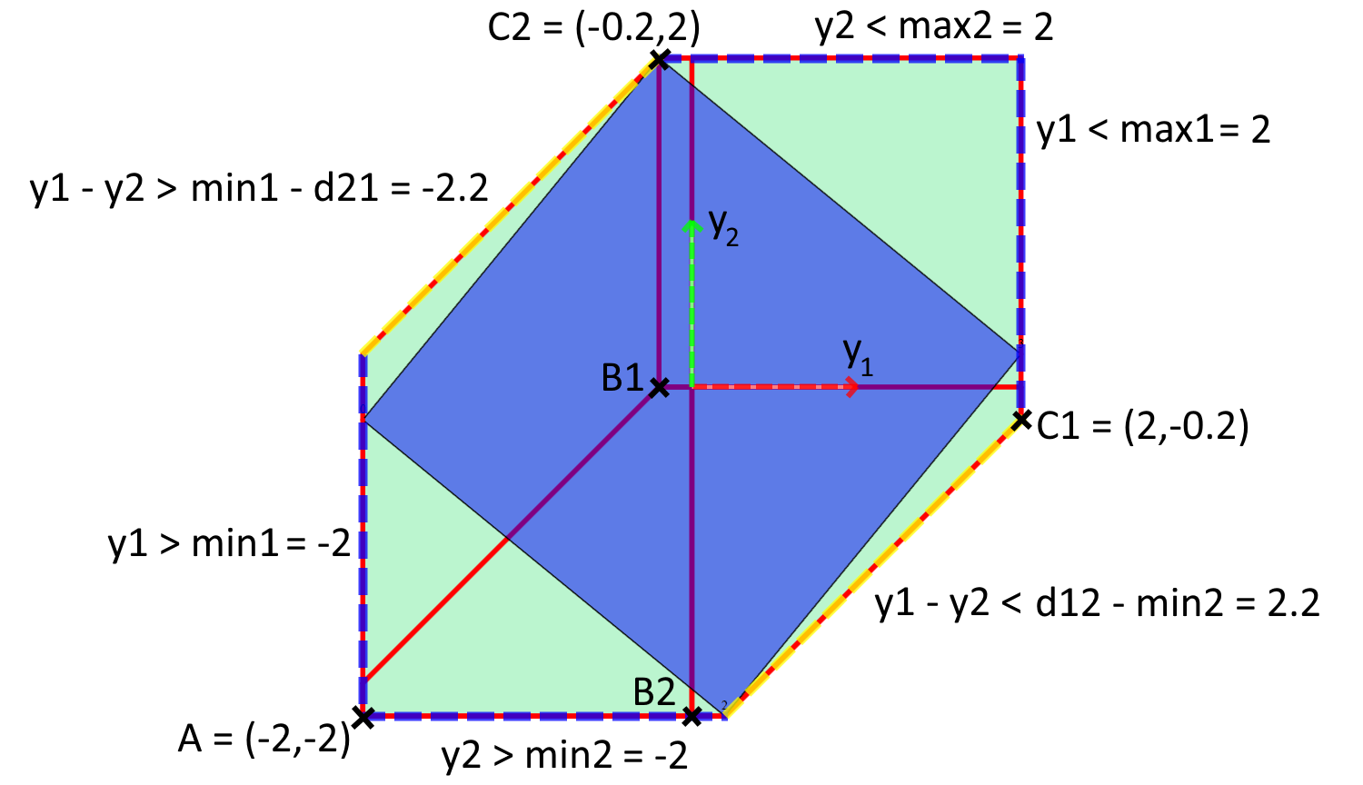
As $c_{1,1}=2$ , $c_{1,2}=-0.2$ , $c_{2,1}=-0.2$ and $c_{2,2}=2$ , the extremal points are, in the $(x_{1},x_{2},y_{1},y_{2})$ coordinates:

A=\begin{pmatrix}-1\\ -1\\ -2\\ -2\end{pmatrix}

B_{1}=\begin{pmatrix}1\\ -1\\ -0.2\\ 0\end{pmatrix}

B_{2}=\begin{pmatrix}-1\\ 1\\ 0\\ -2\end{pmatrix}

C_{1}=\begin{pmatrix}0.8\\ 1\\ 2\\ -0.2\end{pmatrix}

C_{2}=\begin{pmatrix}1\\ -1\\ -0.2\\ 2\end{pmatrix}

3.2 Octagon abstractions and $(\max,+,-)$ algebra

As in Section 3.1, we consider the abstraction of the image of an hypercube $K$ of $\mathbb{R}^{m}$ by an affine transformation $f:\mathbb{R}^{m}\to\mathbb{R}^{n}$ defined, for all $x\in\mathbb{R}^{m}$ and $i\in[1,n]$ , by $\big(f(x)\big)_{i}=\sum_{j=1}^{m}w_{i,j}x_{j}+b_{i}$ . But we consider here the abstraction of this image by an octagon, we will thus add some constraints on sums of variables to the abstraction computed in Section 3.1.

Proposition 4 (Optimal approximation of a linear layer by an octagon)

Let $K\subset\mathbb{R}^{m}$ be an hypercube defined as $K=\prod_{j}[\underline{x}_{j},\overline{x}_{j}]$ , with $\underline{x}_{j},\overline{x}_{j}\in\mathbb{R}$ . The tightest octagon of $\mathbb{R}^{m}\times\mathbb{R}^{n}$ containing

S:=\Big\{\big(x,f(x)\big)\,\Big|\,x\in K\Big\}

is the set of all $(x,y)\in\mathbb{R}^{m}\times\mathbb{R}^{n}$ satisfying

		$\displaystyle\Bigg(\bigwedge_{1\leq j\leq m}\underline{x}_{j}\leq x_{j}\leq\overline{x}_{j}\Bigg)\wedge\Bigg(\bigwedge_{1\leq i\leq n}m_{i}\leq y_{i}\leq M_{i}\Bigg)\wedge\Bigg(\bigwedge_{1\leq i_{1},i_{2}\leq m}y_{i_{1}}-y_{i_{2}}\leq\Delta_{i_{1},i_{2}}\Bigg)$
	$\displaystyle\wedge$	$\displaystyle\Bigg(\bigwedge_{1\leq i_{1},i_{2}\leq n}L_{i_{1},i_{2}}\leq y_{i_{1}}+y_{i_{2}}\leq\Gamma_{i_{1},i_{2}}\Bigg)$
	$\displaystyle\wedge$	$\displaystyle\Bigg(\bigwedge_{1\leq i\leq n,1\leq j\leq m}m_{i}-\overline{x}_{j}+\delta_{i,j}\leq y_{i}-x_{j}\leq M_{i}-\underline{x}_{j}-\delta_{i,j}\Bigg)$
	$\displaystyle\wedge$	$\displaystyle\Bigg(\bigwedge_{i,j}m_{i}+\underline{x}_{j}+\gamma_{i,j}\leq y_{i}+x_{j}\leq M_{i}+\overline{x}_{j}-\gamma_{i,j}\Bigg)$

where $m_{i},M_{i},\delta_{i,j},\Delta_{i_{1},i_{2}}$ are defined as in Proposition 3, and

	$\displaystyle\Gamma_{i_{1},i_{2}}$	$\displaystyle:=\sum_{w_{i_{1},j}+w_{i_{2},j}<0}\underline{x}_{j}(w_{i_{1},j}+w_{i_{2},j})+\sum_{w_{i_{1},j}+w_{i_{2},j}>0}\overline{x}_{j}(w_{i_{1},j}+w_{i_{2},j})$
	$\displaystyle L_{i_{1},i_{2}}$	$\displaystyle:=\sum_{w_{i_{1},j}+w_{i_{2},j}<0}\overline{x}_{j}(w_{i_{1},j}+w_{i_{2},j})+\sum_{w_{i_{1},j}+w_{i_{2},j}>0}\underline{x}_{j}(w_{i_{1},j}+w_{i_{2},j})$
	$\displaystyle\gamma_{i,j}$	$\displaystyle:=\begin{cases}0,&\text{if}\ 0\leq w_{i,j}\\ -w_{i,j}(\overline{x}_{j}-\underline{x}_{j}),&\text{if}\ -1\leq w_{i,j}\leq 0\\ (\overline{x}_{j}-\underline{x}_{j}),&\text{if}\ w_{i,j}\leq-1\end{cases}$

The proof is given in Appendix 0.C.

With the notations of Proposition 4, we have

Proposition 5

Let $M$ be the (classically) linear manifold in $\mathbb{R}^{m}\times\mathbb{R}^{n}\times\mathbb{R}^{m}\times\mathbb{R}^{n}$ defined by $(x^{+},y^{+},x^{-},y^{-})\in M$ if and only if $x^{+}+x^{-}=0$ and $y^{+}+y^{-}=0$ . The octagon $S$ defined in Proposition 4 is equal to the intersection of $M$ with the tropical convex polyhedron generated by the $1+2n+2m$ points $A,B^{+}_{1},\dots,B^{+}_{m},B^{-}_{1},\dots,B^{-}_{m},C^{+}_{1},\dots,C^{+}_{n},C^{-}_{1},\dots,C^{-}_{n}$ , where

A\,=(\underline{x}_{1},\dots,\underline{x}_{m},m_{1},\dots,m_{n},-\overline{x}_{1},\dots,-\overline{x}_{m},-M_{1},\dots,-M_{n})

$\displaystyle B^{+}_{k}$	$\displaystyle=(0,x^{+},y^{+},x^{-},y^{-})\text{ with}$	$\displaystyle x^{+}_{k}=\overline{x}_{k},$	$\displaystyle x^{+}_{j\neq k}=\underline{x}_{j},$	$\displaystyle y^{+}_{i}=m_{i}+\delta_{i,k}$
	$\displaystyle x_{k}^{-}=-\overline{x}_{k},$	$\displaystyle x^{-}_{j\neq k}=-\overline{x}_{j},$	$\displaystyle y^{-}_{i}=-M_{i}+\gamma_{i,k}$
$\displaystyle B^{-}_{k}$	$\displaystyle=(0,x^{+},y^{+},x^{-},y^{-})\text{ with}$	$\displaystyle x^{-}_{k}=-\underline{x}_{k},$	$\displaystyle x^{-}_{j\neq k}=-\overline{x}_{j},$	$\displaystyle y^{-}_{i}=-M_{i}+\delta_{i,k}$
	$\displaystyle x_{k}^{+}=\underline{x}_{k},$	$\displaystyle x^{+}_{j\neq k}=\underline{x}_{j},$	$\displaystyle y^{+}_{i}=m_{i}+\gamma_{i,k}$
$\displaystyle C^{+}_{l}$	$\displaystyle=(0,x^{+},y^{+},x^{-},y^{-})\text{ with}$	$\displaystyle y^{+}_{l}=M_{l},$	$\displaystyle y^{+}_{i\neq l}=M_{l}-\Delta_{l,i},$	$\displaystyle x^{+}_{j}=\underline{x}_{j}+\delta_{l,j}$
	$\displaystyle y_{l}^{-}=-M_{l},$	$\displaystyle y^{-}_{i\neq l}=M_{l}-\Gamma_{l,i},$	$\displaystyle x^{-}_{j}=-\overline{x}_{j}+\gamma_{l,j}$
$\displaystyle C^{-}_{l}$	$\displaystyle=(0,x^{+},y^{+},x^{-},y^{-})\text{ with}$	$\displaystyle y^{-}_{l}=-m_{l},$	$\displaystyle y^{-}_{i\neq l}=-m_{l}-\Delta_{i,l},$	$\displaystyle x^{-}_{j}=-\overline{x}_{j}+\delta_{l,j}$
	$\displaystyle y_{l}^{+}=m_{l},$	$\displaystyle y^{+}_{i\neq l}=-m_{l}+L_{l,i},$	$\displaystyle x^{+}_{j}=\underline{x}_{j}+\gamma_{l,j}$

The proof is given in Appendix 0.D.

Example 9 (Running example)

For the example network of Example 1, the formulas of Proposition 4 give the following constraints:

		$\displaystyle-1\leq x_{1}\leq 1$
		$\displaystyle 0\leq x_{1}-h_{1}\leq 2$
		$\displaystyle-4\leq x_{1}+h_{1}\leq 2$
		$\displaystyle-2\leq x_{1}-h_{2}\leq 0$
		$\displaystyle-2\leq x_{1}+h_{2}\leq 4$
		$\displaystyle-1\leq x_{2}\leq 1$
		$\displaystyle-2\leq x_{2}-h_{1}\leq 4$
		$\displaystyle-2\leq x_{2}+h_{1}\leq 0$
		$\displaystyle-2\leq x_{2}-h_{2}\leq 0$
		$\displaystyle-2\leq x_{2}+h_{2}\leq 4$
		$\displaystyle-3\leq h_{1}\leq 1$
		$\displaystyle 0\leq h_{2}-h_{1}\leq 4$
		$\displaystyle-2\leq h_{2}+h_{1}\leq 2$
		$\displaystyle-1\leq h_{2}\leq 3$

And the internal description is given by Proposition 5, with the following extreme points, where coordinates are ordered as $(x_{1}^{+},x_{2}^{+},h_{1}^{+},h_{2}^{+},x_{1}^{-},x_{2}^{-},h_{1}^{-},h_{2}^{-})$ :

		$\displaystyle(-1,-1,-3,-1,-1,-1,-1,-3)$
		$\displaystyle(1,-1,-1,1,-1,-1,-1,-3)$
		$\displaystyle(-1,1,-3,1,-1,-1,1,-3)$
		$\displaystyle(-1,-1,-3,-1,-1,-1,-1,-3)$
		$\displaystyle(1,-1,1,1,-1,1,-1,-1)$
		$\displaystyle(1,1,-1,3,-1,-1,1,-3)$
		$\displaystyle(-1,-1,-3,-1,1,-1,1,-1)$
		$\displaystyle(-1,-1,-1,-1,-1,1,-1,-1)$
		$\displaystyle(-1,-1,-3,-1,-1,-1,-1,-3)$
		$\displaystyle(-1,1,-3,1,1,-1,3,-1)$
		$\displaystyle(-1,-1,-1,-1,1,1,1,1)$

From the extremal points for the octagon abstraction above, we get the extremal points for $(h_{1}^{+},h_{2}^{+})$ , discarding the non extremal ones: $(-3,-1)$ , $(1,1)$ and $(-1,3)$ . and for $(h_{1}^{+},h_{2}^{-})$ : $(-3,-3)$ , $(1,-1)$ and $(-1,1)$ giving the zone in cyan of Figure 3.

4 Validation of multi-layered neural networks

General algorithm

The method developed in Section 3 is the cornerstone of our algorithm for analysing neural networks. A ReLU neural net consists of a chain of two kinds of computations, one which applies a classical linear transformation to their inputs, and another one which applies a ReLU function. We have seen that the affine map transformation can be over-approximated using tropical polyhedra. ReLU being a tropical affine function, the ReLU transform is exact in tropical polyhedra. It is thus possible to use tropical polyhedra to represent reachable states for every node in the network, at least for one layer ReLU networks.

Example 10

We carry on with Example 1 and complete the final computations of Example 7. The external representation is given by the tropical linear inequalities of Example 7 together with inequalities $max(0,h_{1})\leq y_{1}\leq max(0,h_{1})$ and $max(0,h_{2})\leq y_{2}\leq max(0,h_{2})$ . Now the corresponding tropical polyhedron is generated by the linear tropical operator ReLU on each of the extremal points $A$ , $B_{1}$ , $B_{2}$ , $C_{1}$ and $C_{2}$ and gives the two extra (last) coordinates in the axes $(x_{1},x_{2},h_{1},h_{2},y_{1},y_{2})$ , $A^{\prime}=(-1,-1,-3,-1,0,0),\ B^{\prime}_{1}=(1,-1,-1,1,0,1),\ B^{\prime}_{2}=(-1,1,-3,1,0,1),\ C^{\prime}_{1}=(-1,-1,1,1,1,1),\ C^{\prime}_{2}=(-1,1,-1,3,0,3)$ . The projections of theses 5 extreme points on $(h_{1},y_{2})$ give the points $(0,0)$ , $(0,1)$ , $(1,1)$ , $(0,3)$ among which $(0,1)$ is in the convex hull of $A^{\prime}=(0,0)$ , $B^{\prime}_{2}=B_{2}=(1,1)$ and $B^{\prime}_{1}=(0,3)$ represented in Figure 3(a).

The polyhedron given by the method of Section 3 only gives relations between 2 layers (the input and the first hidden layer). In order to get a polyhedron that represents the whole network when combining with e.g. another layer, we need to embed the first polyhedron from a space that represents only 2 layers to a higher space that represents the complete network, with one dimension per node. We will then need to intersect the polyhedra generated by each pair of layers to get the final result. Finally, as we are only interested in the input-output abstraction of the whole network, we can reduce computing costs by removing the dimensions corresponding to middle layers once those are calculated.

To this end, we use the following notations. Let $\mathcal{L}\subset\{L_{0},\ldots,L_{N}\}$ be a set of layers, layer $i$ containing $n_{i+1}$ neurons as in Definition 2. Let $n$ be the sum of all $n_{i+1}$ , with $i$ such that $L_{i}\in\mathcal{L}$ and $\mathcal{S}_{\mathcal{L}}\equiv\mathbb{R}_{max}^{n}$ be the tropical space in which we are going to interpret the values of the neurons on layers in $\mathcal{L}$ , with each dimension of $\mathcal{S}_{\mathcal{L}}$ corresponding to a node of a layer of $\mathcal{L}$ .

For $\mathcal{L}_{1},\mathcal{L}_{2}\subset\{L_{0},\ldots,L_{N}\}$ , for $\mathcal{H}\subset\mathcal{S}_{\mathcal{L}_{1}}$ a tropical polyhedron, we denote by $Proj(\mathcal{H},\mathcal{L}_{2})\subset\mathcal{S}_{\mathcal{L}_{2}}$ the projection of $\mathcal{H}$ onto $\mathcal{S}_{\mathcal{L}_{2}}$ when $\mathcal{S}_{\mathcal{L}_{2}}\subseteq\mathcal{S}_{\mathcal{L}_{1}}$ and let $Emb(\mathcal{H},\mathcal{L}_{2})\subset\mathcal{S}_{\mathcal{L}_{2}}$ be the embedding of $\mathcal{H}$ into $\mathcal{S}_{\mathcal{L}_{2}}$ when $\mathcal{S}_{\mathcal{L}_{1}}\subseteq\mathcal{S}_{\mathcal{L}_{2}}$ .

The main steps of our algorithm for over-approximating the values of neurons in a multi-layer ReLU network are the following:

•

We start with an initial tropical polyhedron $\mathcal{H}_{0}\subset\mathcal{S}_{\{L_{0}\}}$ that represents the interval ranges of the input layer $L_{0}$ .
•
For each additional layer $L_{i+1}$ :
- –
  
  Calculate an enclosing hypercube $C_{i}$ for the nodes of layer $L_{i}$ , given the current abstraction $\mathcal{H}_{i}\subset\mathcal{S}_{\mathcal{L}_{i}}$ (Section 2.3).
- –
  
  Calculate the polyhedron $\mathcal{P}_{i+1}$ representing relationships between layer $L_{i}$ and the new layer $L_{i+1}$ , for nodes of layer $L_{i}$ taking values in $C_{i}$ , as described in Section 3: Theorem 3.1 for the external description, and Theorem 3.2 for the internal description.
- –
  
  Let $\mathcal{L}^{\prime}_{i+1}=\mathcal{L}_{i}\cup\{L_{i+1}\}$ . Calculate $\mathcal{P}^{\prime}_{i+1}=Emb(\mathcal{P}_{i+1},\mathcal{L}^{\prime}_{i+1})$ (see below).
- –
  
  Intersect $\mathcal{P}^{\prime}_{i+1}$ with the projection (using the internal description, see below) of the previous abstraction $\mathcal{H}_{i}$ to get $\mathcal{H}^{\prime}_{i+1}=Emb(\mathcal{H}_{i},\mathcal{L}^{\prime}_{i+1})\cap\mathcal{P}^{\prime}_{i+1}$ (using the external description).
- –
  
  Choose $\mathcal{L}_{i+1}\supset\{L_{i+1}\}$ , and calculate $\mathcal{H}_{i+1}=Proj(\mathcal{H}^{\prime}_{i+1},\mathcal{L}_{i+1})$ . Usually, we would use $\mathcal{L}_{i+1}=\{L_{0},L_{i+1}\}$ if we only want relations between the input and output layers, or $\mathcal{L}_{i+1}=\{L_{0},\ldots,L_{i+1}\}$ if we want relations between every layer.

We need now to describe the projection and embedding functions $Proj$ and $Emb$ . Let $\mathcal{L}_{2}\subset\mathcal{L}_{1}\subset\{L_{0},\ldots,L_{N}\}$ be two sets of layers. Let $\mathcal{H}$ be a polyhedron on $\mathcal{S}_{\mathcal{L}_{1}}$ . We have $\mathcal{H}^{\prime}=Proj(\mathcal{H},\mathcal{L}_{2})=\{(x_{i})_{L_{i}\in\mathcal{L}_{2}},(x_{i})_{L_{i}\in\mathcal{L}_{1}}\in\mathcal{H}\}$ , i.e. for each point in $\mathcal{H}$ , we only keep the dimensions corresponding to layers in $\mathcal{L}_{2}$ , and discard the other dimensions. Projecting is easy with the internal description of polyhedron, as we can project the extreme points of $\mathcal{H}$ to get generators of $\mathcal{H}^{\prime}$ . However, we do not have a simple algorithm to project the external description of a polyhedron.

Let $\mathcal{L}_{1}\subset\mathcal{L}_{2}\subset\{L_{0},\ldots,L_{N}\}$ be two sets of layers, and $\Delta$ be the sum of $n_{i+1}$ , the number of neurons of layer $L_{i}$ , for $i$ such that $L_{i}\in\mathcal{L}_{2}\setminus\mathcal{L}_{1}$ . Let $\mathcal{H}$ be a polyhedron on $\mathcal{S}_{\mathcal{L}_{1}}$ . We note that $\mathcal{S}_{2}\equiv\mathcal{S}_{1}\times\mathbb{R}_{max}^{\Delta}$ , and thus $\mathcal{H}^{\prime}=Emb(\mathcal{H},\mathcal{L}_{2})\equiv\mathcal{H}\times\mathbb{R}_{max}^{\Delta}$ , i.e. we add dimensions corresponding to each node in $\mathcal{L}_{2}$ which are not in $\mathcal{L}_{1}$ , and let points in $\mathcal{H}^{\prime}$ take any value of $\mathbb{R}_{max}$ on these dimensions. Embedding is based on simple matrices concatenations in the external description, see Appendix 0.F for more details. Embedding using the internal description is more involved and is explained after exemplifying things on a simple example.

Example 11

We consider the 1-layer neural net of Example 1, and add a second layer. The new linear layer is defined by $u_{1}=y_{2}-y_{1}-1$ , $u_{2}=y_{1}-y_{2}+1$ and the output neurons are $z_{1}=max(0,u_{1})=max(0,y_{2}-y_{1}-1)$ and $z_{2}=max(0,u_{2})=max(0,y_{1}-y_{2}+1)$ .

The enclosing cube for the tropical polyhedron ${\mathcal{H}}$ containing the values of neurons of the first layer $L_{1}$ : $y_{1}$ , $y_{2}$ of Example 1 is $[0,1]\times[0,3]$ . The analysis of the second layer $L_{2}$ , supposing its input belongs to $[0,1]\times[0,3]$ gives the constraint (an extract of the external representation of the resulting tropical polyhedron ${\mathcal{H}}^{\prime}$ ) $-3\leq u_{1}-y_{1}\leq 2,\ -2\leq u_{1}-y_{2}\leq-1,\ -2\leq u_{2}-y_{1}\leq 1,\ -5\leq u_{2}-y_{2}\leq 2,\ z_{1}=max(0,u_{1}),\ z_{2}=max(0,u_{2})$ . The intersection of the embedding $Emb({\mathcal{H}}^{\prime},\{L_{0},L_{1},L_{2}\})$ with the embedding $Emb({\mathcal{H}},\{L_{0},L_{1},L_{2}\})$ consists, as we saw above, in concatenating the tropical constraints, in the common space of variables. This implies in particular that we add the constraint $-3\leq y_{1}-y_{2}\leq 0$ to the above equations. The intersection is actually a zone intersection, where we have to normalize the corresponding DBM. A manual calculation shows that this will make use of the equalities $u_{2}-y_{2}=(u_{2}-y_{1})+(y_{1}-y_{2}),\ u_{1}-y_{1}=(u_{1}-y_{2})+(y_{2}-y_{1})$ . By combining equations, we get the refined bounds (refined lower bound for the first equation, refined upper bound for the second equation) $-2\leq u_{1}-y_{1}\leq 2,\ -5\leq u_{2}-y_{2}\leq 1$ .

Embedding a tropical polyhedron: internal description

In this paragraph, we embed a polyhedron into a higher dimensional space, using the internal description.

Suppose $\mathcal{H}$ is a tropical polyhedron in $\mathbb{R}^{n}$ (such as $\mathcal{P}_{i}$ in the previous section) that we want to embed $\mathcal{H}$ into a larger space, with an extra coordinate, which we consider bounded here within $[a,b]$ . So we need to determine a presentation of the tropical polyedron $\mathcal{H}^{\prime}=\mathcal{H}\times[a,b]$ .

Supposing we have $m$ extreme points $p_{i}$ for representing $\mathcal{H}$ , a naive method consists in noticing that the family $(p_{i},a),(p_{i},b)$ is a generator of $\mathcal{H}^{\prime}$ and removing non-extreme points from that list. But that would exhibit poor performance, as we get $m\times 2^{k}$ extreme points for $\mathcal{H}^{\prime\prime}$ . We can in fact do better:

Theorem 4.1

The extreme points of $\mathcal{H}^{\prime}$ are $\{(p_{i},a),1\leq i\leq m\}\cup\{(p_{i},b),i\in I\}$ , where $I$ is a subset of indexes of generators of $\mathcal{H}$ , $I\subset[1,m]$ , such that:

	$\displaystyle\forall i\in I,\forall j\in[1,m]\setminus\{i\},p_{i}\oplus p_{j}\neq p_{i}$		(5)
	$\displaystyle\forall i\in[1,m]\setminus I,\exists j\in[1,m]\setminus\{i\}\mbox{ s.t. }p_{i}\oplus p_{j}=p_{i}$		(6)

The proof is given in Appendix 0.G. Passing to the limit, this shows that the extreme points of $\mathcal{H}\times\mathbb{R}$ are $(p_{i},-\infty)$ , $i=1,\ldots,m$ and the extreme rays are $(p_{i},0)$ , $i\in I$ for the smallest $I$ verifying Equation 7. In the current implementation, we do not use extreme rays and embed $\mathcal{H}$ into larger state spaces by using large enough values for $a$ and $b$ .

Checking properties on ReLU neural nets

Given an affine guard

h(x,y)=\sum\limits_{i=1}^{m}h_{i}x_{i}+\sum\limits_{j=1}^{n}h^{\prime}_{j}y_{j}+c

where $x_{i}$ , resp. $y_{j}$ are the input, resp. output neurons, we want to determine whether, for all input values in $[-1,1]$ , we have $h(x)\geq 0$ (this can encode properties $(P_{1})$ and $(P_{2})$ of Example 1).

There are two ways to check such properties. The first one, that we have implemented, is as follows. We abstract the input output relation that the network under analysis encodes, using a tropical polyhedron ${\mathcal{H}}$ as described in Section 4. From this, we derive the smallest zone $Z$ containing ${\mathcal{H}}$ as in Section 2.3. Finally, we solve the linear programming problem $m=\min\limits_{x,y\in Z}h(x,y)$ using any classical algorithm (we used glpk in our prototype). This is enough for checking $(P_{1})$ in Example 1 since $m\geq 0$ proves our property true, but not $(P_{2})$ . The second way can be useful to check $(P_{2})$ : here we have no choice but try to solve $m=\min\limits_{x,y\in{\mathcal{H}}}h(x,y)$ which is not a convex optimization problem, in any sense (tropical nor classical). This could be encoded as MILP problem instead and is left for future work.

5 Improvements of the analysis

We will refine here the tropical abstractions we have defined in Section 3 by ”subdividing” the support of the functions we are approximating. Since we are linearizing tropical rational functions, we expect to be closer and closer to the actual graph of the function, by doing enough subdivisions.

We begin by showing how we can improve the abstraction of affine scalar functions $f$ , in the particular case where $m=n=1$ i.e. when $f$ goes from $\mathbb{R}$ to $\mathbb{R}$ , before we treat the much more involved general case in Theorem 5.2. Thus, we suppose first that we want to abstract the graph $\mathcal{G}_{f}$ of $f(x)=\lambda x+m$ , $x\in[a,b]$ , by a tropical polyhedron.

We can get a more precise result than what we got in Section 3, i.e. a smaller polyhedron that still contains all $\{(x,f(x))|x\in[a,b]\}$ by splitting the interval $[a,b]$ in $N$ sub-intervals $[c_{k},c_{k+1}]$ , with $c_{0}=a$ and $c_{N}=b$ and calculating an over-approximation of $f$ on each sub-interval, and returning the tropical union of all these polyhedra. In fact, we can give again explicit external and internal representations of these unions of tropical polyhedra as follows.

Theorem 5.1

A sound abstraction as a tropical polyhedron $\mathcal{P}$ of the graph $\mathcal{G}_{f}$ of $f$ over $[a,b]$ given by subdividing the domain in $N$ sub-intervals has the following external representation of $N+2$ tropical inequalities, $\mathcal{P}$ is defined by depending on the value of $\lambda$ :

•

If $\lambda\leq 0$ , we add the $N-1$ constraints $0\leq\max(x-c_{k},y-f(c_{k}))$ for $k=1,\ldots,N-1$ , to the ones of Theorem 3.1, i.e. $a\leq x$ , $f(b)\leq y$ and $max(x-b,y-f(a))\leq 0$
•

If $0\leq\lambda\leq 1$ , we add the $N-1$ constraints $y-f(c_{k})\leq\max(0,x-c_{k})$ for $k=1,\ldots,N-1$ , to the ones of Theorem 3.1, i.e. $y-f(a)\leq x-a$ , $y-f(b)\leq 0$ and $max(x-b+f(b),f(a))\leq y$
•

If $\lambda\geq 1$ , we add the $N-1$ constraints $x-c_{k}\leq\max(0,y-f(c_{k}))$ for $k=1,\ldots,N-1$ , to the ones of Theorem 3.1, i.e. $\max(y-f(b)+b,a)\leq x$ , $x\leq b$ , $x-a\leq f(x)-f(a)$ .

$\mathcal{P}$ can also be internally represented as the tropical convex hull of at most $N+2$ extreme points $A$ , $B$ and $C_{i}$ , $i\in[1,N]$ with $A=(a,f(a))$ , $B=(b,f(b))$ , and $C$ is $(c_{i-1},f(c_{i}))$ if $\lambda\leq 0$ , $(c_{i-1}+f(c_{i})-f(c_{i-1}),f(c_{i}))$ if $0\leq\lambda\leq 1$ and $(c_{i},f(c_{i-1})+c_{i}-c_{i-1})$ if $\lambda\geq 1$ .

Proof

Take any $k$ in $[0,N-1]$ . Consider first the case $\lambda\leq 0$ . Now if $x\leq c_{k}$ , then $f(x)\geq f(c_{k})$ , and if $x\geq c_{k}$ , then $f(x)\leq f(c_{k})$ . Therefore $0\leq\max(x-c_{k},f(x)-f(c_{k}))$ .

Now, suppose $0\leq\lambda\leq 1$ . If $x\leq c_{k}$ , then $f(x)\leq f(c_{k})$ , otherwise if $x\geq c_{k}$ , then $f(x)-f(c_{k})\leq x-c_{k}$ , and we conclude that $f(x)-f(c_{k})\leq\max(0,x-c_{k})$ .

Finally, we consider the case $\lambda\geq 1$ . If $x\leq c_{k}$ , then $f(x)\leq f(c_{k})$ , whereas if $x\geq c_{k}$ , then $f(x)-f(c_{k})\geq x-c_{k}$ . This means that $x-c_{k}\leq\max(0,f(x)-f(c_{k}))$ .

Compare Figure 7 with Figure 4 to see the improvement due to subdivision. Still, the tropical inequalities that we added using subdivisions give more precision on only ”one side” of the polyhedron. This will not be the case with the abstraction based on the octagon abstraction of Section 3.2.

Now we are considering the general case where $f$ is an affine function from $\mathbb{R}^{m}$ to $\mathbb{R}^{n}$ . We consider here subdivisions $c^{0}_{i}=a_{i},\ldots c^{N}_{i}=b_{i}$ of intervals $[a_{i},b_{i}]$ , $i=1,\ldots,m$ in $N$ subintervals, and want to generalize the previous result to this higher dimensional case. Contrarily to the previous case ( $f:\mathbb{R}\rightarrow\mathbb{R}$ ), we have no explicit external nor internal representation for the tropical polyhedron, union of the tropical polyhedra, abstraction of the graph of $f$ over each subdomain using Theorem 3.1. We could still take their unions, as a tropical polyhedron, using the double description method [2]. In the sequel, we describe a sound abstraction of this union, as a tropical polyhedron, that is generally sufficient for our purpose and does not need the computational complexity of the double description method.

Theorem 5.2

A sound and tighter over-approximation of $\mathcal{G}_{f}$ than the one of Theorem 3.1 is given externally by the tropical constraints of Theorem 3.1 plus the following constraints, for any subdivision $c^{0}_{i}=a_{i},\ldots c^{N}_{i}=b_{i}$ of intervals $[a_{i},b_{i}]$ , $i=1,\ldots,m$ in $N$ subintervals:

•

If $\lambda_{i,j}\leq 0$ , then we add the constraint $0\leq\max(x_{i}-c^{k}_{i},y_{j}-m_{j}+\lambda_{i,j}(b_{i}-c^{k}_{i}))$ . Otherwise if $0\leq\lambda_{i,j}\leq 1$ , we add the constraint $y_{j}-M_{j}+\lambda_{i,j}(b_{i}-c^{k}_{i})\leq\max(0,x_{i}-c^{k}_{i})$ . And finally, we add $x_{i}-c^{k}_{i}\leq\max(0,y_{j}-m_{j}-\lambda_{i,j}(c^{k}_{i}-a_{i}))$ if $\lambda_{i,j}\geq 1$ .
•

Let $I_{j-}\subset[1,m]$ , maximal, such as for all $i\in I_{j-}$ , $\lambda_{i,j}\leq 0$ . We write $\sigma_{j-}=\sum\limits_{i\in I_{j-}}\lambda_{i,j}(b_{i}-c^{k}_{i})$ . Then, we add the constraint $0\leq\max(y_{j}-m_{j}+\sigma_{j-},\max\limits_{i\in I_{j-}}(x_{i}-c^{k}_{i}))$ .
•

Let $I_{j0}\subset[1,m]$ , maximal, such as for all $i\in I_{j0}$ , $0\leq\lambda_{i,j}\leq 1$ and $\sum\limits_{i\in I_{j0}}\lambda_{i,j}\leq 1$ and let $\sigma_{j0}=\sum\limits_{i\in I_{j0}}\lambda_{i,j}(b_{i}-c^{k}_{i})$ . Then we add the constraint $y_{j}-M_{j}+\sigma_{j0}\leq\max(0,\max\limits_{i\in I_{j0}}(x_{i}-c^{k}_{i}))$ .
•

Finally, for any $J$ subset of $[1,n]$ , let $\sigma_{i,J}=\sum\limits_{j\in J}\lambda_{i,j}$ and $m_{J}=\sigma_{0,J}+\sum\limits_{\sigma_{i,J}<0}\sigma_{i,J}b_{i}+\sum\limits_{\sigma_{i,J}>0}\sigma_{i,J}a_{i}$ . For $j\in J$ , let $u_{j}\in[m_{j},M_{j}]$ such as $\sum\limits_{j\in J}u_{j}=m_{J}$ : we add the constraint $0\leq\max_{j\in J}(y_{j}-u_{j})$

We exemplify this in Figures 8 and 9. The proof is given in Appendix 0.I.

6 Implementation, experiments and benchmarks

Internal, external and double description methods

Overall, we have developed methods for propagating an outer-approximation of the values that the different layers of neurons can take, within a MLP with ReLU activation. Let us discuss the pros and cons of using the internal description, external description and double description methods:

•

The double description method allows for possibly using subdivisions, propagating values in multiple layers and projecting them onto a subset of interesting neurons (e.g. input and output layers), as well as computing an enclosing zone, for synthesizing classification properties. We have implemented this in a prototype using Polymake [19], whose results we briefly discuss below.
•

The internal description allows for analyzing one layer networks, using subdivisions, project onto an interesting subset of neurons, as well as computing an enclosing zone (Section 2.3). We have implemented this method in C++ in a standalone prototype, nntrop, that takes as input a Sherlock file [15] describing the one hidden layer neural net to analyze plus a linear formula to be checked, and returns the tropical abstraction of the values that neurons can take, its over-approximation by a zone, and whether the linear specification is satisfied or not.
•

The external description allows for analyzing multiple layer networks (see Section 4).

The double description method is much more expensive since the translation between the internal and external representations may be quite complex.

Experiments and benchmarks

We briefly compare the computation times between internal description only and double description in Table 1. For each example, we indicate in the columns # inp. the number of input neurons, # out. the number of output neurons, # hid. the number of hidden layers, # neur. is the total number of neurons (input, output and hidden), t. intern is the time spent for computing the internal representation and t. double for the double description of the tropical polyhedron abstracting the corresponding neural net. Experiments are performed on a simple computer with ArchLinux and a Intel(R) Core(TM) i5-7200U CPU @ 2.50GHz.

We of course see the influence of a potential exponential complexity for going back and forth between internal and external descriptions, but also the fact that we relied on a perl (interpreted) implementation of tropical polyhedra (the one of polymake [19], with exact rational arithmetics), which is much slower than the C++ implementation we wrote for the internal description method (although the internal description method does work in a twice as big space because it considers the octagon instead of just zone abstraction).

Table 1: Execution times (internal and double description) on sample networks.

Example	# inp.	# out.	# hid.	# neur.	t. intern. (s)	t. double (s)
running	2	2	0	4	0.006	1.83
running2	2	2	1	6	0.011	4.34
multi	2	8	1	13	0.005	3.9
krelu	2	2	0	4	0.011	1.94
tora_modified_controller	4	1	1	6	0.005	14.57
tora_modified_controller_1	4	1	1	105	0.75	815.12
quadcopter_trial_controller_3	18	1	1	49	0.009	102.54
quadcopter_trial_controller_1	18	1	1	69	0.2	469.77
quad_modified_controller	18	1	1	20	0.005	14
car_nn_controller_2	4	2	1	506	104.75	–
car_nn_controller_1	4	2	1	506	88.8	–
ex	2	1	5	59	0.195	1682.28

In Table 1, running is the network of Example 1, and running2 is the extension with an extra layer of Example 11, discussed in great length in these examples. Example krelu is the running example from [36] that we discuss at the end of this section, and tora_modified_controller, tora_modified_controller_1, quadcopter_trial_controller_3, quadcopter_trial_controller_1, quad_modified_controller, car_nn_controller_2, car_nn_controller_1 and ex are examples from the distribution of Sherlock [15]. ex is a multi-layer example for which the algorithm using only the internal representation does not compute the intersection of tropical polyhedra between layers (involving the external representation), contrarily to the double description prototype. We now discuss some of these examples below.

Network multi is a simple 2-layer, 13 neurons example with inputs $x_{1},\ x_{2}$ , outputs $y_{1},y_{2},\ldots,y_{8}$ and

$\begin{bmatrix}h_{1}\\ h_{2}\\ h_{3}\end{bmatrix}=ReLU\begin{pmatrix}\begin{bmatrix}1&1\\ 1&-1\\ -1&-1\end{bmatrix}\begin{bmatrix}x_{1}\\ x_{2}\end{bmatrix}\end{pmatrix}$ , $\begin{bmatrix}y_{1}\\ y_{2}\\ y_{3}\\ y_{4}\\ y_{5}\\ y_{6}\\ y_{7}\\ y_{8}\end{bmatrix}=max\left(\begin{pmatrix}\begin{bmatrix}1&1&1\\ 1&1&-1\\ 1&-1&1\\ 1&-1&-1\\ -1&1&1\\ -1&1&-1\\ -1&-1&1\\ -1&-1&-1\end{bmatrix}\begin{bmatrix}h_{1}\\ h_{2}\\ h_{3}\end{bmatrix}\end{pmatrix},0\right)$ . Our zone based abstraction returns the following ranges: $y_{1}\in[0,6]$ , $y_{2}\in[0,4]$ , $y_{3}\in[0,4]$ , $y_{4}\in[0,2]$ , $y_{5}\in[0,4]$ , $y_{6}\in[0,2]$ , $y_{5}\in[0,2]$ and $y_{8}=0$ , whereas the exact ranges for $y_{1}$ to $y_{7}$ is $[0,2]$ . Our algorithm is thus exact for $y_{4}$ , $y_{6}$ , $y_{7}$ and $y_{8}$ but not $y_{1}$ , $y_{2}$ , $y_{3}$ nor $y_{5}$ . This is due to the fact that the zone-based tropical abstraction does represent faithfully the differences of neuron values, but not sums in particular. For instance, $y_{2}=max(0,2x_{1})$ which cannot be represented exactly by our method.

Network krelu is a 2 layer 4 neurons example from [36]. We get the correct bounds on the outputs: $0\leq z_{1},z_{2}\leq 2$ , as well as relations between the inputs and the outputs: $z_{j}\leq x_{i}+1$ . However, we do not have significant relations between $z_{1}$ and $z_{2}$ , as those are not tropically linear. We refer to the results obtained with 1-ReLU and 2-ReLU in [36]: they both get better relations between $z_{1}$ and $z_{2}$ , in particular $z_{1}+z_{2}\leq 2$ which is not representable in a tropical manner (except by using an octagon based abstraction, which is outside the scope of this paper). However 1-ReLU does not keep track of relations between the inputs and the outputs, and has sub-optimal relations between the outputs, as it cannot represent the non linear ReLU function exactly. 2-ReLU, on the other hand gets both the relation between the output variables, and between the inputs and outputs correct, but is more computationally expensive.

In order to assess the efficiency of the internal description methods, we have run a number of experiments, with various number of inputs and ouputs for neural nets with one hidden layer only. The linear layers are generated randomly, with weights between -2 and 2. For 100 inputs and 100 neurons in the hidden layer, the full pipeline (checking the linear specification in particular) took about 35 seconds, among which the tropical polyhedron analysis took 6 seconds. Timings are shown in the figure on the right (demonstrating the expected complexity, cubical in the number of neurons), where the x-axis is number of input neurons, y-axis is the number of output neurons, and z-axis is time.

7 Conclusion and future work

We have explored the use of tropical polyhedra as a way to circumvent the combinatorial complexity of neural networks with ReLU activation function. The first experiments we made show that our approximations are tractable when we are able to use either the internal or the external representations for tropical polyhedra, and not both at the same time. This is akin to the results obtained in the classical polyhedron approach, where most of the time, only a sub polyhedral domain is implemented, needing only one of the two kinds of representations. It is interesting to notice that a recent paper explores the use of octohedral constraints, a three-dimensional counterpart of our octagonal representations, in the search of more tractable yet efficient abstraction for ReLU neural nets [32]. This work is a first step towards a hierarchy of approximations for ReLU MLPs. We have been approximating the tropical rational functions that these neural nets compute by tropical affine functions, and the natural continuation of this work is to go for higher-order approximants, in the tropical world. We also believe that the tropical approach to abstracting ReLU neural networks would be particularly well suited to verification of ternary nets [28]. These ternary nets have gained importance, in particular in embedded systems: simpler weights mean smaller memory needs and faster evaluation, and it has been observed [1] that they can provide similar performance to general networks.

References

[1] Hande Alemdar, Nicholas Caldwell, Vincent Leroy, Adrien Prost-Boucle, and Frédéric Pétrot. Ternary neural networks for resource-efficient AI applications. CoRR, abs/1609.00222, 2016.
[2] X. Allamigeon, S.Gaubert, and E. Goubault. The tropical double description method. 27th International Symposium on Theoretical Aspects of Computer Science, STACS 2010.
[3] Xavier Allamigeon. Static analysis of memory manipulations by abstract interpretation - Algorithmics of tropical polyhedra, and application to abstract interpretation. PhD thesis, École Polytechnique, Palaiseau, France, 2009.
[4] Xavier Allamigeon, Stephane Gaubert, and Eric Goubault. Inferring min and max invariants using max-plus polyhedra. In Maria Alpuente and Germain Vidal, editors, Static Analysis, 15th International Symposium, SAS 2008, Valencia, Spain, July 16-18, 2008. Proceedings, volume 5079 of Lecture Notes in Computer Science, pages 189–204. Springer, 2008.
[5] Xavier Allamigeon, Stéphane Gaubert, and E. Goubault. Computing the vertices of tropical polyhedra using directed hypergraphs. Discrete and Computational Geometry, 49, 04 2009.
[6] Stanley Bak, Hoang-Dung Tran, Kerianne Hobbs, and Taylor T. Johnson. Improved geometric path enumeration for verifying relu neural networks. In Shuvendu K. Lahiri and Chao Wang, editors, Computer Aided Verification. Springer International Publishing, 2020.
[7] O. Bastani, Y. Ioannou, L. Lampropoulos, D. Vytiniotis, A. Nori, and A. Criminisi. Measuring neural net robustness with constraints,” in advances in neural information processing systems (nips), 2016.
[8] B. Blanchet, P. Cousot, R. Cousot, J. Feret, L. Mauborgne, A. Miné, D. Monniaux, and X. Rival. A static analyzer for large safety-critical software. In PLDI, pages 196–207. ACM Press, June 2003.
[9] Elena Botoeva, Panagiotis Kouvaros, Jan Kronqvist, Alessio Lomuscio, and Ruth Misener. Efficient verification of relu-based neural networks via dependency analysis. Proceedings of the AAAI Conference on Artificial Intelligence, 34(04):3291–3299, 2020.
[10] François Bourdoncle. Abstract interpretation by dynamic partitioning. JOURNAL OF FUNCTIONAL PROGRAMMING, 2, 1992.
[11] Patrick Cousot and Radhia Cousot. Abstract interpretation: A unified lattice model for static analysis of programs by construction or approximation of fixpoints. In Conference Record of the Fourth ACM Symposium on Principles of Programming Languages, Los Angeles, California, USA, January 1977, pages 238–252, 1977.
[12] Patrick Cousot and Radhia Cousot. Abstract interpretation: A unified lattice model for static analysis of programs by construction or approximation of fixpoints. In POPL. ACM, 1977.
[13] Patrick Cousot and Nicolas Halbwachs. Automatic discovery of linear restraints among variables of a program. In Proceedings of the 5th ACM SIGACT-SIGPLAN Symposium on Principles of Programming Languages, POPL ’78, page 84–96, New York, NY, USA, 1978. Association for Computing Machinery.
[14] S. Dutta, X. Chen, and S. Sankaranarayanan. Reachability analysis for neural feedback systems using regressive polynomial rule inference. In HSCC, 2019.
[15] Souradeep Dutta, Xin Chen, Susmit Jha, Sriram Sankaranarayanan, and Ashish Tiwari. Sherlock - A tool for verification of neural network feedback systems: demo abstract. In HSCC, 2019.
[16] Rüdiger Ehlers. Formal verification of piece-wise linear feed-forward neural networks. In ATVA, 2017.
[17] Ivan Evtimov, Kevin Eykholt, Earlence Fernandes, Tadayoshi Kohno, Bo Li, Atul Prakash, Amir Rahmati, and Dawn Song. Robust physical-world attacks on machine learning models. CoRR, abs/1707.08945, 2017.
[18] S. Gaubert and R. Katz. The minkowski theorem for max-plus convex sets. Linear Algebra and Appl., 421:356––369, 2006.
[19] Ewgenij Gawrilow and Michael Joswig. polymake: a Framework for Analyzing Convex Polytopes, pages 43–73. Birkhäuser Basel, 2000.
[20] T. Gehr, M. Mirman, D. Drachsler-Cohen, P. Tsankov, S. Chaudhuri, and M. Vechev. AI2: Safety and robustness certification of neural networks with abstract interpretation. Conférence IEEE S&P 2018, 2018.
[21] Sven Gowal, Krishnamurthy Dvijotham, Robert Stanforth, Rudy Bunel, Chongli Qin, Jonathan Uesato, Relja Arandjelovic, Timothy A. Mann, and Pushmeet Kohli. On the effectiveness of interval bound propagation for training verifiably robust models. CoRR, abs/1810.12715, 2018.
[22] Patrick Henriksen and Alessio R. Lomuscio. Efficient neural network verification via adaptive refinement and adversarial search. In ECAI, volume 325 of Frontiers in Artificial Intelligence and Applications, 2020.
[23] X. Huang, M. Kwiatkowska, S. Wang, and M. Wu. Safety verification of deep neural networks. International Conference on Computer Aided Verification, 2017.
[24] Kyle Julian, Mykel J. Kochenderfer, and Michael P. Owen. Deep neural network compression for aircraft collision avoidance systems. AIAA Journal of Guidance, Control, and Dynamics, 2018. Cf. https://arxiv.org/pdf/1810.04240.pdf.
[25] G. Katz, C. Barrett, D. L. Dill, K. Julian, and M. J. Kochenderfer. Reluplex: An efficient smt solver for verifying deep neural networks. CAV 2017.
[26] Guy Katz, Derek A. Huang, Duligur Ibeling, Kyle Julian, Christopher Lazarus, Rachel Lim, Parth Shah, Shantanu Thakoor, Haoze Wu, Aleksandar Zeljić, David L. Dill, Mykel J. Kochenderfer, and Clark Barrett. The Marabou framework for verification and analysis of deep neural networks. In Computer Aided Verification, pages 443–452. Springer, 2019.
[27] Haitham Khedr, James Ferlez, and Yasser Shoukry. Effective formal verification of neural networks using the geometry of linear regions, 2020.
[28] Fengfu Li and Bin Liu. Ternary weight networks. CoRR, abs/1605.04711, 2016.
[29] Laurent Mauborgne and Xavier Rival. Trace partitioning in abstract interpretation based static analyzers. In Programming Languages and Systems, 2005.
[30] Antoine Miné. A new numerical abstract domain based on difference- bound matrices. In PADO II, volume LNCS 2053, 2001.
[31] Antoine Miné. The octagon abstract domain. High. Order Symb. Comput., 19(1):31–100, 2006.
[32] Mark Niklas Müller, Gleb Makarchuk, Gagandeep Singh, Markus Püschel, and Martin Vechev. Precise multi-neuron abstractions for neural network certification, 2021.
[33] W. Ruan, X. Huang, and M. Kwiatkowska. Reachability analysis of deep neural networks with provable guarantees. In IJCAI, 2018.
[34] Wang Shiqi, Kexin Pei, Whitehouse Justin, Junfeng Yang, and Suman Jana. Efficient formal safety analysis of neural networks. In NIPS, 2018.
[35] G. Singh, T. Gehr, M. Mirman, M. Püschel, and M. Vechev. Fast and effective robustness certification.
[36] Gagandeep Singh, Rupanshu Ganvir, Markus Püschel, and Martin Vechev. Beyond the single neuron convex barrier for neural network certification. In Advances in Neural Information Processing Systems (NeurIPS). 2019.
[37] Gagandeep Singh, Timon Gehr, Markus Püschel, and Martin Vechev. An abstract domain for certifying neural networks. Proc. ACM Program. Lang., 3(POPL), January 2019.
[38] Gagandeep Singh, Timon Gehr, Markus Püschel, and Martin Vechev. Boosting robustness certification of neural networks. In ICLR. 2019.
[39] Christian Szegedy, Wojciech Zaremba, Ilya Sutskever, Joan Bruna, Dumitru Erhan, Ian Goodfellow, and Rob Fergus. Intriguing properties of neural networks. 2013.
[40] V. Tjeng, K. Xiao, and R. Tedrake. Evaluating robustness of neural networks with mixed integer programming.
[41] S. Wang, K. Pei, J. Whitehouse, J. Yang, and S. Jana. Formal security analysis of neural networks using symbolic intervals. USENIX Security), 2018.
[42] Huan Zhang, Hongge Chen, Chaowei Xiao, Sven Gowal, Robert Stanforth, Bo Li, Duane Boning, and Cho-Jui Hsieh. Towards stable and efficient training of verifiably robust neural networks. In ICLR, 2020.
[43] L. Zhang, G.Naitzat, and L.-H. Lim. Tropical geometry of deep neural networks. Proceedings of the 35th International Conference on Machine Learning, PMLR 80:5824-5832, 2018.

Appendix 0.A Proof of Proposition 1

Proof

We begin by proving that $H_{int}\subset H_{ext}$ . For this, we only need to prove that the generators are in $H_{ext}$ .

For all $i$ and $j$ such that $0\leq i,j\leq n$ , we know that $c_{0,i}+c_{i,j}\geq c_{0,j}$ as the zone representation we started with is closed. Thus $a_{i}-a_{j}=-c_{0,i}+c_{0,j}\leq c_{i,j}$ and $A\in H_{ext}$ .

Similarly, for all $k\in[1,n]$ , we have $b_{k,i}-b_{k,j}=(c_{k,0}-c_{k,i})-(c_{k,0}-c_{k,j})=-c_{k,i}+c_{k,j}\leq c_{i,j}$ as the initial zone is closed, hence $B_{k}\in H_{ext}$ .

We then prove that $H_{ext}\subset H_{int}$ . Let $x=(x_{1},\dots,x_{n})\in H_{ext}$ . We define $x^{\prime}=(x^{\prime}_{i})_{1\leq i\leq n}$ by

x^{\prime}_{i}=\max(a_{i},\max_{k}(x_{k}-c_{k,i})).

Noting that we can rewrite

x^{\prime}_{i}=\max(a_{i},\max_{k}(x_{k}-c_{k,0}+c_{k,0}-c_{k,i})),

we have $x^{\prime}=\max(a,\max_{k}(\lambda_{k}+b_{k})),$ with $\lambda_{k}\leq 0$ , thus $x^{\prime}\in H_{int}$ .

Moeover, $x^{\prime}_{j}\geq x_{j}-c_{j,j}=x_{j}$ ( $c_{j,j}$ being equal to zero for a closed zone). Finally, $a_{j}\leq x_{j}$ and for each $i\in[1,n]$ , $x_{i}-c_{i,j}\leq x_{j}$ by definition of $x\in H_{ext}$ , thus $x^{\prime}_{j}\leq x_{j}$ . We conclude $x^{\prime}=x$ , and $H_{ext}\subset H_{int}$ .

Appendix 0.B Proof of Proposition 3

Proof

The tightest zone is obtained as the conjunction of the bounds $\underline{x}_{j}\leq x_{j}\leq\overline{x}_{j}$ on input $x$ , given as hypercube $K$ , the bounds on the $y_{i}$ and $y_{i_{1}}-y_{i_{2}}$ obtained by a direct computation of bounds of the affine transform of the input hypercube $K$ , and finally the bounds on the differences $y_{i}-x_{j}$ which computation is detailed below. Noting as in Proposition 3

m_{i}=\min_{(x,y)\in S}y_{i}=\sum_{w_{i,j}<0}w_{i,j}\overline{x}_{j}+\sum_{w_{i,j}>0}w_{i,j}\underline{x}_{j}+b_{i}

and

M_{i}=\max_{(x,y)\in S}y_{i}=\sum_{w_{i,j}<0}w_{i,j}\underline{x}_{j}+\sum_{w_{i,j}>0}w_{i,j}\overline{x}_{j}+b_{i},

we can rewrite $y_{i}-x_{j}=(M_{i}-\underline{x}_{j})+(y_{i}-M_{i})-(x_{j}-\underline{x}_{j})$ and $y_{i}-x_{j}=(m_{i}-\overline{x}_{j})+(y_{i}-m_{i})-(x_{j}-\overline{x}_{j})$ and consider now the following cases:

•

if $w_{i,j}\leq 0$ : in that case, $(y_{i}-M_{i})-(x_{j}-\underline{x}_{j})\leq max_{x}((w_{ij}x_{j}-w_{ij}\underline{x}_{j})-(x_{j}-\underline{x}_{j}))=max_{x}(w_{ij}-1)(x_{j}-\underline{x}_{j})=0$ (which is $-\delta_{i,j}$ ) and the bound on $(y_{i}-M_{i})-(x_{j}-\underline{x}_{j})$ is reached for $x_{j}=\underline{x}_{j}$ ; fo the other bound, we have $(y_{i}-m_{i})-(x_{j}-\overline{x}_{j})\geq\min_{x}((w_{ij}x_{j}-w_{ij}\overline{x}_{j})-(x_{j}-\overline{x}_{j}))=\min_{x}(w_{ij}-1)(x_{j}-\overline{x}_{j})=0$ (which is $\delta_{i,j}$ ) reached for $x_{j}=\overline{x}_{j}$ .
•
if $w_{i,j}\geq 0$ : in that case, $(y_{i}-M_{i})-(x_{j}-\underline{x}_{j})\leq max_{x}((w_{ij}x_{j}-w_{ij}\overline{x}_{j})-(x_{j}-\underline{x}_{j}))$ and $(y_{i}-m_{i})-(x_{j}-\overline{x}_{j})\geq\min_{x}((w_{ij}x_{j}-w_{ij}\underline{x}_{j})-(x_{j}-\overline{x}_{j}))$ ; we need to distinguish 2 sub-cases:
- –
  
  if $0\leq w_{i,j}\leq 1$ : then $max_{x}((w_{ij}x_{j}-w_{ij}\overline{x}_{j})-(x_{j}-\underline{x}_{j}))=w_{ij}(\underline{x}_{j}-\overline{x}_{j})$ (which is $-\delta_{i,j}$ ) and is reached for $x_{j}=\underline{x}_{j}$ and $\min_{x}((w_{ij}x_{j}-w_{ij}\underline{x}_{j})-(x_{j}-\overline{x}_{j}))=w_{ij}(\overline{x}_{j}-\underline{x}_{j})$ (which is $\delta_{i,j}$ ) and is reached for $x_{j}=\overline{x}_{j}$
- –
  
  if $w_{i,j}\geq 1$ : then $max_{x}((w_{ij}x_{j}-w_{ij}\overline{x}_{j})-(x_{j}-\underline{x}_{j}))=(\underline{x}_{j}-\overline{x}_{j})$ (which is $-\delta_{i,j}$ ) and is reached for $x_{j}=\overline{x}_{j}$ and $\min_{x}((w_{ij}x_{j}-w_{ij}\underline{x}_{j})-(x_{j}-\overline{x}_{j}))=(\overline{x}_{j}-\underline{x}_{j})$ (which is $\delta_{i,j}$ ) and is reached for $x_{j}=\underline{x}_{j}$ .

In all cases, these bounds correspond to the inequalities $m_{i}-\overline{x}_{j}+\delta_{i,j}\leq y_{i}-x_{j}\leq M_{i}-\underline{x}_{j}-\delta_{i,j}$ of Proposition 3, with $\delta_{i,j}=\min_{(x,y)\in S}\big((y_{i}-m_{i})-(x_{j}-\overline{x}_{j})\big)=-\max_{(x,y)\in S}\big((y_{i}-M_{i})-(x_{j}-\underline{x}_{j})\big).$

Appendix 0.C Proof of Proposition 4

Proof

This is a direct extension of Proposition 3. The bounds on $x_{j}$ , $y_{i}$ , $y_{i_{1}}-y_{i_{2}}$ and $y_{i}-x_{j}$ are computed similarly. The bounds on the sums $y_{i_{1}}+y_{i_{2}}$ are easy to obtain. Let us concentrate on the computation bounds on $y_{i}+x_{j}$ . Similarly as in the proof of Proposition3, we first note that we can rewrite $y_{i}+x_{j}=(M_{i}+\overline{x}_{j})+(y_{i}-M_{i})+(x_{j}-\overline{x}_{j})$ and $y_{i}+x_{j}=(m_{i}+\underline{x}_{j})+(y_{i}-m_{i})+(x_{j}-\underline{x}_{j})$ and consider the following cases:

•
if $w_{i,j}\leq 0$ : in that case, $(y_{i}-M_{i})+(x_{j}-\overline{x}_{j})\leq max_{x}((w_{ij}x_{j}-w_{ij}\underline{x}_{j})+(x_{j}-\overline{x}_{j}))$ and $(y_{i}-m_{i})+(x_{j}-\underline{x}_{j})\geq\min_{x}((w_{ij}x_{j}-w_{ij}\overline{x}_{j})+(x_{j}-\underline{x}_{j}))$ ; we need to distinguish 2 sub-cases:
- –
  
  if $w_{i,j}\leq-1$ : then $max_{x}((w_{ij}x_{j}-w_{ij}\underline{x}_{j})+(x_{j}-\overline{x}_{j}))=(\underline{x}_{j}-\overline{x}_{j})$ (which is $-\gamma_{ij}$ ) reached for $x_{j}=\underline{x}_{j}$ and $\min_{x}((w_{ij}x_{j}-w_{ij}\overline{x}_{j})+(x_{j}-\underline{x}_{j}))=(\overline{x}_{j}-\underline{x}_{j})$ (which is $\gamma_{ij}$ ) reached for $x_{j}=\overline{x}_{j}$
- –
  
  if $-1\leq w_{i,j}\leq 0$ : then $max_{x}((w_{ij}x_{j}-w_{ij}\underline{x}_{j})+(x_{j}-\overline{x}_{j}))=w_{ij}(\overline{x}_{j}-\underline{x}_{j})$ (which is $-\gamma_{ij}$ ) reached for $x_{j}=\overline{x}_{j}$ and and $\min_{x}((w_{ij}x_{j}-w_{ij}\overline{x}_{j})+(x_{j}-\underline{x}_{j}))=w_{ij}(\underline{x}_{j}-\overline{x}_{j})$ (which is $\gamma_{ij}$ ) reached for $x_{j}=\underline{x}_{j}$
•

if $w_{i,j}\geq 0$ : in that case, $(y_{i}-M_{i})+(x_{j}-\overline{x}_{j})\leq max_{x}((w_{ij}x_{j}-w_{ij}\overline{x}_{j})+(x_{j}-\overline{x}_{j}))=max_{x}(w_{ij}+1)(x_{j}-\overline{x}_{j})=0$ and $(y_{i}-m_{i})+(x_{j}-\underline{x}_{j})\geq\min_{x}((w_{ij}x_{j}-w_{ij}\underline{x}_{j})+(x_{j}-\underline{x}_{j}))=0$ (which is $\gamma_{ij}$ ).

In all cases, these bounds correspond to the inequalities $m_{i}+\underline{x}_{j}+\gamma_{i,j}\leq y_{i}+x_{j}\leq M_{i}+\overline{x}_{j}-\gamma_{i,j}$ of Proposition 3, with $\gamma_{i,j}=\min_{(x,y)\in S}\big((w_{ij}x_{j}-w_{ij}\overline{x}_{j})+(x_{j}-\underline{x}_{j})\big)=-\max_{(x,y)\in S}\big((y_{i}-M_{i})+(x_{j}-\overline{x}_{j})\big).$

Appendix 0.D Proof of Proposition 5

Proof

Let $M$ be the linear manifold defined above. The octagon defined in Proposition 4 is the concretization of the zone defined as the set of all $(x^{+},y^{+},x^{-},y^{-})\in\mathbb{R}^{m}\times\mathbb{R}^{n}\times\mathbb{R}^{m}\times\mathbb{R}^{n}$ satisfying the inequalities below, intersected with $M$ :

		$\displaystyle\Bigg(\bigwedge_{1\leq j\leq m}\underline{x}_{j}\leq x_{j}^{+}\leq\overline{x}_{j}\Bigg)\wedge\Bigg(\bigwedge_{1\leq i\leq n}m_{i}\leq y_{i}^{+}\leq M_{i}\Bigg)\wedge\Bigg(\bigwedge_{1\leq j\leq m}-\overline{x}_{j}\leq x_{j}^{-}\leq-\underline{x}_{j}\Bigg)$
		$\displaystyle\wedge\Bigg(\bigwedge_{1\leq i\leq n}-M_{i}\leq y_{i}^{-}\leq-m_{i}\Bigg)\wedge\Bigg(\bigwedge_{i,j}m_{i}-\overline{x}_{j}+\delta_{i,j}\leq y_{i}^{+}-x_{j}^{+}\leq M_{i}-\underline{x}_{j}-\delta_{i,j}\Bigg)$
		$\displaystyle\wedge\Bigg(\bigwedge_{i,j}\underline{x}_{j}-M_{i}+\delta_{i,j}\leq y_{i}^{-}-x_{j}^{-}\leq\overline{x}_{j}-m_{i}-\delta_{i,j}\Bigg)$
		$\displaystyle\wedge\Bigg(\bigwedge_{i,j}m_{i}+\underline{x}_{j}\leq y_{i}^{+}-x_{j}^{-}+\gamma_{i,j}\leq M_{i}+\overline{x}_{j}-\gamma_{i,j}\Bigg)$
		$\displaystyle\wedge\Bigg(\bigwedge_{i,j}-M_{i}-\overline{x}_{j}+\gamma_{i,j}\leq y_{i}^{-}-x_{j}^{+}\leq-m_{i}-\underline{x}_{j}-\gamma_{i,j}\Bigg)$
		$\displaystyle\wedge\Bigg(\bigwedge_{1\leq i_{1},i_{2}\leq n}y_{i_{1}}^{+}-y_{i_{2}}^{+}\leq\Delta_{i_{1},i_{2}}\Bigg)\wedge\Bigg(\bigwedge_{1\leq i_{1},i_{2}\leq n}y_{i_{1}}^{-}-y_{i_{2}}^{-}\leq\Delta_{i_{2},i_{1}}\Bigg)$
		$\displaystyle\wedge\Bigg(\bigwedge_{1\leq i_{1},i_{2}\leq n}L_{i_{1},i_{2}}\leq y_{i_{1}}^{+}-y_{i_{2}}^{-}\leq\Gamma_{i_{1},i_{2}}\Bigg)$

Just like we did not have any non-redundant inequality on $x_{i}-x_{j}$ , we have no non-redundant inequality on $x_{i}+x_{j}$ . Thanks to this reformulation, we can once again use the translation procedure detailed in the proof of Theorem 3.2 to get the internal tropical representation in the extended domain which constitutes the result of this proposition.

Appendix 0.E Proof of Theorem 3.1

Proof

It can be checked easily that the inequalities are equivalent to the inequalities defining zone $\mathcal{H}_{f}$ in Proposition 3. For instance, inequality 3 is equivalent to:

\left(x_{j}-\underline{x}_{j}\geq 0\right)\wedge\left(\bigwedge\limits_{1\leq i\leq n}(y_{i}-M_{i}+\delta_{i,j}\leq x_{j}-\underline{x}_{j})\right)

which is in turn equivalent to:

\left(\underline{x}_{j}\leq x_{j}\right)\wedge\left(\bigwedge\limits_{1\leq i\leq n}(y_{i}-x_{j}\leq M_{i}-\underline{x}_{j}-\delta_{i,j})\right)

Appendix 0.F Embedding a tropical polyhedron: external description

In this paragraph, we treat the general case of multi-layer networks with an external description. Tropical polyhedra is thus described here as sets of points $X\in\mathbb{R}_{max}^{n}$ satisfying the following tropical linear inequalities: $A_{1}\tilde{X}\geq A_{2}\tilde{X}$ , where $A_{1}$ and $A_{2}$ are two matrices of size $m\times(n+1)$ , $X=(x_{1},\ldots,x_{n})$ and $\tilde{X}$ is the augmented vector $(\mathbb{1},x_{1},\ldots,x_{n})$ . This allows for using the classical homogenization trick, for representing affine inequalities as linear ones in an augmented space: the first column of $A_{1}$ and $A_{2}$ represent the constant part of the affine transformation.

When representing a pair of neural network layers (one input layer and one output layer) with a tropical polyhedron, each node in each layer corresponds to a dimension in the polyhedron and to a column in the matrices of the polyhedron. Therefore, if the input layer has $n_{i}$ nodes and the output layer has $n_{i+1}$ nodes, the resulting matrices will have $n_{i}+n_{i+1}+1$ columns (and as many rows if there are no subdivisions, one for each inequality): one column for the constants (in orange below), $n_{i}$ columns for the input nodes (numbered from $1$ to $n_{i}$ , in red below) and $n_{i+1}$ columns for the output nodes (numbered from $n_{i}+1$ to $n_{i}+n_{i+1}$ , in blue below).

In order to embed a polyhedron to a higher-dimensional space, we need to add columns filled with $-\infty$ corresponding to the new dimensions.

Suppose that we have a polyhedron $\mathcal{P}_{i}\subset\mathcal{S}_{\{L_{i},L_{i+1}\}}$ representing relations between layers $i$ and $i+1$ . This polyhedron is described by two matrices $A_{1}$ and $A_{2}$ such as $A_{1}\tilde{X}\geq A_{2}\tilde{X}$ . Below, we colored in orange the first column, that encodes the affine part of the transformation, the part encoding $L_{i}$ is the set of columns in red, and the part encoding $L_{i+1}$ is the set of columns in blue:

A_{j}=\begin{bmatrix}\color[rgb]{1,0.5,0}a_{1,0}&\color[rgb]{1,0,0}a_{1,1}&\color[rgb]{1,0,0}\ldots&\color[rgb]{1,0,0}a_{1,n_{i}}&\color[rgb]{0,0,1}a_{1,n_{i}+1}&\color[rgb]{0,0,1}\ldots&\color[rgb]{0,0,1}a_{1,n_{i}+n_{i+1}}\\ \ldots&\ldots&\ldots&\ldots&\ldots&\ldots&\ldots\\ \color[rgb]{1,0.5,0}a_{m,0}&\color[rgb]{1,0,0}a_{m,1}&\color[rgb]{1,0,0}\ldots&\color[rgb]{1,0,0}a_{m,n_{i}}&\color[rgb]{0,0,1}a_{m,n_{i}+1}&\color[rgb]{0,0,1}\ldots&\color[rgb]{0,0,1}a_{m,n_{i}+n_{i+1}}\end{bmatrix}

We get the two matrices corresponding to $Emb(\mathcal{P}_{i},\{L_{i-1},L_{i},L_{i+1}))$ by inserting a block of $-\infty$ , depicted in gray below, corresponding to layer $i-1$ , right after the first column (representing the affine part of the transformation):

Emb(A_{j},\{L_{i-1},L_{i},L_{i+1}\})=\begin{bmatrix}\color[rgb]{1,0.5,0}a_{1,0}&\color[rgb]{0.5,0.5,0.5}-\infty&\ldots&\color[rgb]{0.5,0.5,0.5}-\infty&\color[rgb]{1,0,0}a_{1,1}&\color[rgb]{1,0,0}\ldots&\color[rgb]{1,0,0}a_{1,n_{i}}&\color[rgb]{0,0,1}a_{1,n_{i}+1}&\color[rgb]{0,0,1}\ldots&\color[rgb]{0,0,1}a_{1,n_{i}+n_{i+1}}\\ \ldots&\ldots&\ldots&\ldots&\ldots&\ldots&\ldots&\ldots&\ldots&\ldots\\ \color[rgb]{1,0.5,0}a_{m,0}&\color[rgb]{0.5,0.5,0.5}-\infty&\ldots&\color[rgb]{0.5,0.5,0.5}-\infty&\color[rgb]{1,0,0}a_{m,1}&\color[rgb]{1,0,0}\ldots&\color[rgb]{1,0,0}a_{m,n_{i}}&\color[rgb]{0,0,1}a_{m,n_{i}+1}&\color[rgb]{0,0,1}\ldots&\color[rgb]{0,0,1}a_{m,n_{i}+n_{i+1}}\end{bmatrix}

We get the two matrices corresponding to $Emb(\mathcal{P}_{i},\{L_{i},L_{i+1},L_{i+2}\})$ by inserting a block of $-\infty$ , depicted in gray below, corresponding to layer $i-1$ , right after the last column:

Emb(A_{j},\{L_{i},L_{i+1},L_{i+2}\})=\begin{bmatrix}\color[rgb]{1,0.5,0}a_{1,0}&\color[rgb]{1,0,0}a_{1,1}&\color[rgb]{1,0,0}\ldots&\color[rgb]{1,0,0}a_{1,n_{i}}&\color[rgb]{0,0,1}a_{1,n_{i}+1}&\color[rgb]{0,0,1}\ldots&\color[rgb]{0,0,1}a_{1,n_{i}+n_{i+1}}&\color[rgb]{0.5,0.5,0.5}-\infty&\ldots&\color[rgb]{0.5,0.5,0.5}-\infty\\ \ldots&\ldots&\ldots&\ldots&\ldots&\ldots&\ldots&\ldots&\ldots&\ldots\\ \color[rgb]{1,0.5,0}a_{m,0}&\color[rgb]{1,0,0}a_{m,1}&\color[rgb]{1,0,0}\ldots&\color[rgb]{1,0,0}a_{m,n_{i}}&\color[rgb]{0,0,1}a_{m,n_{i}+1}&\color[rgb]{0,0,1}\ldots&\color[rgb]{0,0,1}a_{m,n_{i}+n_{i+1}}&\color[rgb]{0.5,0.5,0.5}-\infty&\ldots&\color[rgb]{0.5,0.5,0.5}-\infty\end{bmatrix}

Appendix 0.G Proof of Theorem 4.1

Proof

Let $I\subset[1,m]$ such that Equations 6 hold.

First, we prove that this implies that:

\forall p\in P,\exists j\in I\mbox{ s.t. }p\oplus p_{j}=p

(7)

Let $i\in[1,m]$ . Let $S_{p_{i}}=\{p\in P:p_{j}<p_{i}\}$ . If $S_{p_{i}}=\emptyset$ , then $i\in I$ , thus we have $j=i\in I\mbox{ s.t. }p_{j}\leq p_{i}$ . Otherwise, for $p\in S_{p_{i}}$ , we have $S_{p}\subsetneq S_{p_{i}}$ from the transitivity and the irreflexivity of $<$ . Since $P$ is finite, we can prove the theorem by induction.

Suppose for $k\geq 0$ , $\forall p\in P$ , if $\#S_{p}\leq k$ , then there exists $j\in I\mbox{ s.t. }p_{j}\leq p$ .

The base case is $S_{p}=\emptyset$ which we have proven true.

Let $p\in P\mbox{ s.t. }\#S_{p}=k+1>0$ . Let $p^{\prime}\in S_{p}$ . We have $S_{p^{\prime}}\subsetneq S_{p}$ , thus $\#S_{p^{\prime}}\leq k$ and, from the induction hypothesis, there exists $j\in I\mbox{ s.t. }p_{j}\leq p^{\prime}<p$ . Therefore the induction hypothesis holds for $k+1$ .

Therefore, for $p\in P$ , there exists $j\in I\mbox{ s.t. }p_{j}\leq p$ .

Now, let $X=(x_{i},\ldots,x_{n})\in H$ . Let $\lambda\in\mathbb{R}_{\max}^{m}$ such that $X=\bigoplus\limits_{i=1}^{m}\lambda_{i}p_{i}$ with $\bigoplus\limits_{i=1}^{m}\lambda_{i}=0$ . Take any $x_{n+1}\in[a,b]$ . We have $Y=(x_{1},\ldots,x_{n},x_{n+1})\in H^{\prime}$ by definition. Note also that $\bigoplus\limits_{i=1}^{m}\lambda_{i}=0$ , so there exists $i\in[1,m]$ such that $\lambda_{i}=0$ . If $i\in I$ , let $j=i$ , otherwise, there exists $j\in I$ such that $p_{j}\leq p_{i}$ by the previous Equation 7.

In both case, we have $j\in I$ such that $p_{j}\leq p_{i}\leq X$ , thus $p_{j}\oplus X=X$ . Let now $\lambda_{n+1}=x_{n+1}-b\leq 0$ . We have $\bigoplus\limits_{i=1}^{m}\lambda_{i}p_{i}\oplus\lambda_{m+1}p_{j}=X\oplus\lambda_{m+1}p_{j}=X$ .

Let $p^{\prime}_{i}=(p_{i},a)$ for $1\leq i\leq m$ and $p^{\prime}_{m+1}=(p_{j},b)$ . We have $\bigoplus\limits_{i=1}^{m+1}\lambda_{i}p^{\prime}_{i}=(X,a\oplus\lambda_{m+1}b)=(X,a\oplus x_{n+1})=(X,x_{n+1})=Y$ . For $i\in[1,m]$ : $p_{i}\in H$ thus $p^{\prime}_{i}\in H^{\prime}$ , and $p_{j}\in H$ therefore $p^{\prime}_{m+1}\in H^{\prime}$ .

Therefore $P^{\prime}=(p_{i},a)_{1\leq i\leq m},(p_{i},b)_{i\in I}$ generates $H^{\prime}$ .

Appendix 0.H Proof of Theorem 3.2

Proof

We verify that the internal description matches the external one. To do so, we ensure that every point which is in the tropical convex hull of $(A,B_{1},\ldots,B_{m},$ $C_{1},\ldots,C_{n})$ is inside the polyhedron defined externally and conversely.

Let $H_{ext}=\{(x_{1},\ldots,x_{m},y_{1},\ldots,y_{n})\}$ the polyhedron defined externally as in Theorem 3.1 and let $H_{int}$ be the polyhedron defined internally as in Theorem 3.2.

We note the following properties:

\forall(i,j)\in[1,n]\times[1,m],\delta_{i,j}\leq\overline{x}_{j}-\underline{x}_{j}\mbox{ and }\delta_{i,j}\leq|w_{i,j}|(\overline{x}_{j}-\underline{x}_{j})

(8)

Moreover,

\forall i\in[1,n],M_{i}-m_{i}=\sum\limits_{j=1}^{m}|w_{i,j}|(\overline{x}_{j}-\underline{x}_{j})\geq\sum\limits_{j=1}^{m}\delta_{i,j}

(9)

Thus,

\forall(i,j)\in[1,n]\times[1,m],M_{i}-m_{i}\geq\delta_{i,j}

(10)

Finally, as $d_{i_{1},i_{2}}=m_{i_{2}}+w_{i_{1},0}-w_{i_{2},0}+\sum\limits_{w_{i_{1},j}<w_{i_{2},j}}\underline{x}_{j}(w_{i_{1},j}-w_{i_{2},j})+\sum\limits_{w_{i_{1},j}>w_{i_{2},j}}\overline{x}_{j}$ $(w_{i_{1},j}-w_{i_{2},j})$ , we have, for all $i_{1},i_{2}\in[1,n]$ , $i_{1}\neq i_{2}$ :

m_{i_{1}}-d_{i_{1},i_{2}}=w_{i_{1},0}+\sum\limits_{w_{i_{1},j}<0}w_{i_{1},j}\overline{x}_{j}+\sum\limits_{w_{i_{1},j}>0}w_{i_{1},j}\underline{x}_{j}-w_{i_{2},0}-\sum\limits_{w_{i_{2},j}<0}w_{i_{2},j}\overline{x}_{j}\\ -\sum\limits_{w_{i_{2},j}>0}w_{i_{2},j}\underline{x}_{j}-w_{i_{1},0}+w_{i_{2},0}-\sum\limits_{w_{i_{1},j}<w_{i_{2},j}}\underline{x}_{j}(w_{i_{1},j}-w_{i_{2},j})\\ -\sum\limits_{w_{i_{1},j}>w_{i_{2},j}}\overline{x}_{j}(w_{i_{1},j}-w_{i_{2},j})

(11)

Rearranging the terms and separating the sums into the four cases, $w_{i_{1},j}<w_{i_{2},j}<0$ , $w_{i_{1},j}>w_{i_{2},j}>0$ , $w_{i_{1},j}>0\geq w_{i_{2},j}$ and $w_{i_{1},j}<0\leq w_{i_{2},j}$ , we get:

m_{i_{1}}-d_{i_{1},i_{2}}=\sum\limits_{w_{i_{1},j}<w_{i_{2},j}<0}(\overline{x}_{j}-\underline{x}_{j})(w_{i_{1},j}-w_{i_{2},j})\\ -\sum\limits_{w_{i_{1},j}>w_{i_{2},j}>0}(\overline{x}_{j}-\underline{x}_{j})(w_{i_{1},j}-w_{i_{2},j})-\sum\limits_{w_{i_{1},j}>0\geq w_{i_{2},j}}(\overline{x}_{j}-\underline{x}_{j})w_{i_{1},j}+\\ \sum\limits_{w_{i_{1},j}<0\leq w_{i_{2},j}}(\overline{x}_{j}-\underline{x}_{j})w_{i_{1},j}\leq 0

(12)

A similar calculation shows that

M_{i_{1}}-d_{i_{1},i_{2}}\geq 0

(13)

We also have:

d_{i_{1},i_{2}}-m_{i_{1}}\geq\sum\limits_{w_{i_{1},j}>w_{i_{2},j}>0}(\overline{x}_{j}-\underline{x}_{j})(w_{i_{1},j}-w_{i_{2},j})+\sum\limits_{w_{i_{1},j}>0\geq w_{i_{2},j}}(\overline{x}_{j}-\underline{x}_{j})w_{i_{1},j}\\ \geq w_{i_{1},j}(\overline{x}_{j}-\underline{x}_{j})\mbox{ \ for all $i_{1}$ such that $w_{i_{1},j}>0$ and any $i$}\\

(14)

The last inequality is valid since all summands are positive. For the same reasons,

d_{i_{1},i_{2}}-m_{i_{1}}\geq(\overline{x}_{j}-\underline{x}_{j})(w_{i_{1},j}-w_{i_{2},j})\mbox{ $\forall{i_{1},i_{2}}$ such that $\lambda_{i_{1},j}>\lambda_{i_{2},j}$ and any $j$}

(15)

Similarly,

c_{i_{1},i_{2}}-M_{i_{2}}=\sum\limits_{0<w_{i_{1},j}<w_{i_{2},j}}(\overline{x}_{j}-\underline{x}_{j})(w_{i_{1},j}-w_{i_{2},j})-\sum\limits_{0>w_{i_{1},j}>w_{i_{2},j}}(\overline{x}_{j}-\underline{x}_{j})(w_{i_{1},j}\\ -w_{i_{2},j})-\sum\limits_{w_{i_{1},j}\leq 0<w_{i_{2},j}}(\overline{x}_{j}-\underline{x}_{j})w_{i_{2},j}+\sum\limits_{w_{i_{1},j}\geq 0>w_{i_{2},j}}(\overline{x}_{j}-\underline{x}_{j})w_{i_{2},j}\leq 0

(16)

And, by a similar calculation,

c_{i_{1},i_{2}}-m_{i_{2}}\geq\delta_{i_{2},j}

(17)

We first prove $H_{int}\subset H_{ext}$ , by proving that every extreme point of $H_{int}$ is in $H_{ext}$ , i.e. that every extreme point defined in Theorem 3.2 matches all constraints defined in Theorem 3.1.

Consider first generator $A=(x_{1},\ldots,x_{m},y_{1},\ldots,y_{n})=(a_{1},\ldots,a_{m},m_{1},\ldots,$ $m_{n})$ and take any $(i,j)\in[1,n]\times[1,m]$ . First, obviously, $x_{j}-b_{j}=\underline{x}_{j}-\overline{x}_{j}\leq 0$ , so $A$ satisfies the first inequality of Equation (2) of Theorem 3.1. Also, $y_{i}-M_{i}=m_{i}-M_{i}\leq 0$ , which is the second part of Equation (2). Similarly, $x_{j}-a_{j}=0\geq 0$ and $y_{i}-M_{i}=m_{i}-M_{i}\leq-\delta_{i,j}$ by Equation (10), which is the first part of Equation (3). Finally, $y_{i}-m_{i}=0\geq 0$ and $x_{j}-\overline{x}_{j}=\underline{x}_{j}-\overline{x}_{j}\leq-\delta_{i,j}$ by Equation (8), and for all $i_{1},i_{2}\in[1,n]$ : $y_{i_{1}}-d_{i_{1},i_{2}}=m_{i_{1}}-d_{i_{1},i_{2}}\leq 0$ by Equation (12), and as $0=y_{i_{2}}-m_{i_{2}}$ , we conclude that $y_{i_{1}}-d_{i_{1},i_{2}}\leq y_{i_{2}}-m_{i_{2}}$ , which is Equation (4) of Theorem 3.1. Therefore, $A\in H_{ext}$ .

Consider now $B_{j}=(x_{1},\ldots,x_{m},y_{1},\ldots,y_{n})=(\underline{x}_{j},\ldots,\underline{x}_{j-1},\overline{x}_{j},\underline{x}_{j+1},\ldots,\underline{x}_{m},$ $m_{1}+\delta_{1,j},\ldots,m_{n}+\delta_{n,j})$ for some $j\in[1,m]$ , and take any $(i,j^{\prime})\in([1,n]\times[1,m]\setminus\{j\})$ We have easily $x_{j}-\overline{x}_{j}=0\leq 0$ , $x_{j^{\prime}}-\overline{x}_{j^{\prime}}=\underline{x}_{j^{\prime}}-\overline{x}_{j^{\prime}}\leq 0$ and $y_{i}-M_{i}=m_{i}-M_{i}+\delta_{i,j}\leq 0$ which is Equation (2) of Theorem 3.1. Also, $x_{j}-\underline{x}_{j}=\overline{x}_{j}-\underline{x}_{j}\geq 0$ , $x_{j^{\prime}}-\underline{x}_{j^{\prime}}=0\geq 0$ , $y_{i}-M_{i}+\delta_{i,j}=m_{i}-M_{i}+2\delta_{i,j}\leq\delta_{i,j}\leq\overline{x}_{j}-\underline{x}_{j}=x_{j}-\underline{x}_{j}$ by Equations (8) and (10), and $y_{i}-M_{i}+\delta_{i,j^{\prime}}=m_{i}-M_{i}+\delta_{i,j}+\delta_{i,j^{\prime}}\leq 0$ by Equation (9). More precisely, this last inequality is obtained as follows: Equation (9), $M_{i}-m_{i}\geq\sum\limits_{j=1}^{m}\delta_{i,j}$ implies, since all the $\delta_{i,j}$ are positive, that $M_{i}-m_{i}\geq\delta_{i,j}+\delta_{i,j^{\prime}}$ , therefore, $m_{i}-M_{i}\leq-\delta_{i,j}-\delta_{i,j^{\prime}}$ , i.e. $m_{i}-M_{i}+\delta_{i,j}+\delta_{i,j^{\prime}}\leq 0$ .

Finally, $y_{i}-m_{i}=\delta_{i,j}\geq 0$ , $x_{j}-\overline{x}_{j}+\delta_{i,j}=\delta_{i,j}=y_{i}-m_{i}$ , thus, trivially, $x_{j}-\overline{x}_{j}+\delta_{i,j}\leq y_{i}-m_{i}$ , $x_{j^{\prime}}-\overline{x}_{j^{\prime}}+\delta_{i,j^{\prime}}=\underline{x}_{j^{\prime}}-\overline{x}_{j^{\prime}}+\delta_{i,j^{\prime}}\leq 0$ by Equation (8), thus, $x_{j^{\prime}}-\overline{x}_{j^{\prime}}+\delta_{i,j^{\prime}}\leq y_{i}-m_{i}$ which are Equations (3).

Now, consider any $i_{1},i_{2}\in[1,n]$ . Then $y_{i_{1}}-d_{i_{1},i_{2}}=\delta_{i_{1},j}+m_{i_{1}}-d_{i_{1},i_{2}}$ , therefore $y_{i_{1}}-d_{i_{1},i_{2}}\leq\delta_{i_{1},j}$ by Equation (12). If $\delta_{i_{1},j}\leq\delta_{i_{2},j}$ , then $y_{i_{1}}-d_{i_{1},i_{2}}\leq\delta_{i_{1},j}\leq\delta_{i_{2},j}=y_{i_{2}}-m_{i_{2}}$ . Otherwise, $\delta_{i_{1},j}>\delta_{i_{2},j}\geq 0$ implies $w_{i_{1},j}>0$ by definition of $\delta_{i_{1},j}$ . By Equation (14), since $w_{i_{1},j}>0$ , $d_{i_{1},i_{2}}-m_{i_{1}}\geq w_{i_{1},j}(\overline{x}_{j}-\underline{x}_{j})$ , which is greater or equal than $\delta_{i_{1},j}$ by Equation (8). If we suppose now $w_{i_{2},j}\leq 0$ , then, by definition, $\delta_{i_{2},j}=0$ , and this is in turn greater or equal than $\delta_{i_{1},j}=\delta_{i_{1},j}-\delta_{i_{2},j}$ . Otherwise, if $w_{i_{2},j}\geq 1$ , then $\delta_{i_{1},j}=\delta_{i_{2},j}=\overline{x}_{j}-\underline{x}_{j}$ and $d_{i_{1},i_{2}}-m_{i_{1}}\geq\delta_{i_{1},j}-\delta_{i_{2},j}=0$ . Finally, if $0<w_{i_{2},j}<1$ , then $\delta_{i_{2},j}=w_{i_{2},j}(\overline{x}_{j}-\underline{x}_{j})$ and, by Equation (15), $d_{i_{1},i_{2}}-m_{i_{1}}\geq(\overline{x}_{j}-\underline{x}_{j})(w_{i_{1},j}-w_{i_{2},j})=w_{i_{1},j}(\overline{x}_{j}-\underline{x}_{j})-\delta_{i_{2},j}\geq\delta_{i_{1},j}-\delta_{i_{2},j}$ . Therefore, in every case, $\delta_{i_{1},j}-\delta_{i_{2},j}\leq d_{i_{1},i_{2}}-m_{i_{1}}$ . Thus, $y_{i_{1}}-d_{i_{1},i_{2}}\leq\delta_{i_{2},j}=y_{i_{2}}-m_{i_{2}}$ . We conclude that $B_{j}\in H_{ext}$ .

Consider now $C_{i}=(x_{1},\ldots,x_{m},y_{1},\ldots,y_{n})=(\underline{x}_{1}+\delta_{i,1},\ldots,\underline{x}_{m}+\delta_{i,m},c_{i,1},\ldots,$ $c_{i,i-1},M_{i},c_{i,i+1},\ldots,c_{i,n})$ for some $i\in[1,n]$ , and take any $(i^{\prime},j)\in([1,n]\setminus\{i\})\times[1,m]$ .

We have $x_{j}-\overline{x}_{j}=\underline{x}_{j}-\overline{x}_{j}+\delta_{i,j}\leq 0$ by Equation (8), $y_{i}-M_{i}=0\leq 0$ and $y_{i^{\prime}}-M_{i^{\prime}}=c_{i,i^{\prime}}-M_{i^{\prime}}\leq 0$ by Equation (16), which shows that $C_{i}$ satisfies Equation (2). Then, $x_{j}-\underline{x}_{j}=\delta_{i,j}\geq 0$ , by definition of $\delta_{i,j}$ , $y_{i}-M_{i}+\delta_{i,j}=\delta_{i,j}=x_{j}-\underline{x}_{i}$ by definition of $x_{j}$ , $y_{i^{\prime}}-M_{i^{\prime}}+\delta_{i^{\prime},j}=c_{i,i^{\prime}}-M_{i^{\prime}}+\delta_{i^{\prime},j}\leq\delta_{i^{\prime},j}$ by Equation (16), which is equal to $x_{j}-\underline{x}_{j}$ by definition of $x_{1}$ . These inequalities are exactly Equation (3) of Theorem 3.1.

Finally, $y_{i}-m_{i}=M_{i}-m_{i}\geq 0$ , $y_{i^{\prime}}-m_{i^{\prime}}=c_{i,i^{\prime}}-m_{i^{\prime}}\geq 0$ since $c_{i,i^{\prime}}=M_{i}-d_{i,i^{\prime}}+m_{i^{\prime}}$ by definition of $c_{i,i^{\prime}}$ , and by Equation (13). Also, $x_{j}-\overline{x}_{j}+\delta_{i,j}=\underline{x}_{j}-\overline{x}_{j}+2\delta_{i,j}\leq\delta_{i,j}\leq M_{i}-m_{i}$ by Equation (8) and then by Equation (10), $x_{j}-\overline{x}_{j}+\delta_{i^{\prime},j}=\underline{x}_{j}-\overline{x}_{j}+\delta_{i,j}+\delta_{i^{\prime},j}\leq\delta_{i^{\prime},j}\leq c_{i,i^{\prime}}-m_{i^{\prime}}$ by Equation (17). We also have $y_{i^{\prime}}-d_{i^{\prime},i}=c_{i,i^{\prime}}-d_{i^{\prime},i}=M_{i}-m_{i}=y_{i}-m_{i}$ by definition of $c_{i,i^{\prime}}$ and of $y_{i}$ , and $y_{i}-d_{i,i^{\prime}}=M_{i}-d_{i,i^{\prime}}=c_{i,i^{\prime}}-m_{i^{\prime}}=y_{i^{\prime}}-m_{i^{\prime}}$ . Finally, for all $(i_{1},i_{2})\in[1,n]$ : $y_{i_{1}}-d_{i_{1},i_{2}}=c_{i,i_{1}}-d_{i_{1},i_{2}}=M_{i}+m_{i_{1}}-d_{i,i_{1}}-d_{i_{1},i_{2}}\leq M_{i}-d_{i,i_{2}}=c_{i,i_{2}}-m_{i_{2}}$ which ends the proof that $C_{j}$ enjoys Equation (4).

Therefore, $C_{j}\in H_{ext}$ and $H_{int}\subset H_{ext}$ .

We then prove $H_{ext}\subset H_{int}$ ¹¹ 1 Equivalently, we could have determined the external representation we have is the one deduced from the extremal points, by computing the polar cone, i.e. the dual of the tropical polyhedron defined by its extreme points, and take the extreme points of this dual: this gives the external representation of the tropical polyhedron, see e.g. [4]. by proving that every point in $H_{ext}$ is a tropical convex linear combination of the extreme points of $H_{int}$ .

Let $P=(x_{1},\dots,x_{m},y_{1},\dots,y_{n})\in H_{ext}$ and

	$\displaystyle P^{\prime}$	$\displaystyle=$	$\displaystyle(x^{\prime}_{1},\dots,x^{\prime}_{m},y^{\prime}_{1},\dots,y^{\prime}_{n})$		(18)
		$\displaystyle=$	$\displaystyle\max\left(A,\max\limits_{j=1}^{m}(B_{j}+(x_{j}-\overline{x}_{j})),\max\limits_{i=1}^{n}(C_{i}+(y_{i}-M_{i}))\right)$		(19)

$P^{\prime}$ is given as a tropical convex linear combination of generators $A$ , $B_{j}$ and $C_{i}$ and thus is in $H_{int}$ since

\max\left(0,\ \max\limits_{j=1}^{m}(x_{j}-\overline{x}_{j}),\ \max\limits_{i=1}^{n}(y_{i}-M_{i})\right)=0

We show that $P=P^{\prime}$ hence $H_{ext}\subset H_{int}$

For any $j\in[1,m]$ ,

x^{\prime}_{j}=\max\left(\underline{x}_{j},\overline{x}_{j}+x_{j}-\overline{x}_{j},\max\limits_{j^{\prime}\in[1,m],j\neq j^{\prime}}(\underline{x}_{j}+x_{j^{\prime}}-\overline{x}_{j^{\prime}}),\max\limits_{i=1}^{n}(\underline{x}_{j}+\delta_{i,j}+y_{i}-M_{i})\right)

But, for all $j^{\prime}\in[1,m]$ and $j\neq j^{\prime}$ , $x_{j^{\prime}}\leq\overline{x}_{j^{\prime}}$ thus $\max\limits_{j^{\prime}\in[1,m],j\neq j^{\prime}}(\underline{x}_{j}+x_{j^{\prime}}-\overline{x}_{j^{\prime}})\leq\underline{x}_{j}\leq x_{j}$ . Similarly, for all $i\in[1,n]$ : $y_{i}-M_{i}+\delta_{i,j}\leq x_{j}-\underline{x}_{j}$ by Equation (3), thus $\max\limits_{i=1}^{n}(\underline{x}_{j}+\delta_{i,j}+y_{i}-M_{i}))\leq x_{j}$ . Thus $x^{\prime}_{j}=x_{j}$ .

Now for any $i\in[1,n]$ ,

y^{\prime}_{i}=\max\left(m_{i},y_{i},\max\limits_{j=1}^{m}(m_{i}+\delta_{i,j}+x_{j}-\overline{x}_{j}),\max\limits_{i^{\prime}\in[1,n],i\neq i^{\prime}}(c_{i^{\prime},i}+y_{i^{\prime}}-M_{i^{\prime}})\right)

We know by Equation (4) that for all $j\in[1,m]$ : $x_{j}-\overline{x}_{j}+\delta_{i,j}\leq y_{i}-m_{i}$ thus $\max\limits_{j=1}^{m}(m_{i}+\delta_{i,j}+x_{j}-\overline{x}_{j})\leq y_{i}$ . Similarly, for all $i^{\prime}\in[1,n]$ , $i\neq i^{\prime}$ : $y_{i^{\prime}}+c_{i^{\prime},i}-M_{i}=y_{i^{\prime}}-d_{i^{\prime},i}+m_{i}$ by definition of $c_{i,i^{\prime}}$ , but by Equation (4), this is less or equal than $y_{i}$ thus $\max\limits_{i^{\prime}\in[1,n],i\neq i^{\prime}}(c_{i^{\prime},i}+y_{i^{\prime}}-M_{i^{\prime}}))\leq y_{i}$ . Therefore $y^{\prime}_{i}=y_{i}$ and $P=P^{\prime}$ .

We conclude that $P\in H_{int}$ and $(A,B_{1},\dots,B_{m},C_{1},\dots,C_{n})$ generates $H_{ext}$ . Therefore $H_{ext}\subset H_{int}$ , and thus $H_{ext}=H_{int}$ .

Finally, we prove that every generator $A$ , $B_{j}$ and $C_{i}$ is an extreme generator of the polyhedron. This ensures minimal presentation for $H_{int}$ .

We know from [5] that a point $g$ is extreme in a tropical polyhedron $C\subset\mathbb{R}_{max}^{d}$ if there exists $1\leq t\leq d$ such that $g$ is a minimal element of the set $\{x\in C,x_{t}=g_{t}\}$ . In that case, $g$ is said to be an extreme of type $t$ . Consider now any $P=(x_{1},\dots,x_{m},y_{1},\dots,y_{n})\in H$ .

We see first that for all $(i,j)\in[1,n]\times[1,m]$ , $\underline{x}_{j}\leq x_{j}$ and $m_{i}\leq y_{i}$ , meaning precisely that $A$ is an extreme generator of $H$ .

Fix now $j\in[1,m]$ . Take $P$ as above, such that $x_{j}=\overline{x}_{j}$ . Then for all $j^{\prime}\in[1,m]$ , $j\neq j^{\prime}$ : $\underline{x}_{j^{\prime}}\leq x_{j^{\prime}}$ . We also have for all $i\in[1,n]$ : $m_{i}+\delta_{i,j}\leq y_{i}$ since by Equation (4), $y_{i}-m_{i}\geq xj-\overline{x}_{j}+\delta_{i,j}=\delta_{i,j}$ because we suppose $x_{j}=\overline{x}_{j}$ . This means that $B_{j}$ is an extreme generator of type $j$ of $H$ .

Finally, fix $i\in[1,n]$ and take $P$ as above such that $y_{i}=M_{i}$ . Then, for all $j\in[1,m]$ , by Equation (3), $x_{j}-\underline{x}_{j}\geq y_{i}-M_{i}+\delta_{i,j}$ , but as we supposed $y_{i}=M_{i}$ , this implies $\underline{x}_{j}+\delta_{i,j}\leq x_{j}$ . We also have that for all $i^{\prime}\in[1,n]$ , $i\neq i^{\prime}$ , by Equation (4), $y_{i^{\prime}}-m_{i^{\prime}}\geq y_{i}-d_{i,i^{\prime}}$ so $y_{i^{\prime}}\geq y_{i}-d_{i,i^{\prime}}+m_{i^{\prime}}$ , but as we supposed that $y_{i}=M_{i}$ , we have $c_{i,i^{\prime}}=M_{i}-d_{i,i^{\prime}}+m_{i^{\prime}}\leq y_{i^{\prime}}$ . This shows that $C_{i}$ is an extreme of type $i+m$ of $H$ .

Therefore, all points in $(A,B_{1},\dots,B_{m},C_{1},\dots,C_{n})$ are extreme points of $H_{int}$ .

Appendix 0.I Proof of Theorems 5.1 and 5.2

Theorem. (Theorem 5.1) A sound abstraction as a tropical polyhedron $\mathcal{P}$ of the graph of $f$ over $[a,b]$ given by subdividing the domain in $N$ sub-intervals has the following external representation of $N+2$ tropical inequalities:

$\mathcal{P}$ is defined by the two constraints $x\leq b$ , $a\leq x$ and the following $N$ constraints, for all $k$ from $0$ to $N-1$ , depending on the value of $\lambda$ :

•

If $\lambda\leq 0$ , $0\leq\max(x-c_{k},y-f(c_{k}))$ .
•

If $0\leq\lambda\leq 1$ , $y-f(c_{k})\leq\max(0,x-c_{k})$ .
•

If $\lambda\geq 1$ , $x-c_{k}\leq\max(0,y-f(c_{k}))$ .

Theorem. (Theorem 5.2) A sound and tighter over-approximation of $\mathcal{G}_{f}$ than the one of Theorem 3.1 is given externally by the tropical constraints of Theorem 3.1 plus the following constraints, for any subdivision $c^{0}_{i}=a_{i},\ldots c^{N}_{i}=b_{i}$ of intervals $[a_{i},b_{i}]$ , $i=1,\ldots,m$ in $N$ subintervals:

•

If $\lambda_{i,j}\leq 0$ , then we add the constraint $0\leq\max(x_{i}-c^{k}_{i},y_{j}-m_{j}+\lambda_{i,j}(b_{i}-c^{k}_{i}))$ . Otherwise if $0\leq\lambda_{i,j}\leq 1$ , we add the constraint $y_{j}-M_{j}+\lambda_{i,j}(b_{i}-c^{k}_{i})\leq\max(0,x_{i}-c^{k}_{i})$ . And finally, we add $x_{i}-c^{k}_{i}\leq\max(0,y_{j}-m_{j}-\lambda_{i,j}(c^{k}_{i}-a_{i}))$ if $\lambda_{i,j}\geq 1$ .
•

Let $I_{j-}\subset[1,m]$ , maximal, such as for all $i\in I_{j-}$ , $\lambda_{i,j}\leq 0$ . We write $\sigma_{j-}=\sum\limits_{i\in I_{j-}}\lambda_{i,j}(b_{i}-c^{k}_{i})$ . Then, we add the constraint $0\leq\max(y_{j}-m_{j}+\sigma_{j-},\max\limits_{i\in I_{j-}}(x_{i}-c^{k}_{i}))$ .
•

Let $I_{j0}\subset[1,m]$ , maximal, such as for all $i\in I_{j0}$ , $0\leq\lambda_{i,j}\leq 1$ and $\sum\limits_{i\in I_{j0}}\lambda_{i,j}\leq 1$ and let $\sigma_{j0}=\sum\limits_{i\in I_{j0}}\lambda_{i,j}(b_{i}-c^{k}_{i})$ . Then we add the constraint $y_{j}-M_{j}+\sigma_{j0}\leq\max(0,\max\limits_{i\in I_{j0}}(x_{i}-c^{k}_{i}))$ .
•

Finally, for any $J$ subset of $[1,n]$ , let $\sigma_{i,J}=\sum\limits_{j\in J}\lambda_{i,j}$ and $m_{J}=\sigma_{0,J}+\sum\limits_{\sigma_{i,J}<0}\sigma_{i,J}b_{i}+\sum\limits_{\sigma_{i,J}>0}\sigma_{i,J}a_{i}$ . For $j\in J$ , let $u_{j}\in[m_{j},M_{j}]$ such as $\sum\limits_{j\in J}u_{j}=m_{J}$ : we add the constraint $0\leq\max_{j\in J}(y_{j}-u_{j})$ .

Proof

Let $(i,j)\in[1,m]\times[1,n]$ and $c^{k}_{i}\in[a_{i},b_{i}]$ be any of the $c^{k}_{i}$ , $k=0,\ldots,N-1$ . We have:

•

Suppose $\lambda_{i,j}\leq 0$ . Then if $x_{i}\leq c^{k}_{i}$ , $y_{j}\geq m_{j}-\lambda_{i,j}(b_{i}-c^{k}_{i})$ , otherwise $x_{i}-c\geq 0$ . This can be summarized tropically as $0\leq\max(x_{i}-c^{k}_{i},y_{j}-m_{j}+\lambda_{i,j}(b_{i}-c^{k}_{i})$ .
•

If $0\leq\lambda_{i,j}\leq 1$ , then suppose first that $x_{i}\leq c^{k}_{i}$ . Then $y_{j}\leq M_{j}-\lambda_{i,j}(b_{i}-c^{k}_{i})$ . Otherwise $y_{j}-M_{j}\leq x_{i}-c^{k}_{i}-\lambda_{i,j}(b_{i}-c^{k}_{i})$ . Overall: $y_{j}-M_{j}+\lambda_{i,j}(b_{i}-c^{k}_{i})\leq\max(0,x_{i}-c^{k}_{i})$ .
•

Finally, if $\lambda_{i,j}\geq 1$ , then suppose first that $x_{i}\geq c^{k}_{i}$ . Then $y_{j}-m_{j}\geq x_{i}-c^{k}_{i}+\lambda_{i,j}(c^{k}_{i}-a_{i})$ . Otherwise, $x_{i}-c^{k}_{i}\leq 0$ . To summarize, in this case: $x_{i}-c^{k}_{i}\leq\max(0,y_{j}-m_{j}-\lambda_{i,j}(c^{k}_{i}-a_{i}))$

Now, there are also extra relations between the $x_{i}$ s and any of the $y_{j}$ s.

Consider any $c^{k}=(c^{k}_{1},\ldots,c^{k}_{m}\in[a_{1},b_{1}]\times\ldots\times[a_{m},b_{m}]$ and $j\in[1,n]$ .

•

Let $I_{j-}\subset[1,m]$ , maximal, such as for all $i\in I_{j-}$ , $\lambda_{i,j}\leq 0$ . We write $\sigma_{j-}=\sum\limits_{i\in I_{j-}}\lambda_{i,j}(b_{i}-c^{k}_{i})$ .Then, if for all $i\in I_{j-}$ , $x_{i}\leq c^{k}_{i}$ , then $y_{j}\geq m_{j}-\sigma_{j-}$ . Otherwise, $\max_{i\in I_{j-}}(x_{i}-c^{k}_{i})\geq 0$ . Overall: $0\leq\max(y_{j}-m_{j}+\sigma_{j-},\max_{i\in I_{j-}}(x_{i}-c^{k}_{i}))$ .
•

Let $I_{j0}\subset[1,m]$ , maximal, such as for all $i\in I_{j0}$ , $0\leq\lambda_{i,j}\leq 1$ and $\sum\limits_{i\in I_{j0}}\lambda_{i,j}\leq 1$ . Let $\sigma_{j0}=\sum\limits_{i\in I_{j0}}\lambda_{i,j}(b_{i}-c^{k}_{i})$ . Now, if for all $i\in I_{j0}$ , $x_{i}\leq c^{k}_{i}$ , then $y_{j}\leq M_{j}-\sigma_{j0}$ . Otherwise, let $i_{max}\in I_{j0}$ such that $x_{i_{max}}-c^{k}_{i_{max}}$ is maximized. In this case we have $y_{j}-M_{j}+\sigma_{j0}\leq\sum\limits_{i\in I_{j0}}\lambda_{i,j}(x_{i}-c^{k}_{i})\leq\sum\limits_{i\in I_{j0}}\lambda_{i,j}(x_{i_{max}}-c^{k}_{i_{max}})\leq x_{i_{max}}-c^{k}_{i_{max}}$ . Overall, we have the affine tropical constraint: $y_{j}-M_{j}+\sigma_{j0}\leq\max(0,\max_{i\in I_{j0}}(x_{i}-c^{k}_{i}))$ .

There are also relations between the $y_{j}$ s. Consider any subset $J$ of $[1,n]$ and $\sigma_{i,J}=\sum\limits_{j\in J}\lambda_{i,j}$ . Then, $\sum\limits_{j\in J}y_{j}=\sum\limits_{j\in J}\lambda_{0,j}+\sum\limits_{i=1}^{m}\lambda_{i,j}x_{i}\geq\sigma_{0,J}+\sum\limits_{\sigma_{i,J}<0}\sigma_{i,J}b_{i}+\sum\limits_{\sigma_{i,J}>0}\sigma_{i,J}a_{i}=m_{J}$ . For $j\in J$ , let $u_{j}\in[m_{j},M_{j}]$ such as $\sum\limits_{j\in J}u_{j}=m_{J}$ .

Suppose that for all $j\in J$ , $y_{j}\leq c^{k}_{j}$ . Then $\sum\limits_{j\in J}y_{j}\leq\sum\limits_{j\in J}u_{j}=m_{J}$ , which is absurd. Therefore $0\leq\max_{j\in J}(y_{j}-u_{j})$ .

Static analysis of ReLU neural networks with tropical polyhedra

Abstract

1 Introduction and related work

Example 1 (Running example)

Contributions.

Related work.

2 Preliminaries and notations

2.1 Zones

Example 2

Example 3

2.2 Tropical polyhedra

Example 4 (Running example)

2.3 From zone to tropical polyhedra and vice-versa

Proposition 1 (Internal tropical representation of closed zones)

Example 5

Proposition 2 ([4])

Example 6

2.4 Feedforward ReLU networks

Definition 1

Definition 2

3 Abstraction of linear maps

3.1 Zone-based abstraction

Proposition 3 (Optimal approximation of a linear layer by a zone)

Theorem 3.1

Theorem 3.2

Example 7 (Running example)

Example 8

3.2 Octagon abstractions and (max,+,−)(\max,+,-) algebra

Proposition 4 (Optimal approximation of a linear layer by an octagon)

Proposition 5

Example 9 (Running example)

4 Validation of multi-layered neural networks

General algorithm

Example 10

Example 11

Embedding a tropical polyhedron: internal description

Theorem 4.1

Checking properties on ReLU neural nets

5 Improvements of the analysis

Theorem 5.1

Proof

Theorem 5.2

6 Implementation, experiments and benchmarks

Internal, external and double description methods

Experiments and benchmarks

7 Conclusion and future work

References

Appendix 0.A Proof of Proposition 1

Proof

Appendix 0.B Proof of Proposition 3

Proof

Appendix 0.C Proof of Proposition 4

Proof

Appendix 0.D Proof of Proposition 5

Proof

Appendix 0.E Proof of Theorem 3.1

Proof

Appendix 0.F Embedding a tropical polyhedron: external description

Appendix 0.G Proof of Theorem 4.1

Proof

Appendix 0.H Proof of Theorem 3.2

Proof

Appendix 0.I Proof of Theorems 5.1 and 5.2

Proof

3.2 Octagon abstractions and $(\max,+,-)$ algebra