Ground state energy of the polarized diluted gas of interacting spin fermions
Abstract
The effective field theory approach simplifies the perturbative computation of the ground state energy of the diluted gas of repulsive fermions allowing in the case of the unpolarized system to easily rederive the classic results up to the order (where is the system’s Fermi momentum and the -wave scattering length) and (with more labour) to extend it up to the order . The analogous expansion of the ground state energy of the polarized gas of spin fermions is known only up to the order (where stands for or ); the order contribution has been computed (analytically) only using a specific (hard-core type) interaction potential. Here we show that the effective field theory method also allows to easily obtain the order correction to the ground state of the polarized gas in a way applicable to all repulsive interactions.
Keywords: Diluted gas of interacting fermions, nonzero polarization, effective field theory, scattering length
1 Introduction
Effective field theories are used in high energy physics since already half a century. They allow for example to quantitatively capture, by exploiting essentially only the information about exact and broken symmetries of the underlying theory, characteristic features of the low energy dynamics of light mesons in the regime in which quantum chromodynamics is genuinely nonperturbative and, on the other hand, routinely serve to parametrize potential effects of yet unknown new physics in processes involving well known particles. These applications rely on the separation of energy scales involved which makes reliable the expansion of the computed quantities in powers of their ratio and on the possibility of fixing values of the parameters, which cannot be obtained by matching onto the underlying more fundamental theory, by directly extracting them from low energy data.
Relatively more recent are applications of the effective field theory methods to nonrelativistic many body problems [1]–[5]. A particularly instructive is the application of this technique [2] to the classic problem of computing the energy of the ground state of the system of fermions (enclosed in the volume ) interacting through a two-body spin independent potential which may not be specified explicitly but is, instead, characterized by the (in principle infinite) set of the scattering lengths and the effective radii () parametrizing the expansion of the resulting partial amplitudes of elastic scattering of two fermions in powers of their relative momentum. Stated in this form the problem is ideally suited for handling it in the framework of an effective theory, because the information on the fundamental dynamics (the two-body potential) is traded from the beginning for the (infinite) set of low energy data. The crucial observation making possible the application of the effective theory technique to it is that if the underlying interaction potential is natural in the sense that the magnitudes of the scattering lengths and the effective radii it gives rise to are set by some common scale (this excludes from the considerations attractive potentials which can lead to bound states and formation of resonances), this scale is, if the gas of fermions is sufficiently diluted, well separated from its characteristic momentum scale set by the Fermi momentum (wave vector) of the gas. The expansion of the ground state energy or in powers of and naturally provided by the effective theory methods is then reliable. In the textbook treatment of this problem [6] which summarizes results obtained in the past within the conventional approaches (mean field approach [7], ordinary perturbative expansion [8], Goldstone diagrams, [9] or Green’s functions methods [10]-[12]) computing already the the term of order in the expansion of the energy of the gas of unpolarized fermions requires a sophisticated procedure consisting of summation of an infinite subset of Goldstone diagrams and re-expanding the resulting expressions. In contrast, in the effective field theory determination of the term of order reduces to a computation of a single (divergent) diagram and removing its divergence with the help the standard renormalization procedure. Owing to its simplicity this method allowed to obtain [13] recently the complete fourth ( and ) order terms which complement the third, , order result obtained earlier [14] by more conventional (semi-analytic) methods.
The interest in properties of a diluted gas of fermions stemmed originally from the study of nuclear matter, although this model obviously cannot capture all realistic features of systems of nucleons interacting through (mostly) attractive potentials. More recently models of diluted gases (of fermions and bosons) find their more natural application as continuum models of interacting cold atomic gases bound in optical or harmonic traps, complementing more traditional ways of investigating properties of such systems based on lattice models known generally as Hubbard models (paradigmatic for condensed matter physics) which, despite of more than 60 years of development, still leave many problems without clear answers. One of them is the mechanism of emergence of ferromagnetism in systems of mutually repelling atoms which has been observed experimentally [15]. Theoretical investigations of many questions of interest related to this result, like the problem of itinerant ferromagnetism on lattice models of mutually repelling spin 1/2 fermions as well as the possibility of spontaneous separation of magnetic and nonmagnetic phases begun already in the sixtieth of the XX century, but a successful explanation of these phenomena with the help of the so-called dynamical mean field theory (DMFT) approach [16] has been achieved only some twenty years ago.
Clearly, any study of the emergence of magnetism in systems of mutually repelling spin 1/2 fermions within the continuum model must start with the computation of the ground state energy of such a system for , where and () are the (conserved by the assumed interaction) numbers of spin up and spin down fermions. Using the ordinary Rayleigh-Schrödinger perturbative expansion it is easy to obtain the relevant expression in the first order in the -wave scattering length (this result can be given also a mathematically more rigorous foundation [17], [18]). The second order term has been computed analytically using the traditional approach only within the hard spheres model interaction [19]. This approach does not allow, however, to easily recognize the universality of this result (in the class of natural spin-independent repulsive potentials). Apart from these result, there are also Monte Carlo simulations [20], [21] which – while providing quite reliable numerical estimates of the exact (nonperturbative) ground state energy – must necessarily employ concrete model potentials and therefore suffer from the lack of universality.
In this paper we compute the second order correction to the ground state energy of the polarized gas of spin fermions with the help of the effective field theory method. It makes it clear from the outset that this correction can only depend on the -wave scattering length and, therefore, that the result of [19] is universal. Nevertheless, it is interestig to recover it using this new method as this may pave the way to extend the computation to yet higher orders. From the conceptual point of view, this task reduces to only a minor modification of the computation performed in [2] for , but it is more involved from technical point of view. While the order correction to the ground state energy is in [2] given in a completely analytic form, and, as the result of [19] shows, the same is possible also in the case of , we do not attempt to perform the resulting integrals analytically and content ourselves with providing the formulae which involve integrals which can be easily evaluated numerically with the help of a three-line Mathematica code.
Since our computation parallels that of [2], we take the opportunity to give here more details (and to make some general comments on the renormalization procedure) which, although probably obvious to experts, may be of some pedagogical value. Therefore in Section 2 we state first the problem in the formalism of second quantization and compute by the standard perturbative method the first (order ) correction to the ground state energy of the system of interacting fermions. The purpose of this section is also to fix the notation and possible ways of parametrizing the result. In Section 3 we recall the effective field theory approach and give some details of the procedure allowing to relate the couplings of the effective Lagrangian (Hamiltonian) to the “low energy data”, that is, to the scattering lengths and effective radii . Instead of using as in [2] the dimensional reduction as the regularization method, we cut off divergent integrals over the wave vectors at the scale . While being technically more troublesome (but only in higher orders) this regularization prescription seems more in line with the main idea of the effective theory method and moreover it allows to partly control the correctness of the calculation, which is not possible with the dimensional regularization which automatically sets to zero all power-like divergences. In Section 4 we compute the second-order correction to the ground state energy using the effective theory method, demonstrate explicitly cancellation of the dependence on the cutoff and give the result in the form dependent on a single function of the ratio of Fermi momenta of spin up and spin down fermions which is evaluated numerically. We also compare our perturbative result with the existing nonperturbative estimates based on Monte Carlo simulations. We summarize the results in Section 5 and speculate about perspectives of generalizing them.
2 Zeroth and first order results
We would like to compute energy of the ground state of identical (nonrelativistic) fermions of mass and spin ( spin states per fermion) interacting through a spin independent two-body potential which, instead of being specified explicitly, is characterized in terms of the scattering lengths and effective ranges of the elastic scattering amplitude it gives rise to. We will not assume equal densities of fermions having spin up and () of fermions having spin down.
We first assume that the interaction potential is given explicitly and the Hamiltonian of the system (enclosed in the box of volume and with periodic boundary conditions imposed) in the standard formalism of second quantization (see e.g. [6, 22]) has the usual form with
| (1) | |||
| (2) |
where is the Fourier transform of the assumed spin-independent two-body interaction potential . The Hamiltonian is ordered normally with respect to the lowest vector of the Fock space (in which act the creation and annihilation operators); this ensures equivalence of the second quantization formalism with the one based on the -body Schrödinger wave equation. The fixed numbers and determine the Fermi momenta and through the relations11 1 The standard replacement is assumed.
| (3) |
We seek the ground state energy of in the form of the series The first term is the energy of the ground state of the system of noninteracting fermions
where .
The first order correction can be computed in different ways. Application of the standard Rayleigh-Schrödinger perturbative expansion gives it in the form of the matrix element
which can be straightforwardly evaluated by applying the Wick theorem ([6, 23]) to the string of two creation and two annihilation operators
where the ellipsis stands for operator terms ordered normally with respect to the state (characterized by and ) of noninteracting fermions, and the pairings etc. are given by (pairings of and vanish)
The contributions to of the terms in which all operators have spin up or all operators have spin down are proportional to
and vanish in the approximation which is valid if the gas is diluted so that both and are small. The two remaining terms give equal contributions and one obtains
| (4) |
Even if fermions interact via a hardcore-type potential the Fourier transform of which may be ill defined, the correct result, as argued e.g. in [6], is obtained by trading for the -wave scattering length (which is defined as the limit of the always well defined scattering amplitude) according to the formula
in which , because the scattering fermions are identical. In this way one arrives at
| (5) |
the result obtained in [17], [18] by much more sophisticated methods as a mathematically rigorous estimate valid also for arbitrary strengths of the potential provided the densities are small.
3 Effective Field theory approach
Another method of computing the ground state energy, proposed in [2], is based on the effective theory. The most general Lagrangian density consistent with the Galileo, parity and time-reversal symmetries the dynamics of the spinor field is assumed to be subjected to, has the form (spinor indices of field in the brackets are implicitly contracted)
It consists of infinitely many local operator structures of increasing dimensions. Their coefficients , , etc. have to be determined by comparing the scattering amplitude of two fermions computed using this effective theory with the one known from the potential scattering (i.e. the one parametrized by the scattering lengths etc.), or - see below - by matching onto the “fundamental” theory (1).
The first term of the effective interaction (obtained as minus the interaction term of the above Lagrangian integrated over the space) of the effective Hamiltonian22 2 The effective theory free Hamiltonian is constructed in the standard way as the Legendre transform of consisting of the terms of bilinear in and . This obviously gives the same as in (1). and, in the finite volume , setting
differs from of (1) only by the replacement of by and obviously reproduces the first order correction to the ground state energy of the system of fermions, provided is (in the lowest order) identified with .
In higher orders the local (i.e. singular) nature of the interaction terms of the Lagrangian density (3) results in short-distance (i.e. ultraviolet) divergences (evidently absent in the original theory defined by the Hamiltonian (1)) in various quantities computed with the help ot it. These should be regularized and removed by applying the standard renormalization procedure. Since we are interested here only in a directly measurable quantity (the ground state energy ), renormalization can be straightforwardly carried out by simply computing (using the same regularization) an appropriate set of observables other than itself (in this case the scattering lengths and effective radii in the expansion of the elastic scattering amplitude of two fermions) and expressing the computed quantity, , in terms of them.33 3 Were we, for this or another reason, interested in finitness of Green’s functions, it would be necessary to define them as -correlators of appropriately rescaled (misleadingly called renormalized in the standard literature on renormalization) Heisenberg picture field operators of the effective theory. Moreover, in applying the renormalization procedure in higher orders it would be much more convenient to employ the counterterm technique implemented by splitting the “bare” couplings (coefficients ) into renormalized ones and the infinite (in the limit of removed regularization) counterterms (and write , in case of requiring finiteness of Green’s functions; the coefficients and the Heisenberg picture operators are usually called “bare” in this context) and imposing appropriate “renormalization conditions”. This is not necessary to the order we will be working. Any consistent regularization can be used for this purpose because when the computed physical quantities (such as ) are expressed in terms of other observables (’s and ’s) they become independent of it (in the limit of removed regularization). The most popular in high energy physics computations (in which preservation of gauge invariance is the main concern) is the dimensional regularization and it is this one which was used in the seminal paper [2]. It however can hardly be given any physical interpretation. The regularization implemented by cutting off all integrals over the wave vectors at the scale is better in line with the entire effective theory approach which should be viewed in the wilsonian spirit as follows.44 4 It is this regularization which (in conjunction with the counterterm technique) has been used in the recent computation [13] of the fourth order corrections to of the unpolarized gas of fermions. Suppose physical observables are computed both in the effective theory (3) with the cut-off imposed and directly in the “fundamental” theory (1). The (“bare”) coefficients of the Lagrangian (3) could be then adjusted to reproduce the results of the “fundamental” finite theory (1) - this is the mentioned matching of the effective theory onto the fundamental one. This would make these coefficients explicitly dependent on the cut-off scale and they, of course, would diverge in the (unphysical) limit . But obviously all physical quantities computed in terms of cutoff dependent bare coefficients would be finite and independent of the scale , if the dependence of the bare coefficients on this scale, which can be encoded in the wilsonian renormalization group equations,55 5 The counterterm technique through the splitting allows to introduce an auxiliary scale (introduced automatically also in the dimensional regularization) on which computed physical quantities do not depend if the explicit dependence of renormalized couplings on this scale (encoded in the standard renormalization group equations satisfied by the renormalized coefficients ) is taken into account. were taken into account. Of course, once observables like and , are computed in terms of (obtained as sketched above), the latter can be eliminated altogether by expressing, say through , ’s.66 6 The proliferation of possible operator structures of higher dimensions has the effect that also amplitudes of three-body scattering must be used as the input to determine all independent coefficients of the effective Lagrangian (3). The dependence of on (originating from cutting off integrals over the wave vectors) remaining after this operation is already harmless, and can be removed by formally taking the limit which simplifies the expressions and is also justified from the practical point of view, if the (arbitrarily chosen) scale of matching of the fundamental and effective theories is high compared to the typical physical scale involved in the computed quantity of interest (in the case of this physical scale is ). In passing, it is interesting to note that the nonrelativistic theories: the fundamental one (1), and the effective one (3) provide explicit illustration of the role of the cutoff scale in effective theories on which an attempt, proposed in [27], to resolve the so-called hierarchy problem of high energy physics was based.
We now proceed to the determination of and other coefficients in terms of the scattering lengths and effective radii . Given (in principle) the spin independent two-body interaction potential , the amplitude of elastic scattering of two nonrelativistic (not necessarily identical at this point) particles of spins and and masses and is obtained by rewriting the two-body Schrödinger equation in terms of the relative and the center of mass variables, separating it by setting and solving the resulting equation (which corresponds to the motion of a fictitious particle of mass with energy in the potential )
| (9) |
in which and , in the center of mass system (CMS) that is, setting . In this frame the momenta of the two particles are and , respectively, and the energy of the fictitious particle is the total energy of the two colliding particles:
It follows that the parameter playing the role of the wave vector of the fictitious particle should be identified with the wave vector of one of the scattering particles (the true relative momentum of the two scattering particles is ). As long as particles are distinguishable (and the interaction potential is spin independent), individual spins of the two particles and their total spin are preserved and do not play any role: the scattering amplitude is defined in terms of the asymptotic form ()
of the (in-state) solution of the Schrödinger equation (9) with and the differential scattering cross section is simply given by .
If the two particles are identical and both have spin (integer or half-integer), the complete wave function of the system written as a product , where must be either totally symmetric or totally antisymmetric depending on whether is integer or half-integer. If the interaction is spin-independent, one can chose to be symmetric or antisymmetric. must, therefore, also be constructed as symmetric or antisymetric and the simple rule [28] is then that if the total spin of the two particles is even, must be symmetric, and antisymmetric, when the total spin is odd. Thus, if but , the scattering amplitude of the two indistinguishable spin fermions is given by , while if , it is .
In the formalism of second quantization one computes the -matrix element77 7 The formula (10) is based on the very strong assumption that there is a well defined, strict one-to-one correspondence between the in and out eigenstates of the complete Hamiltonian and the eigenstates of . In most relativistic field theories, except for the simplest ones, like models and quantum electrodynamics (which probably explains its ubiquity in elementary textbooks without any qualifications) these assumptions cannot be satisfied. Even in cases the required one-to-one correspondence can be enforced, the use of the formula (10) necessarily entails working in the so-called On-Shell renormalization scheme, that is with physical mass in the free propagator and with physically normalized Heisenberg picture field operators. In more complicated cases -matrix elements can only be obtained by applying the LSZ prescription to appropriate Green’s functions. In the nonrelativistic theory considered here the assumptions are satisfied precisely owing to the form of the interaction (its normal ordering with respect to the vector ) and to the absence of antiparticles which together preclude any genuine self-interaction of the particles. [29]
| (10) |
in which as and are the states of two fermions:
and is the interaction picture counterpart of the interaction term of the Hamiltonian (1) written in the position representation (in the normalization in the continuum, as requires the application to the scattering theory)
that is, expressed in terms of the interaction picture field operators
in which (the notation will also be employed below).
Evaluated using the standard methods (Wick theorem, etc.) the -matrix element takes, in the case of spin independent interaction, the general form
| (11) |
Since , , the two terms in the bracket must be proportional to the nonrelativistic amplitudes and . It is then easy to check88 8 The simplest way is to take a concrete potential, e.g. of the Yukawa type, , and to compare the first order term in obtained from (10) with the Born formula for , remembering that in the latter . The Landau-Lifschitz rules can also be checked by constructing the and states with definite values of the total spin . that the proper identification reads
| (12) |
In general, the scattering amplitude can be expressed through the partial wave shifts as
and the scattering lengths and the effective ranges are defined as the coefficients in the small expansions
Therefore, the small expansion of the scattering amplitude reads
| (13) |
Evaluating the formula (10) for
(in order to extract directly one part of the scattering amplitude) one easily gets
(the wave vectors ’s are treated as four-vectors: ). Thus simply. Using the rule (12) one obtains that in the first order .
The next order contribution to is (we omit the superscript - interaction picture - on operators; )
Application of the Wick theorem to the operators under the symbol of the chronological ordering leads to several different terms of which one needs those which have two and two operators unpaired (they are needed to remove the operators building the initial and final states). We will consider first the term which corresponds to the diagram of Fig. 1a. Its contribution is
The propagator () is given by
Using this form of the propagator, the integrals over and can be taken and one gets times
The integral over is nonzero because the two simple poles of the integrand are located one above and one below the real axis. It should be remarked here that the right diagram shown in Fig. 1b gives zero because it leads to a similar integral in which, however, both poles are below the real axis; the integral over then gives zero.99 9 Other diagrams which one could draw having two incoming, two outgoing lines and two vertices are in fact absent because the interaction is normally ordered with respect to the state. This simplification arises because of the absence of antiparticle in the nonrelativistic theory. Picking up the pole below the real axis to perform the integral over and then working out the denominator (, , etc.) one obtains
Instead of evaluating this integral keeping the momenta and arbitrary, one can take advantage of the fact that the scattering amplitude is computed in the CMS in which and . This reduces the integral to the form (7) in [2]:
| (14) |
It is not difficult to see that there is a whole class of diagrams shown in Fig. 1c representing the elastic scattering which is generated by the interaction term proportional to . Their contribution to can immediately be written down:
This gives the scattering amplitude and, according to the rule (12) the corresponding contribution to the scattering amplitude is
| (15) |
This amplitude, supplemented with terms which come from tree level diagrams generated by the interactions proportional to the coefficients and , and with yet higher orders from loop diagrams involving all other vertices present in the effective Lagrangian should be matched onto the expansion (13).
The integral is divergent and requires regularization. Instead of using for this purpose the dimensional regularization as in [2], we regularize it by imposing the UV cut-off on .
Since the integral runs from zero, the pole is only in the first part of the integrand, and, upon using the Sochocki formula ( stands for principal value), one obtains
| (16) |
Inserting this into the formula (15) matched onto the expansion (13) and solving for (real) setting one obtains
| (17) |
The procedure leading to is more complicated when the cut-off regularization is used and the resulting is given in the form of an infinite power series in (this is why the dimensional regularization is more convenient) but, as will be seen, allows to better control cancellation of divergences in physical quantities.
4 Corrections to the ground state energy
We now compute the correction to the ground state energy diagrammatically, treating the terms of the Lagrangian (3) as the interaction vertices. The calculation closely parallels that of [2] except that we do not assume that the numbers and of spin up and spin down fermions are equal. The basic formula employed for this purpose reads1010 10 The symbol T of the chronological ordering should not be confused with denoting time.
| (18) |
In other words, is (in the limit , ) given by times the sum of the momentum space connected vacuum diagrams (diagrams without external lines). The factor arising in evaluating diagrams in position space (expressing the overall four-momentum conservation) is interpreted as . It follows that times the expression arising from summing the momentum space connected vacuum diagrams is just .
As explained in [2], to compute the order correction to the ground state energy only the interaction term proportional to of (3) is needed. It simplifies considerably if there are only two possible spin projections, because (one can treat fields as anticommuting), and reads1111 11 In what follows we will denote by () quantities and operators pertaining to the spin projection of larger (smaller) density; thus we will use the Fermi momenta and () understanding that when .
| (19) |
In evaluating the right hand side of the formula (18) expanding the exponents and using the Wick theorem needed are the propagators (see e.g. [6])
(all other Wick contractions vanish) in which
| (20) |
where . Analytical expressions are ascribed to individual diagrams according to the standard rules of quantum field theory; to account for normal ordered form of the interaction one has only to add the rule [6] that if a line originates from and ends up in one and the same vertex, the propagator (20) corresponding to this line has to be multiplied by with the limit taken at the end.
In the first order in there is only one connected vacuum graph shown in Figure 2. Applying the Feynman rules one easily obtains
and recovers, after using (up to the first order in ) the result (17), the formula (5).
Several connected vacuum diagrams of the next order can be drawn but, as explained in [2], nonzero is only the one shown in Figure 3. The contribution of this diagram is given by
where stands for the product of two integrals over frequencies
Each of these integrals gives only two terms (not four) because the two poles of the integrands must lie one above and the other one below the real axis - the integrands with both poles above or both poles below the axis give zero. Performing next the integrations over , and then over one gets
Making then the substitutions , in the second integral one finds that the two terms above give equal contributions. Thus,
The last step [2] is to pass to the integrations over the variables , and defined by the relations (the Jacobian )
The denominator of the integrand then becomes equal . Defining
one can write the combined first and second order contributions in the form
After using (17), i.e. replacing by , one gets
| (21) |
The regions of integrations over and over in are determined by the intersections of two Fermi spheres of unequal radii, and , the centers of which are displaced from the origin of the (of the ) space by the vectors ( will be taken to determine the -axes of the and spaces in the integrals over and ) and , respectively. The integral over is over the infinite exterior of both spheres and is, therefore, divergent; the integration over covers the intersection of the two spheres. For this reason the outermost integration over is restricted to because if , the two spheres which determine the region of integration over become disjoint. It will be convenient to write with
| (22) | |||
As far as the integral is concerned, the range of the variable splits into two domains: if , the sphere of radius is entirely contained inside the one of radius (see Fig. 4) and plays no role in determining the domain of integration over : this domain is then just the (infinite) exterior of the sphere of radius the center of which is at , when and moves to the right as increases but the origin of the space () always remains inside this sphere. Thus, in the spherical variables , , , the integration over is bounded from below by the condition and one can write
where . The first, divergent, integral is proportional to the integral (14). The second one can be worked out using the trick given in Appendix C of [4], that is introducing under the integral over the factor , taking this integral by parts and then trading the remaining integration over for the integration over . This, upon using the result (16), leads to (; terms of (16) vanishing in the limit are omitted)
The sum of imaginary parts of the three integrals should cancel the explicit imaginary contribution which resulted from the divergent integral. In fact, of the three integrals only the first two do develop an imaginary part.1212 12 Indeed, it is easy to see geometrically that the maximal value of reached in the outer integral is , whereas the lower limit of the third integral is ; since the function computed here is valid only up to , the variable never exceeds the lower limit of integration over . We therefore compute these integrals using the standard tricks (the Sochocki formula)
| (23) |
Since , one obtains (the imaginary part of indeed disappears)
Working out the last integral (ignoring , as the pole of the integrand is outside the range of the integration) one gets the formula for the function in the range
| (24) |
Integrated over , and then over from 0 to , it gives the corresponding contribution to the ground state energy density. The integration over and is in this case (; the smaller sphere entirely inside the larger one) over the interior of the (smaller) sphere of radius . If the origin of the -space is, as long as , always inside this sphere (see Fig. 4b) and the integrations over and are given by the expression
with . If, instead , the integration domain has to be further split into and . In the first case the integrations over and are given by the expression given above. However, when , the sphere of radius is entirely in the left half of the -space (see Fig. 4a) and the integrations over and is given by1313 13 Again it can be checked that if , this expression gives .
with (the upper limit of the integral over is determined by the equality ).
Thus if we write the integral (22) as where is the contribution of the range of for which the sphere of radius is entirely inside the one of radius , we get
if . Since when both integrations over and give , the divergent part of is
| (25) |
To simplify the evaluation of the (finite part of the) integral one can shift the variable by writing and introducing the spherical coordinate system in the space with the axis taken in the direction of the vector . Then
without the need to distinguish the cases and
. Numerical evaluation shows that both ways
of computing yield the same results.1414
14
Yet another, the simplest
way, of evaluating this contribution (without distinguishing the cases
and ) is to use
the Mathematica package instruction
0.5NIntegrate.
We now compute the function for and the corresponding contribution to the integral (22). In this regime the two Fermi spheres which determine the ranges of integrations over and over intersect one another. In the space the coordinate of the intersection and its distance from the origin are determined by solving the equations
which give
In the spherical system the “critical” angle corresponding to the intersection of the spheres (marked in Fig. 4c) is given by
Therefore, if (i.e. when the two Fermi spheres intersect), the function is given by
where now , ; of course . (Because the integrals are over the exterior of the spheres, the fact that the origin of the space may not, for some ranges of the parameters, be inside the smaller sphere of radius is irrelevant here). After extracting the divergent part of these two integrals as previously, they combine giving to the integral and one obtains
It is now straightforward to compute and to check the cancellation of . Indeed, the integral
can be done using the already computed integrals: shifting the origin of the coordinate system of the space so that the intersection of the two Fermi spheres occurs at one readily obtains the result
with . This should be integrated from to with the weight . Mathematica does it readily and the result is
Combining this with the divergent part (25) of one gets
which is precisely what is needed to cancel in (21) the term explicitly proportional to which comes from expressing in terms of the scattering length in the first order result. Thus, as expected, the divergences disappear when observable quantities (the ground state energy) computed within the effective theory are expressed in terms of other observable quantities (the scattering lengths).
To work out the imaginary parts of the two remaining integrals we again use the trick with taking the integral over by parts after inserting into it . This gives
and, similarly,
Since , the terms explicitly proportional to mutually cancel out, when the two integrals are added, and the sum reads
The first two integrals do have imaginary parts which can be extracted using the Sochocki formula that is, using the result (23); their sum (the above expression enters divided by two) precisely cancels the imaginary part which arose from the divergent integral. The result then is (it is clear that , so the limits of the last integral are interchanged)
The final step is to work out the remaining integrals. They are similar to the one already computed and one gets
| (26) |
In the limit this goes over into the function
arising in the case of equal densities of spin up and spin down fermions. In this case, in which the integral is zero, the remaining integrals over , and which give can be even worked out explicitly [2] with the result
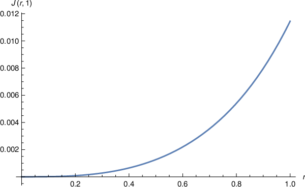
If , the integrals , and can be easily evaluated numerically.1515 15 The simplest way is to use the Mathematica numerical integration routine to integrate over the domain , , , imposing the conditions and but we have also evaluated it using other methods always with the same results. It is convenient to write the complete function defined in (22), setting as with . The function is shown in Fig. 5. The complete result can be therefore written as
| (27) |
It is, however better to express it in terms of , where - the Fermi wave vector in the case , which does not change when the ratio (i.e. the system’s polarization) is varied. Since ,
| (28) |
This energy density is plotted in Fig. 6 as a function of the system’s polarization (; it is related to the variable by ) for five different values of the expansion parameter . We have checked that our result agrees with that of [19].1616 16 The precise relation, checked numerically, of the function used in [19] (the variable used there is our polarization ) to the function defined by (22) evaluated with the cutoff and is The computed correction of order is rather small, % for and and decreases with decreasing . All curves assume at the same value - due to the Pauli exclusion principle interactions do not induce any corrections to the ground state of a fully polarized (, ) system of fermions.1717 17 This readily follows from the form of the effective iteraction written in terms of the field operators , introduced in (19) and the absence of the “sea” of oppositely polarized fermions; the same can be also inferred by writing explicitly the original interation Hamiltonian (2) in terms of creation and annihilation operators associated with different spin projections. Note also that the prefactor in (28) can be written in the form . Therefore, our Fig. 6 can be directly compared to Fig. 3 of ref. [20]: our curve for corresponds to the lowest curve in this plot obtained for a model repulsive potential by a numerical estimate of the exact ground state energy. It is seen that the result of the second order expansion is somewhat lower than the numerical estimate. This agrees with the comparison of the ground state energies of the unpolarized system (, ) performed in Fig. 2 of ref. [20] which shows that the perturbative expansion of the ground state energy in powers of remains reliable up to but is systematically below the numerical estimates of the exact value.

5 Summary
We have recomputed the order , where is the -wave scattering length and , correction to the ground state energy of a polarized gas of (nonrelativistic) fermions of spin using the effective theory approach proposed in [2] which does not require specifying explicitly the (spin independent) interaction potential. We have demonstrated the cancellation of ultraviolet divergences when the result is expressed in terms of the scattering length. Our result obtained by the method applicable to arbitrary repulsive interaction potentials is identical with that of [19] obtained with the help of traditional methods within the specific model of hard spheres. That it should be so is almost obvious in the effective theory approach but wasn’t such in the old framework.
Since the main technical problem of this approach is only isolating ultraviolet divergences and working out cancellation of imaginary contributions, it seems that with some more labour the computations presented here could be extended to yet higher orders of the expansion, similarly as was done in the case of unpolarized system in [2] and [13]. A more challenging task would be obtaining a rigorous estimate of the high order terms of the perturbative expansion which could allow to assess the range of its convergence.
In this paper we have considered the polarized diluted gas of (nonrelativistic) interacting spin fermions, working in the continuum version of the theory. Our results can be most naturally applied to atomic gases bound in traps. An analogous problem can of course be also formulated using the lattice version, that is within the paradigmatic Hubbard model, with obvious applications to atomic gases bound in periodic laser traps and to the solid state systems. As far as we know, there are no second order results similar to ours in this other version (rigorous first order results have been given in [26] and [30]) and it would be interesting to try to obtain them.
Acknowledgments. We would like to thank Pierbiagio Pieri for bringing reference [19] to our attention.
References
- [1] see e.g. Proceedings of the Joint Caltech/INT Workshop Nuclear Physics with Effective Field Theory, ed. R. Seki, U. van Kolck and M. Savage (World Scientific, 1998); Proceedings of the INT Workshop Nuclear Physics with Effective Field Theory II, ed. P.F. Bedaque, M. Savage, R. Seki and U. van Kolck (World Scientific, 2000).
- [2] H.-W. Hammer, R. J. Furnstahl, Nucl. Phys. A 678, 277 (2000); arXiv:nucl-th/0004043.
- [3] J.V. Steele, arXiv:nucl-th /0010066v2.
- [4] R. J. Furnstahl, H.-W. Hammer and N. Tirfessa, Nucl. Phys. A 689, 846 (2001).
- [5] R.J. Furnstahl and H.-W. Hammer, Phys. Lett. B 531, 203 (2002).
- [6] A. L. Fetter and J. D. Walecka, Quantum Theory of Many Particle Systems. McGraw Hill, 1971.
- [7] W. Lenz, Z. Phys. 56, 778 (1929).
- [8] K. Huang and C. N. Yang, Phys. Rev. 105, 767 (1957).
- [9] C. de Dominicis and P.C. Martin, Phys. Rev. 105, 1417 (1957).
- [10] G. A. Baker, Phys. Rev. 140, 9 (1965).
- [11] V. N. Efimov, Sov. Phys. JETP 22, 135 (1966).
- [12] M. Y. Amusia and V. N. Efimov, Ann. Phys. 47, 377 (1968).
- [13] C. Wellenhofer, C. Drischler and A. Schwenk, Phys. Lett. B 802 (2020) 135247.
- [14] N. Kaiser, Nucl. Phys. A860, 41 (2011), Eur. Phys. J. A48, 148 (2012), A53, 104 (2017).
- [15] G.-B. Jo et al., Science 325 (2009) 1521.
- [16] D. Vollhardt, N. Blümer, K. Held and M. Kollar, Metallic Ferromagnetism - An Electronic Correlation Phenomenon. In: Band-Ferromagnetism. Ground-State and Finite-Temperature Phenomena, Edited by K. Baberschke, M. Donath, W. Nolting, Lecture Notes in Physics, vol. 580, p.191 (2001).
- [17] E. H. Lieb, R. Seiringer and J. P. Solovej: Phys. Rev. A71, 053605 (2005).
- [18] M. Falconi, E. L. Giacomelli, Ch. Hainzl and M. Porta, arXiv:2006/00491[math-ph].
- [19] S. Kanno, Prog. Theor. Phys. 44, 813 (1970).
- [20] S. Pilati, G. Bertaina, S. Giorgini and M. Troyer, Phys. Rev. Lett. 105, 030405 (2010), arXiv:1004/1169 [cond-mat.quant-gas].
- [21] S. Pilati, I. Zintchenko and M. Troyer, Phys. Rev. Lett. 112, 015301 (2014), arXiv:1308/1672 [cond-mat.quant-gas].
- [22] R.P. Feynman, Statistical Mechanics. A Set of Lectures, W.A. Benjamin, Inc. 1972.
- [23] L.G. Molinari, ArXiv:1710.09248 [math-phys].
- [24] T. Schäfer, C.-W. Kao and S.R. Cotanch, Nucl. Phys. A 762 82 (2005).
- [25] H.-W. Hammer and S. König, Lect. Notes Phys. 936 93 (2017).
- [26] A. Giuliani, J. Math. Phys. 48, 023302 (2007); math-ph/0611034.
- [27] P.H. Chankowski, A. Lewandowski, K.A.M. Meissner and H. Nicolai, Mod. Phys. Lett. A30 (2015) 02, 1550006; P.H. Chankowski, A. Lewandowski and K.A.M. Meissner, JHEP 11 (2016) 105.
- [28] see e.g. L.D. Landau and E.M. Lifshitz, Nonrelativistic Quantum Mechanics, par. 137.
- [29] S. Weinberg, The Quantum Theory of Fields, Vol. I, The Press Syndicate of the University of Cambridge, 1995.
- [30] R. Seiringer, J. Yin, J. Stat. Phys. 131, 1139.