Analytical considerations for optimal axion haloscope design
Abstract
The cavity haloscope provides a highly sensitive method to search for dark matter axions in the microwave regime. Experimental attempts to enhance the sensitivity have focused on improving major aspects, such as producing strong magnetic fields, increasing cavity quality factors, and achieving lowest possible noise temperatures. Minor details, however, also need to be carefully considered in realistic experimental designs. They are associated with non-uniform magnetic fields over the detection volume, noise propagation under attenuation and temperature gradients, and thermal disequilibrium in the cavity system. We take analytical approaches to these topics and offer optimal treatments for improved performance.
August 11, 2026
Keywords: axion haloscope, non-uniform magnetic field, noise propagation, hot rod issue
1 Introduction
The axion is a hypothetical elementary particle resulting from the Peccei-Quinn mechanism proposed to solve the strong CP problem in particle physics [1, 2]. The invisible axions with a small mass may have pervaded the early universe in a stable state [3] and thus their relic abundance could provide a clue to the mysterious dark matter halo in our galaxy at the present time [4]. This pseudoscalar boson is regarded to be perceivable as a form of microwave photon to which it converts under a strong magnetic field [5]. The cavity-based haloscope is the most sensitive and efficient experimental method to use when searching for dark matter axions as it detects the resonant signal power, which can be formulated as [6]
| (1) |
where is the axion-photon coupling, and are the mass and local density of the dark matter axion, is the angular frequency of the cavity mode under consideration, is the average of the square of the externally applied magnetic field inside the cavity volume , and and are quality factors of the cavity and axion, respectively. The form factor represents the geometric alignment of the cavity mode with the externally applied magnetic field and is given by
| (2) |
where is the axion-induced electric field associated with the resonant mode and is the relative permittivity within the volume.
Since the mass of the axion is not predictable, the experiment must be capable of tuning the resonant frequency. The performance of an experiment is characterized by the frequency scan speed with a given sensitivity, which is obtained with the radiometer equation [7] using the Boltzmann constant , as follows:
| (3) |
Here, SNR is the desired signal-to-noise ratio. The system noise, represented by the equivalent temperature , is determined from the linear sum of the thermal noise from the cavity and the added noise by the receiver chain, where the latter contribution is predominated by the noise of the first stage amplifier. The search frequency is tuned by altering the electromagnetic field of the cavity mode, typically by employing a tuning structure inside the cavity.
Major experimental efforts to improve the scan speed have been made for the key elements [8] – high-field magnets [9] and large-volume high-quality cavities [10] for signal enhancement, and low-temperature refrigerators and quantum-noise limited amplifiers [11, 12, 13] for noise reduction. However, minor ingredients also influence the signal and noise estimation, and thus have non-trivial effects on experimental performance. They include non-uniformity of the applied magnetic field, noise development by lossy transmission lines with a temperature gradient, and thermal disequilibrium between the cavity and the tuning structure. These factors have been implicitly considered or partially addressed, but not explicitly discussed or fully addressed. Herein, we review these topics in an analytical manner to examine the potential effects and provide optimal treatments for sensitivity improvement.
2 Non-uniform magnetic fields
The form factor, expressed here by Eq. 2, is estimated based on a simulation and obtained in a straightforward manner under an uniform magnetic field. In reality, however, the magnetic field of a solenoid with a finite length is not uniform over the magnet bore and gradually decreases along the main axis with the development of stray field in the radial direction. Therefore, a reasonable estimation of requires knowledge of the overall field distribution within the cavity volume.
As long as a magnetic field is present in space, the axion-to-photon conversions would take place and hence a longer cavity, which stores more of the magnetic field, would be beneficial. However, Eqs. 1 and 2 indicate that the conversion power is proportional to , which eventually decreases with an increase in the cavity volume under a decreasing magnetic field. This occurs because the energy density of axion-induced photons would not remain the same for a volume-varying cavity under a non-uniform magnetic field. This effect can also be understood by approximating a single long cylindrical cavity under a non-uniform solenoid magnetic field to a series of disc-shaped cavities, each of which is under a uniform field with a different strength, coupled to a common signal combiner, such that increasing the cavity volume (length) is equivalent to adding more discs, as shown in Fig. 1. The individual disc cavities would generate different levels of signal power depending on the field strength. Noting the fact that unbalanced inputs to a power combiner induce power dissipation, the combined power would be lower than a simple sum of the input powers [14]. In other words, a continuous increase of the cavity volume under a finite magnetic field would not always be beneficial.

This intuition indicates that the cavity length can be optimized for a given magnetic field distribution to maximize the scan speed, equivalently , a product of the experimental parameters in Eq. 3 with the limit of . For a cylindrical cavity, the quality factor is given by
| (4) |
where and are correspondingly the cavity radius and length and is the skin depth of the cavity surface. For the TM010 mode, Eq. 2 can be expressed in the two-dimensional cylindrical coordinate system () as
| (5) |
where is a -th Bessel function of the first kind, is the first root of , and is the external magnetic field scaled by the field strength at the magnet center . For a uniform magnetic field, , and the from factor reaches its maximum value of . Eqs. 4 and 5 provide an expression of the scan speed in terms of the geometric parameters and functions, as
| (6) |
The integral part in Eq. 6 can be replaced by a series expansion of a known magnetic field profile at , , which yields an analytically resolvable form
| (7) |
where is the coefficient of the series expansion (see Appendix A for the derivation).

In practice, the magnetic field profile is available either from the manufacturer or by measurements, and the optimal cavity length can be obtained using Eq. 7. An example is given by a cavity experiment reported in Ref. [15], where a 9T/127mm superconducting (SC) magnet was utilized. Using the field profile provided by the manufacturer, Eq. 7 is solved as a function of the cavity length, as shown in Fig. 2. The analytical calculation is in very good agreement with a simulation result based on the finite element method. The optimal cavity length is found at the maximum value of the scan speed by requiring . It is noted that uniform magnetic fields yield considerable high scan speeds particularly for large cavity lengths, which could lead to an overestimation of the experimental sensitivity.
The optimal length of a cylindrical cavity, in general, depends on the relative dimension of the given magnet, typically represented by the aspect ratio , where and are correspondingly the magnet height and the bore diameter. The dependency obtained based on Eq. 7 is presented in Fig. 3, where the overall behavior is verified by numerical calculations for various values of . Some interesting features are noticed: 1) the optimal cavity length is always larger than the magnet height; and 2) it converges to the magnet height for large values of while approaching the bore size for small values. This provides a guideline for the cavity design for a given magnet.

3 Noise propagation
One of the intricate tasks in axion experiments is to estimate the system noise, particularly the added noise caused by the receiver chain, with high accuracy. This is true because a typical cryogenic cooling system consists of multiple stages with RF components mounted, making it complicated to understand how the noise propagates between components at different temperatures. The RF signal and noise go through attenuation as well as a temperature change while propagating through the components. These effects influence the accuracy of the relevant measurements and thus need to be properly understood.
A non-zero temperature generates thermal noise power of over bandwidth [16]. When thermal noise propagates between two different physical temperatures, from to , through a passive component with attenuation , the noise power at the final stage is given by the Johnson-Nyquist formula as
| (8) | ||||
Eq. 8 reads that the resistor generates the same amount of noise as that attenuated by itself according to the law of conservation of energy. The variable in the square brackets is defined as the equivalent noise temperature,
| (9) |
which satisfies when .
For general components, RF propagation is associated with gradual attenuation and temperature variations. A good example is a lossy transmission line connecting two different stages of a cooling system. Such a component can be approximated as a continuum of identical small segments, each of which has constant attenuation and constant temperature variation , such that and . The noise temperature at the -th segment is then given by
At the limit of , Eq. 9 can be reformulated to
| (10) |
which describes noise propagation in a more realistic sense (see Appendix B for the derivation). Figure 4 shows the dependence of the propagated noise temperature on the difference between the initial and final physical temperatures for various values of attenuation. The effective noise is elevated by a positive temperature gradient while being depressed by attenuation.

The effects of the temperature gradient and attenuation on the noise propagation must be carefully taken into account for an accurate estimation of the system noise. For cavity haloscope experiments, there are two circumstances where such effects would matter. First, noise measurements typically rely on the responses of the device under test (DUT) to its inputs. For instance, for the Y-factor method, a noise source feeds the thermal noise equivalent to two different temperatures through a non-lossless RF line into the DUT, whose temperature is held constant during the measurements. Second, the thermal noise generated from a detection cavity undergoes attenuation by a transmission line before the first stage of the receiver chain, which can be placed at a different temperature. We use Eq. 10 to treat the noise propagation appropriately and to estimate the noise temperatures in realistic conditions.
3.1 Y-factor method
The Y-factor method, a popular technique for an accurate measurement of the noise figure of a DUT, is widely adopted in axion search experiments to estimate the gain and noise temperature of an amplifier or an entire receiver chain [17]. This method evaluates the intrinsic noise of the DUT based on the ratio of the output powers to the input thermal noise powers corresponding to two different known temperatures. The noise source could be a diode which has a pre-calibrated excess noise ratio (ENR) or a resistor whose temperature can be controlled by a heater [18].
If the output noise powers through the DUT for two different (cold and hot) source temperatures, and , are denoted by and , respectively, the noise temperature of the DUT itself can be obtained using the following well-known equations:
| (11) |
However, in reality, the thermal noise from the source undergoes attenuation and a temperature gradient while propagating through a transmission line to the input of the DUT. This effect can be reflected by replacing with in Eq. 11; i.e.,
| (12) |
where obeys Eq. 10. For a noise source initially in a thermal equilibrium with the DUT, holds, as can be verified by Eq. 10.
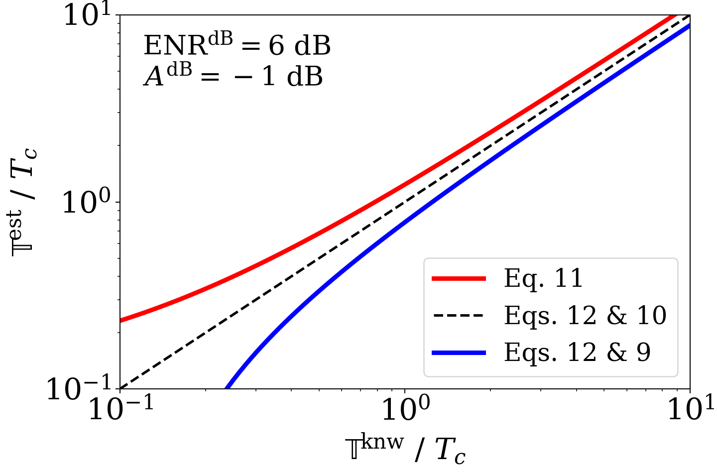
Figure 5 exhibits the effect of the noise propagation on the noise estimation using the Y-factor method. Without consideration of the effect, equivalent to Eq. 11, the Y-factor method overestimates the noise of the DUT, as represented by the red line. The effect would be manifested when a DUT is placed at a cryogenic temperature while a noise diode is placed at room temperature as such a configuration would typically add more attenuation and a higher temperature gradient. On the other hand, if the attenuation is not properly considered, e.g., if it is described by a single-step function as Eq. 9, the Y-factor method yields underestimated noise figures, as represented by the blue line. It is also noted that the discrepancies are greater for DUTs with lower noise levels. Therefore, the noise propagation must be carefully considered when estimating the noise properties of the receiver chain in a complicated system.
3.2 Cavity thermal noise
In axion haloscopes, the total noise of the system is evaluated as the thermal noise generated by the cavity transmitted through a RF line to the receiver chain, where the shot noise of electronics is linearly added while propagating through the chain. From the argument developed in this section, the noise propagation effects must be reflected when estimating the noise temperature of the system such that
| (13) |
where is the equivalent temperature of the thermal noise traveling from the cavity to the first-stage amplifier, obtained using Eq. 10, while is the added noise temperature stemming from the receiver chain, obtained from Eq. 12.
In a more practical haloscope design, additional RF components could be introduced between the detection cavity and the receiver chain for multiple purposes. A typical example is a RF circulator, which serves to circumvent the impedance mismatching effect and/or to measure the cavity properties. As illustrated in Fig. 6a, it could be placed at a different temperature. To maximize the scan speed, the signal pickup antenna is configured to over-couple to the cavity [6], conventionally represented by , where is the coupling strength. In such a configuration, not only the signal but also the noise is subjected to reflection due to the impedance mismatch between the antenna and the cavity. This complicates the noise propagation, which is described as
| (14) |
where ′ represents direct propagation of the noise originating from the cavity to the receiver, while ′′ represents the back-and-forth propagation of the noise coming from the circulator, reflected by the cavity, and going to the receiver. Eq. 14 can be used to estimate the noise temperature from the perspective of the receiver (the first-stage amplifier), depending on the physical temperature of the amplifier relative to that of the cavity. Figure 6b gives an example of such a dependency in the presence of a circulator between the two components for various values of the line attenuation. It would be beneficial to maintain the physical temperature of the amplifier lower than that of the cavity.


4 Hot rod problem
It was reported in an axion haloscope experiment that the noise power near the cavity resonant frequency was significantly higher than the noise power observed off resonance [12]. It turns out that the excess noise on resonance was attributed to poor thermalization of the frequency tuner (a conducting rod) located inside the cavity. Known as the hot rod problem, the issue was addressed to some extent by improving the thermal link to the tuner at the cost of a reduction of the cavity quality factor [13]. As such an issue could be common in haloscope experiments, it should be carefully considered when designing an experiment. Here we analytically estimate the effect of the thermal disequilibrium between the cavity and the frequency tuner on the overall thermal noise.
Many axion experiments are conducted at very low temperatures due to the advanced cryogenic technologies, necessitating consideration of the quantum effects in thermal noise. In this regard, we define the effective temperature as follows:
| (15) |
Here, is the reduced Planck constant. The first term of Eq. 15 represents the average thermal photon number at physical temperature at frequency , while the second term accounts for zero-point fluctuations, reflecting the quantum limit near absolute zero.
For a cavity with a tuning structure inserted, the thermal temperature observed by the antenna coupled to the cavity can be decomposed into two components:
where are the effective temperatures of the cavity and the tuning structure, with representing their fractional contributions. Given that, as previously mentioned, passive devices generate noise to the extent of their dissipation, the fractions can be written as
| (16) |
where , satisfying , are the dissipated power by the corresponding objects. Depending on the material, the power dissipation formulae for an arbitrary resonant mode with electromagnetic fields of and are given by
| (17) |
where the subscripts and denote the dielectrics and conductors. For the former, the power dissipation is associated with the dielectric loss within its volume, while for the latter, it depends on the surface resistance (with conductivity ) over its surface area.
Equation 17 can be explicitly solved for a certain configuration, for instance, a long cylindrical cavity of radius with a cylindrical conducting rod of radius positioned at the center of the cavity. The dissipated power by the cavity and rod is proportional to and , respectively, and Eq. 16 simply becomes
| (18) |
which is verified using the field profiles obtained from simulations with various rod radii. The fractional contributions from the tuning rods of two different materials are shown in Fig. 7a as a function of the relative rod size . Figure 7b exhibits the dependence of the noise contribution on the rod position with respect to the center of the cavity; the closer to the cavity center it is, the larger the contribution it makes. Figure 8 provides an example showing how the observed effective temperature would develop with different rod temperatures assuming a configuration identical to that in Fig. 7a with . Because, depending on detector design, the noise contribution by a tuner can be substantial, especially for a conductor, it would be essential to establish a good thermal link to it.


5 Conclusion
In this report, we considered some minor issues to be addressed in axion haloscope experiments. We explicitly analyzed their influences on signal and noise estimation, based on which we suggest optimal designs to improve search performance. Non-uniformities in external magnetic fields limits the energy density of axion-induced photons for a given cavity, and an optimal length was found to maximize the signal power. The noise propagation was practically evaluated under temperature gradient and RF attenuation conditions to derive appropriate treatments for noise estimations using the Y-factor method and noise development with additional components. In addition, the hot rod problem was revisited to provide an analytical method by which to calculate the effects of thermal disequilibrium between a cavity and a frequency tuner. These effects need to be carefully taken into account when designing or conducting an experiment, as they will have non-trivial effects on experimental sensitivity.
Acknowledgement
This work was supported by the Institute for Basic Science (IBS-R017-D1-2021-a00).
Appendix A Series expansion of the form factor
The electric field solution for the TM010 mode of a cylindrical cavity with radius is given in the cylindrical coordinates with time by
where is the mode amplitude, is the resonant frequency of the mode, is the zeroth Bessel function of the first kind and is its first root. Using this solution, Eq. 2 can be transformed to
| (19) |
where is the scaled magnetic field, which becomes for an uniform magnetic field. Equation 19 expresses the form factor as a distribution function of . Employing the Ampere’s law in vacuum and the divergence-free condition of the applied magnetic field, we can expand in power series of the field profile along the solenoid axis, , as
The integral part in Eq. 19 becomes
where represents the average value over the cavity length for the relevant quantity. The coefficient is obtained from a volume integral of the Bessel function in Eq. 19 as follows
where is a generalized hypergeometric function [19].
Appendix B General equation for noise propagation
In axion haloscopes, signal and noise go through power loss and temperature difference through a series of RF components at different stages. To a first approximation, a typical RF component has gradually varying attenuation and temperature, and thus they can be depicted as a continuum of identical small segments, -th of which has infinitesimal attenuation and temperature variation , such that
| (20) |
Applying Eq. 9, the noise temperature at the -th segment, , is given by
| (21) |
which must be distinct from the physical temperature . If we assume constant attenuation and temperature gradient for all segments, i.e., and for all , then Eq. 21 becomes
| (22) |
This assumption would reasonably hold particularly for commercial RF transmission cables connecting two different temperature stages.
Solving the recurrence relation Eq. 22 for infinite with the initial condition of , we obtain
which eventually yields an expression for the total noise temperature
| (23) |
in terms of the known total attenuation and temperature variation . For the initial condition of , the solution for Eq. 22 returns Eq. 10
| (24) |
which provides a general description of noise propagation through a continuum with constantly varying attenuation and temperature. In the limits of , e.g., for a nearly lossless component, Eq. 24 is simplified to
| (25) |
Eq. 24 can be further generalized for a RF system with attenuation and temperature arbitrarily distributed over the body. This can be described by the same approximation as Eq. 20 assuming and are fixed within a single segment but varying segment by segment. Eq. 24 itself describes the noise propagation within a single segment, while iteration of it develops the noise temperature with increasing segment number as follows
| (26) |
where the subscript represents noise propagation from node to node . In the limit of , the continuum of a series of segments can be treated as a continuous object and then Eq. 26 is rewritten in integral form of
| (27) |
where is the temperature (attenuation) at (up to) distance from the initial point. Eq. 27 corresponds to the most general equation of noise propagation through a RF system with arbitrarily distributed temperature and attenuation, providing an exact estimation of noise temperature for known functions of and .
References
- [1] R.D. Peccei and H.R. Quinn, CP Conservation in the Presence of Pseudoparticles, Phys. Rev. Lett. 38, 1440 (1977); R.D. Peccei and H.R. Quinn, Constraints imposed by CP conservation in the presence of pseudoparticles, Phys. Rev. D 16, 1791 (1977).
- [2] S. Weinberg, A new light boson?, Phys. Rev. Lett. 40, 223 (1978); F. Wilczek, Problem of strong P and T invariance in the presence of instantons, Phys. Rev. Lett. 40, 279 (1978).
- [3] J. E. Kim, Weak-interaction singlet and strong CP invariance, Phys. Rev. Lett. 43, 103 (1979).
- [4] J. Preskill, M. B. Wise and F. Wilczek, Cosmology of the invisible axion, Phys. Lett. B 120, 127 (1983); L. F. Abbott and P. Sikivie, A cosmological bound on the invisible axion, Phys. Lett. B 120, 133 (1983); M. Dine and W. Fischler, The not-so-harmless axion, Phys. Lett. B 120, 137 (1983).
- [5] P. Sikivie, Experimental Tests of the ”Invisible” Axion, Phys. Rev. Lett. 51, 1415 (1983).
- [6] D. Kim et al., Revisiting the detection rate for axion haloscopes, J. Cosmol. Astropart Phys. 03, 066 (2020).
- [7] R.H. Dicke, The Measurement of Thermal Radiation at Microwave Frequencies, Rev. Sci. Instrum. 17, 268 (1946).
- [8] R. Bradley et al., Microwave cavity searches for dark-matter axions, Rev. Mod. Phys. 75, 777 (2003); Y. K. Semertzidis and S.W. Youn, Axion Dark Matter: How to detect it?, arXiv preprint, arXiv:5104.14831 (2021).
- [9] R. Gupta et al., Status of the 25 T, 100 mm Bore HTS Solenoid for an Axion Dark Matter Search Experiment, IEEE Trans. Appl. Supercond. 29, 5 (2019).
- [10] D. Alesini et al., Galactic axions search with a superconducting resonant cavity, Phys. Rev. D 99, 101101 (2019); D. Ahn et al., First prototype of a biaxially textured YBa2Cu3O7-x microwave cavity in a high magnetic field for dark matter axion search, arXiv preprint, arXiv:2103.14515 (2021).
- [11] S.J. Asztalos et al., SQUID-Based Microwave Cavity Search for Dark-Matter Axions, Phys. Rev. Lett. 104, 041301 (2010); T. Braine et al., Extended Search for the Invisible Axion with the Axion Dark Matter Experiment, Phys. Rev. Lett. 124, 101303 (2020); K.M. Backes et al., A quantum enhanced search for dark matter axions, Nature 590, 238 (2021); C. Kutlu et al., Characterization of a flux-driven Josephson parametric amplifier with near quantum-limited added noise for axion search experiments, arXiv preprint, arXiv:2104.08496 (2021).
- [12] B.M. Brubaker et al., First Results from a Microwave Cavity Axion Search at 24 eV, Phys. Rev. Lett. 118, 061302 (2017);
- [13] L. Zhong et al., Results from phase 1 of the HAYSTAC microwave cavity axion experiment, Phys. Rev. D 97, 092001 (2018).
- [14] D.S. Kinion, First results from a multiple-microwave-cavity search for dark-matter axions, University of California, Davis (2001); H. Hausman, Understanding mismatch effects in power combining circuits, Microwaves & RF 45 (2006).
- [15] J. Jeong et al., Search for Invisible Axion Dark Matter with a Multiple-Cell Haloscope, Phys. Rev. Lett. 125, 221302 (2020).
- [16] J.B. Johnson, Thermal agitation of electricity in conductors, Phys. Rev. 32 97 (1928); H. Nyquist, Thermal agitation of electric charge in conductors, Phys. Rev. 32 110 (1928).
- [17] Keysight Technologies, Application Note 5952-3706E (2019). https://www.keysight.com/kr/ko/assets/7018-06829/application-notes/5952-3706.pdf
- [18] S.W. Youn et al., Noise temperature measurements for Axion haloscope experiments at IBS/CAPP, J. Low Temp. Phys. 200, 472 (2020).
- [19] B. Dwork, Generalized hypergeometric functions, Oxford University Press on Demand (1990).