A Machine Learning-based Direction-of-origin Filter for the Identification of Radio Frequency Interference in the Search for TechnosignaturesJournal: Astronomical JournalTensorFlow (Abadi et al. 2015), NumPy (Harris et al. 2020), SciPy (Virtanen et al. 2020), scikit-learn (Pedregosa et al. 2011), pandas (Wes McKinney 2010), Matplotlib (Hunter 2007)
Abstract
Radio frequency interference (RFI) mitigation remains a major challenge in the search for radio technosignatures. Typical mitigation strategies include a direction-of-origin (DoO) filter, where a signal is classified as RFI if it is detected in multiple directions on the sky. These classifications generally rely on estimates of signal properties, such as frequency and frequency drift rate. Convolutional neural networks (CNNs) offer a promising complement to existing filters because they can be trained to analyze dynamic spectra directly, instead of relying on inferred signal properties. In this work, we compiled several data sets consisting of labeled pairs of images of dynamic spectra, and we designed and trained a CNN that can determine whether or not a signal detected in one scan is also present in another scan. This CNN-based DoO filter outperforms both a baseline 2D correlation model as well as existing DoO filters over a range of metrics, with precision and recall values of 99.15% and 97.81%, respectively. We found that the CNN reduces the number of signals requiring visual inspection after the application of traditional DoO filters by a factor of 6–16 in nominal situations.
Keywords:
Search for extraterrestrial intelligence — technosignatures — astrobiology — radio astronomy — Convolutional neural networksI Introduction
Radio technosignature searches have increased dramatically both in scope and complexity since the early days of the search for extraterrestrial intelligence (Drake 1965; Tarter 2001; Tarter et al. 2010; Drake 2011, and references therein). In the past three years alone, the UCLA SETI Group’s radio technosignature detection algorithms have undergone multiple levels of improvements, increasing the total number of detections in a typical 2-hour observing window by more than an order of magnitude (Pinchuk et al. 2019; Margot et al. 2021). Our current pipeline detects 200 times more signals per unit bandwidth per unit integration time than recent Breakthrough Listen (BL) searches (Enriquez et al. 2017; Price et al. 2020; Gajjar et al. 2021) with the same telescope, receiver, and detection threshold. We have also improved our radio frequency interference (RFI) excision algorithms, yielding RFI classification accuracies of on data sets with millions of candidate signals. Other groups are making progress along these lines as well. For instance, the custom hardware system that enabled the early 1990s NASA High Resolution Microwave Survey was migrated to a software platform whose RFI excision capabilities have continued to evolve (Harp et al. 2016). Traas et al. 2021 reported the results from a search of 28 targets selected from the TESS Input Catalog and also described an improvement to the BL RFI excision technique.
Despite these advancements, RFI remains the biggest challenge to the search for technosignatures. Pinchuk et al. 2019 and Margot et al. 2021 described several pitfalls of current RFI identification algorithms that rely on inferred signal properties, such as estimates of frequency and frequency drift rate. They suggested that these hurdles might be overcome by an algorithm that instead examines the structure of candidate signals in time-frequency space. Because the time-frequency structure of a signal resembles an image, we can readily apply modern computer vision techniques to this problem, as also suggested by Cox et al. 2018, Zhang et al. 2018, Harp et al. 2019, and Brzycki et al. 2020.
The last decade (2010-2020) has seen considerable advances in the field of Convolutional Neural Networks (CNNs). In 2012, Krizhevsky et al. 2012 introduced the AlexNet architecture, which won the ImageNet ILSVRC challenge (Russakovsky et al. 2015) the same year. This architecture achieved a top-five error rate of , which represents the percentage of test images (256256 pixels) for which the network’s top five predictions, chosen from a total of 1000 classes, did not include the correct answer. This was an unprecedented accomplishment at the time. An explosion of CNN architectures followed in subsequent years, each performing better than the last (Simonyan & Zisserman 2014; Szegedy et al. 2015; He et al. 2016; Chollet 2017). Modern CNN architectures have achieved top-five error rates of or less (Tan & Le 2019, e.g.,).
Machine learning (ML) has permeated both the workforce and the research industry, often leading to large improvements in challenging classification problems. In particular, astronomers have already applied CNNs to push the boundaries of astronomical data analysis. For example, Schawinski et al. 2017 trained a Generative Adversarial Network composed of two CNNs (one to classify samples and another to generate them during training) to recover features such as galaxy morphology from low signal-to-noise ratio (S/N) and low angular resolution images. Shallue & Vanderburg 2018 trained a deep CNN to predict whether a signal found in Kepler data was a transiting exoplanet or a false positive, allowing them to detect and validate a five–planet resonant chain around Kepler–80 and a new, eighth planet around Kepler–90. Zhang et al. 2018 detected 72 new pulses from the repeating fast radio burst FRB 121102 using a CNN trained on radio astronomy data obtained with the Green Bank Telescope. For a more detailed overview of ML and CNNs applied to astronomy, see Baron 2019 and references therein.
CNN applications have been explored in the context of radio technosignature searches. Cox et al. 2018 and Harp et al. 2019 both generated a labeled set of synthetic candidate signals from a small () number of RFI classes to train a CNN for RFI classification. Although this approach provides a relatively simple way to obtain a labeled training set, the synthetic signals may not be representative enough of actual signals and may therefore introduce a bias during model training. Zhang et al. 2018 avoided this problem by using self-supervised learning to train their network. Specifically, their CNN was trained to predict the future time-frequency structure of a signal given the time-frequency structure from a past subset of the total observation. This method allowed the observations to act as both the training set and the training labels for the model. However, in order to apply the network for RFI excision, the similarity of the predicted signals and the observed signals must be evaluated. Because this task is not trivial, the RFI classification performance of the network may suffer. Brzycki et al. 2020 explored the application of CNNs to technosignature candidate signal detection. Specifically, the authors trained a CNN to detect up to two signals in a frequency span of 1400 Hz. Although a potential improvement over the detection algorithms of Enriquez et al. 2017 and Price et al. 2020, this CNN cannot yet compete with the detection algorithms described by Margot et al. 2021, which can detect hundreds of signals within the same frequency range.
In this work, we describe an application of CNNs to the excision of RFI in technosignature data. The article is organized as follows. Our motivation and approach to this problem are presented in Section II. Our data compilation procedure is detailed in Section III. In Section IV, we describe our approach to CNN model selection and hyperparameter tuning. We also describe a non-ML baseline model that we use as a point of comparison to the trained CNN. Section V summarizes our results, including the final model performance on the test set as well as on archival data. In Section VI, we describe several failure modes of our trained network and offer avenues for future improvements. We present conclusions in Section VII.
II Motivation and Approach
Modern radio technosignature programs detect millions of signals per survey (Siemion et al. 2013; Harp et al. 2016; Enriquez et al. 2017; Margot et al. 2018; Pinchuk et al. 2019; Price et al. 2020; Margot et al. 2021; Gajjar et al. 2021, e.g.,). These signals must be carefully analyzed to determine whether or not they are of anthropogenic nature. The standard approach to perform this analysis is the direction-of-origin (DoO) filter. This filter labels a signal as RFI if it is not persistent in one direction on the sky or if it is detected in multiple directions on the sky. Theoretically, this filter is powerful enough to remove all RFI signals that are detected in multiple scans. In practice, this filter often fails on a small subset of signals, but even failure rates as low as can be costly because visual inspection of the remaining signals may be necessary. For instance, the filter failure rates in the searches of Pinchuk et al. 2019 and Margot et al. 2021 were and , respectively, requiring further examination of 96,940 and 43,020 signals, respectively.
The main pitfall of the DoO filter is the accuracy with which a unique signal can be linked across multiple scans. This “signal pairing” is required for both the persistence-test (present in all scans of the source) and the uniqueness-test (absent in scans of other sources) portions of the filter. Different surveys implement this pairing functionality in various ways. For example, Enriquez et al. 2017 and Price et al. 2020 considered two signals to be from a common origin if the frequency at which the latter signal is detected is within a generous tolerance of Hz of the detection frequency of the first signal, even if the corresponding frequency drift rates are unrelated. Although this approach speeds up the analysis by discarding a large portion of the candidate signals, it is problematic because it may eliminate valid technosignatures. A more rigorous approach was adopted by Pinchuk et al. 2019 and Margot et al. 2021. In both of these searches, two signals were paired only if their frequency drift rates and frequencies extrapolated to a common epoch are within a small tolerance. More robust versions of this filter could include tests of other signal properties, such as signal bandwidth or off-axis gain ratio.
In all four searches described in the preceding paragraph, the filter was applied to estimates of signal properties produced by a computer program on the basis of the time-frequency structure of each signal. Therefore, the efficiency of the filter relies heavily on the accuracy of the derived signal properties. When the estimates of these signal properties are imprecise or incorrect, or when the underlying assumption of a linear drift rate is violated, the filter classification fails. Pinchuk et al. 2019 detailed five different signal types for which their DoO filter exhibited a degraded performance. Importantly, this limitation can likely be overcome by an algorithm that examines the time-frequency structure of each signal directly.
In this work, our approach is to train a CNN to pair signals by directly examining the corresponding dynamic spectra. The trained network is then used to examine the data as follows. For each signal detected in the survey, we extract a portion of the dynamic spectrum centered on the time-frequency location of the signal as the first input to the network. This dynamic spectrum is guaranteed to contain a signal, because the minimum detection threshold in typical SETI searches is set at ten times the standard deviation of the noise. Using an estimate of the drift rate of the signal in this dynamic spectrum, we extrapolate the expected detection frequency to the starting epoch of a different (typically subsequent) scan. We then extract a portion of the dynamic spectrum of the second scan to use as the second input to our network. This portion has the same dimensions as those of the first input and is centered on the expected detection frequency. The output of the network provides an assessment of whether or not the second dynamic spectrum contains the same signal as the first dynamic spectrum. The CNN will be trained to perform this task with a large (1 million) labeled training set, such that the CNN can make this assessment by recognizing patterns in the images, as opposed to calculating and comparing estimates of signal properties like frequency and drift rate.
In what follows, we will use the terms “first” or “top” image to refer to the dynamic spectrum of the first scan, which must contain a signal of interest. Likewise, we will use the terms “second” or “bottom” image to refer to the dynamic spectrum of the second scan, which may or may not contain the same signal.
III Data Preparation
III.1 Observations
We compiled our data set from the observations presented by Pinchuk et al. 2019. Those observations were conducted on 2017 May 4, 15:00 – 17:00 Universal time (UT) with the 100 m diameter Green Bank Telescope. Both linear polarizations of the L-band receiver were recorded with the GUPPI back end in its baseband mode (DuPlain et al. 2008). GUPPI was configured to channelize 800 MHz of recorded bandwidth into 256 channels of 3.125 MHz each.
The observations primarily consisted of sources from the Kepler field, but also included scans of TRAPPIST-1 and LHS 1140. A total of twelve sources were scanned. A full list of targets and their properties can be found in Table 1 of Pinchuk et al. 2019. This article also includes details relating to the formation of the dynamic spectra, which have a time resolution of 0.336 s and frequency resolution of 2.98 Hz.
A total of 10,293,618 signals were detected in the data, 8,592,771 of which have a S/N . Because we had a large number of signals to choose from, we carefully pruned the data according to principles described in Section III.3 in order to obtain the best possible training candidates.
III.2 Definition of Data Sets
In order to successfully train our CNN, we need to set aside several small portions of our data that we can use to evaluate the model performance during and after training. Typically, it is recommended to set aside 10–20 of the training data as a “validation” set that is used to evaluate important metrics like precision, recall, and a model cost function or loss (Géron 2019). These metrics can then be used to tune model hyperparameters (Section IV.3) or identify problems like overfitting, which occurs when a neural network simply learns to reproduce the labels of the training data and therefore generalizes poorly to any other data. Standard ML practices suggest that another 10–20 of the training data should be set aside as a “test” set that is only ever used to evaluate the performance of the final model. This evaluation is important in order to obtain an accurate estimate of how well the model generalizes to data that it has never seen before.
When the training data are representative of the data that the model will see in a production environment, the training, validation, and test sets are enough to successfully train a CNN from start to finish. However, because we needed to label a large training set in an automatic manner (Section III.4.1), our training data consist of two images taken from a single scan, whereas the production data consist of two images from entirely separate scans. This difference between training and production data makes our application atypical and requires adjustments to standard ML practices. In particular, it is possible for the network to perform well on the training data but poorly on the production data. This situation occurs when there is a “data mismatch” and often requires some manipulation of the training set in order to better match the production data. Importantly, this condition must be detected and addressed before the model is put into production. If the validation set is generated as a subset of the training set, then data mismatch is impossible to detect. On the other hand, if the validation data is comprised only of data that the model will see in production, it is not possible to discern whether poor model performance is attributable to data mismatch or to model training issues, such as overfitting, in the absence of other information. The solution to this problem is to create an additional data set, the “train–dev” set, which is a subset of 10–20 of the training data and is used to monitor the performance of the model during training and detect problems like overfitting. With the “train-dev” set on hand, we can compile validation and test sets that match the data that the model will see in production. These two data sets are hand-labeled, as is standard in most ML applications, and are therefore much smaller than the training and train–dev sets. The validation and test sets provide a useful way to select an appropriate CNN architecture, tune hyperparameters, and measure the model’s generalization to new data, among other uses.
We compiled a subset of signals from the hand-labeled validation and training sets to evaluate the performance of the UCLA SETI Group DoO filter. In order to facilitate a fair comparison to our CNN, we only kept the labeled image pairs that corresponded to different scans of the same source, and we only applied the persistence portion of the DoO filter to these signals (the signal pairing logic is identical for both components of the filter). This is important because the DoO filter examines many different scans from a single observing session to look for the presence of a given signal elsewhere on the sky. However, when determining if the signal is persistent in its detection direction, the filter only examines the two scans of the source containing the signal of interest. The latter is consistent with a standard application of the CNN trained in this work and therefore offers the best comparison between the performance of the existing DoO filter and the CNN.
We also made use of a small hand-labeled data set of image pairs to optimize and evaluate a baseline model (Section IV.1). This model, which does not rely on ML techniques, provides a mechanism to test the performance improvement due to the ML application. Table 1 summarizes the data sets utilized in this work.
| Name | Size | Usage | Hand-labeled? Production-like? |
|---|---|---|---|
| Training | 1,000,000 | Training and evaluating the CNN | No |
| Train-dev | 100,000 | Evaluating the CNN (Overfitting) | No |
| Validation | 1156 | Evaluating the CNN (Data mismatch) | Yes |
| Test | 1272 | Evaluating the CNN (Final results) | Yes |
| UCLA DoO test | 1238 | Evaluating the UCLA direction-of-origin filter | Yes |
| Baseline | 524 | Optimizing and evaluating the baseline model | Yes |
Note that the validation and test sets are much smaller than the training and train–dev sets because the former had to be analyzed and labeled by hand whereas the latter were labeled automatically, as described in Section III.4.
III.3 Data Selection Filters
We began by examining the distribution of drift rates of the 8,592,771 signals detected in 2017 (Figure 1, Left). We observed that the vast majority () of detected signals have drift rates Hz s-1.
Moreover, by examining the dynamic spectra of signals with drift rates Hz s-1, we observed a lack of the narrowband characteristics that are often chosen as one possible diagnostic of extraterrestrial engineered emitters. For these reasons, we excluded 168,684 () signals with drift rates Hz s-1 from the training set.
We performed a similar cut on the basis of the S/N of the detected signals. Instead of significantly altering the S/N distribution, however,In particular, we opted to remove any signals with extremely large S/N. Based on the cumulative distribution of S/N shown in the middle panel of Figure 1 we chose to discard any signals with a S/N . This threshold was large enough to preserve of the remaining signals but also remove any extreme S/N outliers. As a result of this filter, we removed 58,399 () signals with extreme S/N from the training set.
Next, we examined the bandwidth of the remaining signals, as quantified by a full width at half maximum (FWHM) metric. The bandwidth of the training signals is especially important because we needed our training-set signals to fit within a 225225 image. This image size was chosen to satisfy a few considerations. First, the number of linesrows cannot exceed half the number of linesrows in the dynamic spectra, which is 490 for the 2017 data at 2.98 Hz frequency resolution. Second, the number of columns must be an odd number so that signals can be perfectly centered in the image. Third, the input size for models like ResNet52 are images of size 224224 pixels (He et al. 2016) and have been shown to be manageable with modern CNN architectures. Our chosen image size corresponds to an upper limit of 670 Hz on the bandwidth of the signals. However, because we are only interested in narrowband signals ( Hz) in this work, we can set the bandwidth threshold much lower than the theoretical upper limit. The distribution shown in the right panel of Figure 1 suggests a threshold value of 100 Hz. As a result of this filter, we removed 15,044 () signals with large bandwidths from the training set.
Finally, we discarded 6447 signals that were detected close enough to the edge of their 3.125 MHz wide channel such that the signal overlapped with a neighboring channel. Although we could “stitch” neighboring channels together to fully recover these signals, given the vast number of signals left to choose from, we decided to simply remove this tiny fraction of signals from consideration for the purpose of building the training set. When we evaluate actual data with the CNN, we do combine two channels when necessary to correctly represent signals located near the channel edges.
Overall, the filters above discarded 248,594 of the 8,592,771 detected signals, leaving 8,344,177 () available to use for our training set. If we assume that the distributions of drift rates, S/N, and bandwidths remain relatively constant over time and the RFI observed with the 2017 antenna pointing directions is representative of other directions, then the network trained on our pruned data set should be applicable to 97% of the detected signals in future searches with similar parameters. If the RFI environment changes so much in time or in space that it severely alters the distributions of signal properties, this percentage value could change. Although the RFI environment may evolve in time and space, we were able to verify that these filters still captured 97% of the detected signals in searches conducted in 2018 and 2019 by Margot et al. 2021 with different antenna pointing directions. Specifically, 97.4% (9,845,561 out of 10,113,551) and 97.2% (16,048,515 out of 16,518,362) of the signals detected in 2018 and 2019, respectively, passed the data selection filters described above.
The range of signals selected for the labeled training set translates into a finite domain of applicability for the CNN. Because the CNN was not designed for signals with S/N 10, frequency drift rates Hz s-1 , or bandwidths 100 Hz, it may not perform well when applied to such signals. Therefore, we recommend eliminating signals that are outside the domain of applicability of the CNN prior to applying the CNN. Note that the applicability of the training set to new data sets and the CNN’s decision accuracy are two different concepts. We evaluate the latter in Section V.2.
III.4 Generation of the Training and Train–dev Sets
Labeling a sizable training set by hand is time-consuming. To bypass this limitation, we developed a strategy to synthetically generate our labeled data set. Because we are interested in training a neural network to supplement our DoO filters by detecting whether or a not a signal is present in two separate images, we need a training set that consists of pairs of images labeled with a binary flag indicating the persistence of a signal across both scans.
III.4.1 Creation of Image Pairs
In order to simulate a pair of scans containing the same signal, we split the image representing a single scan into two parts along the time dimension. We then evaluated whether the signal was detected in both the top and bottom parts. If the signal was detected in both, we labeled the pair as a positive sample. Otherwise, we labeled the pair as a negative sample to signify that the signal was present in only one of the two parts. In practice, the detection decisions are implemented by computing the ratio of signal powers in the top and bottom parts.
The power ratio calculations rely on the simplifying assumption that the total integrated power associated with each signal is distributed evenly throughout the duration of the scan. In other words, we expect the signal in each half of the spectrum to contribute equally to the total power. We calculated the signal power detected in each half of the scan and recorded these values as power ratios (), where the denominator is half of the total signal power in the scan. The signal power was calculated by summing pixels at each timestep along a line with a slope equal to the drift rate of the signal, where pixels on either side of the line, where is the bandwidth of the signal measured in hertz, = 2.98 Hz is the frequency resolution of the data, and is the floor operator. The drift rate of the signal was assumed to be the same in both halves of the spectrum. To calculate the signal power in the the top half of the dynamic spectrum, we started at the pixel corresponding to the detection frequency of the signal. To calculate the power of the signal in the bottom half, we started at the center frequency obtained by linearly extrapolating the signal detection frequency to the appropriate time. The total signal power was obtained by summing the two halves. By comparing the ratio of powers in the top and bottom halves of each scan to a suitable threshold, we were able to assign an appropriate label to each signal. Section III.4.2 describes the selection of the threshold.
This approach allowed us to label a large number of signals in a short period of time. We chose to compile the training and train–dev data sets from a pool of 1,100,000 total signals, which is a random selection among the 8,344,177 signals that meet certain criteria described below. For reference, the popular MNIST handwritten digit dataset (LeCun et al. 1998) as well as the CIFAR–10 (Krizhevsky 2009) multiclass image dataset both contain 60,000 samples each. Both the training and train–dev sets contain an equal ratio of positive and negative samples. We set aside 100,000 signals for the train–dev set, leaving 1 million signals to be used as the training set.
In order to be accepted into the training set or train–dev data set, signals had to satisfy several criteria. Most importantly, the top image in a pair, which mimics the first scan in an actual observing sequence, must always contain a signal. Moreover, the primary signal must always be centered in the top image and nearly centered in the bottom image, i.e., the signal must start in or near the middle of the frequency array in the topmost time bin. This requirement affects the construction and processing of the images, which are described in Section III.4.3. In particular, we allowed a small tolerance on the location of the signal in the bottom image, but the signal in the top image must always start at column 113 (if counting from 1) in the first row of the 225225 images. Both of these criteria can easily be met in production, because one can apply these cropping steps to detected signals with known starting frequencies. For signals whose bandwidth spans several pixels, the starting frequency is defined as the starting frequency reported by the detection algorithm, which is where most of the power is detected (Margot et al. 2021).
III.4.2 Selection of Suitable Signals
We began by examining the S/N of each signal in the top half of the scan only. In order to satisfy the underlying assumption that there is definitely a signal in the center of the first image (represented in the training set by the top half of the scan), we required a minimum top-half S/N of at least 6 (Figure 2), which corresponds to a 1 in a billion false detection rate.
We validated our choice of threshold by examining a sample of signals below the cutoff value. We found that most of these signals are faint and difficult to detect visually, while the rest are not present at all. On the contrary, signals above this threshold are clearly visible in the dynamic spectra. Appendix A illustrates these two cases.
As we performed our final selection, we needed to allow for variations in the S/N of the top and bottom portions of the positive signals, since the top and bottom portions represent two separate scans and we have empirically observed that the S/N can change substantially between scans. To do so, we compared the integrated power values from the top and bottom halves of each signal. Specifically, we examined the distribution of the ratio of bottom to top integrated powers (i.e., ). We found that approximately 50% of the signals have a ratio between 0.75 and 1.25 (Figure 3), so we randomly selected 550,000 signals from this region to represent our positive samples (i.e., a signal is detected in both scans/images).
Additionally, we selected 50,000 signals with a ratio of 0.2 or lower to partially represent our set of negative samples (see blue line in Figure 3). To ensure the absence of a signal from the bottom half, we verified that none of these samples had any signals with a prominence value greater than 3 times the standard deviation of the noise in the bottom half (see Margot et al. 2021, Section 3.1 for an in-depth discussion of the prominence calculation). Appendix A depicts a sample of these signals. Ideally, all negative samples would be obtained with this method, but there were not enough of these signals to provide the necessary negative samples. Since this category is grossly underrepresented in the data, we used data augmentation to create more negative samples. Specifically, the remaining 500,000 negative samples were obtained by taking samples from the region with a ratio between 0.75 and 1.25 and altering them in four different ways to remove any signals present in the bottom half. This process is described below.
III.4.3 Processing of Selected Signals
After selecting the signals for our training set, we applied some processing to ensure that signals in the positive and negative categories were representative of their respective labels.
We first considered the 550,000 signals from the positive category. When we applied our ML algorithm to real data, we obtained the bottom image by extracting a portion of the spectrum from the second scan centered on the frequency value calculated by extrapolating the frequency detected in the first scan. If the same signal is present in both scans, and if the signal’s drift in time-frequency space is approximately linear11 1 The assumption of linearity is reasonable for a source analyzed at L band with a frequency resolution of 2.98 Hz, a scan duration of 150 s, and a line-of-sight jerk below . For reference, the maximum line-of-sight jerks for Earth’s spin and orbit are and , respectively., and if the drift rate estimate is approximately correct, this method will ensure that the signal also appears in the bottom image, but it does not guarantee that the signal will be perfectly centered in the bottom image. For instance, a small discrepancy between the actual and estimated drift rates can result in an offset between predicted and actual frequency values. To simulate this scenario in our training set, we shifted all of the signals in the bottom image of our samples by 0–5 pixels (0–15 Hz). The exact shift for each image was randomly selected from a distribution of shift values described in Section IV.1.
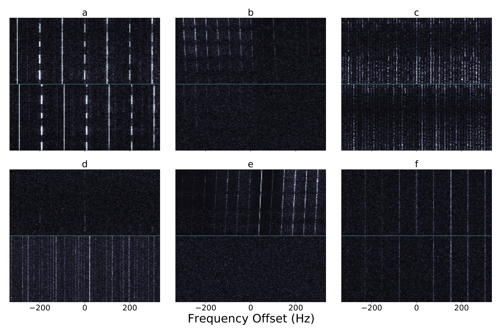
The 550,000 signals for the negative category were compiled using five distinct procedures. The first 50,000 signals were selected from the distribution shown in Figure 3 with a ratio of . For each of these signals, we verified the lack of any signals with a prominence value greater than 3 times the standard deviation of the noise in the bottom half of the scan. The next 125,000 negative samples were obtained by selecting unused signals from the “positive” range () and shifting the signal in the bottom image by 6–10 pixels (18–30 Hz). By doing so, we forced the algorithm to learn that a positive detection requires the bottom signal to be detected in close proximity to the extrapolated frequency, which is calculated on the basis of signal properties in the top image. We obtained another 125,000 negative samples by once again selecting unused signals from the “positive” range and replacing the bottom signal with an unrelated signal (also sampled from the “positive” range). This group of negative samples forced the algorithm to compare signal properties and not pair two unrelated signals that may have been detected at similar frequencies in two different scans. Another 125,000 negative samples were obtained by selecting leftover signals from the “positive” range and replacing the bottom image with noise. The noise was generated by sampling values from a distribution with four degrees of freedom that was fit to the bottom image after removing any power values belonging to any signals detected in the spectrum. The signals were removed by obtaining the database records of all signals detected within the relevant portion of the spectrum and discarding any power values within 2 times the measured bandwidth along the linear drift rate of each signal. The final 125,000 samples were obtained similarly, but instead of replacing the entire bottom image with noise, only the power values belonging to the signal in the bottom image were replaced with sample values from a distribution that was fit to the bottom image with the same procedure as above.
An example product of each of the above procedures is shown in Figure 4.
Before finalizing the training and train–dev sets, we examined the drift rate distribution of the 1.1 million signals selected with the process described above. This distribution is biased toward signals with negative drift rates (Figure 5; left). This bias is expected from most low- and medium-Earth-orbit satellites, such as global positioning system satellites, which orbit in a prograde fashion with respect to the telescope. In order to avoid inadvertently introducing this bias into our model, we selected 364,184 signals with a negative drift rate using a stratified split (Géron 2019) on the signal drift rates, and horizontally flipped the images corresponding to these signals. The resulting drift rate distribution exhibited a significantly reduced bias between and Hz s-1 at the expense of a slight bias between and Hz s-1 (Figure 5; right).
At the end of the compilation process, our training set consisted of 550,000 positive samples and 550,000 negative samples. The 1.1 million samples were separated into 1 million training samples and 100,000 train–dev samples. The samples were separated using a stratified split on the bandwidth of the signals. Each set contained an equal number of positive and negative samples.
III.5 Creation of Validation, Test, and Baseline Model Data Sets
We compiled a small set of 1156 hand-labeled images, where the top and bottom images are extracted from two separate scans. These images are a true representation of the samples that the network will see during production, so we use them as our validation set. By comparing the model performance on the train–dev and the hand-labeled validation set, we can assess whether or not there is a mismatch between the training set and the real test data. We also compiled a set of 1272 hand-labeled images to serve as the test set. These samples contain signals from two different scans, as would be the case in the production environment. Finally, we selected 524 hand-labeled samples, where each sample contains a signal in both scans, to optimize and evaluate our baseline model (Section IV.1). This data set has no samples in common with any of the 4 data sets described above.
IV Models
IV.1 Baseline Model
We devised a simple correlation-based model to serve as a benchmark or baseline for our results. We began by selecting a baseline data set as described in Section III.5. We then calculated the 2D correlation coefficient between the two signals in each data sample, using all available time steps in a region of frequency width centered on each signal. The correlation coefficient is given by
| (1) |
where and are the individual pixels of images and , and are the mean and standard deviation of the pixels under consideration in image , , respectively, and is the total number of pixels compared. To ensure that our results were not influenced by poor localization of the signals in the images, we shifted the bottom image by pixels in the frequency dimension and computed in each case. We report the maximum correlation score from the set of seven resulting values. We tested both a large ( pixels, 50 Hz) and small ( pixels, 10 Hz) window size, and found that the latter gave the best results in terms of model precision and recall.
After computing the correlation values, we selected a threshold value in order to assign a label for each set of images. The label is positive (i.e., “True”, 1) if the signals in the images are strongly correlated, or negative (i.e., “False”, 0) if the signals in the images are unrelated. Typically, this threshold is chosen by finding the best trade-off between precision and recall (Géron 2019). Precision is defined as the ratio of the true-positive count (i.e., label=prediction=1) to the sum of the true-positive and false-positive counts (i.e., prediction=1). In other words, when a model with a precision value of 1 predicts that an image pair belongs to the positive class, it is always correct. On the other hand, recall is defined as the ratio of the true-positive count to the sum of the true-positive and false-negative counts (i.e., label=1). A model with a recall value of 1 will always correctly classify all the positive samples. A perfect model would have both recall and precision values of 1. In practice, there is always a trade-off between the two metrics.
In our application, precision is more important than recall because a larger precision value minimizes the number of false positives. False positives represent valid candidate technosignature signals that were only detected in one image (or direction of the sky), yet were still classified as RFI. For this reason we chose our threshold as the correlation value that yielded a precision . At this threshold (0.0551), the recall was 33.7% (Figure 6). In other words, the baseline model only detects 1/3 of the RFI in the data, but it does so with 95% precision.
The baseline model also helped define a distribution of frequency shifts that we used in building the training and train–dev sets (Section III.4.3). We selected a subset of 5750 signals from the 2017 observations (Pinchuk et al. 2019) that passed the UCLA DoO filter and had correlation values that exceeded the threshold of 0.0551. We used randomly selected values from the distribution of shifts of this subset to shift the signals in the second images of our training and train–dev sets (Section III.4.3).
IV.2 Model Selection
In order to select the best suitable model for the DoO filter, we carried out a scaled-down performance comparison of over 20 model architectures. For this comparison, we selected four ResNet variants (He et al. 2016, ResNet34, ResNet50, ResNet101, and ResNet152;), two VGG variants (Simonyan & Zisserman 2014, VGG16, VGG19;), and the Xception architecture (Chollet 2017). In addition, we trained two Siamese model variants (see Appendix B) for each of these 7 models. We did not perform any hyperparameter tuning at this stage, and we trained each model on only 10% of the training set, using 10% of the train–dev set and the full validation set to evaluate the results, because the goal was to quickly compare as many models as possible.
We found that all models outperformed their respective Siamese versions when comparing the loss and other relevant metrics. We also found that none of the seven standard model architectures significantly outperformed the others in terms of these metrics. However, we did notice that the Xception architecture did not exhibit significant overfitting during training, whereas all other models did. Although there are multiple model regularization techniques designed to overcome model overfitting, we decided to select the Xception model as our base architecture in order to reduce the amount of model tuning required later during training.
IV.3 Hyperparameter Tuning
After selecting the best model architecture for the DoO filter, we were left with a significant number of hyperparameters to tune. Géron 2019 defined a hyperparameter as “a parameter of a learning algorithm (not of the model). As such, it is not affected by the learning algorithm itself; it must be set prior to training and remains constant during training.” All of the hyperparameters that were considered during this process, as well as several suitable values for each, are listed in Table 2.
| Hyperparameter | Possible values | Final Value |
|---|---|---|
| Optimizer | {Stochastic Gradient Descent, RMSProp, Adam, Nadam, AdaMax} | Nadam |
| Learning rate | {} | |
| Batch size | {16, 32, 64, 128} | 16 |
| Activation function | {ReLu, Swish} | ReLu |
| Fully connected layers on top | {True, False} | False |
| Dropout rate | {None, 0.2, 0.5} | 0.2 |
| Include squeeze-and-excitation blocks | {True, False} | True |
| Include input batch normalization | {True, False} | True |
The “Optimizer”, “Learning rate”, “Batch size”, and “Activation function” hyperparameters simply refer to the network hyperparameter that was tuned during this process. The hyperparameter “Fully connected layers on top” refers to the addition of one or more fully connected layers of neurons inserted immediately after the global average pooling layer but before the final prediction node. The number of layers and the number of neurons per layer were also tuned as part of this process. When the hyperparameter “Dropout rate” was set to None, no changes were made to the network architecture. Otherwise, a dropout layer (Srivastava et al. 2014) was added at the end of the network with the corresponding dropout rate. The hyperparameter “Include squeeze-and-excitation blocks” refers to the addition of squeeze-and-excitation (SE) blocks (Hu et al. 2018) at the end of every separable convolution22 2 A convolution layer is the central building block of a CNN. It applies a convolution kernel to each pixel of an input image and produces a feature map. When the input image contains multiple channels (e.g., red, green, blue), the convolution kernel has a third dimension equal to the number of channels. module of the Xception architecture. The SE blocks are network units that are designed to adaptively recalibrate channel-wise feature responses by explicitly modeling interdependencies between the channels. Hu et al. 2018 demonstrated that SE blocks bring significant improvements in performance for state-of-the-art CNNs with only a slight addition to the computational cost. The “input batch normalization” hyperparameter controlled the normalization of the input data. Specifically, if this parameter was set to False, the input data would be normalized to zero mean and unit standard deviation, and no further modifications were made to the base network structure. When this parameter was set to True, the input data were not scaled, but an extra batch normalization layer (Ioffe & Szegedy 2015) was added immediately after the input layer of the network.
While a comprehensive grid search for the best hyperparameter combination would yield the optimal model configuration, we found that hardware limitations made this approach impractical. A single training session with only 20% of the training data and 10 epochs, where each epoch represents a full pass of the training data through the neural network, took 10 hours on a single ML-enabled graphical processing unit (GeForce RTX 2060 SUPER 8 GB GPU), which would make a grid search prohibitively large considering the need to examine 4000 combinations. With the current specifications, a grid search for the best hyperparameter combination from the set of values described in Table 2 would take 4.5 years to complete. Instead, we chose the best hyperparameter combination from the results of 30 different training sessions of 10–15 epochs each using judiciously chosen combinations of hyperparameters. Our selection approach was “semi-greedy” because we allowed the results of previous training sessions to have some influence over the hyperparameter choice for the next session. In general, we selected the hyperparameter value with the highest classification score for subsequent trials, but we also occasionally expanded the search space to include suboptimal values. AlthoughWe emphasize that this approach includes some degree of arbitrariness and does not guarantee a globally optimal model configuration,. Still, we found that the hyperparameter combination obtained via this method yields satisfactory model performance (see Section V.2).
The final combination of hyperparameters was determined by comparing the model performance over all 30 training sessions. The best values for each parameters are listed in the final column of Table 2.
IV.4 Final Model
Our final model architecture is shown in Figure 7. The most important layer of the Xception architecture is the separable convolution layer, which consists of a spatial convolution performed independently over each channel of an input, where a channel refers to a slice along the depth dimension of the input matrix, followed by a 11 convolution projecting the outputs of the first convolution onto a new space. Chollet 2017 argued that the separable convolution layer is almost identical to an “extreme” version of the inception module, which is the backbone of the GoogLeNet architecture (Szegedy et al. 2015). The Xception architecture prescribes the number of convolution kernels and output channels in each layer as well as the connections between layers. Some key differences between our model and the standard Xception architecture include a batch normalization layer in front of the network, an extra SE layer after every residual block in the middle portion of the architecture, and the addition of a dropout layer at the end of the network, which we included in place of the L2 weight regularization used in the original Xception model (Chollet 2017). The addition of such layers is frequent practice in ML. We included only those layers that yielded the best classification score during our hyperparameter tuning process.
We trained our final model for 25 epochs, where each epoch was a full pass of all 1,000,000 samples in the training data through the neural network. Model loss was calculated using binary cross-entropy, which is a standard loss function for binary classification problems that measures how well the predicted class probabilities match the target class. The model performance was monitored by calculating performance metrics (Section V.2) using the full train–dev and validation sets at the end of every epoch. The training was carried out on a single ML-enabled graphical processing unit (GeForce RTX 2060 SUPER 8 GB GPU) and took approximately 112 hours ( days) days to complete.
All of our models were implemented using TensorFlow (Abadi et al. 2015), and the source code to reproduce our final model is available online online33 3 https://github.com/UCLA-SETI-Group/doom/releases/tag/v1.0.1 (Pinchuk & Margot 2021).
V Results
V.1 Model Evaluation
Although we allowed some tolerance on the calculation of the extrapolated detection frequencies in the training set (Section III.4.3), we found that a portion of the RFI signals in the validation set were still misclassified as valid technosignature candidates because the signal in the bottom image was not properly centered. Similarly, we found that a subset of signals were misclassified because the S/N difference between the top and bottom images was too large. These discrepancies are not surprising because our training data were generated by splitting a single scan into two parts, while our test data contain signals from two completely different scans. As a result, errors on the extrapolated detection frequencies as well as the S/N variability are not as pronounced in the training data as they are in the test data.
In order to address these issues, we applied several additional steps when evaluating the model on the validation, test, and production data. First, we evaluated the model multiple times for each image pair in the validation and test sets, applying a pixel shift in the range -4 to 4 to the bottom image each time. The largest of the resulting 9 values was chosen as the score for that data point. The range of pixel shifts used for this step was chosen by running this test with a larger set of pixel shift values and choosing a symmetric range that yielded the largest scores for 95% of the validation data. We found that this step increased the validation recall from 0.859 to 0.942 for a total decrease of less than in the validation set precision. Then, if the score after this step was still below the decision threshold value of 0.5, we rescaled both images so that the new pixel values ranged from zero to the average of the maximum pixel values of both images prior to scaling. We found that this step further increased the validation recall from 0.942 to 0.992, while retaining a validation precision of .
V.2 Model Performance
We used several metrics to evaluate the performance of our model. First, we evaluated the precision and recall scores, which are defined in Section IV.1. We also calculated the score, which is defined as
| (2) |
where and are the precision and recall, respectively. Another important metric often used for model performance evaluation is the area under the curve (AUC) score. In this context, the “curve” is the receiver operating characteristic (ROC) curve, which plots the true-positive rate against the false-positive rate (Figure 8). We also calculated the area under the precision-recall curve (AUPRC) as well as the average precision (AP) of the model, which is the precision averaged over all recall values. Together, these metrics offer a thorough picture of the performance of all models considered in this work. Table 3 lists the values of these metrics for the baseline model, the existing DoO filter, and our trained CNN.
| Metric | Baseline Model | Direction-of-origin | CNN Validation | CNN Test |
|---|---|---|---|---|
| Precision | 0.9508 | 1.0000 | 0.9973 | 0.9915 |
| Recall | 0.3372 | 0.8068 | 0.9919 | 0.9781 |
| 0.4979 | 0.8931 | 0.9946 | 0.9848 | |
| AUC | 0.7324 | 0.9034 | 0.9951 | 0.9811 |
| AUPRC | 0.6914 | 0.9975 | 0.9998 | 0.9982 |
| AP | 0.6921 | 0.9950 | 0.9998 | 0.9991 |
We find that our CNN significantly outperforms the baseline model, with a 99.15% precision at a recall of 97.81%, compared to a baseline model precision of 95.08% at a recall of only 33.72%. The CNN also performs favorably with respect to the existing DoO filter. Although the DoO filter did not admit any false positives (100% precision) over the set of 1238 hand-labeled signals (Section III.2), its recall scored at only 80.68%. This translates to a significant portion of signals left over for manual inspection after application of the filter. The balance between precision and recall can be summarized with the , AUC, or AUPRC scores, all of which favor the CNN over the baseline model or direction of origin filter. A visualization of the performance differential between the baseline model, the DoO filter, and the CNN is exemplified in Figure 8, which plots the ROC curve for each model.
We note that 36% of the misclassifications on the test set are attributable to signals detected in scans of TRAPPIST-1 and LHS 1140. This percentage is appreciably larger than the total fraction of signals from these two sources in the full test set (23%). This disproportionate distribution may be due in part to the much larger sky separation between this source pairing () compared to the typical angular separations between almost all other source pairings (1–), including the other source pairings in this observation run. Specifically, the time between the TRAPPIST-1 and LHS 1140 data acquisitions is approximately twice as large as the mean time between data acquisitions of the other source pairs, a unique circumstance that was driven by the desire to observe noteworthy exoplanets that had been recently discovered at the time. Although the RFI environment is expected to be stable on these time scales, the increased time between data acquisitions of these two sources accentuates any errors in the frequency extrapolation that we used to center the signals in the second image. These errors account for a major failure mode discussed in Section VI.1.2. The increased error rate of the large-separation pairing suggests that such pairings should be avoided when practical. This information can help guide the design of future observing plans.
V.3 Application to Observational Data
We applied the trained model to a subset of the data presented by Margot et al. 2018, Pinchuk et al. 2019, and Margot et al. 2021. Specifically, we evaluated the model on signals that passed the drift rate, S/N, and bandwidth data selection filters described in Section III.3 as well as the existing DoO filter. Table 4 shows the total candidate signal counts (from the first scan of each source only) before and after application of the direction-or-origin filter and the CNN-based filter described in this work. Although the existing DoO performs remarkably well already, we found that the CNN can further reduce the number of signals left over to examine by a factor of 6–16 in nominal situations. In the atypical data set with unusually large angular separations between sources, the reduction factor decreased to 3.
| Data Set | Total Signals | Applicable Signals | DoO | DoO + CNN |
|---|---|---|---|---|
| UCLA search 2016 (Margot et al. 2018; Margot et al. 2020a) | 2,230,659 | 2,142,964 | 16,168 | 2,772 |
| UCLA search 2017 (Pinchuk et al. 2019; Margot et al. 2020c) | 2,973,499 | 2,888,766 | 62,301 | 20,560 |
| UCLA search 2018–9 (Margot et al. 2021; Margot et al. 2020b) | 12,779,984 | 12,438,375 | 21,978 | 1,357 |
We did not evaluate the CNN on the 3% of signals that did not pass our data filters (Section III.3) because we anticipate poor classification performance on these signals as they are outside of the domain of applicability for the network.
The evaluations took approximately 5, 18, and 6 hours on the Margot et al. 2018, Pinchuk et al. 2019, Margot et al. 2021 data sets, respectively, on a single ML-enabled GeForce RTX 2060 SUPER 8 GB graphical processing unit, i.e., several times slower than data acquisition. This performance is promising with respect to near-real-time data processing: the evaluation could keep up with data acquisition with the addition of one or more high-end graphical processing units.
VI Discussion
VI.1 Failure Modes
In this section, we examine some of the CNN failure modes that we identified by examining the test set samples that the CNN misclassified.
VI.1.1 Model-related Failure Modes
One set of failure modes falls under the category of model-related failures, which stem from the model’s inability to learn an adequate representation of the data and therefore correctly classify a subset of signal types.
One such failure mode occurred when the S/N of the signal in a data sample with S/N was lower in the top image compared to the bottom image. In these cases, the network would assign the pair of images a label of “0” when there was clearly a signal present in both. Figure 9 shows an example of such an image pair. Note that we did not find any evidence for the reverse failure mode – when S/N of the signal in a data sample is larger in the top image compared to the bottom image. Although we did attempt to introduce S/N variations between the two images in each sample of the training set (Section III.4.2), this failure mode suggests that we needed to allow even larger variations, specifically including cases where the S/N of the top image is substantially lower than the S/N of the signal in the bottom image.

VI.1.2 Failure Modes Related to Simplifying Assumptions
A different set of failure modes stemmed from some of the simplifying assumptions that we made about the data. For example, one of the failure modes is related to the frequency extrapolation that we performed in order to center the signal in the second image. We assumed that the frequency drift rate would be linear, and we assumed that our estimate of the frequency drift rate would be accurate enough to ensure centering of the signal in the second image within a tolerance of 15 Hz. Although we included this tolerance directly into the model, during both training (Section III.4.3) and evaluation (Section V.1), we still found cases where the signal was clearly present in the second image but not properly centered. Figure 10 (left) shows an example of such a signal from our test set. In this case, the model gave the sample a score of 0.0193. This score yields a label of “0” (i.e., no signal in the second scan) because it is below the decision threshold of 0.5. However, if we shift the bottom image 5 pixels (15 Hz) to the left, the score jumps to 0.7545, which yields the correct label of “1.” Shifts of 6–10 pixels to the left all yield scores .

Unfortunately, this problem cannot be fixed by simply increasing the range of shifts allowed for the bottom image. In fact, it is likely that the same problem persists for any choice of the tolerance on frequency to accept/reject a match. More importantly, increasing the range of allowed shifts for the bottom image would also increase the risk of removing a technosignature candidate by pairing it with RFI detected in its vicinity. Instead, this problem can be better addressed by obtaining more accurate representations of the detected signal properties, which can then be used to more accurately localize and thus center the signal in a subsequent scan.
Another failure mode is related to the simplifying assumption that the signal power in the first half of a scan is comparable to the signal power in the second half of a scan. The input to the CNN is limited to approximately half of each scan, with the scan parameters of Pinchuk et al. 2019, by virtue of the training set parameters. Specifically, the input images are limited to a size of 225225 pixels, which corresponds to 75 seconds of observation, whereas each scan typically lasts for a total of 150 seconds. This limitation significantly hinders the network’s ability to identify RFI, because the CNN only examines the first temporal half of each scan, but there are instances where a signal is only present in the latter half of one or both scans. An example of this case is shown in Figure 10 (middle).
We performed three preliminary attempts at mitigating this issue. First, we tested the possibility of downsampling the scan in the time dimension by a factor of two, effectively allowing us to fit partial information from 450 rows (150 seconds) into 225 pixels along the time dimension. Second, we tested an image rescaling approach consisting of a linear interpolation (Virtanen et al. 2020) of the entire scan duration that was sampled at 225 equally spaced time intervals. Neither approach reduced the number of signals left to examine after application of the filter, indicating that the issue persisted. In a third attempt, we applied the filter a total of four times to each set of scans in the test data set. Each filter evaluation paired a different set of temporal scan halves (scan1,top with scan2,top, scan1,top with scan2,bottom, etc.). We combined the results of these evaluations by taking the maximum score across the four trials. We found that this method did increase the recall score for the test set from 97.81% up to 98.91%. However, the precision score was heavily penalized, decreasing from 99.15% down to 97.92%. This trade-off increases the likelihood of finding additional pairings and therefore false positives. Taking the median score across the four trials yielded similar results. This four-execution mitigation attempt also increased the computational cost of the CNN filter by a factor of four. For these reasons, we did not apply this method when evaluating the CNN on observational data. Further investigation beyond the scope of this work is required to minimize the impact of this failure mode.
VI.1.3 Other Failure Modes
The final failure mode that we observed is related to instances of human error in labeling the validation and test sets. Because the labels were supplied by a single classifier (PP), the margin for error on the validation and test labels is nonzero. Figure 10 (right) shows an example of a test signal that the CNN “misclassified”. Upon further investigation, it is clear that the label provided with this data sample is incorrect. Although the network technically classified this signal correctly, it counted as a misclassification when computing model performance (Section V.2). This problem could be substantially mitigated if multiple people examined and labeled the validation and test data.
VI.2 Future Improvements
Though we have attempted to thoroughly search the parameter space for the best model to perform our classification task, there are still a number of options to consider for future improvements. For example, for all CNN models considered in this work, the input was comprised of 2252252 images, where the last dimension distinguished the top half of the first scan from the top half of the second scan. An alternative approach would pass the data as a single 450225 image, where the top halves of each scan are concatenated in the time dimension. It is worth investigating whether or not this variant on the input data improves network classification performance. Along the same lines, it may be beneficial to train a denoising autoencoder (e.g., Xiang & Pang 2018, and references therein) and apply it to the images prior to sending them through the CNN. If the denoising autoencoder functions properly (i.e., reduces the noise around the signals in the image), it is likely that the CNN would receive a boost in classification performance.
During our model selection step (Section IV.2), we found that standard network architectures always outperformed their Siamese variants. However, those tests were performed without any hyperparameter tuning, so it may be worthwhile to investigate whether a tuned Siamese model still underperforms when compared to the base architecture model. On top of that, new state-of-the-art CNN architectures are still being rapidly developed and may offer significant improvements over the Xception architecture used as the final model in this work. For example, the novel EfficientNet architecture (Tan & Le 2019), which was published after our model selection efforts, is almost an order of magnitude smaller and faster than other CNN architectures, yet has been shown to exhibit state-of-the-art performance on the ImageNet data.
Finally, there are some improvements that can be made to the overall training and evaluation process to mitigate the various failure modes discovered after evaluating the CNN on the test data. These improvements are included with the corresponding description of each failure mode in Section VI.1.
VII Conclusions
In this work, we designed a DoO filter using modern computer vision techniques to assist in the mitigation of RFI in the search for radio technosignatures. We began by randomly selecting 1,100,000 signals from a carefully selected set of over 8 million detections in order to obtain the cleanest training and train-dev data sets possible. Both of these data sets consist of pairs of images that were obtained by splitting a single scan containing a signal into two parts. This approach allowed us to label a large number of signals in a short period of time.
Using these data sets, we trained and evaluated a CNN designed to determine whether or not the signal in the first image is also present in the second image. This network can therefore be applied to determine if a detected signal is persistent in one and only one direction on the sky. This approach is similar to the one employed by traditional DoO filters, except that the CNN analyzes the dynamic spectra directly instead of relying on inferred signal properties, such as frequency and frequency drift rate.
We found that the CNN trained in this work outperformed both the baseline 2D correlation model and the existing DoO filters, with a precision value of 99.15% at a recall of 97.81%. We find that the CNN can reduce the number of signals left to analyze after applying the existing DoO filter by a factor of 6–16 in nominal situations. In the atypical data set with unusually large angular separations between sources, the reduction factor decreased to 3.
We identified several failure modes of the trained network, labeling failures, and failures related to simplifying assumptions. Each failure mode can be addressed with future CNN versions to increase the classification performance. Integrating this ML-based DoO filter into existing radio technosignature search pipelines has the potential of providing accurate RFI identification in near-real time.
Appendix A Sample training signals
We validated our choice for the threshold of a top-half S/N (Section III.4.2) by examining a sample of signals below this cutoff value. Figure 11 depicts these signals, most of which are faint and difficult to detect visually.

Similarly, Figure 12 depicts a sample of signals above this threshold, which are clearly visible in the dynamic spectra.

Figure 13 shows a sample of signals from the negative category with a ratio of 0.2 or lower and prominence value below 3 standard deviations of the noise (Section III.4.2).

Appendix B Siamese models
The concept of a “Siamese” neural network was first introduced in 1993 by Bromley et al. 1993 for the purpose of signature verification. Siamese networks are defined as two identical subnetworks that are joined at the output, typically by subtracting the neuron values of the final layer of one model from the neuron values of the final layer of the other model. The input to these networks always consists of two data points, each of which are passed to one of the two subnetworks. The output of the Siamese networks is typically given as a similarity score between the two data points.
During the model selection portion of this work (see Section IV.2), we set the two identical subnetworks of each Siamese network to be one of the architectures under consideration (Figure 14). Each subnetwork received one scan as input. For each architecture, we tested two methods of joining the outputs of the final layers of the Siamese subnetworks. Specifically, we considered the standard method of subtracting the values of one output from the other, as well as a generalized version of this procedure. For the latter, we concatenated the output weights of both subnetworks and added another fully connected layer with nodes immediately after the concatenated layer, where is the number of neurons in the output layer of the subnetwork. This method is a generalized version of the subtraction procedure because it can be recovered by setting the weights between the two layers to be
| (B1) |
where and represent the indices of the neurons of the concatenated and fully connected layers, respectively.
Although Siamese networks seem like a promising solution to the problem of pairing signals from two different scans, we found that the standard network architectures always outperformed their Siamese variants (see Section IV.2).

References
- Abadi et al. (2015) Abadi, M., Agarwal, A., Barham, P., et al. 2015, TensorFlow: Large-Scale Machine Learning on Heterogeneous Systems. https://www.tensorflow.org/
- Baron (2019) Baron, D. 2019, arXiv preprint arXiv:1904.07248
- Bromley et al. (1993) Bromley, J., Guyon, I., LeCun, Y., Säckinger, E., & Shah, R. 1993, Advances in Neural Information Processing Systems, 6, 737, doi: 10.1142/S0218001493000339
- Brzycki et al. (2020) Brzycki, B., Siemion, A. P. V., Croft, S., et al. 2020, Publications of the Astronomical Society of the Pacific, 132, 114501, doi: 10.1088/1538-3873/abaaf7
- Chollet (2017) Chollet, F. 2017, in Proceedings of the IEEE Conference on Computer Vision and Pattern Recognition, 1251–1258
- Cox et al. (2018) Cox, G. A., Egly, S., Harp, G. R., et al. 2018, Classification of simulated radio signals using Wide Residual Networks for use in the search for extra-terrestrial intelligence. https://arxiv.org/abs/1803.08624
- Drake (2011) Drake, F. 2011, Philosophical Transactions of the Royal Society of London Series A, 369, 633, doi: 10.1098/rsta.2010.0282
- Drake (1965) Drake, F. D. 1965, in Current Aspects of Exobiology, ed. G. Mamikunian & M. H. Briggs (Oxford University Press), 323–345
- DuPlain et al. (2008) DuPlain, R., Ransom, S., Demorest, P., et al. 2008, in Proc. SPIE, Vol. 7019, Advanced Software and Control for Astronomy II, 70191D, doi: 10.1117/12.790003
- Enriquez et al. (2017) Enriquez, J. E., Siemion, A., Foster, G., et al. 2017, ApJ, 849, 104, doi: 10.3847/1538-4357/aa8d1b
- Gajjar et al. (2021) Gajjar, V., Perez, K. I., Siemion, A. P., et al. 2021, arXiv preprint arXiv:2104.14148
- Géron (2019) Géron, A. 2019, Hands-on machine learning with Scikit-Learn, Keras, and TensorFlow: Concepts, tools, and techniques to build intelligent systems (O’Reilly Media)
- Harp et al. (2016) Harp, G. R., Richards, J., Tarter, J. C., et al. 2016, AJ, 152, 181, doi: 10.3847/0004-6256/152/6/181
- Harp et al. (2019) Harp, G. R., Richards, J., Tarter, S. S. J. C., et al. 2019, Machine Vision and Deep Learning for Classification of Radio SETI Signals. https://arxiv.org/abs/1902.02426
- Harris et al. (2020) Harris, C. R., Millman, K. J., van der Walt, S. J., et al. 2020, Nature, 585, 357–362, doi: 10.1038/s41586-020-2649-2
- He et al. (2016) He, K., Zhang, X., Ren, S., & Sun, J. 2016, in Proceedings of the IEEE Conference on Computer Vision and Pattern Recognition, 770–778
- Hu et al. (2018) Hu, J., Shen, L., & Sun, G. 2018, in Proceedings of the IEEE Conference on Computer Vision and Pattern Recognition, 7132–7141
- Hunter (2007) Hunter, J. D. 2007, Computing in Science Engineering, 9, 90, doi: 10.1109/MCSE.2007.55
- Ioffe & Szegedy (2015) Ioffe, S., & Szegedy, C. 2015, in International conference on machine learning, PMLR, 448–456
- Krizhevsky (2009) Krizhevsky, A. 2009, Learning Multiple Layers of Features from Tiny Images, MSc thesis
- Krizhevsky et al. (2012) Krizhevsky, A., Sutskever, I., & Hinton, G. E. 2012, Advances in Neural Information Processing Systems, 25, 1097
- LeCun et al. (1998) LeCun, Y., Bottou, L., Bengio, Y., & Haffner, P. 1998, Proceedings of the IEEE, 86, 2278
- Margot et al. (2020a) Margot, J. L., Greenberg, A. H., Pinchuk, P., et al. 2020a, Data from: A search for technosignatures from 14 planetary systems in the Kepler field with the Green Bank Telescope at 1.15–1.73 GHz, Dataset, doi: 10.5068/D1309D
- Margot et al. (2020b) Margot, J. L., Pinchuk, P., Geil, R., et al. 2020b, Data from: A search for technosignatures around 31 sun-like stars with the Green Bank Telescope at 1.15–1.73 GHz, Dataset, doi: 10.5068/D1937J
- Margot et al. (2020c) Margot, J. L., Pinchuk, P., Greenberg, A. H., et al. 2020c, Data from: A search for technosignatures from TRAPPIST-1, LHS 1140, and 10 planetary systems in the Kepler field with the Green Bank Telescope at 1.15–1.73 GHz, Dataset, doi: 10.5068/D1Z964
- Margot et al. (2018) Margot, J.-L., Greenberg, A. H., Pinchuk, P., et al. 2018, AJ, 155, 209, doi: 10.3847/1538-3881/aabb03
- Margot et al. (2021) Margot, J.-L., Pinchuk, P., Geil, R., et al. 2021, The Astronomical Journal, 161, 55, doi: 10.3847/1538-3881/abcc77
- Pedregosa et al. (2011) Pedregosa, F., Varoquaux, G., Gramfort, A., et al. 2011, Journal of Machine Learning Research, 12, 2825. http://jmlr.org/papers/v12/pedregosa11a.html
- Pinchuk & Margot (2021) Pinchuk, P., & Margot, J.-L. 2021, UCLA-SETI-Group/doom: Pinchuk & Margot (2021), v1.0.1, Zenodo, doi: 10.5281/zenodo.5598190
- Pinchuk et al. (2019) Pinchuk, P., Margot, J.-L., Greenberg, A. H., et al. 2019, AJ, 157, 122, doi: 10.3847/1538-3881/ab0105
- Price et al. (2020) Price, D. C., Enriquez, J. E., Brzycki, B., et al. 2020, AJ, 159, 86, doi: 10.3847/1538-3881/ab65f1
- Russakovsky et al. (2015) Russakovsky, O., Deng, J., Su, H., et al. 2015, International Journal of Computer Vision (IJCV), 115, 211, doi: 10.1007/s11263-015-0816-y
- Schawinski et al. (2017) Schawinski, K., Zhang, C., Zhang, H., Fowler, L., & Santhanam, G. K. 2017, Monthly Notices of the Royal Astronomical Society: Letters, 467, L110, doi: 10.1093/mnrasl/slx008
- Shallue & Vanderburg (2018) Shallue, C. J., & Vanderburg, A. 2018, The Astronomical Journal, 155, 94
- Siemion et al. (2013) Siemion, A. P. V., Demorest, P., Korpela, E., et al. 2013, ApJ, 767, 94, doi: 10.1088/0004-637X/767/1/94
- Simonyan & Zisserman (2014) Simonyan, K., & Zisserman, A. 2014, arXiv preprint arXiv:1409.1556
- Srivastava et al. (2014) Srivastava, N., Hinton, G., Krizhevsky, A., Sutskever, I., & Salakhutdinov, R. 2014, The Journal of Machine Learning Research, 15, 1929
- Szegedy et al. (2015) Szegedy, C., Liu, W., Jia, Y., et al. 2015, in Proceedings of the IEEE Conference on Computer Vision and Pattern Recognition, 1–9
- Tan & Le (2019) Tan, M., & Le, Q. 2019, in International Conference on Machine Learning, PMLR, 6105–6114
- Tarter (2001) Tarter, J. 2001, Annual Review of Astronomy and Astrophysics, 39, 511, doi: 10.1146/annurev.astro.39.1.511
- Tarter et al. (2010) Tarter, J. C., Agrawal, A., Ackermann, R., et al. 2010, in Society of Photo-Optical Instrumentation Engineers (SPIE) Conference Series, Vol. 7819, Instruments, Methods, and Missions for Astrobiology XIII, 781902, doi: 10.1117/12.863128
- Traas et al. (2021) Traas, R., Croft, S., Gajjar, V., et al. 2021, The Astronomical Journal, 161, 286
- Virtanen et al. (2020) Virtanen, P., Gommers, R., Oliphant, T. E., et al. 2020, Nature Methods, 17, 261, doi: https://doi.org/10.1038/s41592-019-0686-2
- Wes McKinney (2010) Wes McKinney. 2010, in Proceedings of the 9th Python in Science Conference, ed. Stéfan van der Walt & Jarrod Millman, 56 – 61, doi: 10.25080/Majora-92bf1922-00a
- Xiang & Pang (2018) Xiang, Q., & Pang, X. 2018, in 2018 11th International Congress on Image and Signal Processing, BioMedical Engineering and Informatics (CISP-BMEI), 1–9, doi: 10.1109/CISP-BMEI.2018.8633143
- Zhang et al. (2018) Zhang, Y. G., Gajjar, V., Foster, G., et al. 2018, The Astrophysical Journal, 866, 149
- Zhang et al. (2018) Zhang, Y. G., Hyun Won, K., Son, S. W., Siemion, A., & Croft, S. 2018, in 2018 IEEE Global Conference on Signal and Information Processing (GlobalSIP), 1114–1118, doi: 10.1109/GlobalSIP.2018.8646437