Modeling and Analysis of mMTC Traffic in 5G Base Stations

Fidan Mehmeti Affiliation: Department of Computer Science and Engineering
The Pennsylvania State University, USA
Email: fzm82@psu.edu Thomas F. La Porta Affiliation: Department of Computer Science and Engineering
The Pennsylvania State University, USA
Email: tlp@psu.edu

Abstract

Massive Machine-Type Communications (mMTC) are one of the three types of services that should be supported by 5G networks. These are distinguished by the need to serve a large number of devices which are characterized by non-intensive traffic and low energy consumption. While the sporadic nature of the mMTC traffic does not pose an exertion to efficient network operation, multiplexing the traffic from a large number of these devices within the cell certainly does. Therefore, planning carefully the network resources for this traffic is of paramount importance. To do this, the statistics of the traffic pattern that arrives at the base station should be known. To this end, in this paper, we derive the distribution of the inter-arrival times of the traffic at the base station from a general number of mMTC users within the cell, assuming a generic distribution of the traffic pattern by individual users. We validate our results on traces. Results show that adding more mMTC users in the cell increases the variability of the traffic pattern at the base station almost linearly, which is not the case with increasing the traffic generation rates.

Index Terms:

Traffic characteristics, 5G, mMTC.

I Introduction

5G services that are of mMTC type require support for a very high density of devices and low energy consumption [1]. mMTC is the service category responsible for providing access to a large number of machine-type devices, such as those for sensing, monitoring, metering, and all other Internet-of-Things (IoT) related applications/services. Besides providing access to a large number of devices for this service, the other goal for these devices is to operate on an energy-efficient basis. As opposed to Ultra-Reliable Low-Latency Communications (URLLC), mMTC services are less stringent in terms of the network conditions needed for their successful operation, i.e., their service requirements are considerably more relaxed.

However, while the traffic for a single device underlying mMTC service is sporadic with only a few packets transmitted at a time, given the expected density of IoT devices, multiplexing too many devices within the service area of a given cell may put the cell at risk of collapse by pushing its operation towards the capacity limits. This imposes the need for careful resource and network planning in order to deliver the information of these devices in a timely manner.

There are some important research questions that arise from the problem of network planning for mMTC traffic:

•

Given the traffic intensity of a user and its channel conditions, what is the amount of resources that are needed for a (generally large number) of mMTC devices to send their data successfully and timely without collapsing the cellular network?
•

Given the finite network capacity, is it possible to serve a very large number of mMTC users within the cell without forcing the network to operate close to its critical capacity limits?

To answer these questions, the knowledge of traffic patterns in the network is of paramount importance. With knowledge of traffic characteristics, resource planning can be conducted successfully. Also, given the limited network resources, deriving the traffic patterns can help the cellular operator to determine the maximum number of mMTC users that can be served in a cell.

In this paper, we characterize completely the mMTC traffic pattern in the cell by deriving the distribution of inter-arrival times of the mMTC traffic at the base station and the distribution of the number of packets, given the statistics of traffic generation at individual mMTC users. The analysis we provide in this paper relies on realistic assumptions, such as general distributions for the inter-generation times of data at mMTC users, and general distributions for the number of packets generated at once. The results that we provide can help cellular network operators in planning the number of users that can be served (admission control), or in planning the network resources needed to provide service to a given number of mMTC users. The main message of this paper is that the traffic pattern that mMTC users generate and their number in the cell are far more decisive on the network traffic pattern than the channel conditions of mMTC users.

Specifically, our main contributions are:

•

We derive the distribution of inter-arrival times at the base station that holds for any distribution of the inter-generation times of the traffic at mMTC.
•

We also derive the distribution of the number of packets that arrive at once at the base station, for any distribution of the number of packets generated at once on mMTC devices within the cell.
•

Using extensive realistic simulations, conducted on real-life traces, we show that the coefficient of variation of inter-arrival times at gNodeB is oblivious to the channel conditions and traffic generation rates at mMTC users.

The remainder of this paper is organized as follows. In Section II, we introduce the system model, including the mMTC traffic. This is followed by the analysis for the distribution of inter-arrival times and the number of packets in Section III. Then, we perform an evaluation on real traces in Section IV. In Section V, we discuss some related work. Finally, Section VI concludes the paper.

II Performance Modeling

In this section, we present the system model and traffic characteristics of mMTC users.

II-A System model

We consider users within the coverage area of a 5G macro base station (gNodeB) in the sub-6 GHz band. Due to the nature of mMTC traffic, we focus on the uplink.

The block resource allocation scheme in a time-slotted system (frames) is used in 5G, with physical resource blocks (PRB) being the allocation unit [2]. Within the frame, different blocks are assigned to different users. In general, the assignment will vary across frames. As a result, scheduling needs to be performed along two dimensions, frequency and time. The total number of available blocks for the users with mMTC traffic in the cell is $K$ .

The possibility of network slicing in 5G [3] enables assigning dedicated network resources to the same type of service, e.g., mMTC users. Therefore, throughout this paper, we assume that all mMTC users belong to the same slice within the cell, and hence require the same service quality.

In general, users will see different channel conditions in different frequencies (different blocks) even within the same frame. Therefore, they will experience a different per-block Signal-to-Interference-plus-Noise Ratio (SINR). This is a function of the base station transmission power of the cell where users are, the transmission power of neighboring cells transmitting on the same frequency set (inter-cell interference), the background noise, and the corresponding channel gains [4]. Because of the time-varying channel characteristics, the per-block SINR changes from one frame to another even for the same block for every user. This changing per-block SINR translates into a varying per-block rate that is obtained using a modulation and coding scheme (MCS). In our system, we consider the MCS with $m$ possible values (the typical value of $m$ is 15) [5].

Further, for every user, we assume flat channels (blocks) in a frame, i.e., the per-block rate does not change during the frame, but it changes from one frame to another randomly.

Although, in general, different blocks will “bring” different per-block rates, for the sake of analytical tractability, we make a simplifying assumption. Namely, we assume that the gNodeB transmission power and channel characteristics of a user remain unchanged across all $K$ blocks in a frame. i.e., they undergo flat fading. Consequently, our problem reduces to one-dimensional scheduling, in time. Therefore, instead of deciding how many and which blocks to assign to every user, we use another parameter, defined as:

Definition 1.

The ratio of the frame for which all the blocks are allocated to user $i$ is called frame ratio. It is denoted by $Y_{i}$ and can take values in the interval $[0,1]$ .

The blocks are assigned orthogonally during the frame so that no two users receive them simultaneously. This is a reasonable simplification as frame ratio can be translated into the corresponding number of PRBs. Hence, the frame ratio will be the quantitative measure of resource allocation in this paper.

The previous assumptions enable us to model user’s $i$ per-block rate as a discrete random variable, $R_{i}$ , with values in $\left\{r_{1},r_{2},\ldots,r_{m}\right\}$ , such that $r_{1}<r_{2}<\ldots<r_{m}$ , with a probability mass function (pmf) $p_{R_{i}}(x)$ . The latter is a function of user’s $i$ SINR over time.

Number of users: There are $n$ users in the cell with different per-block rate distributions.

II-B mMTC traffic

As already mentioned, we consider the communication on the uplink. The data from devices are sent to the base station that covers the cell where devices are located.

Traffic generation: Data from every user to the base station are transmitted in packets. We assume that packet sizes, denoted as $\Theta$ , are fixed [6]. This is reasonable as we are considering services in which the data are organized in small packets [6]. Data are generated with rate $\lambda$ , which is called traffic generation rate, and which represents the inverse of the average time between two consecutive transmissions of data from mMTC user. The mMTC traffic is sporadic, which means that it is characterized by small $\lambda$ . The time interval between two consecutive data generation instants, which from now on we will be referring to as inter-generation time, undergoes a general distribution.

Number of packets: At the moment of generation, we assume that there are several packets that are transmitted. The random variable $N$ is used to denote the number of packets that are generated at a given time. We assume that $N(t)$ is a stationary stochastic process that is independent of the data rate (channel conditions) of the user.¹¹ 1 We remove the reference to $t$ for notational simplicity from now on. The maximum number of packets that an mMTC user can generate at once is $N_{max}$ .

Users operate independently from one another, i.e., the data generation instants and the number of packets at a specific user aren’t in any way correlated with data generation instants and the number of packets of other users.

Data rate: The data rate a user experiences in a frame is $U_{i}=KY_{i}R_{i}$ , where $Y_{i}$ is the frame ratio, $K$ is the total number of blocks, and $R_{i}$ is the random variable that denotes the per-block rate of user $i$ in a frame. In this paper, we assume that network resources are shared equally among the users, which implies a data rate of $U_{i}=\frac{KR_{i}}{n}$ for user $i$ , where $n$ is the number of mMTC users in the cell.

As packet sizes are small, and not too many packets are transmitted at once, we assume that all the packets generated at once are transmitted with the same rate $U$ .

III Analysis

In this section, we first derive the distribution of inter-arrival times of the traffic at gNodeB. Then, we derive the distribution of the number of packets arriving at gNodeB.

III-A Distribution of inter-arrival times

First, we derive the distribution of inter-arrival times at the gNodeB from a single user. Then, we use this result to derive the distribution of inter-arrival times at gNode from all mMTC users in the cell.

III-A1 Single-user analysis

Let $t_{i}$ denote the time when the $i$ ’th amount of data are generated and transmitted from a user to the base station. The number of packets in that batch is $N_{i}$ . Note that $t_{0}=0$ and $N_{0}=0$ . The time all these packets arrive at the base station is denoted by $t_{i}^{{}^{\prime}}$ , and is

t_{i}^{{}^{\prime}}=t_{i}+\frac{N_{i}\Theta}{U_{i}}+t_{prop},

(1)

where $\frac{N_{i}\Theta}{U_{i}}$ represents the transmission delay, and $t_{prop}$ is the propagation delay from the user to the base station. Note that since we assume the mMTC traffic is sporadic and packet sizes are small, it is reasonable to assume that all the packets generated in an instant are to be transmitted within the same frame, whose duration is $10$ ms [5].

The time instant at which the next batch of data from the same user arrives at the base station is

t_{i+1}^{{}^{\prime}}=t_{i+1}+\frac{N_{i+1}\Theta}{U_{i+1}}+t_{prop}.

(2)

From Eqs.(1) and (2), we obtain the inter-arrival time between two data arrivals at gNodeB from the same user as

\Delta t^{{}^{\prime}}=t_{i+1}^{{}^{\prime}}-t_{i}^{{}^{\prime}}=\Delta t+\Theta\left(\frac{N_{i+1}}{U_{i+1}}-\frac{N_{i}}{U_{i}}\right),

(3)

where $\Delta t=t_{i+1}-t_{i}$ is the period between two consecutive data generations at the mMTC user. Since we are assuming the equal-share policy for the network resources, the data rate of the user when generating the $i$ ’th batch of data is $U_{i}=\frac{KR_{i}}{n}$ , and $U_{i+1}=\frac{KR_{i+1}}{n}$ when generating the $i+1$ ’th batch of data. Introducing the last assumptions into Eq.(3), we get

\Delta t^{{}^{\prime}}=\Delta t+\frac{n\Theta}{K}\left(\frac{N_{i+1}}{R_{i+1}}-\frac{N_{i}}{R_{i}}\right).

(4)

As the number of generated packets and user’s per-block rate are independent from the moment when data are generated ( $N(t)$ is a stationary stochastic process), $\Delta t$ is independent from the term $\frac{n\Theta}{K}\left(\frac{N_{i+1}}{R_{i+1}}-\frac{N_{i}}{R_{i}}\right)$ in Eq.(4). Therefore, the probability density function (pdf) of $\Delta t^{{}^{\prime}}$ can be written as [7]

f_{\Delta t^{{}^{\prime}}}(x)=f_{\Delta t}(x)*f_{\frac{n\Theta}{K}\left(\frac{N_{i+1}}{R_{i+1}}-\frac{N_{i}}{R_{i}}\right)}(x),

(5)

where * denotes the convolution operation [8]. In Eq.(5), the second right-hand side term is a probability mass function (pmf). Namely, both $N$ and $R$ are discrete random variables (with values from finite discrete sets). Therefore, any combination of these two random variables with a constant ( $\frac{n\Theta}{K}$ ) will take values from a finite discrete set. Hence, $\frac{n\Theta}{K}\left(\frac{N_{i+1}}{R_{i+1}}-\frac{N_{i}}{R_{i}}\right)$ is a discrete random variable, and $f_{\frac{n\Theta}{K}\left(\frac{N_{i+1}}{R_{i+1}}-\frac{N_{i}}{R_{i}}\right)}(x)$ is its pmf.²² 2 The inter-generation time of data at an mMTC user is a continuous random variable, the same as the inter-arrival time at gNodeB. Hence, the use of probability density function (pdf) for the inter-arrival time.

Before proceeding with the derivation of the aforementioned pmf, let us show what happens to the pmf of a function when the latter is multiplied by a constant - in this case $\frac{n\Theta}{K}$ .

Lemma 1.

For random variable $X$ and constants $n,\Theta,K$ , the following holds:

f_{\frac{n\Theta X}{K}}(x)=f_{X}\left(\frac{Kx}{n\Theta}\right).

(6)

Proof.

f_{\frac{n\Theta X}{K}}(x)=\mathbb{P}\left(\frac{n\Theta X}{K}=x\right)=\mathbb{P}\left(X=\frac{Kx}{n\Theta}\right)=f_{X}\left(\frac{Kx}{n\Theta}\right)

∎

In order to proceed with the derivation, we need the following:

Lemma 2.

The pmf of the difference between the ratio $\frac{N}{R}$ in two consecutive generations of data is

	$\displaystyle f_{\frac{N_{i+1}}{R_{i+1}}-\frac{N_{i}}{R_{i}}}(x)$	$\displaystyle=\sum_{i=1}^{m}\sum_{k=1}^{N_{max}}\sum_{j=1}^{m}\sum_{l=1}^{N_{max}}p_{N}(k)p_{R}(r_{i})p_{N}(l)p_{R}(r_{j})$
		$\displaystyle\cdot\delta\left(x-\frac{k}{r_{i}}+\frac{l}{r_{j}}\right),$		(7)

where $\delta(x)$ is the Dirac delta function [8], whose value is $1$ only at $x=0$ , and $0$ otherwise.

Proof.

The pmf of the random variable $\frac{N}{R}$ is

f_{\frac{N}{R}}(x)=\mathbb{P}\left(\frac{N}{R}=x\right)=\mathbb{P}\left(N=Rx\right)=f_{N}(Rx).

(8)

For the latter, we have

	$\displaystyle\mathbb{P}(N=Rx)$	$\displaystyle=\sum_{i=1}^{m}\mathbb{P}\left(N=Rx\|R=r_{i}\right)\mathbb{P}\left(R=r_{i}\right)$			(9)
		$\displaystyle=\sum_{i=1}^{m}\mathbb{P}\left(N=r_{i}x\right)p_{R}(r_{i}),$			(9)

where $p_{R}(r_{i})$ denotes the probability mass function (pmf) of the per-block rate of a user. For the other term on the RHS of Eq.(9), we have

\mathbb{P}\left(N=r_{i}x\right)=p_{N}\left(r_{i}x\right)=\sum_{k=1}^{N_{max}}p_{N}(k)\delta\left(x-\frac{k}{r_{i}}\right).

(10)

Note that $\sum_{k=1}^{N_{max}}p_{N}(k)=1$ and $N_{max}$ is the maximum number of packets that can be generated at once. Substituting Eq.(10) into Eq.(9), we obtain

f_{\frac{N}{R}}(x)=\sum_{i=1}^{m}\sum_{k=1}^{N_{max}}p_{N}(k)p_{R}(r_{i})\delta\left(x-\frac{k}{r_{i}}\right).

(11)

Next, we need to look at the difference of two i.i.d. random variables $\frac{N}{R}-\frac{N}{R}=\frac{N}{R}+\left(-\frac{N}{R}\right)$ .³³ 3 Note that this is the difference of two random variables, and not the difference of two ordinary variables. Hence, it is not $0$ in general. So, we need the pmf of the random variable $-\frac{N}{R}$ . It is

f_{\hskip-3.0pt-\frac{N}{R}}(x)\hskip-3.0pt=\mathbb{P}\left(-\frac{N}{R}=x\right)=\mathbb{P}\left(\frac{N}{R}=-x\right)=f_{\frac{N}{R}}(\hskip-3.0pt-x),

(12)

which replaced into Eq.(11) yields

f_{-\frac{N}{R}}(x)=\sum_{i=1}^{m}\sum_{k=1}^{N_{max}}p_{N}(k)p_{R}(r_{i})\delta\left(-x-\frac{k}{r_{i}}\right).

(13)

In line with Eqs.(3) and (5), the following holds

f_{\frac{N_{i+1}}{R_{i+1}}-\frac{N_{i}}{R_{i}}}(x)=f_{\frac{N}{R}}(x)*f_{\frac{N}{R}}(-x).

(14)

Substituting Eqs.(11) and (13) into Eq.(14) results in

	$\displaystyle f_{\frac{N_{i+1}}{R_{i+1}}-\frac{N_{i}}{R_{i}}}(x)=\sum_{i=1}^{m}\sum_{k=1}^{N_{max}}p_{N}(k)p_{R}(r_{i})\delta\left(x-\frac{k}{r_{i}}\right)$
	$\displaystyle\sum_{j=1}^{m}\sum_{l=1}^{N_{max}}p_{N}(l)p_{R}(r_{j})\delta\left(-x-\frac{l}{r_{j}}\right).$		(15)

Note that the convolution operation is characterized by the distributive property [8], i.e., $f(x)*\sum_{i}g_{i}(x)=\sum_{i}f(x)*g_{i}(x)$ . Therefore, Eq.(15) transforms into

	$\displaystyle f_{\frac{N_{i+1}}{R_{i+1}}-\frac{N_{i}}{R_{i}}}(x)$	$\displaystyle=\sum_{i=1}^{m}\sum_{k=1}^{N_{max}}\sum_{j=1}^{m}\sum_{l=1}^{N_{max}}p_{N}(k)p_{R}(r_{i})p_{N}(l)p_{R}(r_{j})$
		$\displaystyle\cdot\delta\left(x-\frac{k}{r_{i}}\right)*\delta\left(-x-\frac{l}{r_{j}}\right).$		(16)

For the convolution of two $\delta$ functions from Eq.(16), we have

		$\displaystyle\delta\left(x-\frac{k}{r_{i}}\right)\delta\left(-x-\frac{l}{r_{j}}\right)=\delta\left(-x-\frac{l}{r_{j}}\right)\delta\left(x-\frac{k}{r_{i}}\right)$
		$\displaystyle=\delta\left(-\left(x-\frac{k}{r_{i}}\right)-\frac{l}{r_{j}}\right)=\delta\left(-x+\frac{k}{r_{i}}-\frac{l}{r_{j}}\right).$		(17)

From the definition of the Dirac delta function, $\delta\left(-x+\frac{k}{r_{i}}-\frac{l}{r_{j}}\right)=1$ only when $-x+\frac{k}{r_{i}}-\frac{l}{r_{j}}=0$ , which yields $x=\frac{k}{r_{i}}-\frac{l}{r_{j}}$ . Therefore,

\delta\left(-x+\frac{k}{r_{i}}-\frac{l}{r_{j}}\right)=\delta\left(x-\frac{k}{r_{i}}+\frac{l}{r_{j}}\right).

(18)

Substituting Eq.(18) into Eq.(17), and the latter into Eq.(16), we obtain Eq.(7). ∎

Using the results from Lemma 1 and Lemma 2, we obtain:

Theorem 3.

The pdf of inter-arrival times between two consecutive data batches at gNodeB from a single mMTC user is

	$\displaystyle f_{\Delta t^{{}^{\prime}}}(x)$	$\displaystyle=\sum_{i=1}^{m}\sum_{k=1}^{N_{max}}\sum_{j=1}^{m}\sum_{l=1}^{N_{max}}p_{N}(k)p_{R}(r_{i})p_{N}(l)p_{R}(r_{j})$
		$\displaystyle\cdot f_{\Delta t}\left(x-\frac{n\Theta}{K}\left(\frac{k}{r_{i}}-\frac{l}{r_{j}}\right)\right).$		(19)

Proof.

From Eq.(6), we have

f_{\frac{n\Theta}{K}\left(\frac{N_{i+1}}{R_{i+1}}-\frac{N_{i}}{R_{i}}\right)}(x)=f_{\frac{N_{i+1}}{R_{i+1}}-\frac{N_{i}}{R_{i}}}\left(\frac{Kx}{n\Theta}\right),

(20)

which from Lemma 2 yields

	$\displaystyle f_{\frac{n\Theta}{K}\left(\frac{N_{i+1}}{R_{i+1}}-\frac{N_{i}}{R_{i}}\right)}(x)$	$\displaystyle\hskip-3.0pt=\hskip-3.0pt\sum_{i=1}^{m}\sum_{k=1}^{N_{max}}\sum_{j=1}^{m}\sum_{l=1}^{N_{max}}\hskip-3.0ptp_{N}(k)p_{R}(r_{i})p_{N}(l)p_{R}(r_{j})$
		$\displaystyle\cdot\delta\left(\frac{Kx}{n\Theta}-\frac{k}{r_{i}}+\frac{l}{r_{j}}\right).$		(21)

Following a similar reasoning for the argument of $\delta$ as before, we have

\delta\left(\frac{Kx}{n\Theta}-\frac{k}{r_{i}}+\frac{l}{r_{j}}\right)=\delta\left(x-\frac{n\Theta}{K}\left(\frac{k}{r_{i}}-\frac{l}{r_{j}}\right)\right).

(22)

Substituting Eq.(22) into Eq.(21), we obtain

	$\displaystyle f_{\frac{n\Theta}{K}\left(\frac{N_{i+1}}{R_{i+1}}-\frac{N_{i}}{R_{i}}\right)}(x)$	$\displaystyle=\sum_{i=1}^{m}\sum_{k=1}^{N_{max}}\sum_{j=1}^{m}\sum_{l=1}^{N_{max}}p_{N}(k)p_{R}(r_{i})p_{N}(l)p_{R}(r_{j})$
		$\displaystyle\cdot\delta\left(x-\frac{n\Theta}{K}\left(\frac{k}{r_{i}}-\frac{l}{r_{j}}\right)\right).$		(23)

As for the convolution operation the Dirac delta function is the unit element and it holds that $f(x)*\delta(x-x_{0})=f(x-x_{0})$ , we have

f_{\Delta t}(x)*\delta\left(x-\frac{n\Theta}{K}\left(\frac{k}{r_{i}}-\frac{l}{r_{j}}\right)\right)=f_{\Delta t}\left(x-\frac{n\Theta}{K}\left(\frac{k}{r_{i}}-\frac{l}{r_{j}}\right)\right)

(24)

Substituting Eq.(23) into Eq.(5), and due to the distributive property of convolution and Eq.(24), we obtain Eq.(19). ∎

Eq.(19) represents the pdf of inter-arrival times of data at gNodeB from a specific user. Next, we derive the distribution of inter-arrival times to gNodeB from all the mMTC users in the cell.

III-A2 Multi-user analysis

Let $T_{j}$ denote the inter-arrival time of data at gNodeB from mMTC user $j\in\{1,\ldots,n\}$ . When the process starts at $t=0$ the first data arrival is described by

\min\{T_{1},\ldots,T_{n}\}.

(25)

After the first arrival and when the equilibrium is established, the stochastic arrival process at the gNodeB can be captured by (subscript $m$ specifies the multi-user case)

\Delta t_{m}^{{}^{\prime}}=\min\{T_{1}^{(e)},\ldots,T_{n}^{(e)}\},

(26)

where $T_{j}^{(e)}$ denotes the excess distribution⁴⁴ 4 This is the time until the next arrival of data from user $j$ occurs. of the inter-arrival time for packets from user $j$ at gNodeB.

The cumulative distribution function (CDF) of the inter-arrival time at the base station is

F_{\Delta t_{m}^{{}^{\prime}}}(x)=\mathbb{P}(\Delta t_{m}^{{}^{\prime}}\leq x)=\mathbb{P}\left(\min\{T_{1}^{(e)},\ldots,T_{n}^{(e)}\}\leq x\right).

(27)

If the minimum of a number of random variables is smaller than or equal to $x$ , then each of these variables has to be smaller than or equal to $x$ , leading to

\mathbb{P}(\min\{T_{1}^{(e)},\ldots,T_{n}^{(e)}\}\leq x)=\mathbb{P}(T_{1}^{(e)}\leq x,\ldots,T_{n}^{(e)}\leq x).

(28)

As the processes of data generation at the mMTC users are mutually independent, so are the inter-arrival times of their data at gNodeB. Hence, we have

\mathbb{P}(T_{1}^{(e)}\leq x,\ldots,T_{n}^{(e)}\leq x)=\prod_{j=1}^{n}\mathbb{P}(T_{j}^{(e)}\leq x)=\prod_{j=1}^{n}F_{T_{j}^{(e)}}(x)

(29)

From the theory of renewal processes[7], it is known that the pdf of the excess distribution is given by

f_{T^{(e)}}(x)=\frac{1-F_{\Delta t^{{}^{\prime}}}(x)}{\mathbb{E}[\Delta t^{{}^{\prime}}]}.

(30)

We have already shown in Section III-A1 that the distribution of inter-arrival times from a user to gNodeB is not the same as the distribution of inter-generation times for the data at the mMTC user. However, what happens with the average inter-arrival rate of data from an mMTC user to gNodeB? The answer to this question is as follows.

Lemma 4.

The inter-arrival rate of traffic at gNodeB from a specific user is identical to the inter-generation rate of the traffic of that same mMTC user, i.e.,

\lambda^{{}^{\prime}}=\lambda.

(31)

Proof.

The traffic generation rate at the user is

\lambda=\frac{1}{\mathbb{E}[t_{i}-t_{i-1}]},

(32)

i.e., the inverse of the mean inter-generation times. On the other hand, the rate at which the traffic from the same user arrives at the base station is

\lambda^{{}^{\prime}}=\frac{1}{\mathbb{E}[t_{i}^{{}^{\prime}}-t_{i-1}^{{}^{\prime}}]}.

(33)

Substituting Eqs.(1) and (2) into Eq.(33), we obtain

\lambda^{{}^{\prime}}=\frac{1}{\mathbb{E}\left[\Delta t_{i}+\frac{n\Theta}{K}\left(\frac{N_{i}}{R(t_{i})}-\frac{N_{i-1}}{R(t_{i-1})}\right)\right]},

(34)

where $\Delta t_{i}=t_{i}-t_{i-1}$ is the inter-generation time between the $i-1$ ’th and $i$ ’th data generation at the user.

Let us now take a closer look at the term $\mathbb{E}\left[\frac{N_{i}}{R(t_{i})}-\frac{N_{i-1}}{R(t_{i-1})}\right]$ . Since $N(t)$ is a stationary stochastic process independent of $R(t)$ , and $R(t)$ is independent from one frame to another, we have

	$\displaystyle\mathbb{E}\left[\frac{N_{i}}{R(t_{i})}\right]$	$\displaystyle=\mathbb{E}\left[N_{i}\right]\mathbb{E}\left[\frac{1}{R(t_{i})}\right]=\mathbb{E}\left[N_{i-1}\right]\mathbb{E}\left[\frac{1}{R(t_{i-1})}\right]$
	$\displaystyle=\mathbb{E}\left[\frac{N_{i-1}}{R(t_{i-1)}}\right],$			(35)

which after being substituted into Eq.(34) implies

\lambda^{{}^{\prime}}=\frac{1}{\mathbb{E}[\Delta t_{i}]}=\lambda.

(36)

∎

Next, for the CDF of inter-arrival times at gNodeB from all the mMTC users within the cell, we have:

Theorem 5.

The CDF of inter-arrival times at gNodeB from $n$ mMTC users in the cell is

F_{\Delta t_{m}^{{}^{\prime}}}(x)=\prod_{i=1}^{n}\lambda_{i}\int_{0}^{x}\left(1-F_{\Delta t_{i}^{{}^{\prime}}}(w)\right)dw,

(37)

where $F_{\Delta t_{i}^{{}^{\prime}}}(w)$ is the CDF of inter-arrival times of data from user $i$ to gNodeB.

Proof.

From Eq.(30) and Eq.(31), we get

f_{T_{i}^{(e)}}(x)=\lambda_{i}\left(1-F_{\Delta t_{i}^{{}^{\prime}}}(x)\right).

(38)

The CDF of the excess distribution is

F_{T_{i}^{(e)}}(x)=\int_{0}^{x}f_{T_{i}^{(e)}}(w)dw=\lambda_{i}\int_{0}^{x}(1-F_{\Delta t_{i}^{{}^{\prime}}}(w))dw,

(39)

which substituted into Eq.(29) yields Eq.(37). ∎

Note that

F_{\Delta t^{{}^{\prime}}}(w)=\int_{0}^{w}f_{\Delta t^{{}^{\prime}}}(y)dy

(40)

is the CDF of inter-arrival times of data from an mMTC user to gNodeB.

III-B Distribution of the number of packets

Having derived the distribution of inter-arrival times of data at gNodeB, we proceed with looking into the distribution of data arriving at once during these arrival instants.

Determining the distribution of the number of packets at a time instant reduces to deciding which user the received data belong to. Therefore, the received data belong to user 1 (drawn from distribution $N_{1}$ ) with probability $p_{1}$ , user 2 (drawn from distribution $N_{2}$ ), …, user $n$ (drawn from distribution $N_{n}$ ). Hence, the pmf of the number of packets arriving at once at gNodeB is

p_{N}(x)=\sum_{i=1}^{n}p_{i}p_{N_{i}}(x).

(41)

The next step is deriving the probabilities $p_{i},\forall i\in\{1,\ldots,n\}$ . As mentioned previously, $p_{i}$ denotes the probability that the next arrival of data belongs to user $i$ , i.e., the excess distribution of the inter-arrival time of user $i$ has the lowest value. According to this definition, for $p_{i}$ we have

p_{i}=\mathbb{P}\left(T_{i}^{(e)}\leq\min\{T_{1}^{(e)},\ldots,T_{n}^{(e)}\}\right),

(42)

where under the min operator there is no $T_{i}^{(e)}$ term. The following holds:

Theorem 6.

The pmf of the number of packets arriving at once at gNodeB is given by

p_{N}(x)=\sum_{i=1}^{n}p_{N_{i}}(x)\prod_{j=1,j\neq i}^{n}\int_{0}^{\infty}F_{T_{i}^{(e)}}(x)f_{T_{j}^{(e)}}(x)dx.

(43)

Proof.

Eq.(42) is equivalent to

p_{i}=\mathbb{P}\left(T_{i}^{(e)}\leq T_{1}^{(e)},\ldots,T_{i}^{(e)}\leq T_{n}^{(e)}\right),

(44)

and further, as inter-arrival times from individual mMTC users to gNodeB are mutually independent and hence the independence of their excess distributions, we have

p_{i}=\prod_{j=1,j\neq i}^{n}\mathbb{P}\left(T_{i}^{(e)}\leq T_{j}^{(e)}\right).

(45)

Next, we need to derive $\mathbb{P}\left(T_{i}^{(e)}\leq T_{j}^{(e)}\right)$ . We do this by conditioning on the value of $T_{j}^{(e)}$ . This yields

\mathbb{P}\left(T_{i}^{(e)}\leq T_{j}^{(e)}\right)=\int_{0}^{\infty}\mathbb{P}\left(T_{i}^{(e)}\leq T_{j}^{(e)}|T_{j}^{(e)}=x\right)f_{T_{j}^{(e)}}(x)dx,

=\int_{0}^{\infty}\mathbb{P}\left(T_{i}^{(e)}\leq x\right)f_{T_{j}^{(e)}}(x)dx=\int_{0}^{\infty}F_{T_{i}^{(e)}}(x)f_{T_{j}^{(e)}}(x)dx,

(46)

where $f_{T_{j}^{(e)}}(x)$ is defined by Eq.(30).

Finally, substituting Eq.(46) into Eq.(45), and the latter into Eq.(41), we obtain Eq.(43). ∎

III-C Examples of specific distributions

In this section, we look at the distribution of inter-arrival times and the number of packets for four special cases of distributions of inter-generation times at mMTC users: deterministic, uniform, exponential and Pareto distributed. The first two are characterized by low variances (increasing failure rates), the third is memoryless, and Pareto distributions are characterized by heavy tails (decreasing failure rates). To ease the presentation, we assume that all mMTC users have i.i.d. traffic generation patterns.

III-C1 Deterministic inter-generation times

In this case, the pdf of the inter-generation time at the mMTC user is given by

f_{\Delta t}(x)=\delta\left(x-\frac{1}{\lambda}\right),

(47)

where $\frac{1}{\lambda}$ is the (fixed) time between two consecutive generations of data. Substituting Eq.(47) into Eq.(19), we get

	$\displaystyle f_{\Delta t^{{}^{\prime}}}(x)=\sum_{i=1}^{m}\sum_{k=1}^{N_{max}}\sum_{j=1}^{m}\sum_{l=1}^{N_{max}}p_{N}(k)p_{R}(r_{i})p_{N}(l)p_{R}(r_{j})\cdot$
	$\displaystyle\delta\left(x-\frac{n\Theta}{K}\left(\frac{k}{r_{i}}-\frac{l}{r_{j}}\right)-\frac{1}{\lambda}\right),$		(48)

and the latter into Eq.(40), we obtain

	$\displaystyle F_{\Delta t^{{}^{\prime}}}(x)=\sum_{i=1}^{m}\sum_{k=1}^{N_{max}}\sum_{j=1}^{m}\sum_{l=1}^{N_{max}}p_{N}(k)p_{R}(r_{i})p_{N}(l)p_{R}(r_{j})$
	$\displaystyle\cdot\int_{0}^{x}\delta\left(w-\frac{n\Theta}{K}\left(\frac{k}{r_{i}}-\frac{l}{r_{j}}\right)-\frac{1}{\lambda}\right)dw.$		(49)

This yields

	$\displaystyle F_{\Delta t^{{}^{\prime}}}(x)=\sum_{i=1}^{m}\sum_{k=1}^{N_{max}}\sum_{j=1}^{m}\sum_{l=1}^{N_{max}}p_{N}(k)p_{R}(r_{i})p_{N}(l)p_{R}(r_{j})$
	$\displaystyle\cdot u\left(x-\frac{n\Theta}{K}\left(\frac{k}{r_{i}}-\frac{l}{r_{j}}\right)-\frac{1}{\lambda}\right),$		(50)

where $u(x)$ denotes the Heaviside function (unit step function) [8], whose value is $1$ for $x\geq 0$ . Otherwise, its value is $0$ . In our case, as long as $x\geq\frac{n\Theta}{K}\left(\frac{k}{r_{i}}-\frac{l}{r_{j}}\right)+\frac{1}{\lambda}$ , the value of the $u$ -function in Eq.(50) is $1$ . Otherwise, it is $0$ .

For mMTC users with homogeneous traffic patterns, Eq.(37) reduces to

F_{\Delta t^{{}^{\prime}}_{m}}(x)=\lambda^{n}\left(\int_{0}^{x}\left(1-F_{\Delta t^{{}^{\prime}}}(w)\right)dw\right)^{n}.

(51)

Substituting Eq.(50) into Eq.(51), and computing numerically the integral, we obtain the CDF of the inter-arrival time of data at gNodeB for this case.

As far as the pmf of the number of packets arriving at gNodeB is concerned, for homogeneous mMTC traffic, Eq.(43) reduces to

p_{N}(x)=\lambda^{n-1}\sum_{i=1}^{n}p_{N_{i}}(x)\left(\int_{0}^{\infty}F_{T^{(e)}}(x)\left(1-F_{\Delta t^{{}^{\prime}}}(x)\right)dx\right)^{n-1}

(52)

where $f_{T^{(e)}}(x)$ in Eq.(43) was replaced by Eq.(30), i.e.,

f_{T^{(e)}}(x)=\frac{1-F_{\Delta t^{{}^{\prime}}}(x)}{\mathbb{E}[\Delta t^{{}^{\prime}}]}=\lambda\left(1-F_{\Delta t^{{}^{\prime}}}(x)\right).

(53)

The second term under the sum in Eq.(52) is not a function of $i$ . Hence, it goes out of the sum. Also, as we are dealing with i.i.d. traffic patterns,

\sum_{i=1}^{n}p_{N_{i}}(x)=np_{N}(x).

(54)

Now, Eq.(52) transforms into

p_{N}(x)=n\lambda^{n-1}p_{N}(x)\left(\int_{0}^{\infty}F_{T^{(e)}}(x)\left(1-F_{\Delta t^{{}^{\prime}}}(x)\right)dx\right)^{n-1}.

(55)

In Eq.(55), $F_{\Delta t^{{}^{\prime}}}(x)$ is given by Eq.(50), and $F_{T^{(e)}}(x)$ is given by Eq.(39).

III-C2 Uniform inter-generation times

The pdf of the inter-generation time of data in this case is

f_{\Delta t}(x)=\frac{1}{b-a}\left(u(x-a)-u(x-b)\right),

(56)

where $a$ and $b$ are the minimum and maximum possible inter-generation times at the mMTC user, and $u(x)$ is the unit step function introduced previously. Note that the average inter-generation time in this case is $\frac{a+b}{2}=\frac{1}{\lambda}$ .

Substituting Eq.(56) into Eq.(19), and the latter into Eq.(40), after rearranging we obtain

$\displaystyle F_{\Delta t^{{}^{\prime}}}(x)$	$\displaystyle=\frac{1}{b-a}\sum_{i=1}^{m}\sum_{k=1}^{N_{max}}\sum_{j=1}^{m}\sum_{l=1}^{N_{max}}p_{N}(k)p_{R}(r_{i})p_{N}(l)p_{R}(r_{j})\cdot$
	$\displaystyle\left(\int_{0}^{x}u\left(w-\frac{n\Theta}{K}\left(\frac{k}{r_{i}}-\frac{l}{r_{j}}\right)-a\right)dw\right.$
	$\displaystyle\left.-\int_{0}^{x}u\left(w-\frac{n\Theta}{K}\left(\frac{k}{r_{i}}-\frac{l}{r_{j}}\right)-b\right)dw\right)$	(57)

Finally, replacing Eq.(57) into Eq.(51), and computing numerically the corresponding integrals, we obtain the CDF of the inter-arrival time distribution at gNodeB for this case.

The pmf of the number of packets arriving at gNodeB, for this case, is obtained from

p_{N}(x)=n\lambda^{n-1}p_{N}(x)\left(\int_{0}^{\infty}F_{T^{(e)}}(x)\left(1-F_{\Delta t^{{}^{\prime}}}(x)\right)dx\right)^{n-1}

(58)

with $F_{\Delta t^{{}^{\prime}}}(x)$ given by Eq.(57), and $F_{T^{(e)}}(x)$ given by Eq.(39).

III-C3 Exponential inter-generation times

The pdf of the inter-generation time of data in this case is

f_{\Delta t}(x)=\lambda e^{-\lambda x},

(59)

where $\frac{1}{\lambda}$ is the average inter-generation time. Substituting Eq.(59) into Eq.(19), after rearranging we obtain

	$\displaystyle f_{\Delta t^{{}^{\prime}}}(x)$	$\displaystyle=\lambda e^{-\lambda x}\sum_{i=1}^{m}\sum_{k=1}^{N_{max}}\sum_{j=1}^{m}\sum_{l=1}^{N_{max}}p_{N}(k)p_{R}(r_{i})p_{N}(l)p_{R}(r_{j})$
		$\displaystyle\cdot e^{\frac{\lambda nK}{\Theta}\left(\frac{k}{r_{i}}-\frac{l}{r_{j}}\right)}.$		(60)

Replacing Eq.(60) into Eq.(40), after solving the corresponding integral and rearranging, we obtain

	$\displaystyle F_{\Delta t^{{}^{\prime}}}(w)$	$\displaystyle=\left(1-e^{-\lambda w}\right)\sum_{i=1}^{m}\sum_{k=1}^{N_{max}}\sum_{j=1}^{m}\sum_{l=1}^{N_{max}}p_{N}(k)p_{R}(r_{i})p_{N}(l)p_{R}(r_{j})$
		$\displaystyle\cdot e^{\frac{\lambda nK}{\Theta}\left(\frac{k}{r_{i}}-\frac{l}{r_{j}}\right)}.$		(61)

Finally, substituting Eq.(61) into Eq.(51), solving the corresponding integral, and rearranging, we get

F_{\Delta t_{m}}^{{}^{\prime}}(x)=\lambda^{n}\left[(1-A)x+\frac{A}{\lambda}\left(1-e^{-\lambda x}\right)\right]^{n},

(62)

where

A=\sum_{i=1}^{m}\sum_{k=1}^{N_{max}}\sum_{j=1}^{m}\sum_{l=1}^{N_{max}}p_{N}(k)p_{R}(r_{i})p_{N}(l)p_{R}(r_{j})e^{\frac{\lambda nK}{\Theta}\left(\frac{k}{r_{i}}-\frac{l}{r_{j}}\right)}

As can be observed from Eq.(62), in this scenario we can obtain a closed-form expression for the CDF of inter-arrival time at gNodeB.

The pmf of the number of packets arriving at gNodeB is

p_{N}(x)=n\lambda^{n-1}p_{N}(x)\left(\int_{0}^{\infty}F_{T^{(e)}}(x)\left(1-F_{\Delta t^{{}^{\prime}}}(x)\right)dx\right)^{n-1}

(63)

with $F_{\Delta t^{{}^{\prime}}}(x)$ given by Eq.(61), and $F_{T^{(e)}}(x)$ given by Eq.(39).

III-C4 Pareto-distributed inter-generation times

The pdf of the inter-generation time in this case is

f_{\Delta t}(x)=\frac{\alpha a^{\alpha}}{x^{\alpha+1}},

(64)

where $a$ is the minimum possible inter-generation time, and $\alpha$ is the shape parameter of the Pareto distribution. We assume that $\alpha>1$ . The average of Pareto distribution is $\frac{1}{\lambda}=\frac{a\alpha}{\alpha-1}$ , resulting in $a=\frac{\alpha-1}{\alpha\lambda}$ .

The pdf of the inter-arrival time at gNodeB is (after replacing Eq.(64) into Eq.(19))

	$\displaystyle f_{\Delta t^{{}^{\prime}}}(x)$	$\displaystyle=\sum_{i=1}^{m}\sum_{k=1}^{N_{max}}\sum_{j=1}^{m}\sum_{l=1}^{N_{max}}p_{N}(k)p_{R}(r_{i})p_{N}(l)p_{R}(r_{j})$
		$\displaystyle\cdot\frac{\alpha a^{\alpha}}{\left(x-\frac{n\Theta}{K}\left(\frac{k}{r_{i}}-\frac{l}{r_{j}}\right)\right)^{\alpha+1}}.$		(65)

Substituting Eq.(65) into Eq.(40), after solving the integral and rearranging, we obtain

	$\displaystyle F_{\Delta t^{{}^{\prime}}}(x)=a^{\alpha}\sum_{i=1}^{m}\sum_{k=1}^{N_{max}}\sum_{j=1}^{m}\sum_{l=1}^{N_{max}}p_{N}(k)p_{R}(r_{i})p_{N}(l)p_{R}(r_{j})$
	$\displaystyle\cdot\left(\hskip-3.0pt-\hskip-3.0pt\left(x\hskip-3.0pt-\hskip-3.0pt\frac{n\Theta}{K}\hskip-3.0pt\left(\frac{k}{r_{i}}\hskip-3.0pt-\hskip-3.0pt\frac{l}{r_{j}}\right)\right)^{\hskip-3.0pt-\alpha}\hskip-3.0pt\hskip-3.0pt+\hskip-3.0pt\left(\hskip-3.0pt-\hskip-3.0pt\frac{n\Theta}{K}\hskip-3.0pt\left(\frac{k}{r_{i}}\hskip-3.0pt-\hskip-3.0pt\frac{l}{r_{j}}\right)\right)^{\hskip-3.0pt-\alpha}\right)$		(66)

Finally, substituting Eq.(66) into Eq.(51), solving the integral and rearranging the terms, we obtain the CDF of the inter-arrival time of data packets at gNodeB as Eq.(67), where $B=\frac{n\Theta}{K}\left(\frac{k}{r_{i}}-\frac{l}{r_{j}}\right)$ . In this scenario as well, we can find the distribution of the inter-arrival time at gNodeB in closed form.

F_{\Delta t_{m}^{{}^{\prime}}}(x)=\lambda^{n}\left[x+a^{\alpha}\sum_{i=1}^{m}\sum_{k=1}^{N_{max}}\sum_{j=1}^{m}\sum_{l=1}^{N_{max}}p_{N}(k)p_{R}(r_{i})p_{N}(l)p_{R}(r_{j})\left(\frac{\left(x-B\right)^{1-\alpha}}{1-\alpha}-\frac{\left(-B\right)^{1-\alpha}}{1-\alpha}-\left(-B\right)^{-\alpha}x\right)\right]^{n}

(67)

The pmf of the number of packets arriving at gNodeB is

p_{N}(x)=n\lambda^{n-1}p_{N}(x)\left(\int_{0}^{\infty}F_{T^{(e)}}(x)\left(1-F_{\Delta t^{{}^{\prime}}}(x)\right)dx\right)^{n-1},

(68)

with $F_{\Delta t^{{}^{\prime}}}(x)$ given by Eq.(66), and $F_{T^{(e)}}(x)$ given by Eq.(39).

IV Performance Evaluation

We first describe the simulation setup. Then, we focus on the impact some of the parameters have on the base station traffic patterns.

IV-A Simulation setup

As input parameters for the signal quality, we have used a 5G trace with data measured in the Republic of Ireland. These traces can be found in [9], with a detailed description in [10]. The parameter of interest from the trace is CQI (Channel Quality Indicator) with $15$ levels, which serves to determine the per-block rate of a user in a frame. These measurements were conducted for one user, but on different days, for different applications, and when the user is static and driving around. To mimic the predominantly static nature of mMTC devices, we picked 6 ‘‘basic’’⁵⁵ 5 We call them basic users as we will replicate these users to create more users in the corresponding scenarios, as needed. users that are static, and assume they all are in the same cell. Based on the frequency of occurrence of a per-block rate for every user, we obtained the corresponding per-block rate probabilities in Table I.

The packet size in all the scenarios is $5$ kbits.⁶⁶ 6 We tried other values for packet sizes with similar conclusions drawn. Unless stated otherwise, mMTC users are placed uniformly in a distance $(0.1,3)$ km from the gNodeB. The propagation delay for every user is found as $t_{prop}=\frac{d}{c}$ , where $d$ is the distance of the user from gNodeB, and $c=3\cdot 10^{8}$ m/s.

The development of network slicing in 5G [3] has allowed operators to split users into groups, with users of similar use cases, like mMTC users in the same cell, within the same group (slice). In the following, all the mMTC users belong to the same slice.

The frame duration is $10$ ms. The subcarrier spacing is $30$ KHz, with $12$ subcarriers per block, making the block width $360$ KHz. The total number of PRBs is $275$ [5].

The simulations are conducted in MATLAB R2021a. We take the average of the metrics of interest over $10000$ runs.

TABLE I: Per-block rates and the corresponding probabilities for users from the Republic of Ireland trace [10]

R (kbps)	48	73.6	121.8	192.2	282	378	474.2	712	772.2	874.8	1063.8	1249.6	1448.4	1640.6	1778.4
$p_{1,k}$	0	0	0	0	0	0	0.01	0.05	0.11	0.13	0.14	0.18	0.06	0.11	0.21
$p_{2,k}$	0	0	0	0	0	0.01	0.02	0.06	0.13	0.14	0.2	0.21	0.07	0.09	0.07
$p_{3,k}$	0.01	0	0	0	0	0.01	0.01	0.02	0.06	0.13	0.17	0.18	0.08	0.18	0.15
$p_{4,k}$	0	0	0	0	0	0.02	0.03	0.13	0.06	0.2	0.32	0.11	0.01	0.09	0.03
$p_{5,k}$	0	0	0	0	0	0	0.04	0.07	0.13	0.17	0.22	0.2	0.05	0.06	0.06
$p_{6,k}$	0	0	0	0	0.01	0.03	0.11	0.12	0.19	0.15	0.15	0.12	0.05	0.04	0.03

Refer to caption — Fig. 1: The probability density function of inter-arrival times for uniform inter-generation times.

IV-B Impact of channel characteristics

First, we consider the impact of channel conditions of mMTC users on the traffic pattern at gNodeB. We do this for homogeneous users, i.e., in a given scenario all mMTC users have i.i.d. traffic generation patterns. In the first case, users have uniform inter-generation times, whereas in the second their inter-generation times are drawn from a Bounded-Pareto distribution.

IV-B1 Inter-arrival times for uniformly distributed inter-generation times

In the first scenario, the inter-generation times are uniform, and the users of interest belong to type-1, type-3, and type-5 users (Table I). The total number of users is $n=1500$ . The number of generated packets at once is drawn uniformly from the interval $(10,20)$ . We consider the outcomes for three different inter-generation rates: $\lambda_{1}=0.01s^{-1}$ , $\lambda_{2}=0.05s^{-1}$ , and $\lambda_{3}=0.1s^{-1}$ . Table II shows the results for the first, second, and third moments of the inter-arrival times at gNodeB in all the scenarios. Table II shows also the coefficient of variation of the inter-arrival times at gNodeB, defined as

c_{v}(X)=\frac{\sqrt{\text{Var}(X)}}{\mathbb{E}[X]},

(69)

which serves as the most suitable quantification for the variability of a stochastic process. As can be observed from Table II, the statistics for the same inter-generation rate are almost identical for all three user types. This implies that the channel statistics of the mMTC users have almost no impact on the traffic pattern at gNodeB. The second thing to observe is that increasing $\lambda$ decreases the inter-arrival time of the traffic at gNodeB. This is expected as decreasing the time between generation instants will decrease the inter-arrival time as well.

IV-B2 Inter-arrival times for Bounded Pareto inter-generation times

In the second set of results, the inter-generation times are Bounded-Pareto, characterized by the shape parameter $\alpha$ , and minimum and maximum values $L$ and $H$ , respectively. In all cases that follow, $\alpha=1.95$ , whereas $L$ and $H$ are adjusted to achieve a given average inter-generation time. When $\lambda=0.01s^{-1}$ , $L=48.75$ and $H=10000$ . For $\lambda=0.05s^{-1}$ , $L=9.81$ and $H=2000$ . Finally, for $\lambda=0.1s^{-1}$ , $L=4.905$ and $H=1000$ .

Table III shows the results for the same cases corresponding to those of Table II, but for different user types (2, 4, and 6 now). Similar conclusions apply regarding the lack of impact of channel characteristics on the network traffic pattern. The variability is higher in this case (the value of the coefficient of variation can go up to $4.83$ ). The other thing to observe in this case as well is that increasing the traffic generation rates does not increase the coefficient of variation of inter-arrival times at gNodeB for any mMTC user type.

Fig. 3 illustrates the probability density function of inter-arrival times at gNodeB for user-type 1 and $\lambda=0.01s^{-1},$ when inter-generation time is uniform, whereas Fig. 3 depicts the pdf for Bounded-Pareto inter-generation times for the same user type and the same average inter-generation time. Comparing Figs. 3 and 3, we can observe that in the second case there are instances when the inter-arrival time can be $20\times$ higher than the maximum inter-arrival time in the first case. This is due to the high variance of Bounded Pareto distribution, classifying it as a heavy-tailed distribution. Note: In Figs. 3 and 3, for better visibility of the graphs, we have shown the results for $15$ mMTC users only.

The fact that the traffic pattern is almost completely insensitive on the channel conditions of mMTC users has an important practical implication. Namely, network planning can be conducted based solely on the number of users and their traffic, but not on their channel characteristics. The reason lies in the nature of mMTC traffic, in which packets are small and traffic is relatively sparse, making inter-arrival times non-dependent on the per-block rate distribution.

TABLE II: The first three moments and the coefficient of variation for user types 1, 3, and 5, for three uniform inter-generation times

$\lambda_{1}=0.01s^{-1}$	$\mathbb{E}[X]$	$\mathbb{E}[X^{2}]$	$\mathbb{E}[X^{3}]$	$c_{V}$
user 1	0.068	0.037	2.95	2.59
user 3	0.068	0.037	2.95	2.59
user 5	0.068	0.037	2.95	2.59
$\lambda_{3}=0.05s^{-1}$	$\mathbb{E}[X]$	$\mathbb{E}[X^{2}]$	$\mathbb{E}[X^{3}]$	$c_{V}$
user 1	0.0136	0.0015	0.0236	2.59
user 3	0.0136	0.0015	0.0236	2.59
user 5	0.0136	0.0015	0.0235	2.59
$\lambda_{5}=0.1s^{-1}$	$\mathbb{E}[X]$	$\mathbb{E}[X^{2}]$	$\mathbb{E}[X^{3}]$	$c_{V}$
user 1	0.0068	$3.72\cdot 10^{-4}$	0.003	2.6
user 3	0.0068	$3.71\cdot 10^{-4}$	0.003	2.59
user 5	0.0068	$3.71\cdot 10^{-4}$	0.003	2.59

TABLE III: The first three moments and the coefficient of variation for user types 2, 4, and 6, for three Bounded Pareto inter-generation times

$\lambda_{1}=0.01s^{-1}$	$\mathbb{E}[X]$	$\mathbb{E}[X^{2}]$	$\mathbb{E}[X^{3}]$	$c_{V}$
user 2	0.0697	0.156	253.45	4.83
user 4	0.0697	0.156	253.29	4.83
user 6	0.0697	0.156	253.28	4.83
$\lambda_{3}=0.05s^{-1}$	$\mathbb{E}[X]$	$\mathbb{E}[X^{2}]$	$\mathbb{E}[X^{3}]$	$c_{V}$
user 2	0.014	0.0063	2.02	4.83
user 4	0.014	0.0062	2.04	4.82
user 6	0.014	0.0062	2.04	4.82
$\lambda_{5}=0.1s^{-1}$	$\mathbb{E}[X]$	$\mathbb{E}[X^{2}]$	$\mathbb{E}[X^{3}]$	$c_{V}$
user 2	0.007	0.0016	0.25	4.83
user 4	0.007	0.0016	0.24	4.83
user 6	0.007	0.0016	0.25	4.83

IV-C Impact of generation rates on gNodeB traffic variability

Next, we look at how the inter-generation rates ( $\lambda$ ) affect the variability of gNodeB traffic. We consider heterogeneous users now. Table IV depicts the traffic characteristics of the mMTC users. In total, there are 1500 mMTC users in the cell. The number of packets generated at once by mMTC is uniform with the values $N_{i}$ from the corresponding intervals in Table IV. We look at the coefficient of variation of inter-arrival times at gNodeB.

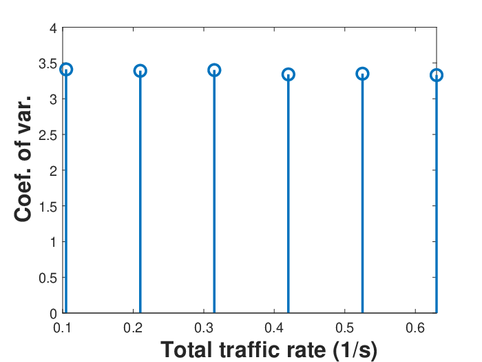
Fig. 3 illustrates the results. The values on the x-axis correspond to the sum of $\lambda$ over all six types for single users. The first value on the x-axis is $0.01+0.02+0.03+0.011+0.019+0.015=0.0905s^{-1}$ . In the second case, we multiply by $2$ the generation rates of every user, hence $2\times$ higher value of the x-axis. This is repeated $6\times$ (hence $6$ values in the plot of Fig. 3). So, the highest value on the x-axis corresponds to traffic generation rates that are $6\times$ higher for all the users than those corresponding to the basic scenario from Table IV.

The interesting outcome from Fig. 3 is that the variability of gNodeB traffic is oblivious to the traffic generation rates of mMTC users ( $c_{V}$ remains almost unchanged at all with the increase in traffic generation rates).

TABLE IV: Basic scenario with heterogeneous mMTC users

Users	$\lambda_{i}$	$N_{i}$	inter-gen. time dist.	number of users
type 1	0.01	(10,20)	uniform	250
type 2	0.02	(10,15)	deterministic	250
type 3	0.03	(10,25)	exponential	250
type 4	0.011	(10,20)	deterministic	250
type 5	0.019	(10,15)	exponential	250
type 6	0.015	(10,15)	uniform	250

IV-D Impact of number of users on gNodeB traffic variability

Having shown the (lack of) impact of traffic generation rates on the variability of network traffic, we look next at how increasing the number of users affects the coefficient of variation of inter-arrival times at gNodeB. We consider the same basic scenario from Table IV, with one exception. The number of users changes from $50$ to $300$ for each user-types, i.e., the total number of users ranges from $300$ to $1800$ . Fig. 6 shows the coefficient of variation for different number of users. As can be observed from Fig. 6, increasing the number of users increases the coefficient of variation of inter-arrival times almost linearly.

IV-E Impact of mMTC distance on traffic characteristics

Having looked at the impact the generation rate and the number of mMTC users have on network traffic variability, we proceed with investigating the impact of distance of mMTC from the base station. The other data are from Table IV. We consider four scenarios to that end. In Scenario 1, each mMTC user is placed uniformly in the range $(0.1,0.5)$ km. In Scenario 2, the range where mMTC are is $(0.1,1)$ km (again uniform), whereas in Scenario 3 every device is placed uniformly in the range $(0.1,2)$ km. Finally, in Scenario 4, the position of each mMTC user is drawn uniformly from the range $(0.1,3)$ km. Needless to say, but mMTC users’ positions are fixed.

Fig. 6 depicts the values of the average inter-arrival times and their $c_{V}$ for the four scenarios. The impact of the distance is almost invisible on the gNodeB traffic characteristics. The reason is that the propagation delay is very low and fixed for every device (mMTC position is fixed), making very little or no impact at all on the network traffic pattern.

IV-F Validation on a dataset

In the last part of this section, we validate our theoretical result for the inter-arrival time at gNodeB. We use a trace of data from $21$ IoT devices as input parameters [11]. More explanations on this dataset can be found in [12]. For every device, we randomly choose a user type and then the corresponding per-block rate from the other trace (Table I). From the dataset [11], it can be observed that data transmission follows different patterns at different devices. In some of these, data are sent uniformly several times during $1$ s, whereas in others every $5$ s. There are no data available on the number of transmitted packets per time. We assume that 30 packets are transmitted at once. The other parameters are as in the previous scenarios. All the users are within the same cell. We observed that the coefficient of variation of inter-generation times for all the users is in the range $(0.5,0.6)$ . Fig. 6 shows the CDF of inter-arrival times at gNodeB from these users. We model the behavior of every user in the system, to the best possible extent, by the corresponding distribution of inter-generation times (the number of packets is fixed whenever there is a transmission). Then, we use Eq.(37) to derive the CDF of the inter-arrival time at gNodeB. Fig. 6 shows this curve as well. As can be observed from Fig. 6, our model can predict quite accurately the inter-arrival time distribution in this realistic scenario, despite the fact that the model may not perfectly capture all the intricacies of the generation process on the users’ side.

V Related Work

While the traffic a single user generates, be it an enhanced Mobile Broadband (eMBB), URLLC, or mMTC, can be determined relatively easily depending on the application/service, predicting the traffic pattern (inter-arrival time and size distribution) at the base station from a (usually) large number of mMTC devices is not straightforward. To our best knowledge, there are no other works that can predict analytically the exact distribution of the traffic pattern at the base station. Regarding the traffic distribution at single mMTC users, the general assumption is that inter-generation times for sparse traffic are either periodic (i.e., deterministic) [13], uniform [14], [15], or exponential [6] for sparse traffic, and for mMTC users with more intense traffic, the number of packets underlie a beta distribution [1], whereas the inter-generation time is governed by a Pareto distribution [14]. In all these models, the sizes of the packets are fixed, and very small. However, in those works, there are no indications as to what distribution the traffic arriving from a large number of mMTC devices to the base station might have. On the other hand, in our paper, we assume a general distribution for the inter-generation times as well as for the number of packets generated at a single mMTC unit, and derive the distribution of the traffic pattern at gNodeB. Furthermore, for most of these single-mMTC traffic distributions, we derive the traffic distribution at gNodeB. We consider as special cases the inter-generation times being deterministic, uniform, exponential, and Pareto distributed. While one of these works [1] assumes the number of generated packets underlies a beta distribution, our approach is more general, as the number of packets underlies any generic distribution, and it can be easily adjusted to capture this special case.

Predicting certain parameters of the traffic arriving at the base station using machine learning is done in [16] and [17]. In [16], the authors propose a supervised learning approach that predicts the number of arrivals and when a burst of data will arrive for the number of packets that follow a beta distribution. However, the service type of interest in [16] is URLLC. On the other hand, in our paper, we derive the exact distribution of both the number of packets arriving at the base station and the inter-arrival time between two data batches for general traffic generations at mMTC users. The main contribution of [17] is proposing a machine learning-based model for predicting possible occurrences of congestion under bursty traffic conditions, where the latter is modeled with a beta distribution. Contrary to [17], our work is more general because deriving the exact distribution of the traffic pattern at gNodeB can also predict whether network congestion is expected to occur for any type of mMTC data distributions.

VI Conclusion

In this paper, we have derived the inter-arrival time distribution of the traffic from different mMTC users within the cell to the base station. We assumed a generic traffic pattern at each mMTC user, specified by a general inter-generation time distribution and a general number of packets transmitted at once. Conducting simulations on a real-life trace, results show that the variability of the traffic pattern increases when increasing the number of mMTC users, but it is not affected by the increase in traffic generation rates. In our future work, we plan to characterize the traffic pattern of the other two service types in 5G - URLLC and eMBB.

References

[1] Y. Wang, T. Wang, Z. Yang, D. Wang, and J. Cheng, “Throughput-oriented non-orthogonal random access scheme for massive MTC networks,” IEEE Transactions on Communications, vol. 68, no. 3, 2020.
[2] G. Ku and J. M. Walsh, “Resource allocation and link adaptation in LTE and LTE Advanced: A tutorial,” IEEE Communications Surveys & Tutorials, vol. 17, no. 3, 2015.
[3] S. E. Elayoubi, S. B. Jemaa, Z. Altman, and A. Galindo-Serrano, “5G RAN slicing for verticals: Enablers and challenges,” IEEE Communications Magazine, vol. 57, no. 1, 2019.
[4] F. Mehmeti and C. Rosenberg, “How expensive is consistency? Performance analysis of consistent rate provisioning to mobile users in cellular networks,” IEEE Tran. on Mob. Computing, vol. 18, no. 5, 2019.
[5] ETSI, “5G NR overall description: 3GPP TS 38.300 version 15.3.1 release 15.” www.etsi.org, 2018. Technical specification.
[6] J. Navarro-Ortiz, P. Romero-Diaz, S. Sendra, P. Ameigeiras, J. J. Ramos-Munoz, and J. M. Lopez-Soler, “A survey on 5G usage scenarios and traffic models,” IEEE Communications Surveys & Tutorials, vol. 22, no. 2, 2020.
[7] S. M. Ross, Stochastic Processes. John Wiley & Sons, 1996.
[8] A. Oppenheim and A. Willsky, Signals and systems. Prentice Hall, 1996.
[9] https://github.com/uccmisl/5Gdataset.
[10] D. Raca, D. Leahy, C. J. Sreenan, and J. J. Quinlan, “Beyond throughput, the next generation: A 5G dataset with channel and context metrics,” in Proc. of ACM MMSys, 2020.
[11] https://research.unsw.edu.au/projects/toniot-datasets.
[12] A. Alsaedi, N. Moustafa, Z. Tari, A. Mahmood, and A. Anwar, “TON IoT telemetry dataset: A new generation dataset of IoT and IIoT for data-driven intrusion detection systems,” IEEE Access, vol. 8, 2020.
[13] Y. Han, S. E. Elayoubi, A. Galindo-Serrano, V. S. Varma, and M. Messai, “Periodic radio resource allocation to meet latency and reliability requirements in 5G networks,” in Proc. of IEEE VTC, 2018.
[14] Q. Hao, Y. Shi, and Q. Zhen, “Study of a traffic model based on adaptive chaotic mapping for mMTC services,” in 11th International Conference on Wireless Communications and Signal Processing (WCSP), 2019.
[15] N. Alhussien and T. A. Gulliver, “Optimal resource allocation in cellular networks with H2H/M2M coexistence,” IEEE Transactions on Vehicular Technology, vol. 69, no. 11, 2020.
[16] T. N. Weerasinghe, I. A. M. Balapuwaduge, and F. Y. Li, “Supervised learning based arrival prediction and dynamic preamble allocation for bursty traffic,” in Proc. of INFOCOM WKSHPS, 2019.
[17] A. Soraa, T. N. Weerasinghe, I. A. M. Balapuwaduge, and F. Y. Li, “Preamble transmission prediction for mMTC bursty traffic: A machine learning based approach,” in Proc. of IEEE GLOBECOM, 2020.