跳到论文正文
W Papers独立论文阅读器 arXiv:2108.00227 论文正文 计算阅读时间 · 0%
引用这篇论文根据当前论文元数据生成,正式投稿前建议核对。


License: CC BY 4.0
arXiv:2108.00227v1 [math.DS] 31 Jul 2021

On the Dynamical System
of Principal Curves in ℝd\mathbb{R}^{d}

Robert Beinert Note: Institute of Mathematics, Technische Universität Berlin, Straße des 17.˜Juni˜136, 10623 Berlin, Germany, {beinert,berdellima,graef,steidl}@math.tu-berlin.de    Arian Bërdëllima11footnotemark: 1    Manuel Gräf11footnotemark: 1    Gabriele Steidl11footnotemark: 1
August 11, 2026
Abstract

Principal curves are natural generalizations of principal lines arising as first principal components in the Principal Component Analysis. They can be characterized—from a stochastic point of view—as so-called self-consistent curves based on the conditional expectation and—from the variational-calculus point of view—as saddle points of the expected difference of a random variable and its projection onto some curve, where the current curve acts as argument of the energy functional. Beyond that, Duchamp and Stützle (1993,1996) showed that planar curves can by computed as solutions of a system of ordinary differential equations. The aim of this paper is to generalize this characterization of principal curves to ℝd\mathbb{R}^{d} with d≥3d\geq 3. Having derived such a dynamical system, we provide several examples for principal curves related to uniform distribution on certain domains in ℝ3\mathbb{R}^{3}.

1 Introduction

Principal component analysis (PCA) [23] is still the working horse of dimensionality reduction algorithms. The dimensionality reduction of data contained in ℝd\mathbb{R}^{d} is here realized by projecting them onto the low-dimensional affine subspace that minimizes the sum of the squared Euclidean distances between the data points and their orthogonal projections. If the affine subspace is one-dimensional, PCA just finds a principal line. Considering the data as realization of a random variable 𝑿:Ω→ℝd\bm{X}:\Omega\to\mathbb{R}^{d}, we may compute the principal line as minimizer of

𝔼⁡[‖𝑿−πg​(𝑿)‖2]\mathbb{E}\left[\|\bm{X}-\pi_{g}(\bm{X})\|^{2}\right] (1)

over all lines gg in ℝd\mathbb{R}^{d}, where πg\pi_{g} denotes the orthogonal projection onto gg. Throughout this paper ∥⋅∥\|\cdot\| denotes the Euclidean norm. There are many attempts to generalize principal lines in the literature. One direction is to replace the linear space ℝd\mathbb{R}^{d} by a nonlinear space. For instance, if ℝd\mathbb{R}^{d} is substituted by a Riemannian manifold, we may ask for the geodesic that minimizes

𝔼⁡[d​(𝑿,πg​(𝑿))2]\mathbb{E}\left[\mathrm{d}(\bm{X},\pi_{g}(\bm{X}))^{2}\right] (2)

over all geodesics gg, where d⁡(⋅,⋅)\mathrm{d}(\cdot,\cdot) denotes the distance on the Riemannian manifold. Among the large amount of literature about PCA on manifolds, we refer to [28, 15, 24, 27] and the references therein.

Another generalization keeps the linear space setting but asks for a smooth curve Γ:[0,ℓ]→ℝd\Gamma:[0,\ell]\rightarrow\mathbb{R}^{d} that is a critical point of

𝔼⁡[‖𝑿−πΓ​(𝑿)‖2].\mathbb{E}\left[\|\bm{X}-\pi_{\Gamma}(\bm{X})\|^{2}\right]. (3)

These curves—called principal curves by Hastie [11] and Hastie & Stützle [12]—possess the so-called self-consistency property, which can be explained via conditional expectations. For principal curves in the plane, Duchamp & Stützle [9] prove that these are indeed saddle points of (3). This is quite contrary to the behaviour of principal lines, which are local minima. Moreover, in the companion paper [8], Duchamp & Stützle show that planar principal curves are solutions of a system of ordinary differential equation. By solving this dynamical system, Duchamp & Stützle find principal curves for uniform densities on rectangles and annuli.

From a numerical point of view, there are several papers on efficient computations of principal-like curves for point clouds, which can seen as finitely many samples with respect to the random variable 𝑿\bm{X}. Usually, these proposed algorithms require additional constraints on the curve [4, 16, 19]. On the basis of these algorithms, principal curves have found applications in image processing like the ice floe identification in satellite images in [1] or like the feature extraction and classification in [3], speech recognition [26], and engineering problems [7]. A more recent generalization of principal curves to manifolds was considered in [13], and principal curves on spheres were discussed in [17].

The aim of this paper is to generalize the characterization of principal curves by differential equations to ℝd\mathbb{R}^{d}, d≥3d\geq 3. Based on our findings, we will compute principal curves for uniform distributions on specific domains. When finishing this paper, we realized that an ingredient of our computation—namely the generalization of the so-called transverse moments to ℝd\mathbb{R}^{d}—has been mentioned in [6], however, without relating the generalized moments to differential equations. Finally, we like to mention an other, completely different, powerful method to approximate arbitrary measures by measures supported on curves based on the minimization of the Wasserstein distance [5, 20] or the discrepancy [10] between such measures.

This paper is organized as follows. In Section 2, we provide necessary preliminaries on probability theory. Then, in Section 3, we recall the definition of principle curves from the stochastic as well as from the variational point of view. The characterization of principal curves by a system of differential equations is derived in Section 4. We apply our findings for computing principal curves with respect to uniform distribution on several domains in ℝ3\mathbb{R}^{3} in Section 5. Finally, we draw conclusions in Section 6.

2 Preliminaries in Probability Theory

In the following, we introduce the necessary notation from probability theory [18]. Let (Ω,𝒜,P)(\Omega,\mathcal{A},P) be a probability space. By ℬ⁡(ℝd)\mathcal{B}(\mathbb{R}^{d}) we denote the Borel-σ\sigma-algebra on ℝd\mathbb{R}^{d}. For a random variable 𝑿=(X1,…,Xd):Ω→ℝd\bm{X}=(X_{1},\ldots,X_{d}):\Omega\to\mathbb{R}^{d}, the push-forward measure P𝑿:ℝd→[0,1]P_{\bm{X}}:\mathbb{R}^{d}\to[0,1] of PP by 𝑿\bm{X} given by

P𝑿​(A):=P⁡(𝑿−1​(A)),A∈ℬ⁡(ℝd),P_{\bm{X}}(A):=P(\bm{X}^{-1}(A)),\qquad A\in\mathcal{B}(\mathbb{R}^{d}),

is called the distribution of 𝑿\bm{X}. We write 𝑿∼P𝑿\bm{X}\sim P_{\bm{X}}. A random variable 𝑿:Ω→ℝd\bm{X}:\Omega\to\mathbb{R}^{d} on a probability space (Ω,𝒜,P)(\Omega,\mathcal{A},P), is called integrable if 𝑿∈L1​(Ω,P)\bm{X}\in L_{1}(\Omega,P), i.e. ∫Ω|𝑿⁡(ω)|​𝑑P​(ω)<∞\int_{\Omega}|\bm{X}(\omega)|\mathrm{d}P(\omega)<\infty. If 𝑿\bm{X} is integrable, then the expectation of 𝑿\bm{X} is defined by

𝔼⁡[𝑿]:=(𝔼⁡[X1],…,𝔼⁡[Xd]),𝔼⁡[Xi]:=∫ΩXi​(ω)​𝑑P​(ω).\mathbb{E}[\bm{X}]:=(\mathbb{E}[X_{1}],\dots,\mathbb{E}[X_{d}]),\quad\mathbb{E}[X_{i}]:=\int_{\Omega}X_{i}(\omega)\mathrm{d}P(\omega).

If 𝑿\bm{X} is square-integrable, i.e. 𝑿∈L2​(Ω,P)\bm{X}\in L_{2}(\Omega,P), then the covariance matrix is defined as

Cov⁡[𝑿]:=(Cov⁡[Xi,Xj])i,j=1d=(𝔼⁡[(Xi−𝔼⁡[Xi])​(Xj−𝔼⁡[Xj])])i,j=1d∈ℝd×d.\mathrm{Cov}[\bm{X}]:=\big(\mathrm{Cov}[X_{i},X_{j}]\big)_{i,j=1}^{d}=\big(\mathbb{E}[(X_{i}-\mathbb{E}[X_{i}])(X_{j}-\mathbb{E}[X_{j}])]\big)_{i,j=1}^{d}\in\mathbb{R}^{d\times d}.

The following theorem, which is a straight-forward generalization of [18, Thm 8.12] from ℝ\mathbb{R} to ℝd\mathbb{R}^{d}, verifies the definition of the conditional expectation of a random variable.

Theorem 2.1.

Let (Ω,𝒜,P)(\Omega,\mathcal{A},P) be a probability space, and let 𝐗:Ω→ℝd\bm{X}:\Omega\to\mathbb{R}^{d} be a random vector with 𝐗∈L1​(Ω,P)\bm{X}\in L_{1}(\Omega,P). For any sub-σ\sigma-algebra ℱ⊂𝒜\mathcal{F}\subset\mathcal{A}, there exists a random variable 𝐙:Ω→ℝd\bm{Z}:\Omega\to\mathbb{R}^{d} with the following properties:

  1. 1.

    𝒁\bm{Z} is ℱ\mathcal{F}-measurable, i.e., 𝒁−1​(B)∈ℱ\bm{Z}^{-1}(B)\in\mathcal{F} for any B∈ℬ⁡(ℝd)B\in\mathcal{B}(\mathbb{R}^{d}), and

  2. 2.

    the expectations are equal on ℱ\mathcal{F}, i.e., for all F∈ℱF\in\mathcal{F} holds

    ∫F𝑿⁡(ω)​𝑑P​(ω)=∫F𝒁⁡(ω)​𝑑P​(ω).\int_{F}\bm{X}(\omega)\mathrm{d}P(\omega)=\int_{F}\bm{Z}(\omega)\mathrm{d}P(\omega).

If 𝐙~:Ω→ℝd\tilde{\bm{Z}}:\Omega\to\mathbb{R}^{d} is another random vector satisfying (i) and (ii), then

P⁡(F∗)=0,F∗:={ω:𝒁⁡(ω)≠𝒁~​(ω)}∈ℱ.P(F_{*})=0,\quad F_{*}:=\{\omega\;:\;\bm{Z}(\omega)\neq\tilde{\bm{Z}}(\omega)\}\in\mathcal{F}.

In particular, 𝐙\bm{Z} is uniquely determined almost everywhere (with respect to the measure P|ℱP|_{\mathcal{F}}).

The random vector 𝒁\bm{Z} is called the conditional expectation of 𝐗\bm{X} given ℱ\mathcal{F}, and we use the notation 𝔼⁡[𝑿|ℱ]:=𝒁\mathbb{E}[\bm{X}|\mathcal{F}]:=\bm{Z}. For 𝑿:Ω→ℝd\bm{X}:\Omega\to\mathbb{R}^{d}, and for a random variable 𝒀:Ω→ℝp\bm{Y}:\Omega\to\mathbb{R}^{p}, we define the conditional expectation of 𝐗\bm{X} given 𝐘\bm{Y} by 𝔼⁡[𝑿|𝒀]:=𝔼⁡[𝑿|σ⁡(𝒀)]:Ω→ℝp\mathbb{E}[\bm{X}|\bm{Y}]:=\mathbb{E}[\bm{X}|\sigma(\bm{Y})]:\Omega\to\mathbb{R}^{p}, where σ⁡(𝒀)\sigma(\bm{Y}) denotes the smallest σ\sigma-algebra containing the set system OPEN{𝒀−1​(B):B∈ℬ⁡(ℝp)})\{\bm{Y}^{-1}(B)\;:\;B\in\mathcal{B}(\mathbb{R}^{p})\}). By the factorization lemma [18, Cor 1.97], there exists a measurable function φ:ℝp→ℝd\varphi:\mathbb{R}^{p}\to\mathbb{R}^{d} such that

𝔼⁡[𝑿|𝒀]​(ω)=φ⁡(𝒀⁡(ω)),ω∈Ω.\mathbb{E}[\bm{X}|\bm{Y}](\omega)=\varphi(\bm{Y}(\omega)),\qquad\omega\in\Omega. (4)

We call φ\varphi the conditional expectation of 𝐗\bm{X} given 𝐘⁡(ω)=𝐲\bm{Y}(\omega)=\bm{y} and use the notation 𝔼⁡[𝑿|𝒀=𝒚]:=φ⁡(𝒚)\mathbb{E}[\bm{X}|\bm{Y}=\bm{y}]:=\varphi(\bm{y}). Denoting by 𝔼𝒀\mathbb{E}_{\bm{Y}} the expectation with respect to probability space (ℝp,ℬ⁡(ℝp),P𝒀)(\mathbb{R}^{p},\mathcal{B}(\mathbb{R}^{p}),P_{\bm{Y}}), where P𝒀P_{\bm{Y}} is the push-forward measure of 𝒀\bm{Y}, we observe

𝔼[𝑿]=∫ℝp𝔼[𝑿|𝒀=𝒚]dP𝒀(𝒚)=𝔼𝒀[𝔼[𝑿|𝒀=⋅]].\mathbb{E}[\bm{X}]=\int_{\mathbb{R}^{p}}\mathbb{E}[\bm{X}|\bm{Y}=\bm{y}]\,\mathrm{d}P_{\bm{Y}}(\bm{y})=\mathbb{E}_{\bm{Y}}\left[\mathbb{E}[\bm{X}|\bm{Y}=\cdot]\right].

3 Principal Curves

Throughout this paper, we consider smooth Jordan curves Γ:[0,ℓΓ]→ℝd\Gamma:[0,\ell_{\Gamma}]\to\mathbb{R}^{d} parameterized by their arc-length. This means that Γ∈C∞​([0,ℓΓ])\Gamma\in C^{\infty}([0,\ell_{\Gamma}]) does not intersect itself, i.e., s1≠s2s_{1}\neq s_{2} implies Γ⁡(s1)≠Γ⁡(s2)\Gamma(s_{1})\neq\Gamma(s_{2}). The distance to the curve is given by d⁡(𝒙,Γ):=min𝒚∈Γ⁡‖𝒙−𝒚‖d(\bm{x},\Gamma):=\min_{\bm{y}\in\Gamma}\|\bm{x}-\bm{y}\|, where the minimum is realized at least once since Γ\Gamma is compact. If 𝒙\bm{x} has several such closest points on Γ\Gamma, then 𝒙\bm{x} is said to be an ambiguity point. The set of ambiguity points 𝒜Γ\mathcal{A}_{\Gamma} is of Lebesgue measure zero, see [11, Lem 4.3.2] and [12, Prop 6]. The projection index λΓ:ℝd→[0,ℓΓ]\lambda_{\Gamma}:\mathbb{R}^{d}\to[0,\ell_{\Gamma}] was introduced by Hastie [11] as

λΓ​(𝒙):=sup{s∈[0,ℓΓ]:‖𝒙−Γ⁡(s)‖=inft∈[0,ℓΓ]‖𝒙−Γ⁡(t)‖},𝒙∈ℝd.\lambda_{\Gamma}(\bm{x}):=\sup\left\{s\in[0,\ell_{\Gamma}]\;:\;\|\bm{x}-\Gamma(s)\|=\inf_{t\in[0,\ell_{\Gamma}]}\|\bm{x}-\Gamma(t)\|\right\},\qquad\bm{x}\in\mathbb{R}^{d}.

Based on the projection index, we define the projection πΓ:ℝd→Γ\pi_{\Gamma}:\mathbb{R}^{d}\to\Gamma as composition 𝒙↦Γ∘λΓ​(𝒙)\bm{x}\mapsto\Gamma\circ\lambda_{\Gamma}(\bm{x}). By slight abuse of notation we identify Γ\Gamma with its image here. Note that the projection is always singe-valued even for the ambiguity points. Hastie [11, Thm 4.1] has shown that λΓ\lambda_{\Gamma} is measurable for smooth curves. Hence, for a random variable 𝑿:Ω→ℝd\bm{X}:\Omega\rightarrow\mathbb{R}^{d}, the composition λΓ∘𝑿:Ω→[0,ℓΓ]\lambda_{\Gamma}\circ\bm{X}:\Omega\to[0,\ell_{\Gamma}] is also a random variable as well as Γ​(λΓ​(𝑿))\Gamma(\lambda_{\Gamma}(\bm{X})), and we have πΓ​(𝑿)=Γ⁡(λΓ​(𝑿))\pi_{\Gamma}(\bm{X})=\Gamma(\lambda_{\Gamma}(\bm{X})). By the factorization in (4), we can write the conditional expectation as

𝔼⁡[𝑿|λΓ∘𝑿]​(ω)=ϕ∘λΓ∘𝑿⁡(ω),\mathbb{E}[\bm{X}|\lambda_{\Gamma}\circ\bm{X}](\omega)=\phi\circ\lambda_{\Gamma}\circ\bm{X}(\omega), (5)

with 𝔼⁡[𝑿|λΓ​(𝑿)=s]=ϕ⁡(s)\mathbb{E}[\bm{X}|\lambda_{\Gamma}(\bm{X})=s]=\phi(s). A curve Γ\Gamma is called self-consistent if and only if

𝔼⁡[𝑿|λΓ​(𝑿)=s]=Γ⁡(s)PλΓ​(𝑿)−a.e.\mathbb{E}[\bm{X}|\lambda_{\Gamma}(\bm{X})=s]=\Gamma(s)\qquad P_{\lambda_{\Gamma}(\bm{X})}-\text{a.e.}

for all s∈[0,ℓΓ]s\in[0,\ell_{\Gamma}]. A smooth, self-consistent Jordan curve is called a principal curve of 𝑿\bm{X} [12].

For uniformly distributed random variables 𝑿:Ω→ℝ2\bm{X}:\Omega\rightarrow\mathbb{R}^{2}, the definition says that a principal curve is characterized by the fact that the barycenter of the region λΓ−1​(I)\lambda^{-1}_{\Gamma}(I) related to some interval I⊂[0,ℓΓ]I\subset[0,\ell_{\Gamma}] converges to Γ\Gamma if the length of II becomes arbitrary small. Numerically, some example regions λΓ−1​(I)\lambda^{-1}_{\Gamma}(I) may be calculated using the Voronoi cells with respect to finitely many samples on Γ\Gamma, which allow a numerical validation whether a curve is principal for a given uniform distribution. This definition and numerical interpretation is illustrated in Figure 1.

Refer to caption
Refer to caption
Figure 1: Two examples for curves and uniformly distributed random variable 𝑿\bm{X}. Left: 𝑿\bm{X} corresponds to the uniform distribution on the quarter circle of radius 1. Its principal curve is just the quarter circle of radius 23\frac{2}{3}. The barycenters of the Voronoi cells converge to the curve if the curve is sampled denser. Right: 𝑿\bm{X} corresponds to the uniform distribution on the square of side length 1. For a quarter parabolic curve (blue dots), we calculate the barycenters (red dots) of the corresponding Voronoi cells. These centers do not converge to the curve even if the regions become arbitrary thin; so the shown curve is not principal.

Principal curves have a nice variational characterization. To this end, we consider the energy functional

D𝑿2​(Γ):=𝔼⁡[‖𝑿−Γ⁡(λΓ​(𝑿))‖2],D_{\bm{X}}^{2}(\Gamma):=\mathbb{E}[\|\bm{X}-\Gamma(\lambda_{\Gamma}(\bm{X}))\|^{2}], (6)

whose critical points are principal curves.

Theorem 3.1 (Hastie & Stuetzle [12, Prop 4]).

Let 𝐗:Ω→ℝd\bm{X}:\Omega\rightarrow\mathbb{R}^{d} be a random variable with finite covariance and smooth density. Further, let Γ:[0,ℓΓ]→ℝd\Gamma:[0,\ell_{\Gamma}]\to\mathbb{R}^{d} be a smoooth Jordan curve parameterized by arc-length. Then the curve Γ\Gamma is a principal curve of 𝐗\bm{X} if and only if

d​D𝑿2​(Γ+t​Δ)d​t|t=0=0,\frac{\mathrm{d}D_{\bm{X}}^{2}(\Gamma+t\Delta)}{\mathrm{d}t}\Big|_{t=0}=0,

for any curve Δ∈C∞​([0,ℓΓ])\Delta\in C^{\infty}([0,\ell_{\Gamma}]) with ‖Δ‖≤1\|\Delta\|\leq 1, ‖Δ′‖≤1\|\Delta^{\prime}\|\leq 1.

4 Characterization via Differential Equations

A third characterization of principal curves in the plane is given by a dynamical system [8]. In this section, we generalize the derivation to curves Γ:[0,ℓΓ]→ℝd\Gamma:[0,\ell_{\Gamma}]\rightarrow\mathbb{R}^{d} in higher dimensions, i.e. d≥2d\geq 2. For this, we associate to Γ⁡(s)\Gamma(s) a reference frame T⁡(s),N1​(s),…,Nd−1​(s)∈𝕊d−1T(s),N_{1}(s),\dots,N_{d-1}(s)\in\mathbb{S}^{d-1} smoothly depending on ss, where T⁡(s):=Γ′​(s)∈𝕊d−1T(s):=\Gamma^{\prime}(s)\in\mathbb{S}^{d-1} denotes the tangent, and where N1​(s),…,Nd−1​(s)N_{1}(s),\dots,N_{d-1}(s) are pairwise orthogonal vectors spanning the normal space of Γ\Gamma in s∈[0,ℓΓ]s\in[0,\ell_{\Gamma}]. Recall that the curvature of a curve is given by κ⁡(s):=‖T′​(s)‖\kappa(s):=\|T^{\prime}(s)\|. The principal curvatures with respect to the chosen moving reference frame are now defined by

κi(s):=⟨T′(s),Ni(s)⟩,i=1,…,d−1.\kappa_{i}(s):=\langle T\,^{\prime}(s),N_{i}(s)\rangle,\qquad i=1,\dots,d-1. (7)

In other words, the principal curvatures (κ1,…,κd−1)(\kappa_{1},\dots,\kappa_{d-1}) are the coordinates of the normal Γ′′=T′\Gamma^{\prime\prime}=T^{\prime} with respect to the frame N1,…,Nd−1N_{1},\dots,N_{d-1}. Due to the orthogonality ⟨T,Ni⟩=0\langle T,N_{i}\rangle=0, we have

0=dd​s⟨T(s),Ni(s)⟩=⟨T′(s),Ni(s)⟩+⟨T(s),Ni′(s)⟩,i=1,…,d−1,0=\frac{d}{ds}\langle T(s),N_{i}(s)\rangle=\langle T^{\prime}(s),N_{i}(s)\rangle+\langle T(s),N_{i}^{\prime}(s)\rangle,\qquad i=1,\dots,d-1,

implying

κi(s)=−⟨T,Ni′(s)⟩,i=1,…,d−1.\kappa_{i}(s)=-\langle T,N_{i}^{\prime}(s)\rangle,\qquad i=1,\dots,d-1. (8)

There are different kind of frames in the literature, e.g., the Frenet frame, the Bishop frame, and various modifications [2, 29]. The Frenet frame is unique, but may fail to be well defined at certain points even if the curve is sufficiently regular. In contrast, the Bishop frame—also known as parallel frame—is defined at every point and varies continuously as we move along the curve. This frame is described by the system of first order differential equations

[T′​(s)N1′​(s)N2′​(s)Nd−1′​(s)]=[0κ1​(s)κ2​(s)⋯κd−1​(s)−κ1​(s)00⋯0−κ2​(s)00⋯0⋱−κd−1​(s)00⋯0]⋅[T⁡(s)N1​(s)N2​(s)Nd−1​(s)].\displaystyle\begin{bmatrix}T^{\prime}(s)\\ N_{1}^{\prime}(s)\\ N_{2}^{\prime}(s)\\ \vdots\\ N_{d-1}^{\prime}(s)\end{bmatrix}=\begin{bmatrix}0&\kappa_{1}(s)&\kappa_{2}(s)&\cdots&\kappa_{d-1}(s)\\ -\kappa_{1}(s)&0&0&\cdots&0\\ -\kappa_{2}(s)&0&0&\cdots&0\\ \vdots&\vdots&\vdots&\ddots&\vdots\\ -\kappa_{d-1}(s)&0&0&\cdots&0\end{bmatrix}\cdot\begin{bmatrix}T(s)\\ N_{1}(s)\\ N_{2}(s)\\ \vdots\\ N_{d-1}(s)\end{bmatrix}. (9)

In the numerical part, we will rely on a different frame based on spherical coordinates.

Henceforth, let 𝕏\mathbb{X} be a compact region in ℝd\mathbb{R}^{d}, which will later denote the support of the density p𝑿p_{\bm{X}}. The normal coordinate map of Γ\Gamma with respect to the chosen reference frame is the map νΓ:[0,ℓΓ]×ℝd−1→ℝd\nu_{\Gamma}:[0,\ell_{\Gamma}]\times\mathbb{R}^{d-1}\to\mathbb{R}^{d} given by

νΓ(s,u1,…,ud−1)≔Γ(s)+u1N1(s)+⋯ud−1Nd−1(s),\nu_{\Gamma}(s,u_{1},\dots,u_{d-1})\coloneqq\Gamma(s)+u_{1}\,N_{1}(s)+\cdots u_{d-1}\,N_{d-1}(s), (10)

and the normal coordinate transformation μΓ:𝕏→[0,ℓΓ]×ℝd−1\mu_{\Gamma}:\mathbb{X}\to[0,\ell_{\Gamma}]\times\mathbb{R}^{d-1} is defined by

μΓ​(𝒙)≔(λΓ​(𝒙)⟨𝒙−πΓ​(𝒙),N1​(λ⁡(𝒙))⟩⟨𝒙−πΓ​(𝒙),Nd−1​(λ⁡(𝒙))⟩).\mu_{\Gamma}(\bm{x})\coloneqq\begin{pmatrix}\lambda_{\Gamma}(\bm{x})\\ \langle\bm{x}-\pi_{\Gamma}(\bm{x}),N_{1}(\lambda(\bm{x}))\rangle\\ \vdots\\ \langle\bm{x}-\pi_{\Gamma}(\bm{x}),N_{d-1}(\lambda(\bm{x}))\rangle\end{pmatrix}. (11)

The components (s,u1,…,ud−1)(s,u_{1},\dots,u_{d-1}) of μΓ​(𝒙)\mu_{\Gamma}(\bm{x}) are called the normal coordinates at 𝒙\bm{x}. For given s∈[0,ℓΓ]s\in[0,\ell_{\Gamma}], let 𝕏⁡(s)\mathbb{X}(s) be the cross-section of 𝕏\mathbb{X} with the hyperplane Γ⁡(s)+u1​N1​(s)+⋯+ud−1​Nd−1​(s)\Gamma(s)+u_{1}N_{1}(s)+\cdots+u_{d-1}N_{d-1}(s). The normal coordinates around Γ⁡(s)\Gamma(s) in 𝕏⁡(s)\mathbb{X}(s) are denoted by

ℛ(s)={(u1,…,ud−1)∈ℝd−1:\displaystyle\mathcal{R}(s)=\{(u_{1},\dots,u_{d-1})\in\mathbb{R}^{d-1}\;:\; πΓ​(Γ⁡(s)+u1​N1​(s)+⋯+ud−1​Nd−1​(s))=s,\displaystyle\pi_{\Gamma}(\Gamma(s)+u_{1}N_{1}(s)+\cdots+u_{d-1}N_{d-1}(s))=s,
Γ(s)+u1N1(s)+⋯+ud−1Nd−1(s)∉𝒜Γ}.\displaystyle\Gamma(s)+u_{1}N_{1}(s)+\cdots+u_{d-1}N_{d-1}(s)\not\in\mathcal{A}_{\Gamma}\}.

For the later substitution, we need that νΓ\nu_{\Gamma} is a diffeomorphism on (λΓ−1​(I)∩𝕏)∖𝒜Γ(\lambda_{\Gamma}^{-1}(I)\cap\mathbb{X})\setminus\mathcal{A}_{\Gamma} for all measurable I⊆[0,ℓΓ]I\subseteq[0,\ell_{\Gamma}] meaning that

(νΓ∘μΓ)|(λΓ−1​(I)∩𝕏)∖𝒜Γ=id|(λΓ−1​(I)∩𝕏)∖𝒜Γ,(\nu_{\Gamma}\circ\mu_{\Gamma})|_{(\lambda_{\Gamma}^{-1}(I)\cap\mathbb{X})\setminus\mathcal{A}_{\Gamma}}=\id|_{(\lambda_{\Gamma}^{-1}(I)\cap\mathbb{X})\setminus\mathcal{A}_{\Gamma}},

and that νΓ\nu_{\Gamma} and μΓ\mu_{\Gamma} are differentiable on the related domains. The partial derivatives of νΓ\nu_{\Gamma} are given by

∂νΓ∂s\displaystyle\frac{\partial\nu_{\Gamma}}{\partial s} =Γ′(s)+u1N′1(s)+⋯ud−1N′d−1(s),\displaystyle=\Gamma^{\prime}(s)+u_{1}\,N^{\prime}_{1}(s)+\cdots u_{d-1}\,N^{\prime}_{d-1}(s),
∂νΓ∂ui\displaystyle\frac{\partial\nu_{\Gamma}}{\partial u_{i}} =Ni(s),i=1,…,d−1.\displaystyle=N_{i}(s),\qquad i=1,\dots,d-1.

Using (8), and exploiting the orthonormality of the frame, we obtain the Jacobian determinant

|det(𝑱νΓ)|​(s,𝒖)\displaystyle|\det(\bm{J}_{\nu_{\Gamma}})|(s,\bm{u}) =|T(s)+u1N1′(s)+⋯+ud−1Nd−1′(s),N1(s),…,Nd−1(s)|\displaystyle=|T(s)+u_{1}\,N_{1}^{\prime}(s)+\cdots+u_{d-1}\,N_{d-1}^{\prime}(s),N_{1}(s),\dots,N_{d-1}(s)|
=|⟨T(s),T(s)+u1N1′(s)+⋯+ud−1Nd−1′(s)⟩T(s),N1(s),…,Nd−1(s)|\displaystyle=|\langle T(s),T(s)+u_{1}\,N_{1}^{\prime}(s)+\cdots+u_{d-1}\,N_{d-1}^{\prime}(s)\rangle T(s),N_{1}(s),\dots,N_{d-1}(s)|
=1+u1​⟨T⁡(s),N1′​(s)⟩+⋯+ud−1​⟨T⁡(s),Nd−1′​(s)⟩\displaystyle=1+u_{1}\langle T(s),N_{1}^{\prime}(s)\rangle+\cdots+u_{d-1}\langle T(s),N_{d-1}^{\prime}(s)\rangle
=1−u1​κ1−⋯−ud−1​κd−1.\displaystyle=1-u_{1}\kappa_{1}-\cdots-u_{d-1}\kappa_{d-1}.

Now we can describe the self-consistency of curves with respect to a random variable based on its transverse moments

μ𝒋(s):=∫𝒖∈ℛ⁡(s)u1j1⋯ud−1jd−1p𝑿(Γ(s)+∑i=1d−1uiNi(s))d𝒖,𝒋∈ℕ0d−1.\mu_{\bm{j}}(s):=\int\limits_{\bm{u}\in\mathcal{R}(s)}u_{1}^{j_{1}}\cdots u_{d-1}^{j_{d-1}}\,p_{\bm{X}}\Big(\Gamma(s)+\sum_{i=1}^{d-1}u_{i}\,N_{i}(s)\Big)\,d\bm{u},\qquad\bm{j}\in\mathbb{N}_{0}^{d-1}. (12)

Further, the canonical basis of ℝd−1\mathbb{R}^{d-1} is denoted by 𝒆1,…,𝒆d−1∈ℝd−1\bm{e}_{1},\dots,\bm{e}_{d-1}\in\mathbb{R}^{d-1}.

Theorem 4.1.

Let 𝐗:Ω→ℝd\bm{X}:\Omega\rightarrow\mathbb{R}^{d} be a random variable having a distribution with smooth density function p𝐗p_{\bm{X}}, where supp​p𝐗=𝕏\mathrm{supp}\,p_{\bm{X}}=\mathbb{X} and p𝐗p_{\bm{X}} is strictly positive in the interior of 𝕏\mathbb{X}. We consider smooth Jordan curves Γ:[0,ℓΓ]→𝕏\Gamma:[0,\ell_{\Gamma}]\rightarrow\mathbb{X} for which νΓ\nu_{\Gamma} is a diffeomorphism on (λΓ−1​([0,ℓΓ])∩𝕏)∖𝒜Γ(\lambda_{\Gamma}^{-1}([0,\ell_{\Gamma}])\cap\mathbb{X})\setminus\mathcal{A}_{\Gamma}. Then Γ\Gamma is self-consistent with respect 𝐗\bm{X} if and only if its principal curvature κ\mathbf{\kappa} fulfills the linear system of equations

𝝁⁡(s)=𝑮⁡(s)​(κ1​(s),…,κd−1​(s))T\bm{\mu}(s)=\bm{G}(s)\big(\kappa_{1}(s),\dots,\kappa_{d-1}(s)\big)^{\mathrm{T}} (13)

with

𝑮⁡(s):=(μ𝒆i+𝒆j​(s))i,j=1d−1,𝝁⁡(s):=(μ𝒆i​(s))i=1d−1.\bm{G}(s):=\big(\mu_{\bm{e}_{i}+\bm{e}_{j}}(s)\big)_{i,j=1}^{d-1},\quad\bm{\mu}(s):=\big(\mu_{\bm{e}_{i}}(s)\big)_{i=1}^{d-1}.

The Gram matrix 𝐆⁡(s)\bm{G}(s) is invertible, so that

κj=(𝑮−1𝝁)j,j=1,…,d−1.\kappa_{j}=(\bm{G}^{-1}\bm{\mu})_{j},\qquad j=1,\dots,d-1. (14)
Proof.

Based on Theorem 2.1 and the factorization of the conditional expectation in (5), for all measurable sets I⊆[0,ℓΓ]I\subseteq[0,\ell_{\Gamma}], the self-consistency ϕ⁡(s)=𝔼⁡[𝑿|λΓ​(𝑿)=s]=Γ⁡(s)\phi(s)=\mathbb{E}[\bm{X}|\lambda_{\Gamma}(\bm{X})=s]=\Gamma(s) means

∫(λΓ∘𝑿)−1​(I)𝑿⁡(ω)​𝑑P​(ω)\displaystyle\int_{(\lambda_{\Gamma}\circ\bm{X})^{-1}(I)}\bm{X}(\omega)\,dP(\omega) =∫(λΓ∘𝑿)−1​(I)𝔼⁡[𝑿|λΓ∘𝑿]​(ω)​𝑑P​(ω)=∫(λΓ∘𝑿)−1​(I)(ϕ∘λΓ∘𝑿)​(ω)​𝑑P​(ω)\displaystyle=\int_{(\lambda_{\Gamma}\circ\bm{X})^{-1}(I)}\mathbb{E}[\bm{X}|\lambda_{\Gamma}\circ\bm{X}](\omega)\,dP(\omega)=\int_{(\lambda_{\Gamma}\circ\bm{X})^{-1}(I)}(\phi\circ\lambda_{\Gamma}\circ\bm{X})(\omega)\,dP(\omega)
=∫(λΓ∘𝑿)−1​(I)(Γ∘λΓ∘𝑿)​(ω)​𝑑P​(ω).\displaystyle=\int_{(\lambda_{\Gamma}\circ\bm{X})^{-1}(I)}(\Gamma\circ\lambda_{\Gamma}\circ\bm{X})(\omega)\,dP(\omega).

This can be rewritten as

∫λΓ−1​(I)𝒙​p𝑿​(𝒙)​𝑑𝒙=∫λΓ−1​(I)(Γ∘λΓ)​(𝒙)​p𝑿​(𝒙)​𝑑𝒙=∫λΓ−1​(I)πΓ​(𝒙)​p𝑿​(𝒙)​𝑑𝒙\int_{\lambda^{-1}_{\Gamma}(I)}\bm{x}\,p_{\bm{X}}(\bm{x})\,d\bm{x}=\int_{\lambda^{-1}_{\Gamma}(I)}(\Gamma\circ\lambda_{\Gamma})(\bm{x})\,p_{\bm{X}}(\bm{x})\,d\bm{x}=\int_{\lambda^{-1}_{\Gamma}(I)}\pi_{\Gamma}(\bm{x})\,p_{\bm{X}}(\bm{x})\,d\bm{x} (15)

or, equivalently,

∫λΓ−1​(I)(𝒙−πΓ​(𝒙))​p𝑿​(𝒙)​𝑑𝒙=0\int_{\lambda^{-1}_{\Gamma}(I)}(\bm{x}-\pi_{\Gamma}(\bm{x}))\,p_{\bm{X}}(\bm{x})\,d\bm{x}=0 (16)

for all measurable sets I⊆[0,ℓΓ]I\subseteq[0,\ell_{\Gamma}]. Regarding that νΓ\nu_{\Gamma} is a diffeomorphism on (λΓ−1​(I)∩𝕏)∖𝒜Γ(\lambda_{\Gamma}^{-1}(I)\cap\mathbb{X})\setminus\mathcal{A}_{\Gamma}, and that 𝒜Γ\mathcal{A}_{\Gamma} is a null set, we can rewrite the last integral condition in terms of the normal coordinates

∬(s,𝒖)∈μΓ​(λΓ−1​(I)∖𝒜Γ)(∑i=1d−1ui​Ni​(s))​p𝑿​(Γ⁡(s)+∑i=1d−1ui​Ni​(s))​|det(𝑱νΓ)|​𝑑𝒖​𝑑s=0.\iint\limits_{(s,\bm{u})\in\mu_{\Gamma}\left(\lambda^{-1}_{\Gamma}(I)\setminus\mathcal{A}_{\Gamma}\right)}\Big(\sum_{i=1}^{d-1}u_{i}\,N_{i}(s)\Big)\,p_{\bm{X}}\Big(\Gamma(s)+\sum_{i=1}^{d-1}u_{i}\,N_{i}(s)\Big)\,|\det(\bm{J}_{\nu_{\Gamma}})|d\bm{u}\,ds=0.

Since the above equation holds for all I⊆[0,ℓΓ]I\subseteq[0,\ell_{\Gamma}], the integrand with respect to ss thus has to be zero almost surely, i.e.

∫𝒖∈ℛ⁡(s)(∑i=1d−1ui​Ni​(s))​p𝑿​(Γ⁡(s)+∑i=1d−1ui​Ni​(s))​|det(𝑱νΓ)|​𝑑𝒖=0,s​-a.s.\int\limits_{\bm{u}\in\mathcal{R}(s)}\Big(\sum_{i=1}^{d-1}u_{i}\,N_{i}(s)\Big)\,p_{\bm{X}}\Big(\Gamma(s)+\sum_{i=1}^{d-1}u_{i}\,N_{i}(s)\Big)\,|\det(\bm{J}_{\nu_{\Gamma}})|\,d\bm{u}=0,\quad s\text{-a.s.} (17)

Exploiting that the of Ni​(s)N_{i}(s) are orthonormal and the smoothness of p𝑿p_{\bm{X}}, we see that the parameter integral is continuous, so that we obtain

∫𝒖∈ℛ⁡(s)ujp𝑿(Γ(s)+∑i=1d−1uiNi(s))(1−∑i=1d−1uiκi(s))d𝒖=0,j=1,…,d−1\displaystyle\int\limits_{\bm{u}\in\mathcal{R}(s)}u_{j}\,p_{\bm{X}}\Big(\Gamma(s)+\sum_{i=1}^{d-1}u_{i}\,N_{i}(s)\Big)\,\Big(1-\sum_{i=1}^{d-1}u_{i}\kappa_{i}(s)\Big)\,d\bm{u}=0,\qquad j=1,\dots,d-1 (18)

for all s∈[0,ℓΓ]s\in[0,\ell_{\Gamma}]. Note that the Jacobian determinant is here always positive, since μΓ\mu_{\Gamma} and νΓ\nu_{\Gamma} are diffeomorphisms. Using the transverse moments notation in (12) this can be rewritten as the system (13). Since the first-order monomials 𝒖↦ui\bm{u}\mapsto u_{i}, i=1,…,d−1i=1,\dots,d-1, are linear independent on every open subset in ℝd−1\mathbb{R}^{d-1}, we infer that the Gram matrix 𝑮\bm{G} is invertible. ∎

In the following, we fix the moving reference frame by parameterizing the tangent vector using spherical coordinates

T⁡(𝜻):=(cos⁡(ζ1)sin⁡(ζ1)​cos⁡(ζ2)sin⁡(ζ1)​sin⁡(ζ2)​cos⁡(ζ3)sin(ζ1)sin(ζ2)⋯sin(ζd−2)cos(ζd−1)sin(ζ1)sin(ζ2)⋯sin(ζd−2)sin(ζd−1))∈𝕊d−1T(\bm{\zeta}):=\begin{pmatrix}&\cos(\zeta_{1})\\ &\sin(\zeta_{1})\cos(\zeta_{2})\\ &\sin(\zeta_{1})\sin(\zeta_{2})\cos(\zeta_{3})\\ &\vdots\\ &\sin(\zeta_{1})\sin(\zeta_{2})\cdots\sin(\zeta_{d-2})\cos(\zeta_{d-1})\\ &\sin(\zeta_{1})\sin(\zeta_{2})\cdots\sin(\zeta_{d-2})\sin(\zeta_{d-1})\end{pmatrix}\in\mathbb{S}^{d-1} (19)

where ζi∈[0,π]\zeta_{i}\in[0,\pi], i=1,…,d−2i=1,\dots,d-2 and ζd−1∈[0,2​π)\zeta_{d-1}\in[0,2\pi) are functions of ss. Note that T⁡(𝜻)T(\bm{\zeta}) and its partial derivatives Tζi:=dd​ζi​TT_{\zeta_{i}}:=\frac{d}{d\zeta_{i}}T satisfy the recursions

T⁡(𝜻)=(cos⁡(ζ1)sin⁡(ζ1)​T​(𝝃)),Tζ1​(𝜻)=(−sin⁡(ζ1)cos⁡(ζ1)​T​(𝝃)),Tζk​(𝜻)=sin⁡(ζ1)​(0Tξk−1​(𝝃)),T(\bm{\zeta})=\begin{pmatrix}\cos(\zeta_{1})\\ \sin(\zeta_{1})\,T(\bm{\xi})\end{pmatrix},\qquad T_{\zeta_{1}}(\bm{\zeta})=\begin{pmatrix}-\sin(\zeta_{1})\\ \cos(\zeta_{1})\,T(\bm{\xi})\end{pmatrix},\qquad T_{\zeta_{k}}(\bm{\zeta})=\sin(\zeta_{1})\begin{pmatrix}0\\ T_{\xi_{k-1}}(\bm{\xi})\end{pmatrix}, (20)

where 𝝃:=(ζ2,…,ζd−1)T\bm{\xi}:=(\zeta_{2},\dots,\zeta_{d-1})^{\mathrm{T}}. Consequently, we have ‖Tζ1‖=1\|T_{\zeta_{1}}\|=1 and ‖Tζk‖=∏i=1k−1sin⁡(ζi)\|T_{\zeta_{k}}\|=\prod_{i=1}^{k-1}\sin(\zeta_{i}), k=2,…,d−1k=2,\ldots,d-1. Defining the vectors

Ni​(ζ):=Tζi​(ζ)‖Tζi​(ζ)‖i=1,…,d−1,N_{i}(\mathbf{\zeta}):=\frac{T_{\zeta_{i}}(\mathbf{\zeta})}{\|T_{\zeta_{i}}(\mathbf{\zeta})\|}\qquad i=1,\dots,d-1,

for ζk∉{0,π}\zeta_{k}\not\in\{0,\pi\}, k=1,…,d−2k=1,\ldots,d-2, we see that {T⁡(ξ),N1​(ξ),…,Nd−1​(ξ)}\{T(\mathbf{\xi}),N_{1}(\mathbf{\xi}),\ldots,N_{d-1}(\mathbf{\xi})\} forms an orthonormal basis of ℝd\mathbb{R}^{d}. Later we will argue that the instabilities are not problematic for the numerical part.

Considering the curvature of Γ\Gamma given by

dd​s​T​(s)=∑i=1d−1ζi′​(s)​Tζi​(s),\frac{d}{ds}T(s)=\sum_{i=1}^{d-1}\zeta_{i}^{\prime}(s)T_{\zeta_{i}}(s),

we conclude from (7) that

κi(s)=⟨dd​sT(s),Ni(s)⟩=ζi′(s)∥Tζi(s)∥,i=1,…,d−1.\kappa_{i}(s)=\left\langle\frac{d}{ds}T(s),N_{i}(s)\right\rangle=\zeta_{i}^{\prime}(s)\|T_{\zeta_{i}}(s)\|,\qquad i=1,\dots,d-1. (21)

Inserting these identities into (14), the self-consistency of a curve with respect to 𝐗\mathbf{X} is equivalent to the system of differential equations

Γ′​(s)\displaystyle\Gamma^{\prime}(s) =T⁡(ζ⁡(s)),\displaystyle=T(\zeta(s)), (22)
ζj′​(s)\displaystyle\zeta^{\prime}_{j}(s) =(𝑮−1​𝝁)j/‖Tζi​(s)‖=(𝑮−1​𝝁)j/∏k=1i−1sin⁡(ζk).\displaystyle=(\bm{G}^{-1}\bm{\mu})_{j}/\|T_{\zeta_{i}(s)}\|=(\bm{G}^{-1}\bm{\mu})_{j}\Bigm/\penalty\prod_{k=1}^{i-1}\sin(\zeta_{k}).

Note that the moments μ𝒋​(s)\mu_{\bm{j}}(s) are functions depending both on the point Γ⁡(s)\Gamma(s) and our specific frame characterized by 𝜻⁡(s)\bm{\zeta}(s). Therefore the right-hand side of the differential equation system is a function in (Γ⁡(s),𝜻⁡(s))(\Gamma(s),\bm{\zeta}(s)) and may be solved using linear multistep methods for instance.

The first and second order transverse moments can be interpreted stochastically by defining the transverse density at time ss by

p⟂​(𝒖,s)≔p⁡(Γ⁡(s)+u1​N1​(𝜻⁡(s))+⋯+ud−1​Nd−1​(𝜻⁡(s)))μ𝟎​(s),𝒖∈ℛ⁡(s).p_{\perp}(\bm{u},s)\coloneqq\frac{p(\Gamma(s)+u_{1}N_{1}(\bm{\zeta}(s))+\cdots+u_{d-1}N_{d-1}(\bm{\zeta}(s)))}{\mu_{\bm{0}}(s)},\quad\bm{u}\in\mathcal{R}(s). (23)

The mean and the covariance matrix of the transverse density p⟂​(⋅,s)p_{\perp}(\cdot,s) with respect to the normal coordinates are given by

v⟂​(s)\displaystyle v_{\perp}(s) :=(μ𝒆1​(s)μ𝟎​(s),…,μ𝒆d−1​(s)μ𝟎​(s))T,\displaystyle:=\Big(\frac{\mu_{\bm{e}_{1}}(s)}{\mu_{\bm{0}}(s)},\dots,\frac{\mu_{\bm{e}_{d-1}}(s)}{\mu_{\bm{0}}(s)}\Big)^{\mathrm{T}},
cov⟂​(s)\displaystyle\mathrm{cov}_{\perp}(s) :=(μ𝒆i+𝒆j​(s)μ𝟎​(s))i,j=1d−1−v⟂​(s)​v⟂​(s)T.\displaystyle:=\Big(\frac{\mu_{\bm{e}_{i}+\bm{e}_{j}}(s)}{\mu_{\bm{0}}(s)}\Big)_{i,j=1}^{d-1}-v_{\perp}(s)\,v_{\perp}(s)^{\mathrm{T}}.

Since the 0th transverse moment cancels out, we arrive at the ordinary system of differential equations

Γ′​(s)\displaystyle\Gamma^{\prime}(s) =T⁡(ζ⁡(s))\displaystyle=T(\zeta(s)) (24)
𝜻′​(s)\displaystyle\bm{\zeta}^{\prime}(s) =D−1​(s)​(cov⟂​(s)+v⟂​(s)​v⟂​(s)T)−1​v⟂​(s)\displaystyle=D^{-1}(s)\Big(\mathrm{cov}_{\perp}(s)+v_{\perp}(s)v_{\perp}(s)^{\mathrm{T}}\Big)^{-1}v_{\perp}(s)

with

D⁡(s):=diag⁡(‖Tζ1​(s)‖,…,‖Tζd−1​(s)‖).D(s):=\diag(\|T_{\zeta_{1}}(s)\|,\dots,\|T_{\zeta_{d-1}}(s)\|).

Our findings are summarized in the following theorem.

Theorem 4.2.

Let the assumptions of Theorem 4.1 be fulfilled. Assume that Γ\Gamma can be represented by the above frame with ζk​(s)∉{0,π}\zeta_{k}(s)\not\in\{0,\pi\}, k=1,…,d−2k=1,\ldots,d-2, s∈[0,ℓΓ]s\in[0,\ell_{\Gamma}]. Then the curve Γ\Gamma is self-consistent with respect to 𝐗\bm{X} if and only if it is a solution of the system of differential equations (24).

From a numerical point of view the above instabilities causes by the ambiguousness of the spherical coordinates appear to be non-problematic. Notice that the scenery, i.e. the random variable 𝑿\bm{X} with density p𝑿p_{\bm{X}}, the starting point Γ⁡(0)\Gamma(0), and the initial tangent Γ′​(0)\Gamma^{\prime}(0) may be rotated such that the spherical coordinates of Γ′​(0)\Gamma^{\prime}(0) satisfy ζk∉{0,π}\zeta_{k}\not\in\{0,\pi\}, k=1,…,d−2k=1,\ldots,d-2. If the solution of (24) is computed step-by-step by a linear multistep method, we may stop the computation whenever the spherical coordinates of the tangent become ambiguous. Rotating the scenery with the computed curve again, we can continue the computations.

5 Principal Curves of Uniformly Distributed Random Variables

In this section, we are interested in the concrete computation of principal curves of uniformly distributed random variables with densities supported at certain specific domains in ℝ3\mathbb{R}^{3}. For the numerics and the considerations on symmetries, we have to assume that Γ\Gamma fulfills the following admissibility assumptions:

  1. 1.

    𝕏\mathbb{X} contains no ambiguity points with respect to Γ\Gamma. This implies that the normal map is the left inverse of the normal coordinate map

    νΓ∘μΓ=id𝕏,\nu_{\Gamma}\circ\mu_{\Gamma}=\id_{\mathbb{X}}, (25)
  2. 2.

    the map νΓ:[0,ℓΓ]×ℝd−1→ℝd\nu_{\Gamma}:\ [0,\ell_{\Gamma}]\times\mathbb{R}^{d-1}\to\mathbb{R}^{d} is a diffeomorphism onto its image.

Excluding any ambiguity points, we are able to compute the transverse moments μ𝒋​(s)\mu_{\bm{j}}(s) in (12) by only knowing the current position Γ⁡(s)\Gamma(s) and the corresponding tangent Γ′​(s)=T⁡(𝜻⁡(s))\Gamma^{\prime}(s)=T(\bm{\zeta}(s)) since the domain of integration ℛ⁡(s)\mathcal{R}(s) becomes simply the cross-section 𝕏⁡(s)\mathbb{X}(s).

5.1 Symmetric and Rotation-Invariant Domains

We start with densities having a special symmetric support which will result in principal curves lying in a plane. Without loss of generality, we call the density p𝑿p_{\bm{X}} with compact support 𝕏\mathbb{X} reflectionally symmetric if p𝑿​(x1,…,xd−1,xd)=p𝑿​(x1,…,xd−1,−xd)p_{\bm{X}}(x_{1},\dots,x_{d-1},x_{d})=p_{\bm{X}}(x_{1},\dots,x_{d-1},-x_{d}). The hyper-plane ℋd\mathcal{H}_{d} orthogonal to 𝒆d\bm{e}_{d} is here the reflection plane. Then we have the following theorem.

Theorem 5.1.

Let p𝐗p_{\bm{X}} be reflectionally symmetric. If the admissible principal curve Γ\Gamma starts in ∂𝕏∩ℋd\partial\mathbb{X}\cap\mathcal{H}_{d}, then Γ\Gamma remains in ℋd\mathcal{H}_{d}.

Proof.

Denote by ℋd+:={𝒙:xd>0}\mathcal{H}_{d}^{+}:=\{\bm{x}:x_{d}>0\} and ℋd−:={𝒙:xd<0}\mathcal{H}_{d}^{-}:=\{\bm{x}:x_{d}<0\} the half-spaces with respect to ℋd\mathcal{H}_{d}. Assume Γ⁡(s1)∈ℋd\Gamma(s_{1})\in\mathcal{H}_{d} and Γ⁡(t)∈ℋd+\Gamma(t)\in\mathcal{H}_{d}^{+} for t∈(s1,s2)t\in(s_{1},s_{2}). Since Γ\Gamma is smooth, we may choose s2s_{2} such that the hyper-plane λΓ−1​(s2)\lambda_{\Gamma}^{-1}(s_{2}) is not reflectionally symmetric with respect to ℋd\mathcal{H}_{d}, whereas λΓ−1​(s1)\lambda_{\Gamma}^{-1}(s_{1}) is perpendicular to ℋd\mathcal{H}_{d}. Figuratively, the section λΓ−1​(I¯)\lambda_{\Gamma}^{-1}(\bar{I}) is squeezed in ℋd+\mathcal{H}_{d}^{+} and stretched in ℋd−\mathcal{H}_{d}^{-}. Mathematically, λΓ−1​(I¯)∩ℋd−\lambda_{\Gamma}^{-1}(\bar{I})\cap\mathcal{H}_{d}^{-} has a greater mass than λΓ−1​(I¯)∩ℋd+\lambda_{\Gamma}^{-1}(\bar{I})\cap\mathcal{H}_{d}^{+}. Consequently, the conditional mean 𝔼⁡[⋅]\mathbb{E}[\cdot] of λΓ−1​(I¯)\lambda_{\Gamma}^{-1}(\bar{I}) lies in ℋd−\mathcal{H}_{d}^{-}, whereas the conditional mean 𝔼​[πΓ​(⋅)]\mathbb{E}[\pi_{\Gamma}(\cdot)] lies in ℋd+\mathcal{H}_{d}^{+}. Thus, the integral (15) cannot hold true, which contradicts the self-consistency meaning that Γ\Gamma cannot leave the hyper-plane ℋd\mathcal{H}_{d}. The basic idea of the proof is schematically shown in Figure 2. ∎

Figure 2: For simplicity, the region 𝕏\mathbb{X} (gray) is shown as cuboid. If the curve Γ\Gamma (blue) leaves the plane ℋ3\mathcal{H}_{3}, the section λΓ−1​(I¯)\lambda_{\Gamma}^{-1}(\bar{I}) becomes non-symmetric. The additional region in ℋ3−\mathcal{H}_{3}^{-}, which is here schematically shown by the green, dashed line, pulls the conditional expectation into ℋ3−\mathcal{H}_{3}^{-}, whereas Γ⁡(I)\Gamma(I) is contained in ℋ3+\mathcal{H}_{3}^{+}.

Again without loss of generality, we call the density p𝑿p_{\bm{X}} with compact support 𝕏\mathbb{X} rotationally symmetric if p𝑿​(x1,…,xd−1,xd)=p𝑿​(y1,…,yd−1,xd)p_{\bm{X}}(x_{1},\dots,x_{d-1},x_{d})=p_{\bm{X}}(y_{1},\dots,y_{d-1},x_{d}) for ∥x1,…,xd−1∥=∥y1,…,yd−1∥\|x_{1},\dots,x_{d-1}\|=\|y_{1},\dots,y_{d-1}\|.

Corollary 5.2.

Let p𝐗p_{\bm{X}} be rotationally symmetric. If the admissible principal curve Γ\Gamma starts in ∂𝕏\partial\mathbb{X}, then Γ\Gamma is contained in a hyper-plane.

Proof.

After a suitable rotation, we may assume that Γ\Gamma starts in ∂𝕏∩ℋd\partial\mathbb{X}\cap\mathcal{H}_{d}. Since the rotationally symmetric density p𝑿p_{\bm{X}} is reflectionally symmetric too, the assertions follows immediately form Lemma 5.1. ∎

Example 5.3.

If the density p𝐗p_{\bm{X}} on the cylinder 𝒞:={𝐱:x12+x22≤r,x3∈[a,b]}\mathcal{C}:=\{\bm{x}:x_{1}^{2}+x_{2}^{2}\leq r,x_{3}\in[a,b]\} is rotationally symmetric, then every admissible principal curve starting at the boundary ∂𝒞\partial\mathcal{C} degenerates to a planar curve.

We call the density p𝑿p_{\bm{X}} with compact support 𝕏=𝔹r\mathbb{X}=\mathbb{B}_{r} rotationally invariant, if p𝑿​(𝒙)=p𝑿​(𝒚)p_{\bm{X}}(\bm{x})=p_{\bm{X}}(\bm{y}) for ‖𝒙‖=‖𝒚‖\|\bm{x}\|=\|\bm{y}\|, where 𝔹r\mathbb{B}_{r} denotes the ball of radius r>0r>0.

Corollary 5.4.

Let p𝐗p_{\bm{X}} be rotationally invariant. If the admissible principal curve Γ\Gamma starts in ∂𝔹r\partial\mathbb{B}_{r}, then Γ\Gamma is the straight line segment through the origin.

Proof.

Due to Corollary 5.2, Γ\Gamma is contained in a hyper-plane. Since this holds true for every hyper-plane through Γ⁡(0)\Gamma(0) and the origin, the principal curve has to be a line segment. ∎

5.2 Rectangular Triangles and Squares

Next, we like to derive principal curves for uniform densities on rectangular triangles in ℝ2\mathbb{R}^{2}. The two-dimensional special case of our moving reference frame is just

T⁡(ζ):=(cos⁡ζsin⁡ζ)andN⁡(ζ):=(−sin⁡ζcos⁡ζ)T(\zeta):=\begin{pmatrix}\cos\zeta\\ \sin\zeta\end{pmatrix}\qquad\text{and}\qquad N(\zeta):=\begin{pmatrix}-\sin\zeta\\ \cos\zeta\end{pmatrix}

with ζ∈[0,2​π)\zeta\in[0,2\pi). We start by studying the system of differential equations (24) for the infinite domain 𝕏=ℝ≥02:={(x1,x2)∈ℝ2:x1,x2≥0}\mathbb{X}=\mathbb{R}^{2}_{\geq 0}:=\{(x_{1},x_{2})\in\mathbb{R}^{2}:\,x_{1},x_{2}\geq 0\} equipped with the Lebesgue measure λ\lambda. Of course λ\lambda is not a probability measure on ℝ≥02\mathbb{R}^{2}_{\geq 0}. However, the quantities μ1\mu_{1}, μ2\mu_{2} in (12) are well defined up to the multiplicative factor 1/V⁡(𝕏)1/V(\mathbb{X}), whenever 0<ζ<π/20<\zeta<\pi/2. Here V⁡(𝕏)V(\mathbb{X}) is the area of 𝕏\mathbb{X}. Since this factor cancels out in the differential equations, we may think of p𝑿≡1p_{\bm{X}}\equiv 1. For particular initial conditions of the curve Γ:[0,∞)→ℝ+2\Gamma:[0,\infty)\to\mathbb{R}^{2}_{+}, we shall (numerically) find a family of curves—admissable inside the interior of ℝ+2\mathbb{R}^{2}_{+}—that oscillates slowly around the line Γ0​(s)=(s,s)\Gamma_{0}(s)=(s,s), s≥0s\geq 0. Note, that Γ0\Gamma_{0} is the most obvious principal curve for the domain ℝ+2\mathbb{R}^{2}_{+}.

If Γ⁡(s)=(x1​(s),x2​(s))\Gamma(s)=(x_{1}(s),x_{2}(s)) is admissible such that ζ∈(0,π/2)\zeta\in(0,\pi/2), then uu of the normal map (10) lives in ℛ⁡(s)=[u−​(s),u+​(s)]\mathcal{R}(s)=[u_{-}(s),u_{+}(s)] with

u−(s):=−x2(s)/cos(ζ(s)),u+(s):=x1(s)/sin(ζ(s)).u_{-}(s):=-x_{2}(s)/\cos(\zeta(s)),\qquad u_{+}(s):=x_{1}(s)/\sin(\zeta(s)).

Based on the width

w⁡(s):=u+​(s)−u−​(s),w(s):=u_{+}(s)-u_{-}(s),

we obtain

p⟂​(u,s)\displaystyle p_{\perp}(u,s) ={w​(s)−1,u−​(s)≤u≤u+​(s),0,else,\displaystyle=\begin{cases}w(s)^{-1},&u_{-}(s)\leq u\leq u_{+}(s),\\ 0,&\text{else},\end{cases}
v⟂​(s)\displaystyle v_{\perp}(s) =12​(u+​(s)+u−​(s)),\displaystyle=\tfrac{1}{2}(u_{+}(s)+u_{-}(s)),
var⟂⁡(s)\displaystyle\var_{\perp}(s) =112​w​(s)2.\displaystyle=\tfrac{1}{12}w(s)^{2}.

Note that the covariance matrix here reduces to the variance of the transverse density.

Inserting the mean v⟂v_{\perp} and the variance var⟂\var_{\perp} into (24), we arrive at the following system

x˙1​(s)\displaystyle\dot{x}_{1}(s) =cos⁡(ζ⁡(s)),\displaystyle=\cos(\zeta(s)), (26)
x˙2​(s)\displaystyle\dot{x}_{2}(s) =sin⁡(ζ⁡(s)),\displaystyle=\sin(\zeta(s)),
ζ˙​(s)\displaystyle\dot{\zeta}(s) =32​x1​(s)sin⁡(ζ⁡(s))−x2​(s)cos⁡(ζ⁡(s))x12​(s)sin⁡(ζ⁡(s))2−x1​(s)​x2​(s)sin⁡(ζ⁡(s))​cos⁡(ζ⁡(s))+x22​(s)cos⁡(ζ⁡(s))2.\displaystyle=\frac{3}{2}\frac{\frac{x_{1}(s)}{\sin(\zeta(s))}-\frac{x_{2}(s)}{\cos(\zeta(s))}}{\frac{x_{1}^{2}(s)}{\sin(\zeta(s))^{2}}-\frac{x_{1}(s)\,x_{2}(s)}{\sin(\zeta(s))\cos(\zeta(s))}+\frac{x_{2}^{2}(s)}{\cos(\zeta(s))^{2}}}.

In order to determine a principal curves, we like to start on the x1x_{1}-axis, where the tangent vector is parallel to the x2x_{2}-axis, i.e.,

x1​(0)>0,x2​(0)=0,ζ⁡(0)=π2.x_{1}(0)>0,\qquad x_{2}(0)=0,\qquad\zeta(0)=\frac{\pi}{2}. (27)

Unfortunately, we cannot insert this initial conditions into (26), since x2​(s)/cos⁡(ζ⁡(s))x_{2}(s)/\cos(\zeta(s)) is undefined at these points. However, by l’Hospital’s rule, we can use the continuous continuation as s→0s\to 0 and incorporate the inital conditions. We use this observation and extend the system of differential equations to

x˙1​(s)\displaystyle\dot{x}_{1}(s) =cos⁡(ζ⁡(s)),\displaystyle=\cos(\zeta(s)), (28)
x˙2​(s)\displaystyle\dot{x}_{2}(s) =sin⁡(ζ⁡(s)),\displaystyle=\sin(\zeta(s)),
ζ˙​(s)\displaystyle\dot{\zeta}(s) ={32​x1​(s)sin⁡(ζ⁡(s))−x2​(s)cos⁡(ζ⁡(s))x12​(s)sin⁡(ζ⁡(s))2−x1​(s)​x2​(s)sin⁡(ζ⁡(s))​cos⁡(ζ⁡(s))+x22​(s)cos⁡(ζ⁡(s))2,0<x1,x2, 0<ζ⁡(s)<π2,12​x1−1​(s),0<x1,x2=0,ζ(s)=π2.\displaystyle=\begin{cases}\frac{3}{2}\frac{\frac{x_{1}(s)}{\sin(\zeta(s))}-\frac{x_{2}(s)}{\cos(\zeta(s))}}{\frac{x_{1}^{2}(s)}{\sin(\zeta(s))^{2}}-\frac{x_{1}(s)\,x_{2}(s)}{\sin(\zeta(s))\cos(\zeta(s))}+\frac{x_{2}^{2}(s)}{\cos(\zeta(s))^{2}}},&0<x_{1},\;x_{2},\;0<\zeta(s)<\frac{\pi}{2},\\ \frac{1}{2}x_{1}^{-1}(s),&0<x_{1},\;x_{2}=0,\;\zeta(s)=\frac{\pi}{2}.\end{cases}

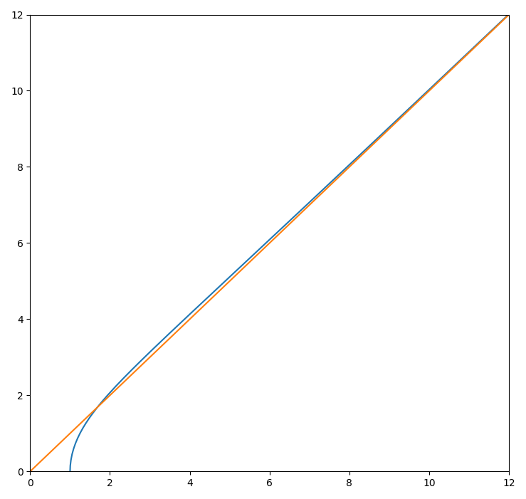
Note that the system is homogeneous of degree −1-1 meaning that if Γ⁡(s)\Gamma(s) is a solution, then for t>0t>0 the scaled version t−1​Γ​(t​s)t^{-1}\Gamma(ts) is also a solution. We solve this system numerically using the method odeint [14, 25] in the Scipy-Python software, which is based on the solver lsoda of the Fortran library ODEPACK and is used in the remaining examples too. The result is shown in Figure 3 left. Numerically we observe the following: Let Γ:[0,ℓ]→ℝ≥02\Gamma:[0,\ell]\to\mathbb{R}_{\geq 0}^{2} be a solution of (28) with initial conditions (27). Then for any t>0t>0 the domain

𝕏t:={Γ⁡(s)+u​N​(ζ⁡(s)):(s,u)∈(0,t)×ℝ}∩ℝ≥02\mathbb{X}_{t}:=\{\Gamma(s)+uN(\zeta(s)):(s,u)\in(0,t)\times\mathbb{R}\}\cap\mathbb{R}^{2}_{\geq 0}

is a rectangular triangle and Γ\Gamma is a principal curve for the uniform distribution on 𝕏t\mathbb{X}_{t}. Moreover, the angle ζ⁡(s)\zeta(s) oscillates around π4\frac{\pi}{4}, i.e, the function ζ⁡(s)−π4\zeta(s)-\frac{\pi}{4} has infinitely many zeros. In particular, this would imply that there are infinitely many closed principal curves for the square, see Figure 3 right, which converge to the trivial non-smooth solution.
Refer to caption
Refer to caption
Figure 3: Left: A solution to (28) with x1​(0)=1x_{1}(0)=1, x2​(0)=0x_{2}(0)=0, ζ⁡(0)=π2\zeta(0)=\frac{\pi}{2} (blue) and for comparison the diagonal (orange). Right: The derived non-trivial closed principal curve for the square (red) by composition of 8 identical principal curves on rectangular triangles. We show the normals (black) and the border of the projection domain.

5.3 Triangular-Based Prism

Let Δ⁡(E1,E2,E3)\Delta(E_{1},E_{2},E_{3}) be some triangle in the x1​x2x_{1}x_{2}-plane, and let

𝒫Δ:={𝒙∈ℝ3:(x1,x2,0)∈Δ(E1,E2,E3),x3∈[0,h]}\mathcal{P}_{\Delta}:=\{\bm{x}\in\mathbb{R}^{3}:(x_{1},x_{2},0)\in\Delta(E_{1},E_{2},E_{3}),x_{3}\in[0,h]\}

be the corresponding prism of height hh. We want to compute a principal curve starting at some point Γ⁡(0)∈Δ⁡(E1,E2,E3)\Gamma(0)\in\Delta(E_{1},E_{2},E_{3}) with tangent 𝜻⁡(0)=(π/2,π/2)\bm{\zeta}(0)=(\pi/2,\pi/2). If Γ\Gamma is admissible, then the cross-section between the prism and the normal planes at s∈(0,ℓΓ)s\in(0,\ell_{\Gamma}) are not allowed to intersect with the two bases of the prism. Therefore, the cross-sections are again triangles. To compute the vertices of this triangles within the normal coordinates, we may solve the equation systems

u1​N1​(𝜻⁡(s))+u2​N2​(𝜻⁡(s))−v​𝒆3=Ei−Γ⁡(s).u_{1}N_{1}(\bm{\zeta}(s))+u_{2}N_{2}(\bm{\zeta}(s))-v\bm{e}_{3}=E_{i}-\Gamma(s).

Notice that the system matrix [N1,N2,−e3][N_{1},N_{2},-e_{3}] is triangular, simplifying the computation of u1u_{1} and u2u_{2}. On the basis of these vertices, we may split the integration over u1u_{1} within the definition of the transverse moments into integrals of the form

μ~(j,k)​(s):=∫v1v2∫a+b​u1c+d​u1u1j​u2k​d​u2​d​u1.\tilde{\mu}_{(j,k)}(s):=\int_{v_{1}}^{v_{2}}\int_{a+bu_{1}}^{c+du_{1}}u_{1}^{j}u_{2}^{k}\,du_{2}\,du_{1}.

The required first and seconds transverse moments are thus summations about the partial moments

μ~(1,0)\displaystyle\tilde{\mu}_{(1,0)} =(d−b)3​(v23−v13)+(c−a)2​(v22−v12),\displaystyle=\frac{(d-b)}{3}\,(v_{2}^{3}-v_{1}^{3})+\frac{(c-a)}{2}\,(v_{2}^{2}-v_{1}^{2}),
μ~(2,0)\displaystyle\tilde{\mu}_{(2,0)} =(d−b)4​(v24−v14)+(c−a)3​(v23−v13),\displaystyle=\frac{(d-b)}{4}\,(v_{2}^{4}-v_{1}^{4})+\frac{(c-a)}{3}\,(v_{2}^{3}-v_{1}^{3}),
μ~(1,1)\displaystyle\tilde{\mu}_{(1,1)} =(d2−b2)8​(v24−v14)+(c​d−a​b)3​(v23−v13)+(c2−a2)4​(v22−v12),\displaystyle=\frac{(d^{2}-b^{2})}{8}\,(v_{2}^{4}-v_{1}^{4})+\frac{(cd-ab)}{3}\,(v_{2}^{3}-v_{1}^{3})+\frac{(c^{2}-a^{2})}{4}\,(v_{2}^{2}-v_{1}^{2}),
μ~(0,1)\displaystyle\tilde{\mu}_{(0,1)} =(d2−b2)6​(v23−v13)+(c​d−a​b)2​(v22−v12)+(c2−a2)2​(v2−v1),\displaystyle=\frac{(d^{2}-b^{2})}{6}\,(v_{2}^{3}-v_{1}^{3})+\frac{(cd-ab)}{2}\,(v_{2}^{2}-v_{1}^{2})+\frac{(c^{2}-a^{2})}{2}\,(v_{2}-v_{1}),
μ~(0,2)\displaystyle\tilde{\mu}_{(0,2)} =(d3−b3)12​(v24−v14)+(c​d2−a​b2)3​(v23−v13)\displaystyle=\frac{(d^{3}-b^{3})}{12}\,(v_{2}^{4}-v_{1}^{4})+\frac{(cd^{2}-ab^{2})}{3}\,(v_{2}^{3}-v_{1}^{3})
+(c2​d−a2​b)2​(v22−v12)+(c3−a3)3​(v2−v1).\displaystyle\qquad+\frac{(c^{2}d-a^{2}b)}{2}\,(v_{2}^{2}-v_{1}^{2})+\frac{(c^{3}-a^{3})}{3}\,(v_{2}-v_{1}).

Based on the moments, a principal curve of the triangular prism may be computed by solving the differential equation system. The results for a specific triangle are shown in Figure 4. The normal planes do here not intersect so that the solution curve is admissible. The computed curve coincides numerically with the curve through the means of the sections πΓ−1​([tk,tk+1])\pi_{\Gamma}^{-1}([t_{k},t_{k+1}]), where tkt_{k} corresponds to the time steps of the solution curve; so the solutions curve is self-consistent and hence a principal curve. Using the above procedure, we are able to compute principle curves of prism with arbitrary polygonal base.

Refer to caption
Figure 4: Principal curve in the triangular prism whose base corresponds to the points (0,1,0)(0,1,0), (3/2,−1/2,0)(\sqrt{3}/2,-1/2,0), (−2,−1/2,0)(-2,-1/2,0). The length of the prism is chosen such that both bases are parallel. The intersection of the normal planes 𝕏⁡(s)\mathbb{X}(s) with the surface of the prism are shown as red triangles. Since they do not intersect each other, the curve is admissible. The barycenters of the related Voronoi cells (green dots) numerically coincide with the curve. Note the scaling with respect to the x3x_{3}-axis.

5.4 Infinite Cylinder

The arclength parameterization of a helix Γ≡H\Gamma\equiv H is given by

H(s):=(a​cos⁡(k​s)a​sin⁡(k​s)b​k​s),k:=1/a2+b2,a,b>0.H(s):=\begin{pmatrix}a\cos(ks)\\ a\sin(ks)\\ bks\end{pmatrix},\qquad k:=1/\sqrt{a^{2}+b^{2}},\qquad a,b>0.

The corresponding Frenet frame reads as

T⁡(s)=(−a​k​sin⁡(k​s)a​k​cos⁡(k​s)b​k),N⁡(s)=(−cos⁡(k​s)−sin⁡(k​s)0),B⁡(s)=(b​k​sin⁡(k​s)−b​k​cos⁡(k​s)a​k)T(s)=\begin{pmatrix}-ak\sin(ks)\\ ak\cos(ks)\\ bk\end{pmatrix},\qquad N(s)=\begin{pmatrix}-\cos(ks)\\ -\sin(ks)\\ 0\end{pmatrix},\qquad B(s)=\begin{pmatrix}bk\sin(ks)\\ -bk\cos(ks)\\ ak\end{pmatrix}

Moreover, it has constant curvature κ\kappa and torsion τ\tau given by

κ=aa2+b2=a​k2,τ=ba2+b2=b​k2.\kappa=\frac{a}{a^{2}+b^{2}}=ak^{2},\qquad\tau=\frac{b}{a^{2}+b^{2}}=bk^{2}.

In what follows, we let

𝒞r:={(x1,x2,x3)T:x12+x22≤r2}\mathcal{C}_{r}:=\{(x_{1},x_{2},x_{3})^{\mathrm{T}}\;:\;x_{1}^{2}+x_{2}^{2}\leq r^{2}\}

be the infinitely long cylinder of radius rr. To find appropriate parameters, we consider (17). More precisely, we will compute the integral

H¯​(s)\displaystyle\bar{H}(s) :=As−1​∫πH−1​(s)(H⁡(s)+u1​N​(s)+u2​B​(s))​(1−u1​κ)​d​u1​d​u2,\displaystyle:=A_{s}^{-1}\int_{\pi_{H}^{-1}(s)}(H(s)+u_{1}N(s)+u_{2}B(s))(1-u_{1}\kappa)du_{1}du_{2},
As\displaystyle A_{s} :=∫πH−1​(s)(1−u1​κ)​d​u1​d​u2,\displaystyle:=\int_{\pi_{H}^{-1}(s)}(1-u_{1}\kappa)du_{1}du_{2},

whose value has to coincide with H⁡(s)H(s) if the helix is a principal curve, i.e. if (17) holds true. Without loss of generality we may assume s=0s=0 so that

H¯​(0)=H⁡(0)+u¯1​N​(0)+u¯2​B​(0)=(a00)+u¯1​(−100)+u¯2​(0−b​ka​k)\bar{H}(0)=H(0)+\bar{u}_{1}N(0)+\bar{u}_{2}B(0)=\begin{pmatrix}a\\ 0\\ 0\end{pmatrix}+\bar{u}_{1}\begin{pmatrix}-1\\ 0\\ 0\end{pmatrix}+\bar{u}_{2}\begin{pmatrix}0\\ -bk\\ ak\end{pmatrix}

where

u¯1\displaystyle\bar{u}_{1} :=A0−1∫ℰru1(1−κu1)du1du2,u¯2:=A0−1∫ℰru2(1−κu1)du1du2,\displaystyle:=A_{0}^{-1}\int_{\mathcal{E}_{r}}u_{1}(1-\kappa u_{1})du_{1}du_{2},\qquad\bar{u}_{2}:=A_{0}^{-1}\int_{\mathcal{E}_{r}}u_{2}(1-\kappa u_{1})du_{1}du_{2},
ℰr\displaystyle\mathcal{E}_{r} :={(u1,u2):(a−u1)2+(bku2)2≤r2},A0:=∫ℰr(1−κu1)du1du2.\displaystyle:=\{(u_{1},u_{2}):(a-u_{1})^{2}+(bku_{2})^{2}\leq r^{2}\},\qquad A_{0}:=\int_{\mathcal{E}_{r}}(1-\kappa u_{1})du_{1}du_{2}.

Straightforward calculation leads to

u¯1=a⁡(1−r24​b2),u¯2=0\bar{u}_{1}=a\left(1-\frac{r^{2}}{4b^{2}}\right),\qquad\bar{u}_{2}=0

such that

H¯​(0)=(a​r2/(4​b2),0,0)T.\bar{H}(0)=\big(ar^{2}/(4b^{2}),0,0\big)^{\mathrm{T}}.

Setting H¯​(0)\bar{H}(0) equal to H⁡(0)H(0) and imposing the non-negativity of the Jacobian determinant, i.e. κ​u1≤1\kappa u_{1}\leq 1, (u1,u2)∈ℰr(u_{1},u_{2})\in\mathcal{E}_{r}, we infer that the helix is a principal curve for the uniform measure of the cylinder 𝒞r\mathcal{C}_{r} if

b=r/2,0≤a≤r/4.b=r/2,\qquad 0\leq a\leq r/4.

Numerical experiments indicate that for r/4<a<2​r/3r/4<a<2r/3 there exists b<r/2b<r/2 such that the helix is also a principal curve, see Figure 5. Note the limiting case b=0b=0 and a=2/3a=2/3, where the helix degenerates to a circle. However, in these cases the helix has points of ambiguity inside the cylinder.

Refer to caption
Refer to caption
Refer to caption
Figure 5: Helices for several parameters (a,b)∈{(0.2,0.5),(0.6,0.35),(0.66,0.1)}(a,b)\in\{(0.2,0.5),(0.6,0.35),(0.66,0.1)\} (from top to bottom). The curves are sampled equidistantly (blue dots). For some sampling points the Voronoi regions intersected with the cylinder of radius r=1r=1 are depicted in golden color. Note that for the second and third set of parameters the helices are not admissible curves for the infinite cylinder.

6 Conclusion

We have derived a dynamical system for finding principal curves of random variables in ℝd\mathbb{R}^{d} for d≥2d\geq 2 and have numerically computed the solution for uniformly distributed random variables with density functions supported on certain domains. It will be of interest to consider also other distributions as, e.g. Gaussian mixtures. Another issue would be to have a look at principle curves on manifolds as started in the papers [13, 17].

Further, so far only the squared Euclidean norm was incorporated into the considerations. Unfortunately, classical PCA based on this ,,distance” is sensitive to outliers so that robust methods were considered in the literature, e.g. by skipping the square in the Euclidean norm or taking the Ł1\L_{1} norm. For an overview of robust subspace recovery, we refer to [21] and the references therein and to recent results on robust principal lines [22]. So far we are not aware of a robust principal curve approach.

Acknowledgement: Funding by the DFG under Germany’s Excellence Strategy – The Berlin Mathematics Research Center MATH+ (EXC-2046/1, Projektnummer: 390685689) is acknowledged.

References

  • [1] J. Banfield and A. Raftery. Ice floe identification in satellite images using mathematical morphology and clustering about principal curves. J. Am. Stat. Assoc., 87:7–16, 1992.
  • [2] R. L. Bishop. There is more than one way to frame a curve. Am. Math. Mon., 82(3):246–251, 1975.
  • [3] K.-y. Chang and J. Ghosh. Principal curves for nonlinear feature extraction and classification. Appl. Artif. Neural Netw. Image Process. III, 3307:120–129, 1998.
  • [4] D. Chen, J. Yin, S. Yang, L. Li, and P. Pudney. Constraint local principal curve: concept, algorithms and applications. J. Comput. Appl. Math., 298:222–235, 2016.
  • [5] F. de Gournay, J. Kahn, and L. Lebrat. Differentiation and regularity of semi-discrete optimal transport with respect to parameters of the discrete measure. Numer. Math., 141:429–453, 2019.
  • [6] P. Delicado. Another look at principal curves and surfaces. J. Multivar. Anal., 77(1):84–116, 2001.
  • [7] D. Dong and T. J. McAvoy. Nonlinear principal component analysis - based on principal curves and neural networks. Comput. Chem. Eng., 20(1):65–78, 1996.
  • [8] T. Duchamp and W. Stuetzle. The geometry of principal curves in the plane. Technical Report 250, Department of Statistics, GN-22, University of Washington, Seattle, February 1993.
  • [9] T. Duchamp and W. Stuetzle. Extremal properties of principial curves in the plane. Ann. Stat., 24(4):1520, 1996.
  • [10] M. Ehler, M. Gräf, S. Neumayer, and G. Steidl. Curve based approximation of measures on manifolds by discrepancy minimization. Found. Comput. Math., accepted.
  • [11] T. Hastie. Principal curves and surfaces. Technical report, PhD Thesis, Stanford University, 1984.
  • [12] T. Hastie and W. Stuetzle. Principal curves. J. Am. Stat. Assoc., 84(406):502–516, 1989.
  • [13] S. Hauberg. Principal curves on Riemannian manifolds. IEEE Trans. Pattern Anal. Mach. Intell., 38(9):1915–1921, 2016.
  • [14] A. C. Hindmarsh. Odepack: A systematized collection of ODE solvers. In Sci. Comput., volume 1 of IMACS Trans. Sci. Comput., pages 55–64. North-Holland, Amsterdam, 1983.
  • [15] T. Huckemann, S. Hotz, and A. Munk. Intrinsic shape analysis: geodesic principle component analysis for Riemannian manifolds modulo Lie group actions. Stat Sin., 20:1–100, 2010.
  • [16] B. Kégl. Principal curves: learning, design, and applications. PhD thesis, 1999.
  • [17] J. H. Kim, J. Lee, and H. S. Oh. Spherical principal curves. ArXiv Preprint, 2003.02578, 2020.
  • [18] A. Klenke. Probability Theory. Universitext. Springer, Cham, 3rd edition, 2020.
  • [19] A. Krzyzak, B. Kégl, T. Linder, and K. Zeger. Learning and Design of Principal Curves. IEEE Trans. Pattern Anal. Mach. Intell., 22(3):281–297, 2000.
  • [20] L. Lebrat, F. de Gournay, J. Kahn, and P. Weiss. Optimal transport approximation of 2-dimensional measures. SIAM J. Imaging Sci., 12(2):762–787, 2019.
  • [21] G. Lerman and T. Maunu. An overview of robust subspace recovery. Proc. IEEE, 106(8):1380–1410, 2018.
  • [22] S. Neumayer, M. Nimmer, S. Setzer, and G. Steidl. On the robust PCA and Weiszfeld’s algorithm. Appl. Math. Optim., 82:1017–1048, 2019.
  • [23] K. Pearson. On lines and planes of closest fit to systems of points in space. Philos. Mag., 2(11):559–572, 1901.
  • [24] X. Pennec. Barycentric subspaces and affine spans in manifolds. Int. Conf. Netw. Geom. Sci. Inform., pages 12–21, 2015.
  • [25] L. Petzold. Automatic selection of methods for solving stiff and non-stiff systems of ordinary differential equations. SIAM J. Sci. Statist. Comput., 4(1):136–148, 1983.
  • [26] K. Reinhard and M. Niranjan. Subspace Models For Speech Transitions Using Principal Curves. Proc. Inst. Acoust., 20:53–60, 1998.
  • [27] S. Sommer, F. Lauze, and M. Nielsen. Optimization over geodesics for exact principle geodesic analysis. Adv. Comput. Math., 40:283–313, 2013.
  • [28] P. Thomas Fletcher. Geodesic regression and the theory of least squares on Riemannian manifold. Int. J. Comput. Vis., 105:171–185, 2013.
  • [29] S. Yılmaz and M. Turgut. A new version of Bishop frame and an application to spherical images. J. Math. Anal. Appl., 371(2):764–776, 2010.