Manifold-Inspired Single Image Interpolation

We remove aliasing in high frequencies via applying Gaussian low-pass filtering to $\bm{I}_{L}$:

where $\ast$ denotes the convolution operator. The filter $\bm{F}$, of size $d\times d$, is a unit-gain, 2D Gaussian with standard deviation $\sigma$.

Low-pass filtering with a fixed blur kernel can only handle mild aliasing. When aliasing is so strong that corrupts the low-frequency components, typical structures such as the originally continuous spokes in Fig. 2 (a) turn discontinuous in Fig. 2 (b). Applying spatially-invariant low-pass filtering on the input image can hardly recover the continuity since the low frequency components have already been corrupted. In Fig. 2 (c), the target patch containing disjointed spokes can hardly find its similar patches containing a continuous piece of spoke. Thus, the spokes in the refined target patch will often remain disjoint, which severely affects the visual perception.

The regions with strong aliasing often contain directional localized structures. Preserving the orientations of these structures is the key to preserving the continuity and to identifying reliable similar patches. This motivates us to design an adaptive operator to extract the orientation-related characterizations of each patch and to represent the patch by such characterizations. Principal components of a group of similar patches in the vicinity of directional structures are such characterizations, since for a few bases to capture the vast majority of the energy of these patches, their manifested directions shall be aligned with the directions of the localized structure.

To robustly estimate the bases, the influence of aliasing in $\bm{I}_{L}^{lp}$ shall be attenuated. Here we borrow the idea of denoising by averaging. Specifically, when computing the principal components, instead of using a group of patches similar to the $i$-th target patch, $\bm{P}^{lp}_{i}$, from $\bm{I}_{L}^{lp}$, we use the union of groups of patches. Each group of $K_{ar}$ patches is similar to one of the $9$ patches within the $3\times 3$ neighborhood of $\bm{P}^{lp}_{i}$’s position. The reason why involving the union of $9$ groups of patches can attenuate aliasing is that the aliasing components are often distinct at $9$ positions yet the orientations are nearly identical. For notational convenience, we denote the union of grouped matrix as $\bm{Y}_{i}$, of size $\tilde{K}\times n^{2}$, where $\tilde{K}$ is the cardinality of the union of the $9$ sets and $n$ is the patch’s size length. We also denote its centered version as $\tilde{\bm{Y}}_{i}$, so that

where each row of $\bar{\bm{Y}}_{i}$, $\bar{\bm{y}}_{i}^{\top}$, is the mean of $\tilde{K}$ patches. In addition, we denote $\tilde{\bm{y}}_{i}\in\mathbb{R}^{n^{2}\times 1}$ as:

Given $\tilde{\bm{Y}}_{i}$, we solve for its top $k$ principal components through SVD in order for them to represent the local directions. $\tilde{\bm{Y}}_{i}$ is decomposed as:

where $\bm{U}_{i}$ is a $\tilde{K}\times\tilde{K}$ unitary matrix; $\bm{D}_{i}$ is a $\tilde{K}\times n^{2}$ diagonal matrix with non-negative real numbers on the diagonal; $\bm{V}_{i}$ is a $n^{2}\times n^{2}$ unitary matrix. The $j$-th columns of $\bm{V}_{i}$ is denoted as as $\bm{v}^{j}_{i}$, where $1\leqslant j\leqslant k$. Aiming to preserve the directional structures, we update $\tilde{\bm{y}}_{i}$ as $\tilde{\bm{y}}^{u}_{i}$, the linear combination only of the top $k$ principal components through:

By averaging the contribution of all the overlapped updated target patches relevant to each pixel, we generate an intermediate version of aliasing-removed image via:

where $\hat{\bm{P}}_{i}=\tilde{\bm{y}}^{u}_{i}+\bar{\bm{y}}_{i}$; $l$ is the number of target patches in $\bm{I}_{L}^{lp}$; $\bm{R}_{i}(\cdot)$ is an operator extracting $n^{2}$ pixels from the $i$-th patch from an image; $\bm{R}^{\top}_{i}(\cdot)$ puts back $n^{2}$ pixels into the $i$-th position and padds with zeros elsewhere; $./$ stands for the element-wise division of two matrices; $\bm{1}_{n^{2}\times 1}$ is a vector of size $n^{2}\times 1$ with all the elements being $1$.

By repeating the above procedures for another time and applying bicubic interpolation to the output computed from (6), we generate $\bm{{I}}_{ar}$ as the image with removed aliasing in low and high frequencies of the same size as the HR image. A typical example of $\bm{{I}}_{ar}$ is illustrated in Fig. 2(d) where the spokes retain the smoothness in the original HR image. $\bm{{I}}_{ar}$ well preserves the dominant directions of localized edges but removes the secondary directions of localized edges. We will further refine $\bm{{I}}_{ar}$ in Section IV-A to better estimate the similar patches in the vicinity of localized edges along secondary directions. Prior to generating the refined version of $\bm{{I}}_{ar}$, $\bm{{I}}_{ar}$ will first serve as a preliminary aliasing-removed image to initialize the selection of similar patches and to estimate the weights of similar patches in Section III.

We assume the low-resolution input image $\bm{I_{L}}$ of size $M\times N$ to be the directly downsampled version of a high-resolution image $\bm{I_{H}}$ of size $2M\times 2N$. The downsampling grid starts with the upper-left pixel in $\bm{I_{H}}$, i.e.

where $1\leqslant p\leqslant M,1\leqslant q\leqslant N$. The interpolated image is labeled as $\bm{\hat{I}_{H}}$ which aims to be as close to $\bm{I_{H}}$ as possible. In the iterations to generate $\bm{\hat{I}_{H}}$ from $\bm{I_{L}}$, there exists an unrefined target patch with even side length $n$. We label the $i$-th unrefined target patch as $\bm{P}_{i}~(\bm{P}_{i}\in\mathbb{R}^{n^{2}\times 1})$.

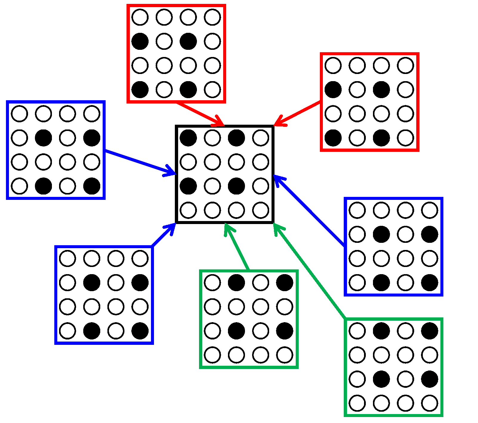
For notational convenience, we categorize the pixels in $\bm{I_{H}}$ as OO-, OE-, EO-, EE-located, depending on the parity (O stands for odd, E stands for even) of its vertical and horizontal coordinates. As mentioned in (7), the measured pixels are OO-located. In addition, we denote the patches with its upper-left pixels be OO-, OE-, EO-, EE-located as OO, OE, EO, EE patches. Regarding each patch as a $n\times n$ image whose upper-left pixel’s vertical and horizontal coordinates are both odd, we categorize OO-, OE-, EO-, EE-located pixels within a patch as OO-, EO-, OE-, EE-phase pixels. Assuming each target patch is OO-located, as illustrated in Fig. 3, among all similar patches, OE, EO, EE patches will have OE-, EO-, EE-phase pixels(all measured pixels) similar to unrefined OE-, EO-, EE-phase pixels in the target patch, respectively. In other words, all the unrefined pixels in a target patch have their similar pixels found as the measured pixels. To estimate the target patch’s unrefined pixels (OE-, EO-, EE-phase pixels), we use their corresponding measured pixels from OE, EO, EE similar patches as bases and express the refined target patch as:

where $\hat{\bm{P}}_{i}$, $\bm{P}_{i,j}^{OE}$, $\bm{P}_{i,j}^{EO}$, $\bm{P}_{i,j}^{EE}$ $\in$ $\mathbb{R}^{n^{2}\times 1}$ are the vectorized forms of the refined target patch, the target patch’s $j$-th similar OE, EO and EE patches, respectively; $\omega_{i,j}^{OE}$, $\omega_{i,j}^{EO}$, $\omega_{i,j}^{EE}$ are the weights of $j$-th similar OE, EO, EE patch of $\bm{P}_{i}$, respectively; each type of similar patches has $K^{OE}$, $K^{EO}$, $K^{EE}$ patches, respectively; $\bm{M}^{OO}$, $\bm{M}^{OE}$, $\bm{M}^{EO}$, $\bm{M}^{EE}$ $\in$ $\mathbb{R}^{n^{2}\times n^{2}}$ are matrices that select OO-, OE-, EO-, EE-phase pixels from a patch and sets the rest of pixels $0$. After updating each target patch, we average all target patches and generate the refined image via (6) (here $l$ refers to the number of OO patches).

Mitigating the influence of aliasing on estimating the refined patches is the key task in the initial iteration. We use the measured pixels from similar patches as the bases and estimate their weights using patches from an aliasing-removed image.

In the initial iteration, we denote the aliasing-removed image as $\bm{I}_{G}$ and use $\bm{I}_{G}$ (guide image) to search the positions of similar patches of each target patch and to compute their corresponding weights for estimating the target patch. Specifically, similar patches are searched in a $W\times W$ ($W$ is odd) square window centered at the target patch’s upper-left pixel coordinate. The similarity metric is defined as:

where $\bm{P}^{G}_{i}$ denotes the $i$-th patch in $\bm{I}_{G}$ sharing the same position of the unrefined $i$-th target patch $\bm{P}_{i}$; $\bm{P}^{Gf}_{i,j}$ denotes the $j$-th patch within the neighorhood of $\bm{P}^{G}_{i}$ belonging to OE (f refers to OE), EO (f refers to EO) or EE (f refers to EE) patches; $\|\bm{P}^{G}_{i}-\bm{P}^{Gf}_{i,j}\|_{1}$ denotes the $\ell_{1}$ distance between two patches in $\bm{I}_{G}$; and $c_{w}$ is a constant that controls the decay of similarity values as a function of the $\ell_{1}$ distance. For OE, EO or EE similar patches, the similarity values of top $K^{f}$ similar patches are stored in descending order in vector $\bm{S}_{i}^{OE}$, $\bm{S}_{i}^{EO}$ and $\bm{S}_{i}^{EE}$, respectively.

Given the positions of $\bm{P}_{i}$’s similar patches at each phase, the weights of these similar patches ($\bm{\omega}_{i}^{f}$) are computed by approximating the OO-phase pixels in $\bm{P}^{G}_{i}$ via their corresponding OO-phase pixels from similar patches. The reason we only use OO-phase pixels here is because in early iterations, the pixels on measurement grid are more reliable than the pixels off the measurement grid. $\bm{\omega}_{i}^{f}$ is computed with a closed-form solution by solving a regularized least squares problem:

where $\bm{Q}^{f}_{i}$, of size $n^{2}\times K^{f}$, stores one type (OE, EO or EE) of top-$K^{f}$ similar patches; $\bm{M}_{c}^{OO}$ is a $\frac{n^{2}}{4}\times n^{2}$ matrix that selects OO-phase pixels; $\lambda$ is a scalar that controls the regularization strength; $\bm{\Sigma}^{f}_{i}=\mathop{\rm diag}\left(\frac{{\bm{S}^{f}(1)}}{{\bm{S}^{f}(1)}},\dots,\frac{{\bm{S}^{f}(1)}}{{\bm{S}^{f}(i)}},\dots,\frac{{\bm{S}^{f}(1)}}{{\bm{S}^{f}(K)}}\right)$ is a diagonal matrix that penalizes the weights of less similar patches. Given (10), (8), we compute a refined patch $\hat{\bm{P}}_{i}$. By averaging all the refined patches, we generate an intermediately interpolated image via (6).

The interpolated image from the initial iteration is coarsely estimated since both the collected similar patches and their weights are determined by $\bm{I}_{G}$ which has few high-frequency details. To refine the coarsely interpolated image, we treat the previously interpolated image as $\bm{I}_{G}$ to identify similar patches and compute their weights in the next iteration and to use a smaller patch size. By several iterations, we generate the output image $\bm{I}_{\mathrm{S1}}$ from Stage $1$B with its details in Algorithm 2. Due to the similarity between the initial iteration (Stage $1$A) and the follow-up iterations (Stage $1$B), we name these iterations as Stage $1$. Owing to significance of the initial iteration (Stage $1$A), we will further discuss it in Section V-A.

The major drawback of Stage $1$ is that estimating the weights of similar patches is imprecise: only a quarter of pixels are used in the target patch and similar patches. In Stage $2$, we estimate the weights by involving all the pixels in similar patches to approximate all the pixels in the target patch. The weights $\bm{\omega}^{f}_{i}$ is solved via:

where the notations are identical to those in (10). By several iterations, we obtain the output image $\bm{I}_{\mathrm{S2}}$ from Stage $2$. The details of Stage $2$ is described in Algorithm 3.

The major drawback of Stage $1$ and Stage $2$ is that for each target patch, only OE, EO and EE similar patches are used and OO similar patches are ignored. To address the drawback, Stage $4$ exploits OO similar patches to refine the pixels off the measurement grid in each target patch since these pixels are close to ground-truth after iterations in the previous two stages. Thus, we approximate each target patch as a linear combination of all the similar patches regardless of OO, OE, EO or EE patches. Further, the target patch is not limited to a OO patch, but can be any OO, OE, EO, EE patch.

Mathematically, we use a target patch and its similar patches ($K$ patches in total) to approximate the target patch itself. The similar patches is searched based on a new similarity metric:

The motivation of the new similarity metric is to involve correlated patches as the similar patches. It is likely that the patches of the edges along the same directions, of the same sharpness, but with different polarities can be considered as the same patch. Prior to computing the similarity metric, we subtract the input image by the mean of the measured pixel values to involve similar patches with different polarities.

The weights of $K$ patches, $\bm{\omega}_{i}$, is computed via:,

where $\bm{Q}_{i}$ refers to the matrix of size $n^{2}\times K$ that stores all the $K$ patches; $\bm{\Sigma}_{i}=\mathop{\rm diag}\left(\frac{{\bm{S}(1)}}{{\bm{S}(1)}},\dots,\frac{{\bm{S}(1)}}{{\bm{S}(i)}},\dots,\frac{{\bm{S}(1)}}{{\bm{S}(K)}}\right)$ is a diagonal matrix that penalizes the weights of less similar patches in $\bm{I}_{G}$. Given $\bm{\omega}_{i}$, the updated patch $\hat{\bm{P}}_{i}$ is solved by:

where $\bm{M}^{r}=\bm{M}^{OE}+\bm{M}^{EO}+\bm{M}^{EE}$; $\omega_{i,j}$ is a scalar that denotes the weight of $j$-th similar patch of $\bm{P}^{G}_{i}$. After synthesizing all updated patches, we obtain a new image and complete one iteration. After a few iterations, we add the aforementioned mean and obtain the output image with the details shown in Algorithm 4. Note that we choose a smaller patch size ($n_{B}<n_{A}$) after $i_{A}$ iterations in Algorithm 4 to exploit semi-local similarity at a finer scale.

In previous stages, our approach to estimating the weights of less similar patches is ad-hoc: we simply assign smaller weights. To better handle less similar patches, we consider a similar patch as a combination of similar and dissimilar structures to the target patch. Dissimilar structures may include mild aliasing pattern distinct from the target patch and shall capture a smaller portion of energy compared with similar structures among the group of similar patches and the target patch. This motivates us to represent the group of patches via a few bases by applying SVD to the group while only preserving dominant principal components. We denote the group corresponding to the $i$-th target patch as $\bm{X}_{i}\in\mathbb{R}^{k\times n^{2}}$ with $k$ patches and each patch is stored as a row with $n^{2}$ pixels. Also we denote the centered version of $\bm{X}_{i}$ as $\tilde{\bm{X}}_{i}$. $\tilde{\bm{X}}_{i}=\bm{X}_{i}-\bar{\bm{X}}_{i}$, where each row of $\bar{\bm{X}}_{i}$ is the mean of $k$ patches. We also denote the target group as $\tilde{\bm{X}}^{lr}_{i}$. $\tilde{\bm{X}}^{lr}_{i}$ is spanned by only a few principal components and can be computed via low-rank approximation.

Noticing that a principal component corresponding to a larger singular value carries fewer dissimilar structures than a principal component corresponding to a smaller singular value does, we choose to less shrink a larger singular value and more shrink a smaller singular value. Thus, we use the Weighted Nuclear Norm Minimization (WNNM) [15] as below:

where $\sigma_{j}(\tilde{\bm{X}}^{lr}_{i})$ is the $j$-th singular value of $\tilde{\bm{X}}^{lr}_{i}$; $\omega_{j}$ is the weight on the $j$-th singular value; $\alpha$ is a parameter that controls the regularization strength. Since a larger singular values deserves less shrinkage, we choose a smaller weight. As mentioned in [16], we the empirical distribution of singular values can be modeled as a Laplacian. Given this prior and inspired by BayesShrink in [17], we choose the threshold as:

where $\omega_{j}$ is the weight corresponding to the $j$-th singular value of $\tilde{\bm{X}}^{lr}_{i}$; $\hat{\sigma}_{j}=\sqrt{(\sigma_{j}(\tilde{\bm{X}}^{lr}_{i})^{2}/n^{2})}$ is the estimation of signal standard deviation given the $i$-th singular value; $\epsilon$ is a small constant. Based on [15], the solution of (15) is:

where $\bm{U}_{i}\bm{D}_{i}\bm{V}_{i}^{\top}=\tilde{\bm{X}}_{i}$ and ${\mathcal{S}}_{\bm{\omega}_{i}}$ is the generalized soft-thresholding operator with the weighted vector ${\bm{\omega}_{i}}$ as the threshold to threshold the diagonal elements of $\bm{D}_{i}$, i.e. $\left[{\mathcal{S}}_{\bm{\omega}_{i}}(\bm{D}_{i})\right]_{j,j}=\max(\left[\bm{D}_{i}\right]_{j,j}-\alpha\omega_{j},0)$.

The estimated image will be computed via averaging the contribution of relevant groups of patches to each pixel:

where $\bm{R}_{G_{i}}(\cdot)$ extracts the group of $k$ patches corresponding to the $i$-th target patch; $\bm{R}^{\top}_{G_{i}}(\cdot)$ puts back the $i$-th group of patches into their original positions and pads with zeros elsewhere; $./$ stands for element-wise division of two matrices; $l$ is the number of grouped patches in the input image; $\bm{1}_{n^{2}\times k}$ is a matrix of size $n^{2}\times k$ with all the elements being $1$. After multiple iterations, we generate the output image from Stage $4$. The details of Stage $4$ are in Algorithm 5.

Since the spatially-variant projection in Algorithm 1 discards the energy spanned by less dominant components, the less dominant directional features will be removed when secondary edges carry distinct directions to directions of the dominant edges. We denote the phenomenon as the bias towards dominant edges and demonstrate it in Fig. 5(b). The original local directions (the red arrows in Fig. 5(a)) whose directions are drastically different from the dominant directions (the green arrows in Fig. 5(a)) become invisible in Fig. 5(b). Using Fig. 5(b) as the guide image will result to wrong similar patches and subsequently gives rise to visual artifacts in the interpolated images. Fig. 5(c) demonstrates such artifacts in the interpolated image through Stage $1-4$ by treating $\bm{I}_{ar}$ as the guide image $\bm{I}_{G}$ in Fig. 4.

To address this bias, we first use $\bm{I}_{ar}$ as the preliminary guide image to generate an interpolated image, blur the interpolated image, and then use the blurred image as a refined guide image to regenerate the interpolated image. The rationale behind this blur operator is that the pixels in the vicinity of removed directional features often carry very high frequency (shown in Fig. 5(c)), due to the difference between the interpolated dominant directions and the secondary directions formed by the measured pixels at the downsampling grid.

The scheme to handle the bias is shown in Fig. 6. This scheme follows the idea described in the above paragraph but with one more interpolation procedure to more robustly generate the guide image $\bm{I}_{G}$. We treat $\bm{I}_{G}$ from Fig. 6 as the guide image to guide the initial iteration in Fig. 4.

The scheme of interpolating by a factor of $3$ is mostly analogous to that of interpolating by a factor of $2$ in Fig. 4, except that the scheme of interpolating by a factor of $3$ discards Stage $4$ and only uses Stage $1-3$. The rationale behind not using Stage $4$ is that, the input LR image downsampled by a factor of $3$ from the original HR image is severely aliased and our interpolation algorithm may select wrong similar patches. The performance drop due to “refining” the regions with wrong similar patches generally outweighs the gain due to refining the regions with reliable similar patches.

We conducted the following ablation studies to access the importance of various features of MISTER. This study records the stage-wise $\mathrm{PSNR}$ evolution for MISTER and the $\mathrm{PSNR}$ of final results of four controlled experiments. We first describe the four controlled experiments, and explain the motivation for each of them. Finally, we present and discuss the results.

• •

  The first controlled experiment (E-C1) uses the bicubic interpolated version of $\bm{I}_{L}$ as the guide image $\bm{I}_{G}$ in Fig. 4. This guide image will be utilized to initialize the selection of similar patches and to compute the weights of similar patches in Stage $1$A;

• •

  The second controlled experiment (E-C2) uses $\bm{I}_{G}$ computed from the scheme in Fig. 6 as the guide image $\bm{I}_{G}$ in Fig. 4. This guide image will be used only to initialize the selection of similar patches. Given these selected similar patches, we use the bicubic interpolated version of $\bm{I}_{L}$ to compute the weights of similar patches in Stage $1$A;

• •

  The third controlled experiment (E-C3) uses the bicubic interpolated version of $\bm{I}_{L}^{lp}$ computed from (1) with fine-tuned filter parameters as the guide image $\bm{I}_{G}$ in Fig. 4. This guide image will be utilized to initialize the selection of similar patches and to compute the weights of similar patches in Stage $1$A;

• •

  The fourth controlled experiment (E-C4) uses $\bm{I}_{ar}$ computed from Algorithm 1 as the guide image $\bm{I}_{G}$ in Fig. 4. This guide image will be utilized to initialize the selection of similar patches and to compute the weights of similar patches in Stage $1$A.

E-C1 highlights the combined influence of aliasing both on choosing reliable similar patches and on estimating the weights of similar patches in the final result. The guide image of the initial iteration in E-C1 is significantly more aliased than that of MISTER. E-C2 isolates the influence of aliasing on estimation of the weights of similar patches in the final result. The initial iteration of E-C2 uses the same initial set of similar patches as MISTER does but uses the aliased pixels to estimate the weights. E-C3 highlights the influence of aliasing in the low-frequency components on the final result. E-C3 uses a guide image in the initial iteration with aliasing removed from its high-frequency components, but with significantly more low-frequency aliasing compared with MISTER. E-C4 examines the influence of the bias towards the dominant edges in removing aliasing on the final result. E-C4 uses $\bm{I}_{ar}$ as the guide image in the initial iteration, with fewer secondary edges compared with MISTER. For MISTER, E-C1, E-C2, E-C3 and E-C4, we show their $\mathrm{PSNR}$ evolution by stage in Table I.

Comparing the E-C1 row with the MISTER row in Table I, we find that the combined effect of the initial aliasing is substantial. The E-C1 $\mathrm{PSNR}$ in the final result drops from the MISTER $\mathrm{PSNR}$ both by $0.48$ dB for the tasks of interpolating by a factor of $2$ and $3$. Comparing the E-C2 row of Table I to the MISTER row, we find that the effect of aliasing isolated to the estimation of weights is also quite significant. After all iterations, E-C2’s $\mathrm{PSNR}$ drops from MISTER by $0.37$ dB and by $0.12$ dB in the tasks of interpolating by a factor of $2$ and $3$, respectively. Comparing the E-C3 row with the MISTER row in Table I, we find that the aliasing in the low-frequency components has a non-trivial influence on the final result. After all iterations, E-C3’s $\mathrm{PSNR}$ drops from MISTER by $0.16$ dB and by $0.23$ dB in the task of interpolating by a factor of $2$ and $3$, respectively. Comparing the E-C4 row with the MISTER row in Table I, we find that the bias towards dominant edges in removing aliasing has a non-trivial influence on the final result. E-C4’s $\mathrm{PSNR}$ after all the iteration drops from MISTER by $0.10$ dB and by $0.15$ dB in the tasks of interpolating by a factor of $2$ and $3$, respectively.

In addition to studying the aforementioned features, we explore the significance of the refinement after the first iteration, i.e. the combination of Stage $1$B, Stage $2$, Stage $3$, Stage $4$. This refinement process in MISTER offers $0.50$ dB and $0.32$ dB $\mathrm{PSNR}$ gains in the task of interpolating by a factor of $2$ and $3$, respectively. Each of those stages in the interpolation by a factor of $2$ task offers an non-trivial $\mathrm{PSNR}$ gain. Similarly, in the interpolation by a factor of $3$ task, those stages are trending to improve the $\mathrm{PSNR}$.

In conclusion, each of the features of MISTER, i.e. i) removing the aliasing in the low-frequency components; ii) mitigating the bias towards dominant edges in removing aliasing; iii) using aliasing-removed image to guide the selection of similar patches in the initial iteration; iv) using aliasing-removed image to compute the weights of similar patches in the initial iteration; and v) the sequential use of the manifold models for exploiting semi-local similarity, plays a significant role in achieving the interpolation quality of MISTER.

For the task of interpolating by a factor of $2$, in Table II, we compare MISTER with related works. These methods include (i) bicubic interpolation (Bicubic) (ii) New Edge-Directed Interpolation (NEDI) [3], (iii) Sparse Mixing Estimation (SME) [5], (iv) Soft-Decision and Adaptive Interpolator (SAI) [4], (v) Regularized Local Linear Regression (RLLR) [6], (vi) Multiscale Semilocal Interpolation with Antialiasing (MSIA) [8], (vii) Nonlocal Geometric Similarities and Directional Gradients (NGSDG) [11], (viii) Nonlocal Auto-Regressive Modeling (NARM) [9], (ix) Adaptive Non-local Sparsity Modeling (ANSM) [10], (x) Non-Local Patch Collaging (NLPC) [12], (xi) Fast Image Interpolation via Random Forests (FIRF) [19] and (xii) Multi-scale Attention-aware Inception Network (MAIN) [20]. Note that FIRF and MAIN are data-driven, learning-based approaches that learn the model parameters from an external set of training images. FIRF exploits random forests to partition the space of patches into subspaces and trains a regression model for each subspace to compute the HR image’s patches from their counterparts in the LR image. MAIN uses deep learning based, attention-aware inception (AIN) networks to interpolate images and fuse the interpolated images from multi scales to generate the output image. Involving FIRF and MAIN is to explore the performance difference between model-based approaches and data-driven, learning-based approaches. Table II demonstrates that compared with model-based algorithms, MISTER achieves the highest average $\mathrm{PSNR}$ and the highest $\mathrm{PSNR}$ in all the $27$ images. Specifically, compared with patch-based methods [9, 10, 12], MISTER has an average $\mathrm{PSNR}$ that is $0.97$ dB better than NARM, $0.61$ dB better than ANSM and $0.72$ dB better than NLPC. MISTER outperforms NEDI, SME, SAI, RLLR, MSIA, NGSDG and bicubic interpolation with an average gain of $1.83$ dB, $1.34$ dB, $1.29$ dB, $1.32$ dB, $1.31$ dB, $1.38$ dB and $2.20$ dB, respectively. Compared with FIRF and MAIN, MISTER’s average $\mathrm{PSNR}$ is higher than FIRF by $0.51$ dB, but lower than MAIN by $0.92$ dB.

Fig. 8, 9, 10 demonstrate visual comparisons between the above algorithms’ results. In Fig. 8(n), MISTER’s edges along upper-left to bottom-right orientation preserve both smoothness along the contour direction and sharpness across the profile direction, without noticeable artifacts. Among the interpolated edges from model-based methods, the edges from ANSM have the most similar visual quality to ours, but with noticeable jaggies along the contour direction. In Fig. 9(n), MISTER’s textures preserve the correct directions (from upper-left to bottom-right) as the ground-truth image. However, the textures from the other model-based algorithms generates distinctly different directions from the ground-truth. In Fig. 10(n), MISTER’s edges preserve the contour continuity of all the spokes along various directions. Among the interpolated edges from all the model-based algorithms, the edges from ANSM and MSIA have the most similar visual quality to ours. Yet, MSIA’s spokes exhibit zipper artifacts and jaggies and ANSM’s spokes exhibit mild but noticeable jaggies.

It is interesting that although FIRF achieves higher $\mathrm{PSNR}$ than recent model-based single image interpolation algorithms, strong artifacts are noticeable from Fig. 8(l), 9(l), 10(l). For example, the contours along upper-left to bottom-right directions are not smooth in Fig. 8(l) and Fig. 10(l). The directions of the textures in Fig. 9(l) are hardly noticeable.

For the task of interpolation by a factor of $3$, due to the availability of the source code, we compare MISTER only with bicubic interpolation, NARM, ANSM, NLPC and MAIN in Table III. Table III demonstrates that among model-based single image interpolation algorithms, MISTER achieves the highest average $\mathrm{PSNR}$ and the highest $\mathrm{PSNR}$ in $25$ out of $27$ images. Specifically, MISTER outperforms bicubic interpolation, NARM, ANSM and NLPC with an average $\mathrm{PSNR}$ improvement of $1.74$ dB, $0.96$ dB, $0.65$ dB and $0.54$ dB, respectively. Compared with the deep-learning based MAIN, MISTER’s average $\mathrm{PSNR}$ is $0.92$ dB lower.

We exhibit the visual comparison in Fig. 11, 12, 13. MISTER manages to recover edges, such as the elk’s horns (Fig. 11(f)), the tripod (Fig. 12(f)) and the eaves (Fig. 13(f)), even though they appear heavily discontinuous in the original LR image. Unfortunately, the results from compared model-based algorithms often demonstrate discontinuous or distorted contours, thereby sometimes carrying annoying visual perception. For example, the continuity of the contours along the upper and lower eaves in Fig. 13(b, c, d, e) are corrupted. The directions of these contours are hardly noticeable.

References

- [1] R. Keys, “Cubic convolution interpolation for digital image processing,” IEEE transactions on acoustics, speech, and signal processing, vol. 29, no. 6, pp. 1153–1160, 1981.
- [2] C. E. Duchon, “Lanczos filtering in one and two dimensions,” Journal of applied meteorology, vol. 18, no. 8, pp. 1016–1022, 1979.
- [3] X. Li and M. T. Orchard, “New edge-directed interpolation,” IEEE transactions on image processing, vol. 10, no. 10, pp. 1521–1527, 2001.
- [4] X. Zhang and X. Wu, “Image interpolation by adaptive 2-d autoregressive modeling and soft-decision estimation,” IEEE transactions on image processing, vol. 17, no. 6, pp. 887–896, 2008.
- [5] S. Mallat and G. Yu, “Super-resolution with sparse mixing estimators,” IEEE transactions on image processing, vol. 19, no. 11, pp. 2889–2900, 2010.
- [6] X. Liu, D. Zhao, R. Xiong, S. Ma, W. Gao, and H. Sun, “Image interpolation via regularized local linear regression,” IEEE Transactions on Image Processing, vol. 20, no. 12, pp. 3455–3469, 2011.
- [7] L. Yu and M. T. Orchard, “Location-directed image modeling and its application to image interpolation,” in 2018 25th IEEE International Conference on Image Processing (ICIP). IEEE, 2018, pp. 2192–2196.
- [8] K. Guo, X. Yang, H. Zha, W. Lin, and S. Yu, “Multiscale semilocal interpolation with antialiasing,” IEEE Transactions on Image Processing, vol. 21, no. 2, pp. 615–625, 2012.
- [9] W. Dong, L. Zhang, R. Lukac, and G. Shi, “Sparse representation based image interpolation with nonlocal autoregressive modeling,” IEEE Transactions on Image Processing, vol. 22, no. 4, pp. 1382–1394, 2013.
- [10] Y. Romano, M. Protter, and M. Elad, “Single image interpolation via adaptive non-local sparsity-based modeling,” IEEE Transactions on Image Processing, 2014.
- [11] S. Zhu, B. Zeng, L. Zeng, and M. Gabbouj, “Image interpolation based on non-local geometric similarities and directional gradients,” IEEE Transactions on Multimedia, vol. 18, no. 9, pp. 1707–1719, 2016.
- [12] D. Sun, Q. Gao, and Y. Lu, “Image interpolation via collaging its non-local patches,” Digital Signal Processing, vol. 49, pp. 33–43, 2016.
- [13] L. Yu and M. T. Orchard, “Single image interpolation exploiting semi-local similarity,” in 2019 IEEE International Conference on Acoustics, Speech and Signal Processing (ICASSP). IEEE, 2019, pp. 1722–1726.
- [14] ——, “When spatially-variant filtering meets low-rank regularization: Exploiting non-local similarity for single image interpolation,” in 2019 IEEE International Conference on Image Processing (ICIP). IEEE, 2019, pp. 200–204.
- [15] S. Gu, L. Zhang, W. Zuo, and X. Feng, “Weighted nuclear norm minimization with application to image denoising,” in Proceedings of the IEEE conference on computer vision and pattern recognition, 2014, pp. 2862–2869.
- [16] W. Dong, G. Shi, and X. Li, “Nonlocal image restoration with bilateral variance estimation: a low-rank approach,” IEEE transactions on image processing, vol. 22, no. 2, pp. 700–711, 2012.
- [17] S. G. Chang, B. Yu, and M. Vetterli, “Adaptive wavelet thresholding for image denoising and compression,” IEEE transactions on image processing, vol. 9, no. 9, pp. 1532–1546, 2000.
- [18] B. Zhong, K.-K. Ma, and Z. Lu, “Predictor-corrector image interpolation,” Journal of Visual Communication and Image Representation, vol. 61, pp. 50–60, 2019.
- [19] J.-J. Huang, W.-C. Siu, and T.-R. Liu, “Fast image interpolation via random forests,” IEEE Transactions on Image Processing, vol. 24, no. 10, pp. 3232–3245, 2015.
- [20] J. Ji, B. Zhong, and K.-K. Ma, “Image interpolation using multi-scale attention-aware inception network,” IEEE Transactions on Image Processing, 2020.