Simple, Fast, and Flexible Framework for Matrix Completion with Infinite Width Neural Networks

Adityanarayanan Radhakrishnan George Stefanakis¹ Mikhail Belkin Caroline Uhler^1, Thanks: Laboratory for Information & Decision Systems, and Institute for Data, Systems, and Society, Massachusetts Institute of Technology Thanks: Halıcıoğlu Data Science Institute, University of California, San Diego Thanks: Broad Institute of MIT and Harvard

August 11, 2026

Abstract

Matrix completion problems arise in many applications including recommendation systems, computer vision, and genomics. Increasingly larger neural networks have been successful in many of these applications, but at considerable computational costs. Remarkably, taking the width of a neural network to infinity allows for improved computational performance. In this work, we develop an infinite width neural network framework for matrix completion that is simple, fast, and flexible. Simplicity and speed come from the connection between the infinite width limit of neural networks and kernels known as neural tangent kernels (NTK). In particular, we derive the NTK for fully connected and convolutional neural networks for matrix completion. The flexibility stems from a feature prior , which allows encoding relationships between coordinates of the target matrix, akin to semi-supervised learning. The effectiveness of our framework is demonstrated through competitive results for virtual drug screening and image inpainting/reconstruction. We also provide an implementation in Python to make our framework accessible on standard hardware to a broad audience.

1 Introduction

Matrix completion is a fundamental problem in machine learning, arising in a variety of applications from collaborative filtering to virtual drug screening, and image inpainting/reconstruction. Given a matrix $Y$ with only a subset of coordinates observed, the goal of matrix completion is to impute the unobserved entries in $Y$ . For example, in collaborative filtering (Fig. 1a), matrix completion is used to infer the interests of a user from the interests of other users. A prominent example is the Netflix challenge of inferring movie preferences from sparsely-populated matrices of user ratings [1]. For virtual drug screening (Fig. 1b), matrix completion is used to predict the effect of a drug on a cell type/state given other drug and cell type/state combinations. For image inpainting (Fig. 1c) and image reconstruction (Fig. 1d), matrix completion is used to restore missing pixels in a corrupted image.

Standard approaches to matrix completion such as nuclear norm minimization [44, 13, 14] or deep matrix factorization [3] aim for a completion that yields a low rank matrix. While such methods can be effective in applications like collaborative filtering, where low rank can capture user similarity, such an objective function can lead to ineffective solutions for applications including drug response imputation, image inpainting, or image reconstruction. For example, in the case of drug response imputation, imputing a new drug would involve predicting the values of an entirely-missing vector of gene responses (in contrast to the aforementioned Netflix problem, which involves imputing single scalar entries of the matrix). In this case, a low-rank reconstruction would replace all missing entries with a fixed constant, thereby leading to poor predictive performance. Similarly, for image inpainting and reconstruction, a low rank completion is generally ineffective since it does not take into account local image structure [32, 57]. Thus, there is a need for a more general approach to matrix completion that can easily adapt to the structures in different applications.

In this work, we provide a simple, fast, and flexible framework for matrix completion. To accomplish this, we view matrix completion as an inverse problem; given a matrix $Y\in\mathbb{R}^{m\times n}$ such that a subset of coordinates $S=\{(i,j)\}\subset[m]\times[n]$ are observed and the other entries are missing, we aim to construct $\hat{Y}\in\mathbb{R}^{m\times n}$ such that $\hat{Y}_{i,j}\approx Y_{i,j}$ for all observed coordinates $(i,j)\in S$ . We use neural networks to model the observations in $Y$ and use gradient descent to minimize:

\mathcal{L}(\mathbf{W})\!=\!\!\!\sum_{(i,j)\in S}\!\!\!\!\left(Y_{i,j}\!-\![W_{d}\phi(W_{d-1}\phi(\ldots W_{2}\phi(W_{1}Z)\ldots))]_{i,j}\right)^{2}\!\!\!,

(1)

where $\mathbf{W}=\{W_{\ell}\}_{\ell=1}^{d}$ are the weights of a neural network with each $W_{\ell}\in\mathbb{R}^{k_{\ell+1}\times k_{\ell}}$ and $k_{d+1}=m$ , $k_{1}=p$ ; $\phi:\mathbb{R}\to\mathbb{R}$ is a fixed element-wise nonlinearity; and $Z\in\mathbb{R}^{p\times n}$ is a fixed application-dependent matrix, which we call the feature prior (described in detail below). The completed matrix $\hat{Y}$ is then obtained using the forward model with the trained weights, i.e., $\hat{Y}=W_{d}\phi(W_{d-1}(\ldots W_{2}\phi(W_{1}Z)\ldots))$ . The main contribution of this work is showing that minimizing the loss in Eq. [1] when the width $\{k_{\ell}\}_{\ell=2}^{d}$ of the neural network tends to infinity, gives rise to a simple, fast, and flexible framework for matrix completion suitable for a range of applications.

Superficially, the formulation in Eq. [1] appears similar to that of traditional supervised learning, where a neural network is trained to map data (which would correspond to $Z$ in our formulation) to corresponding labels $Y$ . However, it is important to note that in our formulation $Z$ can be independent of the observations $Y$ ( $Z$ could for example be the identity matrix or a random matrix). Thus, $Z$ should be interpreted as a prior that can be chosen in an application-dependent manner. We will discuss the effect of this prior as well as how to choose it for very different applications like virtual drug screening and image inpainting.

Refer to caption — Figure 1: An overview of matrix completion applications where ?’s in (a), (b) and zero (black) pixels in (c), (d) represent unobserved entries. (a) Collaborative filtering example (the Netflix problem), where the goal is to predict how a user would rate (on a scale of 1-5) an unseen movie. (b) Virtual drug screening, where the problem is to predict the gene expression profile for an unobserved drug / cell type combination. In this application entire columns are unobserved. (c,d) Image inpainting and reconstruction involves reconstructing a corrupted region of an image (shown as black pixels). (e) Our NTK matrix completion framework is easily adapted to solve all of the above problems by selecting a feature prior that represents an embedding of application specific metadata.

Simple and Fast Algorithm for Matrix Completion through Infinite Width Networks

A trend for improving neural network performance is to make models larger (in multiple respects) [28, 24, 45, 58]. Underscoring this trend, several recent works have empirically demonstrated the advantage of larger (in particular, wider) networks with respect to generalization and performance for classification and representation learning tasks [59, 7, 37, 43]. There is also an emerging theoretical understanding of the benefit of larger models [8, 23, 5]. The extreme case where network width approaches infinity, is what we consider in this paper in the setting of matrix completion.

While generally larger neural networks require more computational resources for training, quite unintuitively, the limit as network width approaches infinity may yield computational savings. Namely, it was recently shown that training infinite width networks is equivalent to solving kernel regression with a particular kernel known as the neural tangent kernel (NTK) [27]. For fully connected networks, the NTK can be computed efficiently in closed form [27], and thus training an infinite width network reduces to solving a linear system. While this may still be computationally expensive when the number of examples is large, we will use recent pre-conditioner methods [34, 35, 36] to overcome this limitation.

For convolutional networks no efficient computation of the NTK (the so-called CNTK) has been known [4, 15, 50]. A major contribution of this work is to provide a memory and runtime efficient algorithm for computing the exact CNTK for matrix completion for a class of practical neural network architectures. As a consequence, our framework can be used to inpaint or reconstruct high-resolution images with hundreds of thousands of pixels. We also provide software for constructing the CNTK as well as pre-computed kernels. The simplicity and speed of our framework is exhibited by the fact that most of the results in this work require only a CPU and can be run efficiently on a laptop.

Flexibility through Feature Prior

The matrix $Z$ in Eq. [1] is key to making our framework easily adaptable to different applications. Unlike traditional supervised learning where the goal is to learn a mapping from data $X$ to labels $Y$ , the matrix $Z$ in our framework can be independent of the observations in $Y$ . We refer to $Z$ as a feature prior since, as we will see, by minimizing the loss in Eq. [1], the entries of $Z$ encode structure between the coordinates of $Y$ (see Fig. 1e).

We will demonstrate the flexibility of our framework by using it in two very different applications, namely for drug response imputation and image inpainting/reconstruction. For drug response imputation, we will select feature priors that encode information about cell and drug type combinations. For image inpainting and reconstruction, we will select feature priors that encode information about image coordinates. In addition to being flexible, we will show that our approach is competitive in terms of speed and accuracy with prior approaches that were specifically developed for drug response imputation [25, 33] or image inpainting/reconstruction [17, 53, 52].

2 Matrix Completion with the NTK

In this section, we derive the NTK for matrix completion when using fully connected networks. Our derivation provides a principled method for selecting the feature prior, $Z$ ; namely, we will show that $Z$ should be an embedding of coordinate metadata, i.e. information describing the coordinates of $Y$ . For example in drug response imputation, each column of $Z$ could correspond to a different drug and two columns of $Z$ should be similar if the drug metadata is similar (e.g. the molecular structures are similar). The resulting method is then equivalent to performing semi-supervised learning to map from the columns of $Z$ to observed entries in each row of $Y$ . In Section 3, we will utilize this theoretical result to select an effective feature prior for virtual drug screening.

Since the NTK forms the backbone of our framework, we start with the definition of the NTK [27] and briefly review how solving kernel regression with the NTK connects to training infinitely wide neural networks.

Definition 1 (NTK).

Let $f(w;x):\mathbb{R}^{p}\times\mathbb{R}^{d}\to\mathbb{R}$ denote a neural network with parameters $w$ . The corresponding neural tangent kernel, $K:\mathbb{R}^{d}\times\mathbb{R}^{d}\to\mathbb{R}$ , is a symmetric, continuous, positive definite function given by:

\displaystyle K(x,x^{\prime})=\langle\nabla_{w}f(w^{(0)};x),\nabla_{w}f(w^{(0)};x^{\prime})\rangle,

where $w^{(0)}\in\mathbb{R}^{p}$ are the network parameters at initialization.

For a review of kernel regression and kernel functions see [47]. Given training data $(x^{(i)},y^{(i)})\in\mathbb{R}^{d}\times\mathbb{R}$ for $i=1,\dots,n$ , solving kernel regression with the NTK involves minimizing the loss:

\displaystyle\mathcal{L}(\alpha)=\|y-\alpha\hat{K}\|_{2}^{2},

(2)

where $\alpha\in\mathbb{R}^{1\times n}$ , $y=[y^{(1)},\dots,y^{(n)}]^{T}$ , and $\hat{K}\in\mathbb{R}^{n\times n}$ with $\hat{K}_{i,j}=K(x^{(i)},x^{(j)})$ . The work of [27] established that using kernel regression with the NTK is equivalent (under mild assumptions) to training a neural network to map $x^{(i)}$ to $y^{(i)}$ using the mean squared error, in the limit as the network width tends to infinity. Throughout this work, we will assume that $w_{i}^{(0)}\overset{i.i.d}{\sim}\mathcal{N}(0,1)$ and that the nonlinearity $\phi$ in Eq. [1] is homogeneous (which includes, for example, the rectified linear unit (ReLU), a widely used nonlinearity) so that the NTK corresponding to a fully connected network can be computed efficiently in closed form [16, 27, 51]; see Appendix A for a short review of the relevant literature and notation.

Feature Prior Provides a Flexible Approach for Matrix Completion through Connection with Semi-supervised Learning

A natural approach for imputing missing entries in a matrix, $Y$ , is to first obtain an embedding of the coordinates of $Y$ (e.g. a map from coordinates $(i,j)$ to $\mathbb{R}^{p}$ ) and then learn a map from the coordinate embedding to the observed entries in $Y$ (e.g. a map from $\mathbb{R}^{p}$ to $Y_{i,j}\in\mathbb{R}$ ); see also [2, Ch.1]. For example, for virtual drug screening, one could first embed the drugs based on their molecular properties and then learn a map from this embedding to the measured output, such as gene expression. Such an approach in which a map is learned from an embedding to the observed samples is referred to as semi-supervised learning [21, Ch.15]. In this section, we will prove that minimizing the loss in Eq. [1] is equivalent to using a semi-supervised learning approach for matrix completion. Namely, we show that the columns of $Z$ represent an embedding of the coordinates of $Y$ and that the NTK is used to map from the columns of $Z$ to the entries in $Y$ .

It is a priori unclear how to compute the NTK for matrix completion, since this requires training examples and labels. For this, we note the following equivalent formulation of Eq. [1]:

	$\displaystyle\mathcal{L}(\mathbf{W})$	$\displaystyle=\sum_{(i,j)\in S}(Y_{i,j}-\langle f_{Z}(\mathbf{W}),M_{\{(i,j)\}}\rangle)^{2},$		(3)
	$\displaystyle f_{Z}(\mathbf{W})$	$\displaystyle=W^{(d)}C_{d}\phi(W^{(d-1)}C_{d-1}\phi(\ldots W^{(2)}C_{2}\phi(W^{(1)}Z))\ldots),$

where $C_{\ell}=c/\sqrt{k_{\ell}}$ for a constant $c$ , $\langle A,B\rangle=tr(A^{T}B)$ denotes the trace inner product, and $M_{\{(i,j)\}}$ is an indicator matrix, i.e., it has a $1$ in the $(i,j)$ entry and zeros everywhere else. To ease notation, we will use $M_{ij}$ to denote the indicator matrix $M_{\{(i,j)\}}$ . The formulation in Eq. [3] shows that we can view matrix completion as a problem where the "training examples" are indicator matrices $M_{ij}$ and the "labels" are the corresponding entries $Y_{i,j}$ . This reformulation yields the following closed form for the NTK for matrix completion, where $\check{\phi}:[-1,1]\to\mathbb{R}$ denotes the dual activation function [18] to $\phi$ . To keep notation simple, we here provide the theorem when $\phi$ is the ReLU activation function, but this result holds generally for homogeneous nonlinearities; see Appendix B.

Theorem 1.

Assume $Z=\{z^{(i)}\}_{i=1}^{n}\in\mathbb{R}^{p\times n}$ , where each column is normalized with $\|z^{(i)}\|_{2}=1$ . Let $f_{Z}(\mathbf{W})$ be a $d$ layer fully connected network with nonlinearity $\phi(x)=\max(x,0)$ and $c=\sqrt{2}$ in Eq. [3]. Then, as widths $k_{2},k_{3},\ldots,k_{d}\to\infty$ , the NTK for matrix completion with $f_{Z}(\mathbf{W})$ is given by

\displaystyle K(M_{ij},M_{i^{\prime}j^{\prime}})=\begin{cases}\kappa_{d}({z^{(j)}}^{T}z^{(j^{\prime})})~~~\textrm{if }i=i^{\prime}\\ 0~~~~~~~~~~~~~~~~~~\textrm{if }i\neq i^{\prime}\end{cases},

where $\kappa_{d}(\xi)=\check{\phi}^{(d)}(\xi)+\kappa_{d-1}(\xi)\frac{d\check{\phi}}{d\xi}(\check{\phi}^{(d-1)}(\xi))$ , and $\check{\phi}^{(h)}(\xi)=\check{\phi}(\check{\phi}^{(h-1)}(\xi))$ for $h\geq 1$ and $\check{\phi}^{(0)}(\xi)=\xi$ .

The proof as well as an example showing how Theorem 1 can be used in practice to compute the NTK for matrix completion is presented in Appendix B. Since the kernel value between $M_{ij}$ and $M_{i^{\prime}j^{\prime}}$ is a function of columns $j$ and $j^{\prime}$ of $Z$ , Theorem 1 implies that the NTK for matrix completion maps columns of $Z$ to entries $Y_{i,j}$ , and thus the columns of $Z$ encode structure between the coordinates of $Y$ .

By varying the nonlinearity $\phi$ , depth $d$ , and feature prior $Z$ , our framework encapsulates a variety of semi-supervised learning approaches. To provide a non-trivial example, we prove in Appendix B that our framework for matrix completion generalizes Laplacian-based semi-supervised learning [9]. This insight regarding the connection between our framework for matrix completion and semi-supervised learning represents the backbone for a simple and competitive approach to virtual drug screening described in the next section.

3 Virtual Drug Screening with the NTK

CMAP is a prominent, large-scale, publicly available drug screen that considers 20,413 different compounds and 72 different cell lines [49]. Experiments in CMAP were performed on a subset of 201,484 drug/cell line pairs; for each of these pairs the gene expression profile of $978$ landmark genes was measured. CMAP has been an important resource for computational approaches to drug discovery and drug repurposing [49, 10, 42]. In these applications, the goal is to use a subset of observed drug/cell type pairs to predict the gene expression profile of new drug/cell type pairs. These profiles are then used to identify drug candidates of interest that can be tested experimentally [30, 55].

The CMAP dataset can be viewed as a 3-dimensional tensor (drugs, cell lines, genes), where many of the entries are missing. In the following, we will use the same pre-processing of the data as in [25] to filter out drug/cell line combinations with very few or inconsistent samples; a description and a link to the dataset is provided in SI Appendix C. The resulting drug/cell line combinations are shown in Fig. 2a. The 3-dimensional tensor can be flattened into a matrix, where the columns correspond to drug/cell line combinations and the rows represent genes (see Fig. 2b); i.e., following the notation from Section 2, entry $Y_{ij}$ of the resulting flattened matrix is a real-valued number quantifying the gene expression of gene $i$ in drug and cell type combination $j$ . This matrix has a missing column for every missing drug/cell line combination. Classical low rank matrix factorization methods would prove ineffective in this setting since they would replace each missing column by the same constant column. On the other hand, Theorem 1 suggests the NTK as an effective way for imputing the missing gene expression profiles by selecting the feature prior $Z$ such that two columns of $Z$ are similar if they correspond to similar drug/cell line pairs. In the following, we discuss three different feature priors for this application; for a full description of these priors see SI Appendix D.

Feature Prior corresponding to the Mean Over Cell Type Baseline

A simple baseline is to impute the gene expression profiles for each missing drug for a given cell line by the mean over all observed drugs for this cell line. Quite surprisingly, this simple approach gives rise to a strong baseline [25, 48], since cell type is the dominant factor, while drugs have subtle effects on gene expression.

While it is generally nontrivial to improve upon this simple baseline without constructing a specialized algorithm [25, 41, 26, 6], our NTK framework provides an easy way for doing so. In particular, our framework makes it evident that the feature prior corresponding to the mean over cell type baseline is trivial, since it corresponds to an embedding in which drugs are encoded via one-hot vectors (see Appendix E). Thus, to improve upon this baseline, we select any feature prior that can capture similarities between drugs.

Feature Prior Corresponding to Previous Algorithms

We now demonstrate that our framework provides a direct approach to improve on previous methods for virtual drug screening by using the output of previous methods as a feature prior in our framework. Namely, if a method is used to produce an imputation, $\hat{Y}$ , then the columns in $\hat{Y}$ should represent an embedding of drug and cell type combinations that captures their similarity. Hence, we can use $Z=\hat{Y}$ as the feature prior in our method. For illustration, we apply this approach to two state-of-the-art methods for virtual drug screening: (1) Drug Neighbor Profile Prediction (DNPP) [25], which is a weighted nearest neighbor scheme, and (2) Fast Low Rank Tensor Completion (FaLRTC) [33], which involves low rank matrix completion along each slice of the CMAP tensor. We show that our framework using these feature priors yields an improvement over the individual methods; see Appendix F.

Proposed Feature Prior for Drug Response Imputation

Observing the pattern of data availability in Fig. 2a, it is apparent that a subset of cell lines have observations for many ( $>150$ ) drugs (dense regime), while many cell lines have observations for only few ( $\leq 150$ ) drugs (sparse regime). While previous methods such as DNPP are quite effective in the dense regime, they are not as effective in the sparse regime; see Fig. 2c and Appendix G. This can be explained by the fact that in the sparse regime DNPP roughly imputes using the simple mean over cell type baseline.

For effective drug response imputation in the sparse regime, our framework can be used to construct a simple feature prior by concatenating embeddings for cell types and drugs. In particular, we can use the gene expression values for a reference cell type for which there are a lot of drug observations (e.g. MCF7 in CMAP) as the embedding of drugs and the mean gene expression across all observations for a given cell type as the embedding of cell type. Fig. 2c shows that the NTK with this simple feature prior outperforms mean over cell type, FaLRTC and DNPP in the sparse regime. We compare across Pearson r value, mean $R^{2}$ , and mean cosine similarity. A description of all evaluation metrics is provided in Appendix H. By combining our feature prior for the sparse regime with the FaLRTC based feature prior for the dense regime, we obtain a drug imputation method that significantly outperforms DNPP, FaLRTC, and mean over cell type on the full dataset; see Fig. 2d (p-value less than $10^{-20}$ based on 5 rounds of 10-fold cross validation, with an improvement on every fold of every round across all metrics; see Appendix I).

4 Matrix Completion with the Convolutional NTK

While we have thus far derived and applied the NTK for matrix completion using fully connected networks, these architectures are not nearly as effective as convolutional networks for matrix completion tasks in which the target matrix is an image. Similar to the case of fully connected networks, a closed form for the NTK corresponding to convolutional networks (the so-called CNTK) is known in the regression setting [4], but it has not been considered in the setting of matrix completion. Moreover, the runtime for computing the CNTK for regression scales quadratically with each image dimension. In this section, we derive the CNTK for matrix completion and provide a computationally efficient method for computing the CNTK for matrix completion for a class of feature priors that are effective for image inpainting and reconstruction.

We begin by deriving the CNTK for matrix completion for a simple class of convolutional networks, when there are no downsampling or upsampling layers. We show that in this setting, the CNTK for matrix completion can be computed using terms from the CNTK for classification. In the following proposition (proof in Appendix J), $\Theta^{(d)}\in\mathbb{R}^{m\times n\times m\times n}$ denotes the tensor corresponding to the CNTK of a $d$ layer convolutional network in the classification setting [4, Sec. 4].

Proposition 1.

Let $f_{Z}(\mathbf{W})$ be a $d$ layer convolutional network used to map from feature prior, $Z\in\mathbb{R}^{c\times m\times n}$ , to the target matrix, $Y\in\mathbb{R}^{m\times n}$ . Then as the number of convolutional filters per layer approaches infinity, the CNTK of $f_{Z}(\mathbf{W})$ is given by:

\displaystyle K(M_{ij},M_{i^{\prime}j^{\prime}})=[\Theta^{(d)}(Z,Z)]_{i,j,i^{\prime},j^{\prime}},

(4)

where $M_{ij},M_{i^{\prime}j^{\prime}}\in\mathbb{R}^{m\times n}$ denote indicator matrices.

CNTK Performs Semi-Supervised Learning using Image Coordinate Features

In Section 2, we established a connection between semi-supervised learning and matrix completion using the NTK. We now establish a similar connection between semi-supervised learning and matrix completion with the CNTK for a class of feature priors defined in Theorem 2 below. This class includes feature priors that are heavily used in image inpainting applications, namely where the channels of $Z$ are drawn i.i.d. from a stationary distribution [15, 52]. The following theorem (proof in Appendix K), which is analogous to Theorem 1 for the NTK, implies that using the CNTK for matrix completion is equivalent to mapping from coordinate features to observed entries in the target matrix $Y$ .

Theorem 2.

Consider a convolutional network of depth $d$ with homogeneous activation and in which all filters have size $q$ and circular padding. Let $Z\in\mathbb{R}^{c\times m\times n}$ satisfy:

\displaystyle\sum_{\ell=1}^{c}\sum_{-\alpha\leq a,b\leq\alpha}Z_{\ell,i+a,j+b}Z_{\ell,i^{\prime}+a,j^{\prime}+b}=\psi(|i-i^{\prime}|,|j-j^{\prime}|)

for some $\psi:\mathbb{R}^{2}\to\mathbb{R}$ with maximum at $(0,0)$ and $\alpha=\frac{q-1}{2}$ (odd $q$ ). Then as the number of convolutional filters per layer goes to infinity, the CNTK simplifies to:

\displaystyle K(M_{ij},M_{i^{\prime}j^{\prime}})=\tilde{\psi}(|i-i^{\prime}|,|j-j^{\prime}|),

where $\tilde{\psi}:\mathbb{R}^{2}\to\mathbb{R}$ is a function that can be computed from $\psi$ (a recursive formula is provided in Appendix K).

Since the function $\tilde{\psi}$ depends only on the positions of the coordinates, Theorem 2 shows that the CNTK for matrix completion is equivalent to semi-supervised learning using kernels on features corresponding to coordinates.

Closed Form for the CNTK of Modern Architectures for Matrix Completion

Unlike the convolutional networks considered thus far, state-of-the-art architectures for unsupervised image inpainting such as [52, 15] incorporate a variety of layer structures including strided convolution, nearest neighbor and bilinear upsampling, skip connections, and batch normalization. We derive (in Appendix L) the CNTK for matrix completion using convolutional networks with the following layer structures: (1) Downsampling through Strided Convolution ; (2) Nearest Neighbor Upsampling ; and (3) Bilinear Upsampling.¹¹ 1 The impact of linear downsampling and upsampling on the CNTK is briefly described in Appendix F of [50], but the explicit forms are not computed nor used in the experiments.

Efficient Computation of the CNTK of Modern Architectures for Matrix Completion

A key insight that we use to speed up the computation of the CNTK is that the kernel in Eq. [4] depends only on the feature prior and not on the values of the observed pixels in an image. Hence, the CNTK need only be computed once for all images of a given resolution. This enables a drastic speedup over recomputing the kernel for every new image, as is currently required in classification.

However, using such a direct approach to compute the CNTK is still computationally prohibitive for high resolution images. In particular, computing the CNTK for a network with $d$ convolutional layers to complete an image of size $2^{p}\times 2^{q}$ , requires $O(p^{2}q^{2}d)$ runtime and $O(2^{2p+2q})$ space. In order to overcome these limitations, prior work [50] used the Nyström method [54] to approximate the kernel. Instead of relying on such approximations, we here present an algorithm for computing the exact CNTK in a memory and runtime efficient manner for any convolutional neural network with circular padding, strided convolution, and nearest neighbor upsampling layers, when using a feature prior with i.i.d. random entries. Such networks and feature priors are heavily used for image completion tasks [52].

Our main insight that enables such an algorithm is that for convolutional networks with strided convolution and nearest neighbor upsampling layers, the CNTK for low resolution images can be expanded to high resolution images for any feature prior with i.i.d. random entries. In particular, if a neural network with $s$ downsampling and upsampling layers is used to inpaint images of resolution $2^{p}\times 2^{q}$ , our algorithm requires only an array of size $2^{2s+p+q}$ while storing the full CNTK requires an array of size $2^{2p+2q}$ . In practice, $s$ is exponentially smaller than $p,q$ and so our method is significantly more memory efficient; see the following specific example. In addition, since our method only requires computing the CNTK for images of size $2^{s+1}\times 2^{s+1}$ , the runtime of our method is $O(2^{4s})$ instead of $O(2^{2p+2q})$ , and thus, our method is significantly faster than a direct computation. A detailed description and proof of our expansion algorithm is presented in Appendix M.

Example. Let $f_{Z}(\mathbf{W})$ represent a convolutional neural network with circular padding, 3 layers of strided convolution with a stride size of $2$ in each direction, and 3 nearest neighbor upsampling layers with a feature prior $Z\in\mathbb{R}^{c\times 512\times 512}$ satisfying:

\displaystyle\sum_{p=1}^{c}Z_{p,i,j}Z_{p,i^{\prime},j^{\prime}}=\begin{cases}C_{1}&i=i^{\prime}~,~j=j^{\prime}\\ C_{2}&\text{otherwise}\end{cases},

where $C_{1},C_{2}>0$ are constants. Suppose $f_{Z}(\mathbf{W})$ is used to inpaint images of size $512\times 512$ . Then, by computing the CNTK for $16\times 16$ resolution images, $K_{\ell}\in\mathbb{R}^{16^{2}\times 16^{2}}$ , we can expand up to the exact CNTK for $512\times 512$ images. Computing $K_{\ell}$ takes roughly $11$ seconds when using a CPU with 1 thread and $\tilde{K}$ uses less than $100$ MB of memory with floating point precision. On the other hand, even storing the true kernel $K\in\mathbb{R}^{512^{2}\times 512^{2}}$ would require roughly 256GB memory when using floating point precision. This is twice the amount of RAM available on our server and 16 times the amount of RAM available on most laptops.

5 Image Inpainting and Reconstruction with the CNTK

We now utilize the results of the previous section to perform large hole image inpainting and reconstruction. As illustrated in Figs. 1c and 1d, large hole inpainting involves imputing a large contiguous region in an image while image reconstruction involves imputing random missing pixels in an image. Recent work [52] demonstrated that using convolutional neural networks with downsampling and upsampling layers to impute the missing pixels in images leads to competitive results for these applications.

The methods from [52] are a special case of our framework in Eq. [1]; namely using convolutional layers and letting the feature prior, $Z$ , be a tensor with i.i.d. uniform random entries. Thus, we can use our framework for performing image completion tasks, and instead of training deep networks, we can simply solve kernel regression with the CNTK. We will demonstrate that this gives rise to a simple, fast, flexible, and competitive alternative to training deep networks for high resolution image completion problems. Moreover, we will demonstrate that our framework can be used to identify the role of architecture and feature prior on image completion problems and aid in identifying effective architectures and feature priors.

Application 1: Large Hole Inpainting with the CNTK

We utilize the CNTK for large hole inpainting tasks from [15, 52]. We compute the CNTK for the architecture used in [15] with 6 downsampling and nearest neighbor upsampling layers for the feature prior $Z$ with i.i.d. entries $Z_{\ell,i,j}\sim U[0,.1]$ , where $c\in\mathbb{Z}_{+}$ and $i,j\in[m]\times[n]$ . We compute the CNTK on $128\times 128$ resolution images and then expand it to the CNTK for high resolution images via our expansion technique in Section 4. We compare our method against neural networks of the same architecture using the training procedures from [52, 15] (see Appendix N for details). We also compare our method against inpainting with biharmonic functions [17], which is currently the default inpainting method in scikit-image [53].

Figure 3a shows examples of the resulting reconstructions, and Figure 3b shows the peak signal-to-noise ratio (PSNR) across all methods. Our method on average outperforms both inpainting with finite width neural networks and inpainting with biharmonic functions.²² 2 While the PSNR values for these images are also presented in [15], they appear to be computed without replacement of the observed pixel values. We re-ran these experiments with replacement for fair comparison with biharmonic inpainting. In Appendix Fig. 8, we show that our method also outperforms the other methods in terms of structural similarity index measure (SSIM), and that the runtime is comparable (within 2 minutes on average) across all methods in this setting. The reconstructions across all images and methods are provided in Appendix Fig. 9.

Application 2: Image Reconstruction with the CNTK

We next analyze the performance of the CNTK on the image reconstruction tasks considered in [52]. While the networks considered in [15, 52] make use of skip connections for image reconstruction, we only consider architectures without skip connections for which we can derive the CNTK exactly (see Appendix N for details). We again compare the CNTK to neural networks of the same architecture and to biharmonic inpainting. For this comparison, we use networks with 128 filters per layer, as is done in [52, 15]. In Appendix Fig. 10, we show that our model performs comparably to inpainting with biharmonic functions and outperforms neural networks of the same architecture. In Appendix Fig. 10, we additionally show that our method performs comparably to biharmonic inpainting in terms of SSIM and that our method is up to 10 times faster than using small width neural networks on the same hardware. While our method performs comparably to inpainting with biharmonic functions in this application, our framework is more flexible, since we can adjust architecture and feature prior, and it outperforms inpainting with biharmonic functions for the problem of large hole inpainting (see above). Since methods such as Adam with Langevin dynamics [15] have enabled performance boosts for neural networks (see Appendix Fig. 8 & 9), an interesting direction for future work could be to incorporate such techniques for image completion applications using the CNTK.

Using Our Framework to Select Feature Prior and Architecture for Image Completion

In the following, we demonstrate that our framework provides a theoretical underpinning for understanding how a given architecture and feature prior influence image completion. In particular, we use our framework to explain why the uniform random feature prior and architectures with downsampling and upsampling layers are effective for image completion while other feature priors such as the identity feature prior are ineffective for this application.

The key observation enabling such interpretability is that for kernel methods, every prediction (a missing pixel value) is a linear combination of training examples (observed pixel values). Hence, for each imputed pixel, the CNTK can be used to provide a heatmap describing which observed pixels were most heavily weighted in the linear combination. In order to generate such heatmaps, we reshape the CNTK into a 4 dimensional tensor. Namely, given a CNTK $K\in\mathbb{R}^{mn\times mn}$ , we reshape $K$ to a tensor $K_{T}\in\mathbb{R}^{m\times n\times m\times n}$ where $K(M_{ij},M_{i^{\prime}j^{\prime}})=K_{T}(i,j,i^{\prime},j^{\prime})$ . To generate a heatmap for a given a coordinate $(i,j)$ , we visualize the matrix $K_{T}(i,j,:,:)\in\mathbb{R}^{m\times n}$ . This visualization allows us to decipher how architecture and feature prior change the resulting imputation from a neural network.

The Uniform Random Feature Prior and Modern Architectures are Effective for Image Completion

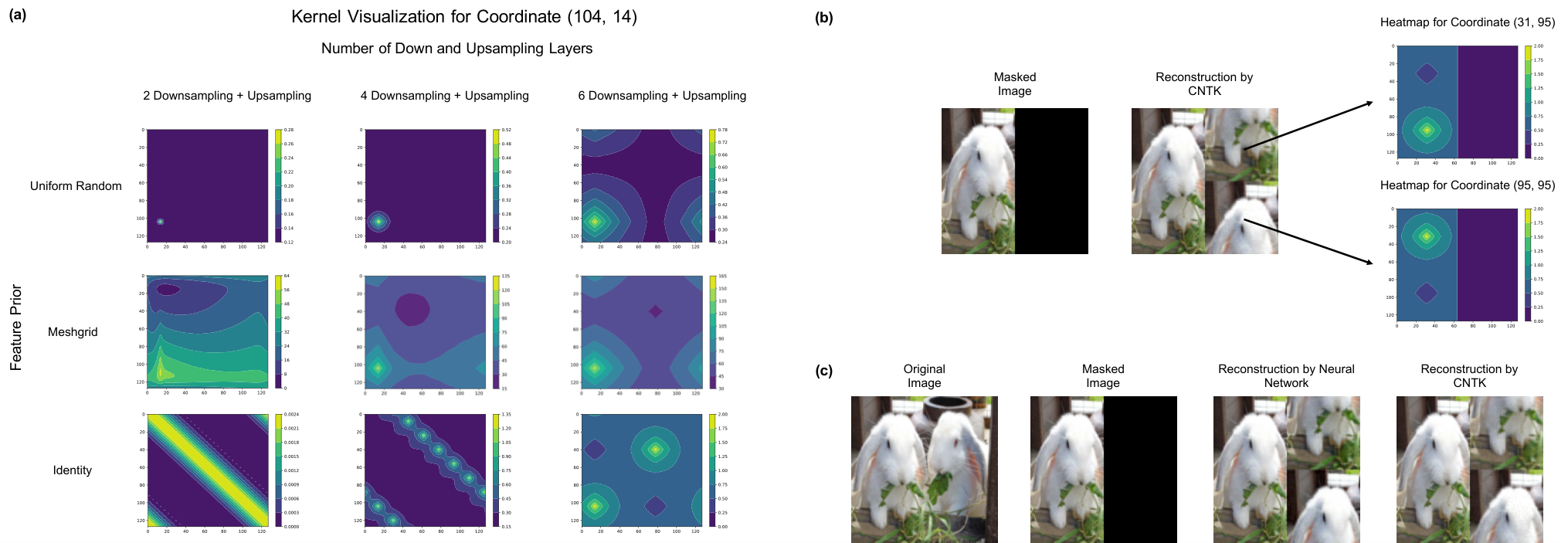
In Fig. 4a, we visualize the kernel values $K(104,14,:,:)$ computed for a $128\times 128$ image when varying the number of down and upsampling layers and as well as the feature prior $Z$ . Namely, we consider the cases where $Z$ is the identity, the meshgrid from [52], or the uniform random tensor used in large hole inpainting experiments of [52]. A key observation is that the kernel values for the uniform random feature prior are highest around the coordinate of interest regardless of the amount of down and upsampling, which is in stark contrast to other feature priors.³³ 3 When there are no downsampling and upsampling layers, this follows immediately from Theorem 2. This implies that neighboring pixels are most heavily used when imputing using the uniform random feature prior (see Appendix Fig. 11 for additional visualizations). Moreover, when using the uniform random feature prior, the amount of down and upsampling increase (by powers of 2) the size of the region considered for imputation (see the first row of Fig. 4a). These heatmaps identify the minimum amount of downsampling necessary for large hole inpainting: if there is an $m\times m$ region of missing pixels ( $m\geq 1$ ), we need at least $\lfloor\log_{2}(m+1)\rfloor$ layers of downsampling to ensure that no pixel is filled in as an average of all other pixels. This result explains the observation from [52], which showed that using neural networks with four or fewer downsampling and upsampling layers led to worse large hole inpainting performance on images with large missing regions.

The Identity Feature Prior is Ineffective for Image Completion

The standard feature prior for matrix completion is given by choosing $Z$ to be the identity matrix [3, 13, 22]. As shown in Fig. 4a, unlike the uniform random feature prior, the identity feature prior uses pixel observations from non-local regions for completion. Thus, we expect this feature prior to be ineffective for image completion tasks.

Fig. 4b shows the result of using the CNTK for a network with 6 downsampling and upsampling layers and the identity feature prior to impute a $128\times 128$ rabbit image. The identity feature prior visually appears to translate observed pixels from a non-local region to perform imputation. The regions that are being translated are precisely those given by the corresponding heatmaps, e.g. the upper right quadrant is imputed using the lower left quadrant in Fig. 4b.

We note that our framework accurately predicts the behavior of finite width neural networks used for image inpainting. In Fig. 4c, we show the result of using a neural network with 6 downsampling and upsampling layers, sigmoid activation on the last layer, and identity feature prior. We observe that the neural network completes the image by translating observed pixels similarly to the imputation provided by the corresponding CNTK. This example highlights the power of using our framework for rapidly prototyping feature priors and architectures for image inpainting tasks.

6 Discussion

In this work, we presented a simple, fast, and flexible framework for matrix completion using the infinite width limit of neural networks, i.e. the neural tangent kernel (NTK). Below, we highlight the aspects of our framework that enable such simplicity, speed, and flexibility.

•

Simple. Our framework is conceptually simple since we are using kernels to learn a map from features of coordinates, $(i,j)$ , to entries in the target matrix, $Y_{i,j}$ . Our framework is computationally simple since solving kernel regression involves solving a linear system of equations.
•

Fast. Our framework is naturally fast when using the NTK of fully connected networks for matrix completion due to the simple closed form of the kernel (Theorem 1). We develop a memory and runtime efficient algorithm to compute and use the NTK of convolutional networks (the CNTK) for matrix completion (Section 4).
•

Flexible. Our framework is easily adapted to various applications by the choice of the feature prior, thereby making our framework flexible. Moreover, we provided a principled approach for selecting the feature prior by establishing a connection with semi-supervised learning (Theorems 1, 2) and providing a visualization of the effect of the feature prior (Section 4).

The simplicity and speed of our framework is illustrated by the fact that many of our results (including inpainting high resolution images) can be run on a CPU and even on a laptop (see Materials & Methods for a link to our code). We demonstrated that our framework is flexible by using it to achieve competitive results for virtual drug screening (Section 3) and image inpainting/reconstruction (Section 5). We envision that our work provides a simple and accessible framework for producing strong baselines for several matrix completion applications. We conclude with a discussion of possible future extensions and applications.

Future Applications of Our Framework

In this work, we demonstrated the flexibility of our framework by constructing feature priors for two different applications, namely virtual drug screening and image completion. An interesting future direction is the extension of our framework to other modalities such as tensors, video, or audio data. For example, by using a feature prior that captures the structure of coordinates in 3D images, we could apply our framework to impute missing regions in three-dimensional data.

Efficient Computation of the CNTK

In classification and regression settings, a major hindrance for using the CNTK in practice is the computational complexity in computing the kernel for a large image dataset. In this work, we presented an expansion technique to efficiently compute and store the exact CNTK for inpainting high resolution images, which was previously considered infeasible [50, 15]. By understanding the properties of the CNTK that make it effective for image problems, we envision that similar techniques could be applied to produce efficient kernel machines for image classification.

Developing Techniques to Improve the Performance of the NTK

While a large number of techniques such as skip connections, batch normalization, etc. have been developed to augment the performance of neural networks, such techniques have yet to be adapted to improve the performance of kernels. The simplicity and effectiveness of the NTK and CNTK based on simple architectures considered in this work motivates the development of techniques to further boost the performance of the NTK and kernel methods in general.

Materials and Methods

For solving kernel regression with the NTK, we use the direct linear system solver from [39] when the number of equations is fewer than 30,000, and we use EigenPro [35, 34] otherwise. For training neural networks, we use the PyTorch library [40]. All methods requiring a GPU are run on a single NVIDIA Titan RTX GPU. Our experiments are run on a shared server with 4 Titan RTX GPUs, 128GB CPU RAM, and 64 threads.

For the virtual drug screening experiments, we use the subset of the CMap dataset [49] provided in [25]. A detailed description of all the methods (including random seeds and hyperparameters for DNPP and FaLRTC) and evaluation metrics for the virtual drug screening experiments is provided in Appendices C-H. A description of the t-test used for determining the significance of our results for virtual drug screening is presented in Appendix I. We provide code to replicate our results for the virtual drug screening experiments with the NTK, DNPP, FaLRTC, and mean over cell type in the footnote below⁴⁴ 4 https://github.com/uhlerlab/ntk_matrix_completion. We use the codebase from [25] for performing imputation with FaLRTC.

For the image completion applications, we use the datasets from [15, 52]. The rabbit image used in Fig. 4 is from [46] and is provided in our codebase (linked above). For the neural network and NTK methods used in our image inpainting and reconstruction experiments, we provide a description of all architectures and training hyperparameters in Appendix N.

We provide a library for computing and using the CNTK for image inpainting and reconstruction applications in the codebase linked above. Our library lets the user define a custom neural network (similarly to network definitions in PyTorch), and then provides a function to compute the CNTK from the given architecture. Our method for computing the CNTK runs entirely on the CPU, and we enable parallelization across CPU threads. Our library includes functions for computing the CNTK for networks with nearest neighbor and bilinear upsampling layers, which are not readily available in the Neural Tangents library [38]. We additionally provide functions to solve kernel regression using the CNTK via a linear system solver or EigenPro. A full description of the library and an example of how to use our library for image inpainting is provided in Jupyter notebooks in our linked code. We additionally release several pre-computed kernels that can be used for high resolution inpainting and reconstruction.

Acknowledgements

A.R., G.S., and C.U. were partially supported by NSF (DMS-1651995), ONR (N00014-17-1-2147 and N00014-18-1-2765), the MIT-IBM Watson AI Lab, the Eric and Wendy Schmidt Center at the Broad Institute, and a Simons Investigator Award (to C.U.). M.B. acknowledges support from NSF IIS-1815697 and NSF DMS-2031883/Simons Foundation Award 814639.

References

[1] Netflix prize rules, 2009. https://www.netflixprize.com/assets/rules.pdf.
[2] C. C. Aggarwal. Recommender Systems: The Textbook. Springer Publishing Company, Incorporated, 1st edition, 2016.
[3] S. Arora, N. Cohen, W. Hu, and Y. Luo. Implicit regularization in deep matrix factorization. In Advances in Neural Information Processing Systems, 2019.
[4] S. Arora, S. S. Du, W. Hu, Z. Li, R. Salakhutdinov, and R. Wang. On exact computation with an infinitely wide neural net. In Advances in Neural Information Processing Systems, 2019.
[5] P. L. Bartlett, P. M. Long, G. Lugosi, and A. Tsigler. Benign overfitting in linear regression. Proceedings of the National Academy of Sciences, 117(48):30063–30070, 2020.
[6] T. Becker, K. Yang, J. C. Caicedo, B. K. Wagner, V. Dancik, P. Clemons, S. Singh, and A. E. Carpenter. Predicting compound activity from phenotypic profiles and chemical structures. bioRxiv, https://doi.org/10.1101/2020.12.15.422887, 2020.
[7] M. Belkin, D. Hsu, S. Ma, and S. Mandal. Reconciling modern machine-learning practice and the classical bias–variance trade-off. Proceedings of the National Academy of Sciences, 116(32):15849–15854, 2019.
[8] M. Belkin, D. Hsu, and J. Xu. Two models of double descent for weak features. Society for Industrial and Applied Mathematics Journal on Mathematics of Data Science, 2(4):1167–1180, 2020.
[9] M. Belkin and P. Niyogi. Semi-supervised learning on riemannian manifolds. Machine Learning, 56:209–239, 2004.
[10] A. Belyaeva, L. Cammarata, A. Radhakrishnan, C. Squires, K. Yang, G. Shivashankar, and C. Uhler. Causal network models of SARS-CoV-2 expression and aging to identify candidates for drug repurposing. Nature Communications, 12(1024), 2021.
[11] A. Bietti and J. Mairal. On the inductive bias of neural tangent kernels. In Advances in Neural Information Processing Systems, 2019.
[12] R. Bouckaert and E. Frank. Evaluating the replicability of significance tests for comparing learning algorithms. In Pacific-Asia Conference on Knowledge Discovery and Data Mining, 2004.
[13] E. Candès and B. Recht. Exact matrix completion via convex optimization. Communications of the ACM, 55(6):111–119, 2012.
[14] E. J. Candès and T. Tao. The power of convex relaxation: Near-optimal matrix completion. Institute of Electrical and Electronics Engineers Transactions on Information Theory, 56(5):2053–2080, 2010.
[15] Z. Cheng, M. Gadelha, S. Maji, and D. Sheldon. A Bayesian perspective on the deep image prior. In Computer Vision and Pattern Recognition, 2019.
[16] Y. Cho and L. Saul. Kernel methods for deep learning. In Advances in Neural Information Processing Systems, 2009.
[17] S. B. Damelin and N. S. Hoang. On surface completion and image inpainting by biharmonic functions: Numerical aspects. International Journal of Mathematics and Mathematical Sciences, 2018.
[18] A. Daniely, R. F. Frostig, and Y. Singer. Toward deeper understanding of neural networks: The power of initialization and a dual view on expressivity. In Advances in Neural Information Processing Systems, 2016.
[19] A. Geifman, A. Yadav, Y. Kasten, M. Galun, D. Jacobs, and R. Basri. On the similarity between the laplace and neural tangent kernels. In Advances in Neural Information Processing Systems, 2020.
[20] R. Gonzalez and R. Woods. Digital Image Processing, volume 4. Pearson, 2018.
[21] I. Goodfellow, Y. Bengio, and A. Courville. Deep Learning, volume 1. MIT Press, 2016.
[22] S. Gunasekar, B. E. Woodworth, S. Bhojanapalli, B. Neyshabur, and N. Srebro. Implicit regularization in matrix factorization. In Advances in Neural Information Processing Systems, 2017.
[23] T. Hastie, A. Montanari, S. Rosset, and R. J. Tibshirani. Surprises in high-dimensional ridgeless least squares interpolation. arXiv:1903.08560, 2019.
[24] K. He, X. Zhang, S. Ren, and J. Sun. Deep residual learning for image recognition. In Computer Vision and Pattern Recognition, 2016.
[25] R. Hodos, P. Zhang, H.-C. Lee, Q. Duan, Z. Wang, N. R. Clark, A. Ma’ayan, F. Wang, B. Kidd, J. Hu, D. Sontag, and J. Dudley. Cell-specific prediction and application of drug-induced gene expression profiles. Pacific Symposium on Biocomputing, 23:32–43, 2018.
[26] M. Iwata, L. Yuan, Q. Zhao, Y. Tabei, F. Berenger, R. Sawada, S. Akiyoshi, M. Hamano, and Y. Yamanishi. Predicting drug-induced transcriptome responses of a wide range of human cell lines by a novel tensor-train decomposition algorithm. Bioinformatics, 35(14):191–199, 2019.
[27] A. Jacot, F. Gabriel, and C. Hongler. Neural Tangent Kernel: Convergence and generalization in neural networks. In Advances in Neural Information Processing Systems, 2018.
[28] J. Kaplan, S. McCandlish, T. Henighan, T. B. Brown, B. Chess, R. Child, S. Gray, A. Radford, J. Wu, and D. Amodei. Scaling laws for neural language models. arXiv:2001.08361, 2020.
[29] D. P. Kingma and J. Ba. Adam: A method for stochastic optimization. In International Conference on Learning Representations, 2015.
[30] O. Kwon, H. Lee, H.-J. Kong, E.-J. Kwon, J. Park, W. Lee, S. Kang, M. Kim, W. Kim, and H.-J. Cha. Connectivity map-based drug repositioning of bortezomib to reverse the metastatic effect of galnt14 in lung cancer. Oncogene, 39:1–14, 06 2020.
[31] J. Lee, S. S. Schoenholz, J. Pennington, B. Adlam, L. Xiao, R. Novak, and J. Shol-Dickstein. Finite versus infinite neural networks: an empirical study. In Neural Information Processing Systems, 2020.
[32] Z. Li, Z.-Q. J. Xu, T. Luo, and H. Wang. A regularized deep matrix factorized model of matrix completion for image restoration. arXiv:2007.14581, 2020.
[33] J. Liu, P. Musialski, P. Wonka, and J. Ye. Tensor completion for estimating missing values in visual data. Institute of Electrical and Electronics Engineers Transactions on Pattern Analysis and Machine Intelligence, 35(1):208–220, 2013.
[34] S. Ma and M. Belkin. Diving into the shallows: a computational perspective on large-scale shallow learning. In Advances in Neural Information Processing Systems, 2017.
[35] S. Ma and M. Belkin. Kernel machines that adapt to GPUs for effective large batch training. In Conference on Machine Learning and Systems, 2019.
[36] G. Meanti, L. Carratino, L. Rosasco, and A. Rudi. Kernel methods through the roof: handling billions of points efficiently. In Advances in Neural Information Processing Systems, 2020.
[37] P. Nakkiran, G. Kaplun, Y. Bansal, T. Yang, B. Barak, and I. Sutskever. Deep double descent: Where bigger models and more data hurt. In International Conference in Learning Representations, 2020.
[38] R. Novak, L. Xiao, J. Hron, J. Lee, A. A. Alemi, J. Sohl-Dickstein, and S. S. Schoenholz. Neural Tangents: Fast and easy infinite neural networks in Python. In International Conference on Learning Representations, 2020.
[39] T. E. Oliphant. A guide to NumPy, volume 1. Trelgol Publishing USA, 2006.
[40] A. Paszke, S. Gross, F. Massa, A. Lerer, J. Bradbury, G. Chanan, T. Killeen, Z. Lin, N. Gimelshein, L. Antiga, A. Desmaison, A. Kopf, E. Yang, Z. DeVito, M. Raison, A. Tejani, S. Chilamkurthy, B. Steiner, L. Fang, J. Bai, and S. Chintala. Pytorch: An imperative style, high-performance deep learning library. In Advances in Neural Information Processing Systems, 2019.
[41] T.-H. Phan, Y. Qui, J. Zeng, L. Xie, and P. Zhang. A deep learning framework for high-throughput mechanism-driven phenotype compound screening and its application to COVID-19 drug repurposing . Nature Machine Intelligence, 3:247–257, 2021.
[42] S. Pushpakom, F. Iorio, P. A. Eyers, K. J. Escott, S. Hopper, A. Wells, A. Doig, J. Guilliams, T. Latimer, C. McNamee, A. Norris, P. Sanseau, D. Cavalla, and M. Pirmohamed. Drug repurposing: progress, challenges and recommendations. Nature Reviews Drug Discovery, 18(1):41–58, 2019.
[43] A. Radhakrishnan, M. Belkin, and C. Uhler. Overparameterized neural networks implement associative memory. Proceedings of the National Academy of Sciences, 44(117):27162–27170, 2020.
[44] B. Recht, M. Fazel, and P. A. Parrilo. Guaranteed minimum-rank solutions of linear matrix equations via nuclear norm minimization. Society for Industrial and Applied Mathematics Review, 52(3):471–501, 2010.
[45] O. Ronneberger, P. Fischer, and T. Brox. U-Net: Convolutional networks for biomedical image segmentation. In International Conference on Medical Image Computing and Computer Assisted Intervention, 2015.
[46] O. Russakovsky, J. Deng, H. Su, J. Krause, S. Satheesh, S. Ma, Z. Huang, A. Karpathy, A. Khosla, M. Bernstein, A. C. Berg, and F.-F. Li. ImageNet large scale visual recognition challenge. International Journal of Computer Vision, 2015.
[47] B. Scholkopf and A. J. Smola. Learning with Kernels: Support Vector Machines, Regularization, Optimization, and Beyond. MIT Press, Cambridge, MA, USA, 2001.
[48] C. Squires, D. Shen, A. Agarwal, D. Shah, and C. Uhler. Causal imputation via synthetic interventions. arXiv:2011.03127, 2020.
[49] A. Subramanian, R. Narayan, S. M. Corsello, et al. A next generation connectivity map: L1000 platform and the first 1,000,000 profiles. Cell, 171(6):1437–1452, 2017.
[50] J. Tachella, J. Tang, and M. Davies. The neural tangent link between cnn denoisers and non-local filters. arXiv:2006.02379, 2020.
[51] R. Tsuchida, F. Roosta-Khorasani, and M. Gallagher. Invariance of weight distributions in rectified MLPs. In International Conference on Machine Learning, 2018.
[52] D. Ulyanov, A. Vedaldi, and V. Lempitsky. Deep Image Prior. In Conference on Computer Vision and Pattern Recognition, 2018.
[53] S. Van der Walt, J. L. Schönberger, J. Nunez-Iglesias, F. Boulogne, J. D. Warner, N. Yager, E. Gouillart, and T. Yu. scikit-image: image processing in Python. PeerJ, 2:e453, 2014.
[54] C. Williams and M. Seeger. Using the Nyström method to speed up kernel machines. In Advances in Neural Information Processing Systems, 2000.
[55] G. Williams, A. Gatt, E. Clarke, J. Corcoran, P. Doherty, D. Chambers, and C. Ballard. Drug repurposing for Alzheimer’s disease based on transcriptional profiling of human iPSC-derived cortical neurons. Translational Psychiatry, 9, 2019.
[56] B. Xu, N. Wang, T. Chen, and M. Li. Empirical evaluation of rectified activations in convolution network, 2015. arXiv:1505.00853.
[57] H. Xue, S. Zhang, and D. Cai. Depth image inpainting: Improving low rank matrix completion with low gradient regularization. Institute of Electrical and Electronics Engineers Transactions on Image Processing, 26:4311–4320, 2017.
[58] S. Zagoruyko and N. Komodakis. Wide residual networks. In Proceedings of the British Machine Vision Conference, 2016.
[59] C. Zhang, S. Bengio, M. Hardt, B. Recht, and O. Vinyals. Understanding deep learning requires rethinking generalization. In International Conference on Learning Representations, 2017.

Appendix

Appendix A Preliminaries on the NTK

In this section, we review notation from prior literature on the NTK [27] that will be used throughout this work. In particular, we review how the NTK can be computed in closed form using dual activation functions [18]. We start by providing the definition of the NTK.

Definition 2 (NTK).

Let $f(\mathbf{W};x):\mathbb{R}^{p}\times\mathbb{R}^{d}\to\mathbb{R}$ denote a neural network with parameters $\mathbf{W}$ . The neural tangent kernel, $K:\mathbb{R}^{d}\times\mathbb{R}^{d}\to\mathbb{R}$ , is a symmetric, continuous, positive definite function given by:

\displaystyle K(x,x^{\prime})=\langle\nabla_{\mathbf{W}}f(\mathbf{W}^{(0)};x),\nabla_{\mathbf{W}}f(\mathbf{W}^{(0)};x^{\prime})\rangle,

where $\mathbf{W}^{(0)}\in\mathbb{R}^{p}$ denotes the parameters at initialization.

In this section, we consider fully connected networks of the following form:

\displaystyle f(\mathbf{W};x)=W^{(L)}\frac{c}{\sqrt{k_{L}}}\phi\left(W^{(L-1)}\frac{c}{\sqrt{k_{L-1}}}\phi\left(\ldots\frac{c}{\sqrt{k_{1}}}\phi\left(W^{(1)}x\right)\ldots\right)\right),

(5)

where $\mathbf{W}=\{W^{(i)}\}_{i=1}^{L}$ with $W^{(i)}\in\mathbb{R}^{k_{i}\times k_{i-1}}$ and $k_{0}=d,k_{L}=1$ ; $\phi:\mathbb{R}\to\mathbb{R}$ is an elementwise Lipschitz nonlinearity; and $c$ is a constant. The key finding of [27] is that when $\mathbf{W}_{i}\overset{i.i.d.}{\sim}\mathcal{N}(0,1)$ , then as $k_{1},k_{2},\ldots k_{L}\to\infty$ , $K_{L}(x,x^{\prime})$ converges in probability to a deterministic kernel that does not change through training. Thus, solving kernel ridge-less regression with kernel $K_{L}$ is equivalent to the solution given by training the neural network. We present the case for fully connected networks from [27] below, but will also be using the results for convolutional networks from [4] later on.

Theorem.

Let $f:\mathbb{R}^{d}\to\mathbb{R}$ be a neural network defined in Eq. [5]. As $k_{1},k_{2},\ldots k_{L}\to\infty$ , then $K_{L}(x,x^{\prime})$ converges in probability to a deterministic kernel given by the following recurrences in $\Sigma_{i},\dot{\Sigma}_{i},K_{i}$ :

	$\displaystyle K_{0}(x,x^{\prime})$	$\displaystyle=\Sigma_{0}(x,x^{\prime})=x^{T}x^{\prime},$
	$\displaystyle K_{L}(x,x^{\prime})$	$\displaystyle=\Sigma_{L}(x,x^{\prime})+K_{L-1}(x,x^{\prime})\Sigma_{L-1}^{\prime}(\Sigma_{L-1}(x,x^{\prime})),$
	$\displaystyle\Sigma_{L}(x,x^{\prime})$	$\displaystyle=c^{2}\mathbb{E}_{(u,v)\sim\mathcal{N}(\mathbf{0},\Lambda_{L-1}(x,x^{\prime}))}[\phi(u)\phi(v)],$
	$\displaystyle\dot{\Sigma}_{L}(x,x^{\prime})$	$\displaystyle=c^{2}\mathbb{E}_{(u,v)\sim\mathcal{N}(\mathbf{0},\Lambda_{L-1}(x,x^{\prime}))}[\phi^{\prime}(u)\phi^{\prime}(v)],$
	$\displaystyle\Lambda_{L}(x,x^{\prime})$	$\displaystyle=\begin{bmatrix}\Sigma_{L-1}(x,x)&\Sigma_{L-1}(x,x^{\prime})\\ \Sigma_{L-1}(x^{\prime},x)&\Sigma_{L-1}(x^{\prime},x^{\prime})\end{bmatrix}.$

Dual Activations. The expectations in the recurrences above can be simplified using the theory of dual activation functions studied in [18]. Let $\check{\phi}:[-1,1]\to\mathbb{R}$ such that:

\displaystyle\check{\phi}(\xi)=c^{2}\mathbb{E}_{(u,v)\sim\mathcal{N}(\mathbf{0},\Lambda))}[\phi(u)\phi(v)],~~\Lambda=\begin{bmatrix}1&\xi\\ \xi&1\end{bmatrix},~~\frac{1}{\sqrt{2\pi}}\int_{\mathbb{R}}\phi(u)^{2}\exp{\left(-\frac{u^{2}}{2}\right)}du=\frac{1}{c^{2}}.

(6)

The map $\mathcal{F}$ such that $\mathcal{F}(\phi)=\check{\phi}$ is an operator mapping from activation functions to positive definite functions⁵⁵ 5 The map $\mathcal{F}$ is more precisely from the Hilbert space $L^{2}(\mu)$ with $\mu$ the Gaussian measure to the space of positive definite functions. The factor $c$ is selected so that $\|\phi\|_{L^{2}(\mu)}=1$ ., and $\check{\phi}$ is referred to as the dual activation [18]. The scaling factor $c$ in Theorem Theorem is typically selected to satisfy the integral equation in Eq. [6]. As an example, when $\phi$ is the ReLU, the integral is just $\frac{1}{2}$ times the second moment of the standard Gaussian distribution. Hence, $c=\sqrt{2}$ for the ReLU. The recurrence relation for the NTK can be drastically simplified for homogenous nonlinearities for which the dual activation has a closed form. As shown in prior work [16, 51], this is the case for the commonly used ReLU and LeakyReLU nonlinearities. In particular, the dual activation function for ReLU is well known [16], and we next present its form (with its derivative):

Lemma.

The dual activation $\hat{\phi}:[-1,1]\to\mathbb{R}$ of the ReLU is:

	$\displaystyle\check{\phi}(\xi)$	$\displaystyle=\frac{1}{\pi}(\xi(\pi-\cos^{-1}(\xi))+\sqrt{1-\xi^{2}})$		(7)
	$\displaystyle\frac{d\check{\phi}(\xi)}{d\xi}$	$\displaystyle=\frac{1}{\pi}(\pi-\cos^{-1}(\xi))$

As shown in [11, 19], the NTK recursion for ReLU networks can be simplified using the dual activation. We provide this known simplification below for completeness.

Proposition.

Let $f:\mathbb{R}^{d}\to\mathbb{R}$ be a neural network defined in Eq. 5. Let $\phi$ be the ReLU activation and let $c=\sqrt{2}$ . As $k_{1},k_{2},\ldots k_{L}\to\infty$ , then $K_{L}(x,x^{\prime})$ converges in probability to a deterministic kernel given by the following recurrences in $\Sigma_{i},K_{i}$ :

	$\displaystyle K_{0}(x,x^{\prime})$	$\displaystyle=\Sigma_{0}(x,x^{\prime})=x^{T}x^{\prime},$
	$\displaystyle\Sigma_{L}(x,x^{\prime})$	$\displaystyle=N_{L-1}(x,x^{\prime})\check{\phi}\left(\frac{\Sigma_{L-1}(x,x^{\prime})}{N_{L-1}(x,x^{\prime})}\right),$
	$\displaystyle K_{L}(x,x^{\prime})$	$\displaystyle=\Sigma_{L}(x,x^{\prime})+K_{L-1}(x,x^{\prime})\frac{d\check{\phi}}{d\xi}\left(\frac{\Sigma_{L-1}(x,x^{\prime})}{N_{L-1}(x,x^{\prime})}\right),$
	$\displaystyle N_{L-1}(x,x^{\prime})$	$\displaystyle=\sqrt{\Sigma_{L-1}(x,x)\Sigma_{L-1}(x^{\prime},x^{\prime})}.$

This proposition follows from using the change of variables $u=\sqrt{\Sigma_{L}(x,x)}\tilde{u}$ and $v=\sqrt{\Sigma_{L}(x^{\prime},x^{\prime})}\tilde{v}$ and the homogeneity of ReLU when computing $c^{2}\mathbb{E}_{(u,v)\sim\mathcal{N}(\mathbf{0},\Lambda_{L-1}(x,x^{\prime}))}[\phi(u)\phi(v)]$ using integration [11]. In this work, we will use the dual activation for both ReLU and LeakyReLU [56] in order to match popular deep learning architectures as closely as possible. The derivation for the dual activation for LeakyReLU is provided in [51].

Appendix B Proofs for Matrix Completion with the NTK

We present the statement of Theorem 1 for a general homogeneous (degree 1), Lipschitz nonlinearity below and then present the proof. We again note that ReLU and LeakyReLU are commonly used nonlinearities that satisfy these conditions. The results are easily extended to homogeneous nonlinearities of arbitrary degree and for feature priors that have columns with arbitrary norm.

Theorem.

Assume $Z=\{z^{(i)}\}_{i=1}^{n}\in\mathbb{R}^{p\times n}$ , where each column is normalized with $\|z^{(i)}\|_{2}=1$ . Let $f_{Z}(\mathbf{W})$ be a $d$ layer fully connected network with Lipschitz nonlinearity $\phi$ that is homogeneous of degree 1 and $c=\|\phi\|_{L^{2}(\mu)}^{-1}$ where $L^{2}(\mu)$ is the Hilbert space of square Lebesgue integrable functions under Gaussian measure. Then as layer widths $k_{1}\to\infty,k_{2}\to\infty,\ldots,k_{d-1}\to\infty$ , the NTK for matrix completion with $f_{Z}(\mathbf{W})$ is given by

\displaystyle K_{d}(M_{ij},M_{i^{\prime}j^{\prime}})=\begin{cases}\kappa_{d}({z^{(j)}}^{T}z^{(j^{\prime})})~~~\textrm{if }i=i^{\prime}\\ 0~~~~~~~~~~~~~~~~~~\textrm{if }i\neq i^{\prime}\end{cases},

where $\kappa_{d}(\xi)=\check{\phi}^{(d)}(\xi)+\kappa_{d-1}(\xi)\frac{d\check{\phi}}{d\xi}(\check{\phi}^{(d-1)}(\xi))$ , and $\check{\phi}^{(k)}(\xi)=\check{\phi}(\check{\phi}^{(k-1)}(\xi))$ for $k\geq 1$ and $\check{\phi}^{(0)}(\xi)=\xi$ .

Proof.

We proceed by induction and present the case for $d=1$ first. Namely, we define $g_{Z}(M)$ as follows:

\displaystyle g_{Z}(M)=tr(M^{T}A\phi(BZ)),

where $A\in\mathbb{R}^{m\times k},B\in\mathbb{R}^{k\times p},Z\in\mathbb{R}^{p\times n}$ . To compute the kernel, we compute $\frac{\partial g_{Z}(M)}{\partial A_{\alpha,\beta}},\frac{\partial g(M)}{\partial B_{\alpha,\beta}}$ directly. We begin by expanding the matrix products in $g_{Z}(M)$ . For a matrix $U$ , we let $U_{i,:}$ denote row $i$ of $U$ and $U_{:,i}$ denote column $i$ of $U$ . Note that

	$\displaystyle g_{Z}(M)$	$\displaystyle=tr\left(M^{T}A\frac{c}{\sqrt{k}}\phi(BZ)\right)$
		$\displaystyle=\frac{c}{\sqrt{k}}tr\left(M^{T}A\begin{bmatrix}\phi(B_{1,:}Z_{:,1})&\ldots&\phi(B_{1,:}Z_{:,n})\\ \vdots&\ldots&\vdots\\ \phi(B_{k,:}Z_{:,1})&\ldots&\phi(B_{k:}Z_{:,n})\end{bmatrix}\right)$
		$\displaystyle=\frac{c}{\sqrt{k}}tr\left(M^{T}\begin{bmatrix}\sum_{a=1}^{k}A_{1,a}\phi(B_{a,:}X_{:,1})&\ldots&\sum_{a=1}^{k}A_{1,a}\phi(B_{a,:}Z_{:,n})\\ \vdots&\ldots&\vdots\\ \sum_{a=1}^{k}A_{m,a}\phi(B_{a,:}X_{:,1})&\ldots&\sum_{a=1}^{k}A_{m,a}\phi(B_{a,:}Z_{:,n})\end{bmatrix}\right)$
		$\displaystyle=\frac{c}{\sqrt{k}}\sum_{i=1}^{m}\sum_{j=1}^{n}M_{i,j}\sum_{a=1}^{k}A_{i,a}\phi(B_{a,:}Z_{:,j}).$

We thus have that

	$\displaystyle\frac{\partial g_{Z}(M)}{\partial A_{\alpha,\beta}}$	$\displaystyle=\frac{c}{\sqrt{k}}\sum_{j=1}^{n}M_{\alpha,j}\phi(B_{\beta,:}Z_{:,j}),$
	$\displaystyle\frac{\partial g_{Z}(M)}{\partial B_{\alpha,\beta}}$	$\displaystyle=\frac{c}{\sqrt{k}}\sum_{i=1}^{m}\sum_{j=1}^{n}M_{i,j}A_{i,\alpha}\phi(B_{\alpha,:}Z_{:,j})Z_{\beta,j}.$

The NTK is given by:

	$\displaystyle K_{1}(M,\tilde{M})$	$\displaystyle=\langle\nabla g_{Z}(M),\nabla g_{Z}(M^{\prime})\rangle$
		$\displaystyle=\sum_{\alpha=1}^{m}\sum_{\beta=1}^{k}\frac{\partial g_{Z}(M)}{\partial A_{\alpha,\beta}}\cdot\frac{\partial g_{Z}(M^{\prime})}{\partial A_{\alpha,\beta}}+\sum_{\alpha=1}^{k}\sum_{\beta=1}^{p}\frac{\partial g_{Z}(M)}{\partial B_{\alpha,\beta}}\cdot\frac{\partial g_{Z}(M^{\prime})}{\partial B_{\alpha,\beta}}.$

To simplify the computation, we note that we will only ever need the gradient at indicator matrices $M_{ij}$ and $M_{i^{\prime}j^{\prime}}$ . Moreover, from the formula for the partial derivatives, we conclude that

	$\displaystyle\frac{\partial g_{Z}(M_{ij})}{\partial A_{\alpha,\beta}}$	$\displaystyle=\begin{cases}0&\text{if $\alpha\neq i$}\\ \frac{c}{\sqrt{k}}\phi(B_{\beta,:}Z_{:,j})&\text{otherwise}\end{cases},$
	$\displaystyle\frac{\partial g_{Z}(M_{ij})}{\partial B_{\alpha,\beta}}$	$\displaystyle=\frac{c}{\sqrt{k}}A_{i,\alpha}\phi(B_{\alpha,:}Z_{:,j})Z_{\beta,j}.$

Thus, we can simplify the NTK as follows:

	$\displaystyle\lim_{k\to\infty}K_{1}(M_{ij},M_{i^{\prime}j^{\prime}})$	$\displaystyle=\lim_{k\to\infty}\frac{c^{2}}{k}\sum_{\beta=1}^{k}\phi(B_{\beta,:}Z_{:,j})\phi(B_{\beta,:}Z_{:,j^{\prime}})\mathbf{1}_{i=i^{\prime}}$
		$\displaystyle~~~~~~~~~~+\frac{c^{2}}{k}\sum_{\alpha=1}^{k}A_{i,\alpha}A_{i^{\prime},\alpha}\sum_{\beta=1}^{p}\phi^{\prime}(B_{\beta,:}Z_{:,j})\phi^{\prime}(B_{\beta,:}Z_{:,j^{\prime}})Z_{\beta,j}Z_{\beta,j^{\prime}}$
		$\displaystyle=\begin{cases}0&i\neq i^{\prime}\\ \kappa_{1}({z^{(j)}}^{T}z^{(j^{\prime})})&i=i^{\prime}\end{cases},$

which completes the base case.

For the inductive step, we assume that

\displaystyle\lim_{k_{d-2}\to\infty}\ldots\lim_{k_{1}\to\infty}K_{d-1}(M_{ij},M_{i^{\prime}j^{\prime}})

\displaystyle=\begin{cases}0&i\neq i^{\prime}\\ \kappa_{d-1}({z^{(j)}}^{T}z^{(j^{\prime})})&i=i^{\prime}\end{cases}.

We now show that $K_{d}(M_{ij},M_{i^{\prime}j^{\prime}})$ has the desired form. For this, we define:

\displaystyle g_{Z}(M)=M^{T}A\frac{c}{\sqrt{k_{d-1}}}\phi(h_{Z}(\mathbf{W})),

where $A\in\mathbb{R}^{m\times k_{d-1}}$ and $h_{Z}(\mathbf{W}):\mathbb{R}^{p\times n}\to\mathbb{R}^{k_{d-1}\times n}$ is a $d-1$ fully connected network operating on $Z$ . Following the computation for the $1$ layer case, we obtain

	$\displaystyle\frac{\partial g_{Z}(M)}{\partial A_{\alpha,\beta}}$	$\displaystyle=\frac{c}{\sqrt{k_{d-1}}}\sum_{j=1}^{n}M_{\alpha,j}\phi(h_{Z}(\mathbf{W}))_{\beta,j},$
	$\displaystyle\frac{\partial g_{Z}(M)}{\partial\mathbf{W}_{\alpha,\beta}}$	$\displaystyle=\frac{c}{\sqrt{k_{d-1}}}\sum_{i=1}^{m}\sum_{j=1}^{n}M_{i,j}\sum_{k=1}^{k_{d-1}}A_{i,k}\frac{\partial{\phi(h_{Z}(\mathbf{W}))_{k,j}}}{\partial\mathbf{W}_{\alpha,\beta}}.$

Now we consider the case of indicator matrices $M_{ij},M_{i^{\prime}j^{\prime}}$ . For $M_{ij}$ , we note that $\frac{\partial g_{Z}(M)}{\partial A_{\alpha,\beta}}$ is only non-zero for the terms

\displaystyle\frac{\partial g_{Z}(M_{ij})}{\partial A_{i,\beta}}=\frac{c}{\sqrt{k_{d-1}}}\phi(h_{Z}(\mathbf{W}))_{\beta,j}.

Hence, if $i\neq i^{\prime}$ , we obtain that

\displaystyle\sum_{\alpha,\beta}\frac{\partial g_{Z}(M_{ij})}{\partial A_{\alpha,\beta}}\frac{\partial g_{Z}(M_{i^{\prime}j^{\prime}})}{\partial A_{\alpha,\beta}}=0.

Similarly, for $M_{ij}$ , we have that

\displaystyle\frac{\partial g_{Z}(M_{ij})}{\partial\mathbf{W}_{\alpha,\beta}}

\displaystyle=\frac{c}{\sqrt{k_{d-1}}}\sum_{k=1}^{k_{d-1}}A_{i,k}\frac{\partial{\phi(h_{Z}(\mathbf{W}))_{k,j}}}{\partial\mathbf{W}_{\alpha,\beta}}.

If $i\neq i^{\prime}$ , as $k_{d-1}\to\infty$ , by law of large numbers:

\displaystyle\sum_{\alpha,\beta}\frac{\partial g_{Z}(M_{ij})}{\partial B_{\alpha,\beta}}\frac{\partial g_{Z}(M_{i^{\prime}j^{\prime}})}{\partial B_{\alpha,\beta}}\to 0.

Thus, if $i\neq i^{\prime}$ , we conclude that $K_{d}(M_{ij},M_{i^{\prime}j^{\prime}})=0$ . On the other hand, if $i=i^{\prime}$ , then we have that

\displaystyle\sum_{\alpha,\beta}\frac{\partial g_{Z}(M_{ij})}{\partial A_{\alpha,\beta}}\frac{\partial g_{Z}(M_{i^{\prime}j^{\prime}})}{\partial A_{\alpha,\beta}}=\frac{c^{2}}{k_{d-1}}\sum_{k=1}^{k_{d-1}}\phi(h_{Z}(\mathbf{W}))_{k,j}\phi(h_{Z}(\mathbf{W}))_{k,j^{\prime}}.

(8)

Similarly, if $i=i^{\prime}$ , we have that

\displaystyle\sum_{\alpha,\beta}\frac{\partial g_{Z}(M_{ij})}{\partial B_{\alpha,\beta}}\frac{\partial g_{Z}(M_{i^{\prime}j^{\prime}})}{\partial B_{\alpha,\beta}}=\frac{c^{2}}{k_{d-1}}\left(\sum_{k=1}^{k_{d-1}}A_{i,k}\phi^{\prime}(h_{Z}(\mathbf{W}))_{k,j}\frac{\partial{h_{Z}(\mathbf{W})_{k,j}}}{\partial\mathbf{W}_{\alpha,\beta}}\right)\left(\sum_{k=1}^{k_{d-1}}A_{i,k}\phi^{\prime}(h_{Z}(\mathbf{W}))_{k,j^{\prime}}\frac{\partial{h_{Z}(\mathbf{W})_{k,j^{\prime}}}}{\partial\mathbf{W}_{\alpha,\beta}}\right)

By the inductive hypothesis as $k_{1},k_{2},\ldots k_{d-2}\to\infty$ , the above converges in probability to:

\displaystyle\lim_{k_{d-2}\to\infty}\ldots\lim_{k_{1}\to\infty}\sum_{\alpha,\beta}\frac{\partial g_{Z}(M_{ij})}{\partial B_{\alpha,\beta}}\frac{\partial g_{Z}(M_{i^{\prime}j^{\prime}})}{\partial B_{\alpha,\beta}}\to\frac{c^{2}}{k_{d-1}}\left(\sum_{k=1}^{k_{d-1}}\phi^{\prime}(h_{Z}(\mathbf{W}))_{k,j}\phi^{\prime}(h_{Z}(\mathbf{W}))_{k,j^{\prime}}K_{d-1}(M_{k,j},M_{k,j^{\prime}})\right).

(9)

Therefore, when $i=i^{\prime}$ , adding Eqs. [8] and [9] and applying the inductive hypothesis yields:

\displaystyle\lim_{k_{d-1}\to\infty}\lim_{k_{d-2}\to\infty}\ldots\lim_{k_{1}\to\infty}K_{d}(M_{ij},M_{i^{\prime}j^{\prime}})=\check{\phi}(\check{\phi}^{(d-1)}(\langle z^{(j)},z^{(j^{\prime})})\rangle)+K_{d-1}\frac{d\check{\phi}}{d\xi}\left(\check{\phi}^{(d-1)}(\langle z^{(j)},z^{(j^{\prime})}\rangle))\right),

which completes the proof. ∎

We next provide an example showing how to compute the NTK for matrix completion.

Example.

Suppose we have:

\displaystyle Y=\begin{bmatrix}y_{11}&.5&.3\\ .1&.2&y_{23}\\ .4&y_{32}&y_{33}\\ \end{bmatrix}.

Assuming we read off the observed entries of $Y$ in row major order and that $Z=I$ (the $3\times 3$ identity matrix), then the NTK is given by:

\displaystyle K=\begin{bmatrix}\kappa(1)&\kappa(0)&0&0&0\\ \kappa(0)&\kappa(1)&0&0&0\\ 0&0&\kappa(1)&\kappa(0)&0\\ 0&0&\kappa(0)&\kappa(1)&0\\ 0&0&0&0&\kappa(1)\end{bmatrix}.

The solution to kernel regression is given by:

\displaystyle\tilde{g}(M)=\begin{bmatrix}.5&.3&.1&.2&.4\end{bmatrix}K^{-1}k(M),

where $k(M)$ is the vector with entries $k(M_{ij},M)$ for $(i,j)\in S$ . As an example, for $M_{11}$ , we have:

\displaystyle k(M_{11})=\begin{bmatrix}\kappa(0)&\kappa(0)&0&0&0\end{bmatrix}^{T}.

This example demonstrates the key difference between the NTK of fully connected networks for matrix completion and the usual multivariate NTK: namely, the former corresponds to solving a separate kernel regression problem for each row of the target matrix $Y$ . By modifying the nonlinearity $\phi$ and the feature prior in Theorem 1, our framework encapsulates a broad class of semi-supervised learning approaches for matrix completion. We provide a nontrivial example below.

Example (Semi-supervised Learning with the Graph Laplacian).

The following corollary to Theorem 2 proves that semi-supervised learning using the graph Laplacian operator from [9] is a specific instance of matrix completion with the NTK of a linear neural network used for matrix completion.

Corollary.

Let $X\in\mathbb{R}^{d\times n}$ denote a set of data points of which a subset $X_{S}\in\mathbb{R}^{d\times s}$ is labelled with labels $Y_{S}\in\mathbb{R}^{1\times s}$ . Let $Z\in\mathbb{R}^{p\times n}$ denote the projection of $X$ onto the top $p$ eigenvectors of the graph Laplacian. Let $g_{Z}(M)=tr(M^{T}A\frac{1}{\sqrt{2k}}BZ)$ for $A\in\mathbb{R}^{1\times k},B\in\mathbb{R}^{k\times p}$ . Then as $k\to\infty$ , the following are equivalent:

\displaystyle\argmin_{A,B}\sum_{(i,j)\in S}(Y_{ij}-g_{Z}(M_{ij}))^{2}\Longleftrightarrow\argmin_{w\in\mathbb{R}^{p}}\|Y_{S}-wZ\|_{2}^{2}

in the sense that $g_{Z}(M_{ij})=wZ_{:,j}$ .

The proof follows immediately from Theorem 1 and the fact that the dual activation for $\phi(x)=x$ is $\check{\phi}(\xi)=\xi$ . The example above illustrates the generality of our framework for matrix completion. Moreover, semi-supervised learning with the graph Laplacian can naturally be extended by using the NTK for a nonlinear neural network instead of a linear neural network. Namely, instead of using the eigenvectors of the graph Laplacian, we can naturally extend the above corollary by using embeddings produced by autoencoders (Ch. 14 of [21]).

Note that the flexibility to learn a low-rank imputation or imputation with other structures via our framework is given by the feature prior, which incorporates the relationships between the coordinates of the target matrix. Indeed, varying the feature prior can drastically change the imputation given by the NTK, and the NTK with appropriate feature prior can even produce low-rank imputations, as shown by the following example below.

Example.

Consider the Netflix problem of movie rating imputation. Suppose the target matrix $Y$ is of the form

\displaystyle Y=\begin{bmatrix}1&2&y_{13}\\ 1&2&3\end{bmatrix},

where the rows of $Y$ represent users, the columns represent movies, and the coordinate $Y_{ij}$ represents the rating (from 1 to 5 stars) a user $i$ gave to movie $j$ . By first flattening the matrix $Y$ into $Y_{v}=[1,2,y_{13},1,2,3]$ , and then using our framework with feature prior,

\displaystyle Z=\begin{bmatrix}1&0&0&1&0&0\\ 0&1&0&0&1&0\\ 0&0&1&0&0&1\end{bmatrix},

leads to a low rank imputed matrix

\displaystyle\hat{Y}=\begin{bmatrix}1&2&3\\ 1&2&3\end{bmatrix}.

The above example is simplistic in that it produces a low rank imputation by assuming that the users are identical and using a one-hot embedding for the movies. In practice, one would use a feature prior that embeds users via external metadata (e.g. user age, gender, etc.) and our framework would predict similar ratings for users with similar metadata.

Appendix C Experimental Details for Virtual Drug Screening in CMAP

For this application, we consider the 978 genes $\times$ 2,130 drugs $\times$ 71 cell types “large” tensor from [25]. From this tensor, we extract the 15,855 non-null values, and leave out the cell types (‘SNU1040’, ‘HEK293T’, ‘HS27A’), as they have less than 10 drugs in the dataset (i.e. for these cell types, we would not be able to perform 10-fold cross validation). We exclude MCF7 from the dataset when using our method, since we use it to compute our feature prior, but we give all other methods training access to all MCF7 observations to ensure a fair comparison. This leaves us with a dataset of 14,336 samples, which are used for imputation. A link to download this dataset is given in [25], which we repeat here for convenience: https://github.com/clinicalml/dgc_predict.

For training DNPP and FaLRTC, we use the same hyper-parameters as in [25]. We implemented DNPP, mean over cell type, and our framework in Python in the above link. We use the Matlab code from [25] located via the following link: https://github.com/clinicalml/dgc_predict/FaLRTC.m. In order to make our results for FaLRTC accessible without Matlab, we provide the imputations from FaLRTC in the following folder: https://www.dropbox.com/sh/w23viwbm3py1dq1/AADQD3Bi_bLx4Z7X2hcLoUzXa?dl=0.

Appendix D Feature Prior for Drug Response Imputation

DNPP performs well for imputing the effect of drugs on cell types that have many observations in the training set, but performs poorly when imputing the effect of drugs on cell types with few observations in the training set. Thus, to improve on DNPP, we use a dual feature prior: one for imputing the effect of drugs on cell types with many (at least 150) observations in the training set (the dense regime), and another for imputing the effect of drugs on cell types with few (at most 150) observations in the training set (the sparse regime).

Since DNPP and FaLRTC both yield an imputation that captures similarity between cell type and drug combinations in the large observation regime, we can use the output of one of these methods as the feature prior for those cell types that had greater than 150 drugs in the training set. In particular, we chose the output of FaLRTC for the feature prior in the dense regime since applying our method with this feature prior yielded superior results. For all observed examples that were in the training set, we use the gene expression for the observation itself as the encoding. For all feature priors, we additionally concatenated a constant (1.5) times the identity matrix to ensure that the corresponding kernel is positive definite⁶⁶ 6 We chose the constant 1.5 by tuning this parameter to give highest Pearson r value on seed 512. We then used this constant for all other random seeds.. We then solved kernel regression exactly (using the numpy solve function [39]) for the NTK of a 1-hidden layer ReLU network.

For those cell types with few (less than 150 observations) in the training set, we used a feature prior that concatenates an embedding of the cell type and an embedding of the drug type. For the drug embedding, we used the gene expression of MCF7 treated with the same drug as the drug embedding, if available in the training set. If this vector was not available in the training set, we simply used the mean of all MCF7 observations. For the cell type embedding, we used the mean of all observations for the corresponding cell type available in the training set. We then normalized each cell embedding to have the same norm as the drug embedding to balance their contributions to dot products computed for the kernel. We re-scaled the embedding for the cell type by a factor of 1.25 to give the cell type additional weight over drug type⁷⁷ 7 This hyperparameter was selected to maximize Pearson r value for seed 512 and then fixed across all other random seeds.. Lastly, we normalized the concatenation of the embeddings and solved kernel regression via the closed form in Theorem 1. We refer to this feature prior as the MCF7 reference prior.

The code for computing our feature priors is available at https://github.com/uhlerlab/ntk_matrix_completion.

Appendix E One-hot Encoding for Drugs is Equivalent to Imputation with Mean Over Cell Type

The following result shows that using a feature prior consisting of a one-hot embedding for drugs leads to performing imputation using the mean over all observations for a given cell type.

Proposition 2.

Let $Y\in\mathbb{R}^{m\times n}$ denote the gene expression vectors for cell type $c$ with drugs $\{d_{j}\}_{j=1}^{n}$ , such that columns $\{y^{(j)}\}_{i=1}^{\ell}$ are observed and columns $\{y^{(j)}\}_{i=\ell+1}^{n}$ are missing. Let $A\in\mathbb{R}^{m\times k},B\in\mathbb{R}^{k\times p}$ , $\phi(x)=\max(x,0)$ , $g:\mathbb{R}^{m\times n}\to\mathbb{R}$ such that:

\displaystyle g(M)=tr\left(M^{T}A\frac{\sqrt{2}}{\sqrt{k\ell}}\phi(BZ)\right),

where $Z=I_{n\times n}$ (i.e. a one-hot encoding of the drug). Then for $i\in[m],j>\ell$ , the solution to kernel ridge-less regression with the NTK for $g$ is:

\displaystyle\tilde{g}(M_{ij})=\left(\frac{1}{2\pi-1}-\frac{\ell}{(2\pi-1)(2\pi-1+\pi\ell)}\right)\left(\frac{1}{\ell}\sum_{j=1}^{\ell}y_{i}^{(j)}\right).

Proof.

The proof relies on the fact that the kernel matrix $K$ for $g$ is a block diagonal matrix. In particular, as shown in the example in Section 3, there is one block, $K_{B_{i}}\in\mathbb{R}^{\ell\times\ell}$ , for each row of $Y$ (i.e. $m$ blocks), and $K_{B_{i}}$ has diagonal entries $\kappa(1)=2$ and off-diagonal entries $\kappa(0)=\frac{1}{\pi}$ . Hence, each block of the kernel matrix can be written as:

\displaystyle K_{B_{i}}=\frac{1}{\ell}\left(\left(2-\frac{1}{\pi}\right)I_{\ell\times\ell}+\frac{1}{\pi}J\right),

where $J\in\mathbb{R}^{\ell\times\ell}$ is the all ones matrix. By the Sherman-Morrison formula,

\displaystyle K_{B_{i}}^{-1}=\frac{1}{\ell}\left(\frac{\pi}{2\pi-1}I-\frac{\pi}{(2\pi-1)(2\pi-1+\pi\ell)}J\right),

and thus

\displaystyle\tilde{g}(M_{ij})=\begin{bmatrix}y_{i}^{(1)}&y_{i}^{(2)}&\ldots&y_{i}^{(\ell)}\end{bmatrix}K_{B_{i}}^{-1}\mathbf{1}\frac{1}{\pi\ell},

where $\mathbf{1}\in\mathbb{R}^{\ell}$ is the all ones vector. Hence,

\displaystyle\tilde{g}(M_{ij})=\left(\frac{1}{2\pi-1}-\frac{\ell}{(2\pi-1)(2\pi-1+\pi\ell)}\right)\left(\frac{1}{\ell}\sum_{j=1}^{\ell}y_{i}^{(j)}\right),

which completes the proof. ∎

Appendix F Feature Prior Corresponding to Previous Algorithms

As discussed in Section 2 of the main text, our framework provides a direct approach for improving upon previous methods for virtual drug screening. Using the output of DNPP and FaLRTC as the feature prior in our framework leads to an improvement; namely, across every round and fold in 5 rounds of 10-fold cross validation (using seeds $149,10,53,77,1928$ ), we find that our method with the DNPP output as a feature prior outperforms DNPP and that our method with the FaLRTC output as a feature prior outperforms FaLRTC. This is demonstrated in Figs. 5 and 6.

Appendix G Performance of Methods on Sparse versus Dense Subsets

We demonstrate in Fig. 7 that DNPP is effective for imputation on the dense regime (i.e. for those drug/cell type pairs with over 150 profiles), but not as effective in the sparse regime (i.e. for those drug/cell type pairs with less than 150 profiles). FaLRTC seems to perform comparably between the dense and the sparse regime, but under-performs DNPP on the full dataset.

Appendix H Metrics for Evaluation in Drug Response Imputation

Let $\hat{Y}\in\mathbb{R}^{m\times n}$ denote the concatenatation of the test predictions for all 10 folds and let $Y^{*}\in\mathbb{R}^{m\times n}$ denote the ground truth. We use ${y^{*}}^{(i)}$ to denote the $i^{th}$ column of $Y^{*}$ . Let $\bar{y}^{(i)}=c_{i}\mathbf{1}$ where $c_{i}=\sum_{j=1}^{m}y_{j}^{(i)}$ . For $A\in\mathbb{R}^{a\times b}$ , let $A_{v}\in\mathbb{R}^{a\cdot b}$ denote the vectorized version of $A$ . We use the following 3 metrics for evaluating the effectiveness of a given imputation method. All evaluation metrics have a maximum value of $1$ .

1. Pearson r value: This evaluation metric was used in [25] and is given by:

\displaystyle v=\frac{\langle\hat{Y}_{v},Y_{v}^{*}\rangle}{\|\hat{Y}_{v}\|_{2}\|Y_{v}^{*}\|_{2}}.

2.Mean $R^{2}$ : This evaluation metric is given by:

\displaystyle v=\frac{1}{n}\sum_{i=1}^{n}\left(1-\frac{\sum_{j=1}^{m}(\hat{y}_{j}^{(i)}-{y_{j}^{*}}^{(i)})^{2}}{\sum_{j=1}^{m}({y_{j}^{*}}^{(i)}-\bar{y}_{j}^{(i)})^{2}}\right).

3. Mean Cosine Similarity: This evaluation metric is given by:

\displaystyle v=\frac{1}{n}\sum_{i=1}^{n}\frac{\langle\hat{y}^{(i)},{y^{*}}^{(i)}\rangle}{\|\hat{y}^{(i)}\|_{2}\|{y^{*}}^{(i)}\|_{2}}.

Appendix I Statistical Significance of NTK on Drug Response Imputation

In experiments on the full dataset, we use 10-fold cross validation and 5 random seeds (149, 10, 77, 53, 1928) for comparing our method to DNPP from [25]. For each fold, we ensure that $10\%$ of the drugs for each cell type are present in the test set. To determine the statistical significance of our method for improving over DNPP, we use a one-sided test with the following corrected repeated k-fold cv test statistic for $r$ rounds of $k$ -fold cross validation (as described in Section 3.3 of [12]):

\displaystyle t=\frac{\frac{1}{kr}\sum_{i=1}^{k}\sum_{j=1}^{r}d_{ij}}{\left(\frac{1}{kr}+\frac{n_{2}}{n_{1}}\right)\hat{\sigma}^{2}},

where $d_{ij}$ is the difference between the evaluation metric for our method (the output of FaLRTC as the feature prior for the dense regime and the MCF7 reference feature prior for the sparse regime) and that of the DNPP for fold $k$ of round $j$ , $\hat{\sigma}$ is the estimated variance of the differences $d_{ij}$ , and $n_{1}$ is the number of samples used for training and $n_{2}$ is the number of samples used for testing (i.e. $\frac{n_{2}}{n1}\approx\frac{1}{9}$ for our setting). This statistic is distributed according to a t-distribution with $kr-1$ degrees of freedom. For the mean $R^{2}$ , we obtain $t=18.29$ and a corresponding p-value of $7.7\cdot 10^{-24}$ . For the mean cosine similarity, we obtain $t=14.75$ and a p-value of $5.9\cdot 10^{-20}$ . Thus, at a significance level of $.01$ , we reject the null hypothesis that our method and DNPP have the same performance.

Appendix J Matrix Completion with the CNTK

We repeat Proposition 1 from the main text and present the proof below. The tensor $\Theta\in\mathbb{R}^{m\times n\times m\times n}$ was defined and used in the computation of the CNTK for classification in [4].

Proposition.

Let $f_{Z}(\mathbf{W})$ be a $d$ layer convolutional network used to map from the feature prior $Z\in\mathbb{R}^{c\times r\times s}$ to the target matrix $Y\in\mathbb{R}^{m\times n}$ . Then as the number of convolutional filters per layer tends to infinity, the CNTK of $f_{Z}(\mathbf{W})$ is given by:

\displaystyle K(M_{ij},M_{i^{\prime}j^{\prime}})=[\Theta^{(d)}(Z,Z)]_{i,j,i^{\prime},j^{\prime}},

(10)

where $M_{ij},M_{i^{\prime}j^{\prime}}\in\mathbb{R}^{m\times n}$ denote indicator matrices.

Proof.

The proof follows almost immediately from the derivation of the CNTK for classification provided in [4]. Namely, let $g(M)=M^{T}f_{Z}(\mathbf{W})$ for $M\in\mathbb{R}^{m\times n}$ . Then, we have that:

\displaystyle\frac{\partial g(M)}{\partial\mathbf{W}_{\alpha,\beta}}=\sum_{i=1}^{m}\sum_{j=1}^{n}M_{i,j}\frac{\partial f_{Z}(\mathbf{W})_{i,j}}{\partial\mathbf{W}_{\alpha,\beta}}.

Thus, the kernel at the indicator matrices $M_{ij},M_{i^{\prime}j^{\prime}}$ is given by:

\displaystyle K(M_{ij},M_{i^{\prime}j^{\prime}})=\frac{\partial g(M_{ij})}{\partial\mathbf{W}_{\alpha,\beta}}\frac{\partial g(M_{i^{\prime}j^{\prime}})}{\partial\mathbf{W}_{\alpha,\beta}}=\frac{\partial f_{Z}(\mathbf{W})_{i,j}}{\partial\mathbf{W}_{\alpha,\beta}}\frac{\partial f_{Z}(\mathbf{W})_{i^{\prime},j^{\prime}}}{\partial\mathbf{W}_{\alpha,\beta}}=[\Theta(Z,Z)]_{i,j,i^{\prime},j^{\prime}},

which completes the proof. ∎

Below we additionally present an explicit derivation for the 1 hidden layer case for ReLU networks. This derivation will be useful in understanding the connection between the CNTK for matrix completion with semi-supervised learning from coordinate embeddings (i.e. Theorem 2 of the main text).

Proposition (1 Hidden Layer Convolutional Network).

Let $Z\in\mathbb{R}^{c\times m\times n}$ denote the feature prior. Let $*$ denote the neural network convolution operator and let $f_{Z}(\mathbf{W})=A*\frac{\sqrt{c}}{q\sqrt{k}}\phi(B*Z)$ denote a 1 hidden layer convolutional network where $B$ has $k$ filters of size $q\times q\times c$ with circular padding, $A$ has $1$ filter of size $q\times q\times k$ with circular padding for odd $q$ , $\phi$ is a homogeneous activation function of degree 1, and $c^{2}=\frac{1}{\mathbb{E}_{u\sim\mathcal{N}(0,1)}[\phi(u)^{2}]}$ . Let $K^{(0)},\tilde{K}^{(0)},\Sigma^{(0)}\in\mathbb{R}^{m\times n\times m\times n}$ such that:

\displaystyle\Sigma^{(0)}(i,j,i^{\prime},j^{\prime})=K^{(0)}(i,j,i^{\prime},j^{\prime})

\displaystyle=\sum_{\ell=1}^{c}\sum_{-\frac{q+1}{2}\leq m,n\leq\frac{q+1}{2}}Z_{\ell,i+m,j+n}Z_{\ell,i^{\prime}+m,j^{\prime}+n}.

If $M_{ij}$ and $M_{i^{\prime}j^{\prime}}$ are indicator matrices, then as $k\to\infty$ , the CNTK for $f_{Z}(\mathbf{W})$ is given by:

	$\displaystyle K(M_{ij},M_{i^{\prime}j^{\prime}})$	$\displaystyle=\frac{1}{q^{2}}\sum_{-\frac{q+1}{2}\leq a,b\leq\frac{q+1}{2}}\Sigma^{(1)}(i+a,j+b,i^{\prime}+a,j^{\prime}+b)$
		$\displaystyle~~~~~~~~~~+\dot{\Sigma}^{(1)}(i+a,j+b,i^{\prime}+a,j^{\prime}+b)K^{(0)}(i+a,j+b,i^{\prime}+a,j^{\prime}+b),$

where

	$\displaystyle\Sigma^{(1)}(i,j,i^{\prime},j^{\prime})$	$\displaystyle=\sqrt{\Sigma^{(0)}(i,j,i,j)\Sigma^{(0)}(i^{\prime},j^{\prime},i^{\prime},j^{\prime})}\hat{\phi}\left(\frac{\Sigma^{(0)}(i,j,i^{\prime},j^{\prime})}{\sqrt{\Sigma^{(0)}(i,j,i,j)\Sigma^{(0)}(i^{\prime},j^{\prime},i^{\prime},j^{\prime})}}\right),$
	$\displaystyle\dot{\Sigma}^{(1)}(i,j,i^{\prime},j^{\prime})$	$\displaystyle=\frac{d\hat{\phi}}{d\xi}\left(\frac{\Sigma^{(0)}(i,j,i^{\prime},j^{\prime})}{\sqrt{\Sigma^{(0)}(i,j,i,j)\Sigma^{(0)}(i^{\prime},j^{\prime},i^{\prime},j^{\prime})}}\right).$

Proof.

We provide the proof for the case of $1$ input channel ( $c=1$ ) below. The proof follows analogously for the case of multiple input channels. Let $g(M)=tr(M^{T}f_{Z}(\mathbf{W}))$ . Let $Y^{(\ell)}$ denote channel $\ell$ of $\frac{2}{\sqrt{k}}\phi(B*Z)$ and let $H=A*\frac{\sqrt{2}}{q\sqrt{k}}\phi(B*Z)$ . We thus have that

	$\displaystyle Y_{ij}^{(\ell)}$	$\displaystyle=\frac{\sqrt{c}}{q\sqrt{k}}\phi\left(\sum_{-\frac{q+1}{2}\leq a,b\leq\frac{q+1}{2}}Z_{i+a,j+b}B_{a,b}^{(\ell)}\right),$
	$\displaystyle H_{ij}$	$\displaystyle=\sum_{\ell=1}^{k}\sum_{-\frac{q+1}{2}\leq a,b\leq\frac{q+1}{2}}Y_{i+a,j+b}^{(\ell)}A_{a,b}^{(\ell)},$
	$\displaystyle g(M)$	$\displaystyle=\sum_{1\leq i,j\leq d}M_{ij}H_{ij}.$

Now we compute the partial derivatives of $f$ with respect to the parameters $A_{a,b}^{(\ell)}$ and $B_{m,n}^{(\ell)}$ :

	$\displaystyle\frac{\partial g(M_{ij})}{\partial A_{a,b}^{(\ell)}}$	$\displaystyle=Y_{i+a,j+b}^{(\ell)},$
	$\displaystyle\frac{\partial g(M_{ij})}{\partial B_{m,n}^{(\ell)}}$	$\displaystyle=\sum_{-\frac{q+1}{2}\leq a,b\leq\frac{q+1}{2}}A_{a,b}^{(\ell)}\frac{\sqrt{c}}{q\sqrt{k}}\phi^{\prime}\left(\sum_{-\frac{q+1}{2}\leq a^{\prime},b^{\prime}\leq\frac{q+1}{2}}Z_{i+a+a^{\prime},j+b+b^{\prime}}B_{a^{\prime},b^{\prime}}^{(\ell)}\right)Z_{i+a+m,j+b+n}.$

As $k\to\infty$ , the CNTK converges in probability to:

\displaystyle K(M_{ij},M_{i^{\prime}j^{\prime}})=\mathbb{E}_{A_{a,b}^{(\ell)},B_{m,n}^{(\ell)}\sim\mathcal{N}(0,1)}\left[\sum_{\ell=1}^{k}\sum_{a,b}\frac{\partial g(M_{ij})}{\partial A_{a,b}^{(\ell)}}\frac{\partial g(M_{i^{\prime}j^{\prime}})}{\partial A_{a,b}^{(\ell)}}+\sum_{\ell=1}^{k}\sum_{m,n}\frac{\partial g(M_{ij})}{\partial B_{m,n}^{(\ell)}}\frac{\partial g(M_{i^{\prime}j^{\prime}})}{\partial B_{m,n}^{(\ell)}}\right].

(11)

This expression can be simplified as follows:

	$\displaystyle K(M_{ij},M_{i^{\prime}j^{\prime}})$	$\displaystyle=\sum_{-\frac{q+1}{2}\leq a,b\leq\frac{q+1}{2}}\Sigma^{(1)}(i+a,j+b,i^{\prime}+a,j^{\prime}+b)$
		$\displaystyle~~~~~~~~~~+\dot{\Sigma}^{(1)}(i+a,j+b,i^{\prime}+a,j^{\prime}+b)K^{(0)}(i+a,j+b,i^{\prime}+a,j^{\prime}+b),$

where we have:

	$\displaystyle\Sigma^{(1)}$	$\displaystyle=\frac{c}{q^{2}}\mathbb{E}_{B_{a^{\prime},b^{\prime}}^{(\ell)}}\left[\sum_{a,b}\phi\left(\sum_{-\frac{q+1}{2}\leq a^{\prime},b^{\prime}\leq\frac{q+1}{2}}Z_{i+a+a^{\prime},j+b+b^{\prime}}B_{a^{\prime},b^{\prime}}^{(\ell)}\right)\phi\left(\sum_{-\frac{q+1}{2}\leq a^{\prime},b^{\prime}\leq\frac{q+1}{2}}Z_{i^{\prime}+a+a^{\prime},j^{\prime}+b+b^{\prime}}B_{a^{\prime},b^{\prime}}^{(\ell)}\right)\right]$
	$\displaystyle\dot{\Sigma}^{(1)}$	$\displaystyle=\frac{c}{q^{2}}\mathbb{E}_{B_{a^{\prime},b^{\prime}}^{(\ell)}}\left[\sum_{a,b}\phi^{\prime}\left(\sum_{-\frac{q+1}{2}\leq a^{\prime},b^{\prime}\leq\frac{q+1}{2}}Z_{i+a+a^{\prime},j+b+b^{\prime}}B_{a^{\prime},b^{\prime}}^{(\ell)}\right)\phi^{\prime}\left(\sum_{-\frac{q+1}{2}\leq a^{\prime},b^{\prime}\leq\frac{q+1}{2}}Z_{i^{\prime}+a+a^{\prime},j^{\prime}+b+b^{\prime}}B_{a^{\prime},b^{\prime}}^{(\ell)}\right)\right]$

Lastly, we reduce the above expressions by substituting in the values for $\Sigma^{(0)}$ from the statement of the proposition. Namely, let

	$\displaystyle u$	$\displaystyle=\sum_{a,b}\phi\left(\sum_{-\frac{q+1}{2}\leq a^{\prime},b^{\prime}\leq\frac{q+1}{2}}Z_{i+a+a^{\prime},j+b+b^{\prime}}B_{a^{\prime},b^{\prime}}^{(\ell)}\right),$
	$\displaystyle v$	$\displaystyle=\sum_{a,b}\phi\left(\sum_{-\frac{q+1}{2}\leq a^{\prime},b^{\prime}\leq\frac{q+1}{2}}Z_{i^{\prime}+a+a^{\prime},j^{\prime}+b+b^{\prime}}B_{a^{\prime},b^{\prime}}^{(\ell)}\right).$

Then, the above expressions for $\Sigma^{(1)},\dot{\Sigma^{(1)}}$ simplify to:

	$\displaystyle\Sigma^{(1)}$	$\displaystyle=\frac{c}{q^{2}}\mathbb{E}_{B_{a^{\prime},b^{\prime}}^{(\ell)}}\left[\phi(u)\phi(v)\right],$
	$\displaystyle\dot{\Sigma}^{(1)}$	$\displaystyle=\frac{c}{q^{2}}\mathbb{E}_{B_{a^{\prime},b^{\prime}}^{(\ell)}}\left[\phi^{\prime}(u)\phi^{\prime}(v)\right].$

Hence, we can use the formula for the dual activation of the ReLU to conclude that:

	$\displaystyle\Sigma^{(1)}(i,j,i^{\prime},j^{\prime})$	$\displaystyle=\frac{1}{q^{2}}\sqrt{\Sigma^{(0)}(i,j,i,j)\Sigma^{(0)}(i^{\prime},j^{\prime},i^{\prime},j^{\prime})}\check{\phi}\left(\frac{\Sigma^{(0)}(i,j,i^{\prime},j^{\prime})}{\sqrt{\Sigma^{(0)}(i,j,i,j)\Sigma^{(0)}(i^{\prime},j^{\prime},i^{\prime},j^{\prime})}}\right),$
	$\displaystyle\dot{\Sigma}^{(1)}(i,j,i^{\prime},j^{\prime})$	$\displaystyle=\frac{1}{q^{2}}\frac{d\check{\phi}}{d\xi}\left(\frac{\Sigma^{(0)}(i,j,i^{\prime},j^{\prime})}{\sqrt{\Sigma^{(0)}(i,j,i,j)\Sigma^{(0)}(i^{\prime},j^{\prime},i^{\prime},j^{\prime})}}\right).$

Lastly, we complete the proof by substituting these expressions for $\Sigma^{(1)},\dot{\Sigma}^{(1)}$ into the expression for $K(M_{ij},M_{i^{\prime}j^{\prime}})$ above. ∎

As implied by Proposition 1 above, the CNTK is a functional of pairs of coordinates of images, while the usual CNTK for classification operates on pairs of images [4]. To be more specific, consider the setting where the target matrix $Y$ is in $\mathbb{R}^{m\times n}$ . Then, the CNTK for matrix completion that we compute lies in $\mathbb{R}^{mn\times mn}$ . On the other hand, when given $n$ images for classification, the CNTK computed in [4] lies in $\mathbb{R}^{n\times n}$ and does not depend on the image size.

Appendix K Equivalence with Semi-Supervised Learning for the CNTK

In the following, we present the statement and proof of Theorem 2 from the main text with the precise form for $\tilde{\psi}$ .

Theorem.

Consider a convolutional network, $f_{Z}(\mathbf{W})$ , with $d$ hidden layers with homogeneous activation of degree 1 and in which all filters have size $q$ and circular padding. Let $Z\in\mathbb{R}^{c\times m\times n}$ satisfy:

\displaystyle\sum_{\ell=1}^{c}\sum_{-\alpha\leq a,b\leq\alpha}Z_{\ell,i+a,j+b}Z_{\ell,i^{\prime}+a,j^{\prime}+b}=\psi(|i-i^{\prime}|,|j-j^{\prime}|)

	$\displaystyle K_{d}(M_{ij},M_{i^{\prime}j^{\prime}})$	$\displaystyle=\tilde{\psi}(\|i-i^{\prime}\|,\|j-j^{\prime}\|)$
		$\displaystyle=\check{\phi}^{(d)}\left(\frac{\psi(\|i-i^{\prime}\|,\|j-j^{\prime}\|)}{\psi(0,0)}\right)\psi(0,0)+K_{d-1}(M_{ij},M_{i^{\prime}j^{\prime}})\frac{d\check{\phi}}{d\xi}\left(\check{\phi}^{(d-1)}\left(\frac{\psi(\|i-i^{\prime}\|,\|j-j^{\prime}\|)}{\psi(0,0)}\right)\right),$

where $\check{\phi}$ is the dual activation of $\phi$ , $\check{\phi}^{(d)}(\xi)=\check{\phi}(\check{\phi}^{(d-1)}(\xi))$ with $\check{\phi}^{(0)}(\xi)=\xi$ , and $K_{0}(M_{ij},M_{i^{\prime}j^{\prime}})=\psi(|i-i^{\prime}|,|j-j^{\prime}|)$ .

Proof.

We prove this by induction on the number of hidden layers $d$ . We begin with the base case for $d=1$ : The proof for this case follows from the proof of the Proposition for 1 hidden convolutional networks in Appendix J. Namely, we have:

	$\displaystyle K(M_{ij},M_{i^{\prime}j^{\prime}})$	$\displaystyle=\sum_{-\frac{q-1}{2}\leq a,b\leq\frac{q-1}{2}}\Sigma^{(1)}(i+a,j+b,i^{\prime}+a,j^{\prime}+b)$
		$\displaystyle~~~~~~~~~~+\dot{\Sigma}^{(1)}(i+a,j+b,i^{\prime}+a,j^{\prime}+b)K^{(0)}(i+a,j+b,i^{\prime}+a,j^{\prime}+b),$

where

	$\displaystyle\Sigma^{(1)}(i,j,i^{\prime},j^{\prime})$	$\displaystyle=\frac{1}{q^{2}}\sqrt{\Sigma^{(0)}(i,j,i,j)\Sigma^{(0)}(i^{\prime},j^{\prime},i^{\prime},j^{\prime})}\check{\phi}\left(\frac{\Sigma^{(0)}(i,j,i^{\prime},j^{\prime})}{\sqrt{\Sigma^{(0)}(i,j,i,j)\Sigma^{(0)}(i^{\prime},j^{\prime},i^{\prime},j^{\prime})}}\right),$
	$\displaystyle\dot{\Sigma}^{(1)}(i,j,i^{\prime},j^{\prime})$	$\displaystyle=\frac{1}{q^{2}}\frac{d\check{\phi}}{d\xi}\left(\frac{\Sigma^{(0)}(i,j,i^{\prime},j^{\prime})}{\sqrt{\Sigma^{(0)}(i,j,i,j)\Sigma^{(0)}(i^{\prime},j^{\prime},i^{\prime},j^{\prime})}}\right).$

Now since $\Sigma^{(0)}(i,j,i^{\prime},j^{\prime})=\psi(|i-i^{\prime}|,|j-j^{\prime}|)$ , we conclude that

	$\displaystyle\Sigma^{(1)}(i,j,i^{\prime},j^{\prime})$	$\displaystyle=\frac{1}{q^{2}}\psi(0,0)\check{\phi}\left(\frac{\psi(\|i-i^{\prime}\|,\|j-j^{\prime}\|)}{\psi(0,0)}\right),$
	$\displaystyle\dot{\Sigma}^{(1)}$	$\displaystyle=\frac{1}{q^{2}}\frac{d\check{\phi}}{d\xi}\left(\frac{\psi(\|i-i^{\prime}\|,\|j-j^{\prime}\|)}{\psi(0,0)}\right).$

Substituting the above into the expression for $K(M_{ij},M_{i^{\prime}j^{\prime}})$ , we obtain

	$\displaystyle K(M_{ij},M_{i^{\prime}j^{\prime}})$	$\displaystyle=\frac{1}{q^{2}}\sum_{-\frac{q+1}{2}\leq a,b\leq\frac{q+1}{2}}\psi(0,0)\check{\phi}\left(\frac{\psi(\|i-i^{\prime}\|,\|j-j^{\prime}\|)}{\psi(0,0)}\right)$
		$\displaystyle~~~~~~~~~~+\psi(\|i-i^{\prime}\|,\|j-j^{\prime}\|)\frac{d\check{\phi}}{d\xi}\left(\frac{\psi(\|i-i^{\prime}\|,\|j-j^{\prime}\|)}{\psi(0,0)}\right)$

Note that the summand no longer depends on $a,b$ , and thus we conclude that

\displaystyle K(M_{ij},M_{i^{\prime}j^{\prime}})=\psi(0,0)\check{\phi}\left(\frac{\psi(|i-i^{\prime}|,|j-j^{\prime}|)}{\psi(0,0)}\right)+\frac{d\check{\phi}}{d\xi}\left(\frac{\psi(|i-i^{\prime}|,|j-j^{\prime}|)}{\psi(0,0)}\right)\psi(|i-i^{\prime}|,|j-j^{\prime}|),

which completes the base case.

For the inductive step, we assume that the following holds for depth $d-1$ :

	$\displaystyle\Sigma^{(d-1)}(M_{ij},M_{i^{\prime}j^{\prime}})$	$\displaystyle=\frac{1}{q^{2}}\check{\phi}^{(d-1)}\left(\frac{\psi(\|i-i^{\prime}\|,\|j-j^{\prime}\|)}{\psi(0,0)}\right)\psi(0,0),$
	$\displaystyle\dot{\Sigma}^{(d-1)}(M_{ij},M_{i^{\prime}j^{\prime}})$	$\displaystyle=\frac{1}{q^{2}}\frac{d\check{\phi}}{d\xi}\left(\check{\phi}^{(d-2)}\left(\frac{\psi(\|i-i^{\prime}\|,\|j-j^{\prime}\|)}{\psi(0,0)}\right)\right),$
	$\displaystyle K_{d-1}(M_{ij},M_{i^{\prime}j^{\prime}})$	$\displaystyle=q^{2}\Sigma^{(d-1)}(M_{ij},M_{i^{\prime}j^{\prime}})+q^{2}K_{d-2}(M_{ij},M_{i^{\prime}j^{\prime}})\dot{\Sigma}^{(d-1)}(M_{ij},M_{i^{\prime}j^{\prime}}),$

and assume that $K_{d-1}(M_{ij},M_{i^{\prime}j^{\prime}})=K_{d-1}(M_{i+a,j+b},M_{i^{\prime}+a,j^{\prime}+b})$ for any $a,b\in\mathbb{Z}$ satisfying $i+a,i^{\prime}+a\in[m]$ and $j+b,j^{\prime}+b\in[n]$ (i.e. assume that $K_{d-1}$ is shift invariant). Now, let $S^{(d-1)}(M_{ij},M_{i^{\prime}j^{\prime}})$ be defined as follows:

\displaystyle S^{(d-1)}(M_{ij},M_{i^{\prime}j^{\prime}})=\sum_{-\frac{q-1}{2}\leq a,b,\leq\frac{q-1}{2}}\Sigma^{(d-1)}(M_{i+a,j+b},M_{i^{\prime}+a,j^{\prime}+b})=\check{\phi}^{(d-1)}\left(\frac{\psi(|i-i^{\prime}|,|j-j^{\prime}|)}{\psi(0,0)}\right)\psi(0,0).

Then, by the derivation of the CNTK in [4], we obtain

	$\displaystyle\Sigma^{(d)}(M_{ij},M_{i^{\prime}j^{\prime}})$	$\displaystyle=\frac{1}{q^{2}}\check{\phi}\left(\frac{S^{(d-1)}(M_{ij},M_{i^{\prime}j^{\prime}})}{\sqrt{S^{(d-1)}(M_{ij},M_{ij})S^{(d-1)}(M_{i^{\prime}j^{\prime}},M_{i^{\prime}j^{\prime}})}}\right)\sqrt{S^{(d-1)}(M_{ij},M_{ij})S^{(d-1)}(M_{i^{\prime}j^{\prime}},M_{i^{\prime}j^{\prime}})}$
		$\displaystyle=\frac{1}{q^{2}}\check{\phi}\left(\check{\phi}^{(d-1)}\left(\frac{\psi(\|i-i^{\prime}\|,\|j-j^{\prime}\|)}{\psi(0,0)}\right)\right)\psi(0,0),$

where the last equality follows from the fact that $\check{\phi}(1)=1$ . Following an analogous derivation for $\dot{\Sigma}^{(d-1)}$ , we obtain that

\displaystyle\dot{\Sigma}^{(d)}(M_{ij},M_{i^{\prime}j^{\prime}})

\displaystyle=\frac{1}{q^{2}}\frac{d\check{\phi}}{d\xi}\left(\check{\phi}^{(d-1)}\left(\frac{\psi(|i-i^{\prime}|,|j-j^{\prime}|)}{\psi(0,0)}\right)\right).

Hence, the CNTK $K_{d}(M_{ij},M_{i^{\prime}j^{\prime}})$ is given by:

	$\displaystyle K_{d}(M_{ij},M_{i^{\prime}j^{\prime}})$	$\displaystyle=\sum_{-\frac{q-1}{2}\leq a,b,\leq\frac{q-1}{2}}\Sigma^{(d)}(M_{i+a,j+b},M_{i^{\prime}+a,j^{\prime}+b})$
		$\displaystyle~~~~~~~~~~+K_{d-1}(M_{i+a,j+b},M_{i^{\prime}+a,j^{\prime}+b})\dot{\Sigma}^{(d)}(M_{i+a,j+b},M_{i^{\prime}+a,j^{\prime}+b})$
		$\displaystyle=q^{2}\Sigma^{(d)}(M_{ij},M_{i^{\prime}j^{\prime}})+q^{2}K_{d-1}(M_{ij},M_{i^{\prime}j^{\prime}})\dot{\Sigma}^{(d)}(M_{ij},M_{i^{\prime}j^{\prime}}),$

where the last line follows from the shift invariance of $K_{d-1}$ . Lastly, we have that $K_{d}$ is shift invariant since all of the terms $\Sigma^{(d)},\dot{\Sigma}^{(d)}$ and $K_{d-1}$ are shift invariant. Hence, the induction is complete and the theorem follows. ∎

Appendix L Derivation of the CNTK for Matrix Completion with Modern Architectures

Below, we derive the CNTK for networks with fixed linear transformations. We note a similar formula appears in the Appendix of [50], but does not appear to be derived for the cases of nearest neighbor upsampling, nearest neighbor downsampling, and bilinear upsampling.

Proposition.

Let $g(M)=tr(M^{T}Af_{Z}(\mathbf{W}))$ denote a neural network where $A\in\mathbb{R}^{mn\times pq}$ is a fixed (i.e. non-trainable) linear transformation and $f_{Z}(\mathbf{W})$ is a convolutional network under the NTK parameterization⁸⁸ 8 We assume $A$ operates on the vectorized version of $f_{Z}(\mathbf{W})$ and then the output is reshaped to size $m\times n$ before multiplication by $M^{T}$ .. Then the CNTK, $K\in\mathbb{R}^{mn\times mn}$ , for $g$ is given by:

\displaystyle K

\displaystyle=AK_{f}A^{T}\implies K(M_{ij},M_{i^{\prime}j^{\prime}})=\sum_{a=1}^{pq}\sum_{b=1}^{pq}A_{v(i,j),a}A_{v(i^{\prime},j^{\prime}),b}K_{f}(M_{v_{1}^{-1}(a),v_{2}^{-1}(a)},M_{v_{1}^{-1}(b),v_{2}^{-1}(b)}),

where $v:\mathbb{R}^{2}\to\mathbb{R}$ is the bijective map from a coordinate $(i,j)$ in a matrix $B$ to its position in the vectorized version of $B$ and $K_{f}\in\mathbb{R}^{pq\times pq}$ is the CNTK for $f$ .

Proof.

Let $w_{p}$ denote a weight in $f$ and let w denote the vector of all weights in $f$ . We thus have that

		$\displaystyle\frac{\partial g(M)}{\partial w_{p}}=\sum_{m,n}M_{m,n}\frac{\partial{[Af_{Z}(\mathbf{W})]_{v(m,n)}}}{\partial w_{p}}=\sum_{m,n}M_{m,n}\sum_{\ell=1}^{pq}A_{v(m,n),\ell}\frac{\partial{f_{Z}(\mathbf{W})_{\ell}}}{\partial w_{p}}$
		$\displaystyle\implies K(M_{ij},M_{i^{\prime}j^{\prime}})=\left\langle\sum_{a=1}^{pq}A_{v(i,j),a}\frac{\partial f_{Z}(\mathbf{W})_{a}}{\partial\textbf{w}},\sum_{b=1}^{pq}A_{v(i^{\prime},j^{\prime}),b}\frac{\partial f_{Z}(\mathbf{W})_{b}}{\partial\textbf{w}}\right\rangle=AK_{g}A^{T},$

which completes the proof. ∎

While the Proposition above generally implies that a a linear transformation requires evaluating a quadratic form when computing the CNTK, the matrix $A$ corresponding to layers used in practice is typically extremely sparse. Hence, the required computation is simplified drastically, as is demonstrated by the following corollaries (the proofs follow directly from the proposition above).

Corollary (Downsampling through Strided Convolution).

Let $\Sigma^{(\ell)},\dot{\Sigma}^{(\ell)},K^{(\ell)}\in\mathbb{R}^{d\times d\times d\times d}$ correspond to the tensors used in the CNTK for a depth $\ell$ convolutional network. Then, using downsampling with a stride of $2$ at step $\ell+1$ maps the tensors to $\Sigma^{(\ell+1)},\dot{\Sigma}^{(\ell+1)},K^{\ell+1}\in\mathbb{R}^{\frac{d}{2}\times\frac{d}{2}\times\frac{d}{2}\times\frac{d}{2}}$ as follows: $\forall~i,j,i^{\prime},j^{\prime}\equiv 0~(\hskip-5.69054pt\mod 2)$ ,

	$\displaystyle\Sigma^{(\ell+1)}\left(\frac{i}{2},\frac{j}{2},\frac{i^{\prime}}{2},\frac{j^{\prime}}{2}\right)$	$\displaystyle=\Sigma^{(\ell)}(i,j,i^{\prime},j^{\prime}),$
	$\displaystyle\dot{\Sigma}^{(\ell+1)}\left(\frac{i}{2},\frac{j}{2},\frac{i^{\prime}}{2},\frac{j^{\prime}}{2}\right)$	$\displaystyle=\dot{\Sigma}^{(\ell)}(i,j,i^{\prime},j^{\prime}),$
	$\displaystyle K^{(\ell+1)}\left(\frac{i}{2},\frac{j}{2},\frac{i^{\prime}}{2},\frac{j^{\prime}}{2}\right)$	$\displaystyle=K^{(\ell)}(i,j,i^{\prime},j^{\prime}).$

Corollary (Nearest Neighbor Upsampling).

Let $\Sigma^{(\ell)},\dot{\Sigma}^{(\ell)},K^{(\ell)}\in\mathbb{R}^{\frac{d}{2}\times\frac{d}{2}\times\frac{d}{2}\times\frac{d}{2}}$ correspond to the tensors used in the CNTK for a depth $\ell$ convolutional network. Then, using nearest neighbor upsampling with a scale factor of $2$ at step $\ell+1$ transforms the tensors to $\Sigma^{(\ell+1)},\dot{\Sigma}^{(\ell+1)},K^{(\ell+1)}\in\mathbb{R}^{d\times d\times d\times d}$ as follows:

	$\displaystyle\Sigma^{(\ell+1)}\left(i,j,i^{\prime},j^{\prime}\right)$	$\displaystyle=\Sigma^{(\ell)}\left(\left\lfloor\frac{i}{2}\right\rfloor,\left\lfloor\frac{j}{2}\right\rfloor,\left\lfloor\frac{i^{\prime}}{2}\right\rfloor,\left\lfloor\frac{j^{\prime}}{2}\right\rfloor\right),$
	$\displaystyle\dot{\Sigma}^{(\ell+1)}\left(i,j,i^{\prime},j^{\prime}\right)$	$\displaystyle=\dot{\Sigma}^{(\ell)}\left(\left\lfloor\frac{i}{2}\right\rfloor,\left\lfloor\frac{j}{2}\right\rfloor,\left\lfloor\frac{i^{\prime}}{2}\right\rfloor,\left\lfloor\frac{j^{\prime}}{2}\right\rfloor\right),$
	$\displaystyle K^{(\ell+1)}\left(i,j,i^{\prime},j^{\prime}\right)$	$\displaystyle=K^{(\ell)}\left(\left\lfloor\frac{i}{2}\right\rfloor,\left\lfloor\frac{j}{2}\right\rfloor,\left\lfloor\frac{i^{\prime}}{2}\right\rfloor,\left\lfloor\frac{j^{\prime}}{2}\right\rfloor\right).$

The computation for bilinear upsampling (Ch. 2.4 of [20]) is presented below. We primarily use the structure of the updates to $\Sigma,\dot{\Sigma},K$ to efficiently compute the CNTK when the channels of $X$ are drawn i.i.d. from a stationary distribution.

When bilinearly upsampling (Ch. 2.4 of [20]) an image $A\in\mathbb{R}^{d\times d}$ to an image $\tilde{A}\in\mathbb{R}^{2d\times 2d}$ , each coordinate of $\tilde{A}$ is a linear combination of four coordinates of $A$ . Namely for $\alpha=\frac{d-1}{2d-1}$ ,

\displaystyle\tilde{A}_{i,j}=\sum_{a,b\in\{0,1\}}\lambda^{(i,j)}_{a,b}A_{\lfloor\alpha i\rfloor+a,\lfloor\alpha j\rfloor+b},

and $\lambda_{a,b}^{i,j}$ is selected as follows. Let $r=\lfloor\alpha i\rfloor,c=\lfloor\alpha j\rfloor$ and let:

	$\displaystyle\ell_{r}$	$\displaystyle=\frac{r}{\alpha},u_{r}=\frac{r+1}{\alpha},\ell_{c}=\frac{c}{\alpha},u_{c}=\frac{c+1}{\alpha},$
	$\displaystyle X$	$\displaystyle=[u_{r}-r,r-\ell_{r}],Y=[u_{c}-c,c-\ell_{c}],C=\frac{1}{(u_{r}-\ell_{r})(u_{c}-\ell_{c})}.$

Then, $\lambda_{a,b}^{(i,j)}=CX_{a}Y_{b}$ for $a,b\in\{0,1\}$ . The CNTK tensors are now transformed as follows.

Corollary 1 (Bilinear Upsampling).

Let $\Sigma^{(\ell)},\dot{\Sigma}^{(\ell)},K^{(\ell)}\in\mathbb{R}^{\frac{d}{2}\times\frac{d}{2}\times\frac{d}{2}\times\frac{d}{2}}$ correspond to the tensors used in the CNTK for a depth $\ell$ convolutional network. Then, using bilinear upsampling with a scale factor of $2$ at step $\ell+1$ transforms the tensors to $\Sigma^{(\ell+1)},\dot{\Sigma}^{(\ell+1)},K^{\ell+1}\in\mathbb{R}^{d\times d\times d\times d}$ as follows:

	$\displaystyle\Sigma^{(\ell+1)}\left(i,j,i^{\prime},j^{\prime}\right)$	$\displaystyle=\sum_{a,b\in\{0,1\}}\sum_{a^{\prime},b^{\prime}\in\{0,1\}}\lambda_{a,b}^{(i,j)}\lambda_{a^{\prime},b^{\prime}}^{(i^{\prime},j^{\prime})}\Sigma^{(\ell)}\left(\lfloor\alpha i\rfloor+a,\lfloor\alpha j\rfloor+b,\lfloor\alpha i^{\prime}\rfloor+a^{\prime},\lfloor\alpha j^{\prime}\rfloor+b^{\prime}\right),$
	$\displaystyle\dot{\Sigma}^{(\ell+1)}\left(i,j,i^{\prime},j^{\prime}\right)$	$\displaystyle=\sum_{a,b\in\{0,1\}}\sum_{a^{\prime},b^{\prime}\in\{0,1\}}\lambda_{a,b}^{(i,j)}\lambda_{a^{\prime},b^{\prime}}^{(i^{\prime},j^{\prime})}\dot{\Sigma}^{(\ell)}\left(\lfloor\alpha i\rfloor+a,\lfloor\alpha j\rfloor+b,\lfloor\alpha i^{\prime}\rfloor+a^{\prime},\lfloor\alpha j^{\prime}\rfloor+b^{\prime}\right),$
	$\displaystyle K^{(\ell+1)}\left(i,j,i^{\prime},j^{\prime}\right)$	$\displaystyle=\sum_{a,b\in\{0,1\}}\sum_{a^{\prime},b^{\prime}\in\{0,1\}}\lambda_{a,b}^{(i,j)}\lambda_{a^{\prime},b^{\prime}}^{(i^{\prime},j^{\prime})}K^{(\ell)}\left(\lfloor\alpha i\rfloor+a,\lfloor\alpha j\rfloor+b,\lfloor\alpha i^{\prime}\rfloor+a^{\prime},\lfloor\alpha j^{\prime}\rfloor+b^{\prime}\right).$

Appendix M Efficient Computation of the CNTK for High Resolution Images

Computing and storing the CNTK exactly for high resolution images is computationally prohibitive when using a naive approach. In particular, [15] notes that the kernel $K$ for a $500\times 500$ ( $K\in\mathbb{R}^{500\times 500\times 500\times 500}$ ) resolution image requires roughly 233GB of memory, which is infeasible on common hardware. In order to overcome these computational limitations, [50] uses the Nyström method [54] to approximate the kernel. In this section, we will demonstrate that we can compute the exact CNTK in a memory and run-time efficient manner for any convolutional neural network with circular padding, strided convolution, and nearest neighbor upsampling layers by using a feature prior $Z$ that has infinitely many channels.

Our key insight is that once architecture is fixed, the the CNTK for low resolution images can be expanded to that for high resolution images. In particular, when the convolutional architecture can be applied to both images of resolution $d_{1}$ and $d_{2}$ with $d_{2}>d_{1}$ , we can expand the kernel for resolution $d_{1}$ , $K_{d_{1}}\in\mathbb{R}^{d_{1}\times d_{1}\times d_{1}\times d_{1}}$ , to a tensor of size $\mathbb{R}^{d_{1}\times d_{1}\times d_{2}\times d_{2}}$ , which can be indexed to match the entries of the kernel for resolution $d_{2}$ , $K_{d_{2}}\in\mathbb{R}^{d_{2}\times d_{2}\times d_{2}\times d_{2}}$ .

In order to expand the kernel for low resolution images to the one for high resolution images, we need only pad and permute the rows and columns of the low resolution matrix. We define the required operations formally below (using zero indexing for our matrices).

Definition 3 (Row and Column Rotation).

Let $\Pi_{i,j}:\mathbb{R}^{d\times d}\to\mathbb{R}^{d\times d}$ such that $\Pi_{i,j}(A)=P_{\pi_{i}}AP_{\pi_{j}}$ where $P_{\pi_{\ell}}$ is a permutation matrix with permutation $\pi_{\ell}(i)=(i+\ell)\hskip-2.84526pt\mod d$ .

Definition 4 (Minimum Padding).

Let $M:\mathbb{R}^{d_{1}\times d_{1}}\to\mathbb{R}^{d_{2}\times d_{2}}$ with $d_{2}\geq d_{1}$ such that $M(A)=\tilde{A}$ , where

\displaystyle\tilde{A}_{i,j}

\displaystyle=\begin{cases}A_{i,j}&i<d_{1},j<d_{1}\\ \min_{a,b\in[d_{1}]}A_{a,b}&\text{otherwise}\end{cases}.

Example.

The operator $\Pi_{i,j}$ rotates the rows of $A$ down by $i$ and rotates the columns of $A$ right by $j$ as follows:

\displaystyle A=\begin{bmatrix}A_{1,1}&A_{1,2}&A_{1,3}\\ A_{2,1}&A_{2,2}&A_{2,3}\\ A_{3,1}&A_{3,2}&A_{3,3}\end{bmatrix}\implies\Pi_{1,2}(A)=\begin{bmatrix}A_{3,2}&A_{3,3}&A_{3,1}\\ A_{1,2}&A_{1,3}&A_{1,1}\\ A_{2,2}&A_{2,3}&A_{2,1}\end{bmatrix}.

Minimum padding $M:\mathbb{R}^{2\times 2}\to\mathbb{R}^{4\times 4}$ expands a matrix as follows:

\displaystyle A=\begin{bmatrix}0.1&0.2\\ 0.3&0.4\\ \end{bmatrix}\implies M(A)=\begin{bmatrix}0.1&0.2&0.1&0.1\\ 0.3&0.4&0.1&0.1\\ 0.1&0.1&0.1&0.1\\ 0.1&0.1&0.1&0.1\end{bmatrix}.

The theorem below demonstrates how to construct the kernel for a high resolution image by expanding and indexing a low resolution kernel. We assume that all strided convolutional layers have a stride size of $2$ in each direction and all upsampling layers have a scaling factor of $2$ . For the following theorem, we also write the kernel $K\in\mathbb{R}^{mn\times mn}$ as a 4 dimensional tensor $K\in\mathbb{R}^{m\times n\times m\times n}$ , where $K(i,j,i^{\prime},j^{\prime}):=K(M_{ij},M_{i^{\prime}j^{\prime}})$ .

Theorem (CNTK Expansion).

Let $g$ denote a convolutional neural network with circular padding, $s$ downsampling with strided convolution layers and $s$ nearest neighbor upsampling layers used to inpaint images in $\mathbb{R}^{2^{s+1}\times 2^{s+1}}$ . Define the feature prior $Z^{(\ell)}=\{Z_{p}^{(\ell)}\}_{p=1}^{\infty}\subset\mathbb{R}^{2^{\ell}\times 2^{\ell}}$ for $\ell\in\mathbb{Z}_{+}$ such that:

\displaystyle\sum_{p=1}^{\infty}Z_{p,i,j}^{(\ell)}Z_{p,i^{\prime},j^{\prime}}^{(\ell)}=\begin{cases}C_{1}&i=i^{\prime}~,~j=j^{\prime}\\ C_{2}&\text{otherwise}\end{cases}.

(12)

Let $d_{2}=2^{p_{2}}$ such that $p_{2}>s+1$ . For $\alpha=2^{\beta}$ , let $K_{\alpha}$ denote the CNTK for $g$ when used to inpaint images in $\mathbb{R}^{\alpha\times\alpha}$ with feature prior $Z^{(\beta)}$ . Let $p=2^{s}$ , $i^{\prime}=i\hskip-2.84526pt\mod p,j^{\prime}=j\hskip-2.84526pt\mod p$ . Then for $i,j\in[d_{2}]$ , we compute $\tilde{K}\in\mathbb{R}^{p\times p\times d_{2}\times d_{2}}$ as follows:

\displaystyle\tilde{K}(i^{\prime},j^{\prime},:,:)=\Pi_{i^{\prime}-p,j^{\prime}-p}(M(\Pi_{p-i^{\prime},p-j^{\prime}}(K_{s+1}[i^{\prime},j^{\prime},:,:]))),

and we have:

\displaystyle K_{d_{2}}(i,j,:,:)=\Pi_{i-i^{\prime},j-j^{\prime}}\tilde{K}(i^{\prime},j^{\prime},:,:).

Proof.

To provide intuition for the general case, we first prove the result for $s=0$ . Using the Proposition from Appendix J and the conditions on $Z^{(\ell)}$ , we obtain

\displaystyle\Sigma^{(0)}(i,j,i^{\prime},j^{\prime})=K^{(0)}(i,j,i^{\prime},j^{\prime})=\begin{cases}q^{2}C_{1}~~\text{if $i=i^{\prime},j^{\prime}=j^{\prime}$}\\ q^{2}C_{2}~~\text{otherwise}\end{cases}.

Hence for any $\ell,\ell^{\prime}\geq 1$ with $\ell^{\prime}<\ell$ , we conclude that $K_{\ell}(i,j,i^{\prime},j^{\prime})=K_{\ell^{\prime}}(a,b,a^{\prime},b^{\prime})$ when $(i,j)\neq(i^{\prime},j^{\prime})$ and $(a,b)\neq(a^{\prime},b^{\prime})$ , and $K_{\ell}(i,j,i,j)=K_{\ell^{\prime}}(a,b,a,b)$ for all $i,j\in[2^{\ell}]$ and $a,b\in[2^{\ell^{\prime}}]$ . Hence, by permuting rows, columns and minimum padding $K_{\ell^{\prime}}$ , we can recover the kernel for $K_{\ell}$ . Note that for $\ell=0$ , we do not ever record a kernel entry for the case where $(i,j)\neq(i^{\prime},j^{\prime})$ and so minimum padding would pad with the incorrect minimum value of $K_{0}(0,0,0,0)$ . This is why we need to expand up from the kernel for images of dimension $2^{s+1}$ and not just from the kernel for images of dimension $2^{s}$ .

For $s>0$ , we rely on the nearest neighbor upsampling and downsampling corollaries from Appendix L to understand which entries of $K_{\ell}(i,j,i^{\prime},j^{\prime})$ are equal to $K_{\ell^{\prime}}(a,b,a^{\prime},b^{\prime})$ . Since $Z^{(\ell)},Z^{(\ell^{\prime})}$ have the same range $\{C_{1},C_{2}\}$ of channel-wise products, it suffices to identify the elements of $K_{\ell^{\prime}}$ that are equal. These elements will then naturally be equal in $K_{\ell}$ after minimum padding.

From [15], we have that down-sampling through strided convolution preserves stationarity, and so after $t$ downsampling and convolutional layers, we again have that $K_{\ell}^{(t)}(i,j,i^{\prime},j^{\prime})=K_{\ell^{\prime}}^{(t)}(a,b,a^{\prime},b^{\prime})$ when $(i,j)\neq(i^{\prime},j^{\prime})$ and $(a,b)\neq(a^{\prime},b^{\prime})$ , and $K_{\ell}^{(t)}(i,j,i,j)=K_{\ell^{\prime}}^{(t)}(a,b,a,b)$ for all $i,j\in[2^{\ell}]$ and $a,b\in[2^{\ell^{\prime}}]$ .

In general, upsampling (including nearest neighbor upsampling) does not preserve stationarity, as is discussed in [15]. However, nearest neighbor upsampling preserves equality (up to permutation) between $K_{\ell}(i,j,:,:)$ and $K_{\ell}(i^{\prime},j^{\prime},:,:)$ provided that $i\equiv i^{\prime}~(\hskip-5.69054pt\mod 2^{s})$ and $j\equiv j^{\prime}~(\hskip-5.69054pt\mod 2^{s})$ . This follows immediately from analyzing the output after nearest neighbor upsampling in the original image space. In the following, we provide an example.

Example.

Consider the output of nearest neighbor upsampling a single channel $Y\in\mathbb{R}^{2\times 2}$ to $\tilde{Y}\in\mathbb{R}^{4\times 4}$ :

\displaystyle Y=\begin{bmatrix}Y_{0,0}&Y_{0,1}\\ Y_{1,0}&Y_{1,1}\end{bmatrix}\implies\tilde{Y}=\begin{bmatrix}Y_{0,0}&Y_{0,0}&Y_{0,1}&Y_{0,1}\\ Y_{0,0}&Y_{0,0}&Y_{0,1}&Y_{0,1}\\ Y_{1,0}&Y_{1,0}&Y_{1,1}&Y_{1,1}\\ Y_{1,0}&Y_{1,0}&Y_{1,1}&Y_{1,1}\end{bmatrix}.

From the stationarity of $Z^{(\ell)}$ and since convolution and downsampling layers preserve stationarity, we have that the CNTK for the above output $K_{2}(i,j,:,:)$ equals (up to permutation) $K_{2}(i^{\prime},j^{\prime},:,:)$ whenever $i\equiv i^{\prime}~(\hskip-5.69054pt\mod 2)$ and $j\equiv j^{\prime}~(\hskip-5.69054pt\mod 2)$ since the corresponding entries in $\tilde{Y}$ have identical patterns of neighbors (i.e. a row or column permutation by $2^{s}$ does not affect the sums involved in the kernel computation).

Thus, we conclude that the range of entries in $K_{\ell^{\prime}}(a,b,:,:)$ and $K_{\ell}(i,j,:,:)$ are equal whenever both $i\equiv a~(\hskip-5.69054pt\mod 2^{s})$ and $b\equiv j~(\hskip-5.69054pt\mod 2^{s})$ . To complete the proof, we just permute and minimum pads the entries of $K_{\ell^{\prime}}(a,b,:,:)$ to align the expanded matrix such that entry $K_{\ell^{\prime}}(a,b,a,b)$ corresponds to $K_{\ell}(i,j,i,j)$ in the expanded matrix. ∎

Remarks. Note that the expansion trick provided in the theorem above solely depends on (1) the number of downsampling and nearest neighbor upsampling layers; (2) the feature prior $Z$ having special structure as described in (12); and (3) the convolutional layers using circular padding. It importantly does not depend on the number of layers, type of homogeneous activation function (i.e. ReLU or leakyReLU), or size of the convolutional filters used. Hence our expansion technique can be used on a range of architectures, as we also demonstrate in Section 4 of the main text. The permutations $\Pi_{p-i^{\prime},p-j^{\prime}},\Pi_{i^{\prime}-p,j^{\prime}-p}$ used to compute $\tilde{K}$ are essentially used to ensure that we perform minimum padding appropriately for kernel values at the kernel’s edges. Lastly, when there are $s$ downsampling and upsampling layers, the smallest image size we can expand from is an image of size $2^{s+1}\times 2^{s+1}$ . We cannot use images of size $2^{s}$ since the corresponding kernel will not contain the same minimum value as that for images of size $2^{s+1}$ .

Appendix N Experimental Details for Image Inpainting

In the following, we describe the hyperparameters used for training neural networks and solving kernel regression with the CNTK on the considered image inpainting and image reconstruction tasks.

N.1 Large Hole Inpainting

For all large hole inpainting experiments, we used the autoencoder architecture from [15] that has 6 downsampling and upsampling layers with no skip connections. On all images other than the “library” image, we trained using the Adam optimizer [29] for 1000 epochs with a learning rate $10^{-2}$ . For the “library” image, we trained using the Adam optimizer for 6000 epochs with a learning rate of $10^{-2}$ . We used a random seed of 15 for all libraries. For implementing Adam with Langevin dynamics, we used the code and data from [15] directly. We performed optimal early stopping for all neural networks, i.e. we chose the reconstruction that has the closest match in PSNR to the ground truth. While impossible to perform in practice, optimal early stopping allows us to compare the CNTK with the best possible result from the neural network.

For solving kernel regression with the CNTK, we trained using EigenPro [34, 35] for 10 epochs, i.e., we did not early stop for large hole inpainting tasks. We scaled all kernels by a factor of $0.5$ to ensure convergence with EigenPro.

N.2 Image Reconstruction

Below we list the architectures and training procedure for each image. For the neural networks, we always trained for 6000 epochs using Adam with a learning rate of $10^{-3}$ , which is the learning rate used in [52]. All neural networks have $128$ convolutional filters per layer as is the case in [52]. We trained the CNTK for the corresponding architecture with EigenPro for 50 epochs, unless otherwise specified. The architectures used nearest neighbor upsampling, unless otherwise specified. We observed that training longer or, ideally, direct solving kernel regression with the CNTK for networks with nearest neighbor upsampling led to the best PSNR results for image reconstruction tasks. This is consistent with [52] in which networks for image reconstruction are trained twice as long as those for large hole inpainting. A direct solve was only computationally feasible on $256\times 256$ resolution images.

•

“Barbara”: We use a network with 2 downsampling and upsampling layers.
•

“Boat”: We use a network with 6 downsampling and upsampling layers. We train the CNTK for 100 epochs.
•

“Camera Man”: We use a network with 6 downsampling and upsampling layers. We train the CNTK for 100 epochs.
•

“Couple”: We use a network with 6 downsampling and upsampling layers. We train the CNTK for 100 epochs.
•

“Finger”: We use a network with 3 downsampling and upsampling layers. We train the CNTK for 100 epochs.
•

“Hill”: We use a network with 6 downsampling and upsampling layers.
•

“House”: We use a network with 6 downsampling and upsampling layers. We solve kernel regression exactly using the numpy solve function.
•

“Lena”: We use a network with 6 downsampling and upsampling layers.
•

“Man”: We use a network with 6 downsampling and upsampling layers.
•

“Montage”: We use a network with 6 downsampling and upsampling layers. We solve kernel regression exactly using the numpy solve method.
•

“Peppers”: We use a network with 5 downsampling and upsampling layers with bilinear upsampling. We solve kernel regression exactly using the numpy solve method, but add diagonal regularization from [31]. In particular, for kernel $K\in\mathbb{R}^{p\times p}$ , we add $\frac{4\cdot 10^{-5}}{p}tr(K)I_{p\times p}$ to the kernel before using the numpy solve function.

Figure 5: Comparison between DNPP and using the output of DNPP as a feature prior. Using our method with the output of DNPP as a feature prior leads to an improvement in all metrics across every round of 10-fold cross validation in 5 seeds.

Figure 6: Comparison between FaLRTC and using the output of FaLRTC as a feature prior. Using our method with the output of FaLRTC as a feature prior leads to an improvement in all metrics across every round of 10-fold cross validation in 5 seeds.

Figure 7: Comparison between DNPP and FaLRTC in (a) the sparse regime (< 150 profiles per cell type) and (b) the dense regime (> 150 profiles per cell type). We observe that FaLRTC outperforms DNPP in almost every fold for all performance metrics in the sparse regime. On the other hand DNPP outperforms FaLRTC in the dense regime in every fold for all performance metrics. This result demonstrates that DNPP can be improved drastically in the sparse regime.

Figure 8: A comparison of PSNR, SSIM, and runtime for large hole image inpainting using our framework (CNTK), corresponding finite width neural networks, and biharmonic inpainting. We observe that the CNTK outperforms (in PSNR and SSIM) on average both biharmonic inpainting and finite neural networks with sigmoid last layer and batch normalization layers while maintaing a runtime that is comparable to these methods. The last column illustrates that using more advanced techniques such as Adam with Langevin dynamics [15] can be used to boost the performance of neural networks, but at additional computational cost.

Figure 10: A comparison of PSNR, SSIM, and runtime for image reconstruction using our framework (CNTK), corresponding finite width neural networks, and biharmonic inpainting. We observe that the CNTK performs (in PSNR and SSIM) on average comparably to biharmonic inpainting and outperforms corresponding finite neural networks with sigmoid last layer and batch normalization layers. While our method is slower than biharmonic inpainting, it is more flexible than this method (see Fig. 8), and it is in average much faster than training finite width neural networks for this application.