A Moving Embedded Boundary Approach For The Compressible Navier-Stokes Equations In A Block-Structured Adaptive Refinement Framework
Abstract
A computational technique has been developed to perform compressible flow simulations involving moving boundaries using an embedded boundary approach within the block-structured adaptive mesh refinement framework of AMReX. A conservative, unsplit, cut-cell approach is utilized and a ghost-cell approach is developed for computing the flux on the moving, embedded boundary faces. Various test cases are performed to validate the method, and compared with analytical, experimental, and other numerical results in literature. Inviscid and viscous test cases are performed that span a wide regime of flow speeds – acoustic (harmonically pulsating sphere), smooth flows (expansion fan created by a receding piston) and flows with shocks (shock-cylinder interaction, shock-wedge interaction, pitching NACA 0012 airfoil and shock-cone interaction). A closed system with moving boundaries – an oscillating piston in a cylinder, showed that the percentage error in mass within the system decreases with refinement, demonstrating the conservative nature of the moving boundary algorithm. Viscous test cases involve that of a horizontally moving cylinder at , an inline oscillating cylinder at , and a transversely oscillating cylinder at . The judicious use of adaptive mesh refinement with appropriate refinement criteria to capture the regions of interest leads to well-resolved flow features, and good quantitative comparison is observed with the results available in literature.
Keywords compressible flow, embedded boundary, moving bodies, cut-cell, adaptive refinement, AMReX
1 Introduction
Flows with moving boundaries are of high significance for a variety of applications in a wide range of flow regimes – low Reynolds number flows such as swimming fish [42, 17], moderate speed flows such as wind turbines [6], and high Mach number flows such as store separation from a tactical aircraft.
The term immersed boundary (IB) method encompasses all such methods that simulate viscous flows with immersed (or embedded) boundaries on grids that do not conform to the shape of these boundaries. A variety of numerical approaches have been used for computing the flow around moving bodies, and they can be broadly classified as – body-fitted mesh methods, and embedded boundary (EB) methods. Body-fitted mesh approaches such as the overset/Chimera approach [69] and the Arbitrary Lagrangian-Eulerian (ALE) approach [26, 38] require expensive regeneration of the mesh as the body moves, which becomes cumbersome with complex body motion [49, 64]. The embedded boundary method places the body within a Cartesian mesh which does not conform with the geometry, and hence does not require complex grid (re)generation. But such an approach requires sophisticated numerical schemes for computing the terms in the governing equations on and close to the moving body, and the imposition of boundary conditions at the embedded boundary.
The earliest work in immersed boundary methods is the diffuse interface approach by Peskin 1972, in which a two dimensional simulation of flow in a heart valve was performed. The boundary was replaced by a force field defined on the mesh points of the rectangular domain which was calculated from the configuration of the boundary. In order to link the representations of the boundary and fluid, since boundary points and mesh points need not coincide, a semi-discrete analog of the delta function was introduced. Later, Goldstein et al. 1993 used the idea to impose a force field along a surface and can vary in space and time, with a magnitude and direction opposing the local flow was applied to bring the flow to rest. Two dimensional flow around cylinders and three dimensional turbulent channel flow in riblet-covered surface were simulated. Later, a direct forcing approach was developed for rigid body problems, in which the forces at immersed boundaries were calculated based on the temporally discretized momentum equation [54, 29, 81, 71]. Another class of immersed boundary methods are the sharp-interface methods that have no smearing, and thus have an accurate representation of the geometry. The Ghost fluid Method (GFM) belongs to the class of sharp interface methods. Fedkiw et al. 1999 and Fedkiw 2002 developed the ghost fluid method for multiphase flows, in which the interface is tracked with a level set function, which gives the exact sub-cell interface location, and at the interface, an approximate Riemann problem is solved. Further improvements were made in the method by Liu et al. 2003 and Terashima and Tryggvason 2009. Tseng and Ferziger 2003 developed a ghost cell IB method for flows with complex geometries using a reconstruction procedure to determine the values in the ghost cells for enforcing the boundary conditions. Mittal et al. 2008 used the ghost-cell approach to develop a sharp interface method for incompressible flows with moving and deforming bodies. More recently, Brahmachary et al. 2018 developed a sharp interface method for high-speed, compressible, inviscid flows, which imposed the boundary conditions on the body geometry, and used a novel reconstruction procedure to compute the solution in the vicinity of the solid-fluid interface. Al-Marouf and Samtaney 2017 developed a multidimensional partial differential extrapolation approach to reconstruct the solution in the ghost fluid regions and imposing boundary conditions on the fluid-solid interface, coupled with a multi-dimensional algebraic interpolation for freshly cleared cells.
In contrast to the diffuse interface methods, cut-cell methods are piecewise linear "accurate" and are strictly conservative. One of the early studies of the cut-cell approach [23] computed the flow over single- and multi-element airfoils on two-dimensional Cartesian grids using a finite volume approach. Later, Pember et al. 1995 developed a Godunov method which used a volume-of-fluid approach for the fluid-body interface. Yang et al. 1997a developed a cut-cell method for static boundaries and later extended to moving boundaries [86, 87], in which the upwind fluxes on the interfaces of static cells were updated using an HLLC approximate Riemann solver and an exact Riemann solution for a moving piston is used to update moving solid boundaries. One of the earliest studies that employed adaptive mesh refinement in a cut-cell, Cartesian framework was by DeZeeuw and Powell 1993. They performed compressible flow simulations on single- and multi-element airfoils using Roe’s approximate Riemann solver and a solution-adaptive refinement to resolve the high gradient regions. The cut-cell approach was used by Hu et al. 2006 to solve multi-fluid and complex moving geometry problems for compressible flows in two dimensions. Other early studies that used the cut-cell approach involve simulations of viscous incompressible flows with complex boundaries [89], forced and natural convection problems in an incompressible framework [79] and computation of solid-liquid phase fronts [80]. There are a number of studies that used the approach for simulations of incompressible, two- and three-dimensional flows over complex geometries [4, 44, 62, 51]. Hartmann et al. 2009 developed a cut-cell approach using ghost cells which can be freely positioned in space, hence making the approach flexible in terms of the shape and size of the embedded boundaries. A linear least-squares method is used to reconstruct the cell center gradients in irregular regions of the mesh to compute the flux at the surface. Cheny and Botella 2010 developed a Cartesian grid/immersed boundary method for incompressible viscous flows in two-dimensions for moving complex geometries.
The use of explicit time discretization schemes in a cut-cell approach leads to the classical small-cell issue. The Courant-Friedrichs-Lewy (CFL) restriction is based on the fluid volume in a cell, and hence will cause the admissible time step to be extremely small for cells with low volume fractions. Noh 1963 did some of the earliest work on this using a cell-merging and redistribution technique. The cell-merging technique identifies a cluster of cells around a cut-cell and merges them to form a larger control volume, and computes the flux update for this newly formed, merged control volume. The cell-merging technique was used by Bayyuk et al. 1993 for moving and deforming bodies, and by Quirk 1994 in a block-structured adaptive framework. This technique has been used for compressible flows with moving complex geometries [87], and compressible, multi-solid/fluid systems [7]. Though widely used, Schneiders et al. 2013 showed that the technique can lead to unphysical oscillations for moving boundary problems, and developed a method that used a smooth discrete formulation when cells are freshly cleared or covered by the moving boundary. Kirkpatrick et al. 2003 developed a novel cell-linking algorithm, which avoids the complexities involved with the cell-merging approach. Another technique to address the small-cell issue is the -box method [11, 48, 15], which approximates the numerical fluxes at the interfaces of a small cell based on initial values specified over regions of length - size of a regular grid cell, which will allow for the time step to be based on the regular grid size, rather than the small cell. In the current work, we use the flux redistribution technique [60, 24]. This involves updating the cut-cells using a hybrid divergence – a linear combination of the flux divergence of the cut-cell and the non-conservative divergence computed using the neighboring cell divergences, and then redistributing the “excess" quantity of the conserved variables to a neighborhood region of the cut-cell to ensure global conservation. Ji et al. 2010 used a cut-cell approach for detonation simulations with a cell-merging technique to avoid the small-cell issue. Muralidharan and Menon 2016 developed a novel cell clustering approach to treat the small-cell issue and maintain stability. The central idea was to employ a -order, polynomial piecewise approximation of the flow solution to a cluster of cells, and also extended it for moving boundary problems [58]. More recently, Sharan et al. 2020 have developed a method for deriving higher-order, provably stable schemes that avoids the small cell issue in a finite difference, cut-cell framework.
Immersed boundary methods offer a significant advantage in the simulation of flows with moving boundaries, and there have been a number of studies in this context [33, 88, 43, 52]. But the cut-cell approach presents additional challenges when applied to moving boundary problems. In particular, cut-cell based approach to high-speed, moving body problems require special care, and hence, the number of studies is limited. One of the earliest studies was by Yang et al. 1997b, Yang et al. 2000, in which the finite volume, unsplit MUSCL–Hancock method of the Godunov type was modified for moving boundaries, in conjunction with a cell-merging technique to maintain numerical stability in the presence of arbitrarily small cut cells to ensure strict conservation at the moving boundaries. Schneiders et al. 2013 showed that the widely used cell-merging technique creates unphysical oscillations for moving boundary problems, and developed an accurate moving boundary formulation based on the varying discretization operators which avoids the oscillations. Muralidharan and Menon 2018 developed a second-order cut-cell approach for flows with moving boundaries enforcing strict conservation using the small-cell clustering algorithm [57]. The cell clustering algorithm also preserves the smoothness of solution near moving surfaces. Bennett et al. 2018 employed a directional operator splitting method by extending the cut-cell approach for static walls from Klein et al. 2009. The scheme calculates the fluxes needed for a conservative update of the near-wall cut-cells as linear combinations of fluxes, which were obtained without regard to the small sub-cell problem, from a one-dimensional extended stencil. Tan and Shu 2011 developed a high order numerical boundary condition for compressible inviscid flows involving complex moving geometries. Their methodology was based on finite difference methods which was an extension of the inverse Lax–Wendroff procedure [72] for conservation laws in static geometries.
Fluid flow simulations with predictive capability require high resolution and superior parallel performance of the flow solvers, and this inevitably leads to the need for adaptive mesh refinement (AMR) strategies. In particular, for moving body problems, where the flow features that are of interest constantly change with time, solution-adaptive refinement can result in a significant reduction in compute time and memory. However, issues of deciding when and how to adapt, and keeping track of the evolving mesh, have to be addressed carefully for scalable performance. The cell-based tree data structure, which is very widely used for AMR, is very flexible, and provides a systematic way to keep track of the mesh. However, since each node of a cell-based tree is a single cell, computations suffer from significant overhead due to indirect addressing and lower FLOP rates are achieved [70]. Similar performance issues arise with general unstructured grids as well. Block-structured adaptive mesh refinement (SAMR) is more advantageous in many respects compared to the cell-based tree and unstructured grids [70]. Loop and cache optimizations can be performed over the arrays of cells when using adaptive blocks. The cost of neighbor pointers are amortized over entire arrays, and their ghost cell to computational cell ratio is superior to other data structures. Since the blocks permit refinement of larger multi-cell regions at a time, mesh adaptation is required less frequently than other data structures, which reduce computational cost. A number of frameworks exist for SAMR – BoxLib, Cactus, Chombo, Enzo, FLASH, and Uintah, are some of the publicly available frameworks. A survey of these frameworks can be found in Dubey et al. 2014.
In the current work, we use AMReX [1, 90] – a publicly available software framework for building massively parallel SAMR applications with C++ and Fortran interfaces. The features include parallelization via flat MPI, OpenMP, hybrid MPI/OpenMP, or MPI/MPI, GPUs, logical tiling of grids, support for multilevel mesh operations such as coarsening/interpolation between different levels and ghost cell filling, multigrid solvers for Poisson and Helmholtz equations, sub-cycling time-stepping algorithm, and support for particles and particle-mesh operations. The block-structured adaptive refinement strategy is based on the work of Berger 1982, and has been subsequently employed in various studies [13, 14, 9, 12, 19].
In this paper we devise a strategy for moving boundary problems for the compressible, Navier-Stokes equations within the finite-volume, block-structured adaptive mesh refinement framework of AMReX. The paper is organized as follows. Section 2 describes the algorithm for the cut-cell approach with static boundaries and its extension to moving boundaries. The numerical results for one-, two-, and three-dimensional compressible flow problems and comparison with experiments and other cases in literature are demonstrated in Section 3. Conclusion are given in Section 4.
2 The flow solver
The flow solver employs a finite volume, second order method to solve the compressible Navier-Stokes equations, given by
where ) is the vector of intensive conserved quantities – density, momentum and total energy, averaged over the cell with volume , is the flux vector (including both inviscid and viscous fluxes), denotes the surface of the finite volume region, is the outward normal to the surface and denotes the source terms. A Godunov approach is used to discretize the advection terms and Riemann solver evaluates the single-valued conservative fluxes on each cell face based on Van Leer-limited solution gradients of the transformed characteristic variables. The temporal discretization uses the second-order Runge-Kutta method. The flow solver [2] is implemented within the block-structured adaptive mesh refinement (AMR) framework of AMReX [90]. An embedded boundary (EB) approach is used to modify the finite volume discretization near complex geometries [24, 53]. The EB approach uses the volume fraction of the cut-cells, the area fraction of the cut-cell faces, the face normals, and the fluid volumetric centroid for the flux computation. In a naive formulation of the embedded boundary approach, the update in a cut-cell is given by (the source terms are omitted)
where is the volume fraction of the cut-cell. If we use an explicit time advancement scheme, then this leads to the classical small cut-cell issue. As , the CFL restriction results in the admissible time step . The technique of flux redistribution is utilized to treat the issue [24, 60], and is described here for completeness. This involves a two-step procedure – a hybrid divergence update of the cut-cells, and a redistribution of “excess” in the conserved quantity to the neighboring cells. The hybrid divergence is a volume fraction weighted average of the conservative () and non-conservative divergences (), and the update with the hybrid divergence is given by
The conservative divergence is given by the standard finite-volume expression
and hence the update can be written as
thereby avoiding the volume fraction appear explicitly in the denominator. Note that this approach circumvents the CFL restriction that leads to vanishing small time steps for small , however it is not strictly conservative. The non-conservative divergence contribution is computed as a weighted average of the conservative divergences of the neighboring cells as
where is the set of all reachable cells containing fluid in a 333 cell neighborhood. A flux redistribution technique following that described in Colella et al. 2006 is used to modify this update and ensure conservation. Had we only used the conservative divergence for the cut-cell , a conservative update would be
The hybrid update instead is
The latter expression leads to excess “mass” (mass refers to any of the conserved variables) in the EB cell given by
This excess mass is subtracted from the neighbors of the cut-cell. Let , and the total mass to be redistributed is
| (1) |
where is the set of neighboring cells and is the portion of redistributed mass that is to be added to the neighbor. Now, let us assign weights to the cells, which will determine the amount of redistributed quantity it gets. A cell with weight gets a volume averaged redistributed quantity , and Eq. 1 implies . There are a number of choices for how to partition the redistribution. If, for example, the redistribution is volume-weighted (assuming equal volumes for all cells), and
note that . Other strategies include upwind and/or mass weighting the distribution. For simplicity here, we select the volume-weighting scheme,
Hence, the final update for every cell in the domain (fluid cells and cut-cells) is given by
where is the update obtained using the divergence (conservative divergence for regular fluid cells and hybrid divergence for cut-cells), and Ncut-cells is the set of all neighboring cut-cells of cell , which contributes a redistributed mass of to cell .
2.1 Moving boundary method
In this section, we develop the moving boundary formulation for the compressible Navier-Stokes equations. From the Reynolds transport theorem for the general case of moving/deformable control volumes, we have
| (2) |
where is a conserved variable, and are the temporally varying volume and surface of the control volume respectively, is the velocity of the fluid on the control surface, is the outward unit normal to the control surface, and RHS is the contribution of the inviscid (pressure part) and viscous fluxes including source terms. For a control volume with volume fraction (the fraction of cell volume occupied by the fluid), we have
| (3) |
where is the cell volume, and denotes the cell averaged value. First-order discretization in time (for simplicity) gives
| (4) |
where we have chosen , though other approximations are possible. In our simulations a second-order Runge-Kutta scheme is employed, and the above time discretization simplifies the presentation.
The compressible flow equations (viscous terms omitted for simplicity) in the finite volume formulation are
| (5) |
where the conservative variables ) are cell-averaged. The finite volume solver computes the flux at every face of the control volume. Special care is needed for treating the EB faces especially when the surface is moving. In the present implementation, a Riemann solver takes in the left and right states for a face, and computes the upwind flux on that face. For a stationary EB, a Riemann-like problem is constructed consistent with the no-slip boundary condition. "Left" and "right" states are generated using the pressure and density from the cut fluid cell, and the normal velocity at the EB surface is set to satisfy the inviscid no-penetration condition ( (body) = (cut-cell)). For an EB that moves at a velocity , the the velocity on the EB surface should satisfy the inviscid no-penetration condition given by
| (6) |
The velocity for the ghost point inside the EB is given by a reflective or mirroring condition as [10, 76, 32]
and hence the velocity at the EB surface which moves at a velocity is given by
| (7) |
which satisfies the no-penetration condition at the EB boundary given by Eqn. 6. With defined by Eqn.7, the flux on the moving EB face is
| (8) |
where and are the pressure and momentum flux evaluated by the Riemann solver using the left and right hand states at the EB surface (Fig. 1).
For flows with a moving EB, we have to deal with the issue of freshly-cleared cells (FC) i.e. a cell covered by the EB at becomes a cut-cell at . Such cells do not have a history of fluid data, and hence special care needs to be taken to compute the data on these cells. Fig. 1 and Fig. 1 show the position of the boundary at and respectively. The conserved state of a FC cell at (shown in blue in Fig. 1) is initialized using a volume-weighted average of the neighboring valid cells at as
where is the set of all valid cells (cut-cells and fluid cells) at . To justify this approach, consider a system with fluid moving at a uniform velocity of , where is the unit normal in the flow direction, and a body moving at the same velocity as the fluid. In this case, the flow field should remain unchanged with time. Fluid cell updates are trivial for this case, and hence we consider the fluxes on a cut-cell. Using , and since the flow quantities are constant everywhere in the domain (since density and pressure on the EB face are the same as the adjoining cut-cell fluid), we have the flux contribution of the density, momentum and energy fluxes as
All the above integrals evaluate to exactly zero discretely, since is a constant vector and for a closed control volume . This ensures that the contribution of the fluxes to the field update is exactly zero, and hence the field remains unchanged.
2.2 Treatment of the viscous terms at the embedded boundary
A number of different approaches have been used in the literature for the gradient evaluation at the EB [41, 67, 56]. For the time varying momentum equation
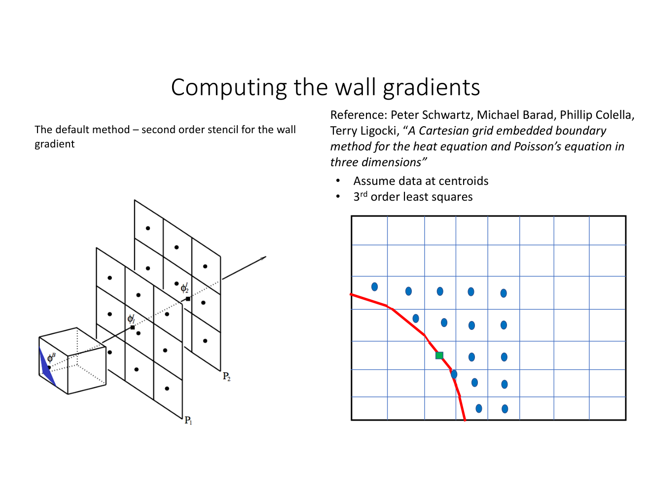
we use a 3rd order least squares formulation to approximate the stress tensor, , at the EB surface. The details of the formulation are given in the Appendix. To determine the gradients on the EB face (green square in Fig. 2), the corresponding least squares formulation results in a linear system of equations at each EB face, given by
For a 3rd order formulation, is a 99 matrix that is dependent only on the mesh in the neighborhood region, is the solution vector that contains the derivatives of variable – first and second (including mixed derivatives), and is a 91 vector which is a function of the values of in the neighborhood region (blue circles in Fig. 2), and the value at the EB face (the green square in Fig. 2). While evaluating gradients of velocity, will take the value of the velocity of the point on the moving body. Note that the values of are assumed to be positioned at the volumetric centroids of the fluid region of the cell (blue circles in Fig. 2). The 9 9 system of equations is solved using LAPACK [5]. In the present work, we use a cluster size of 3, which means that for evaluating the gradients at the EB face on cell , the neighborhood region is given by the reachable fluid-containing cells in the index region .
3 Test cases
Several inviscid and viscous test cases of increasing complexity are performed to validate the numerical method for moving embedded boundaries.
3.1 Harmonically pulsating sphere
This test case is that of a sphere of mean radius m, with a harmonically pulsating surface with radius , with m, and Hz .The pulsation of the sphere creates traveling pressure waves in the surrounding fluid. In the limit of the mean radius of the sphere being small compared to the wavelength corresponding to the acoustic wave with frequency , i.e. , where is the ambient speed of sound, then the pressure perturbation in the domain is given by [77] as
| (9) |
The quiescent ambient condition of the surrounding air (, J/kg K) is given by kg/m3, N/m2. The domain size is m m m, with a base mesh size , and three levels of refinement, that gives a resolution of points across the diameter of the sphere. The velocity of the sphere is surface is given by
where is the outward normal to the spherical surface. Fig. 3 shows the sphere and the three levels of refinement (note that in this and all subsequent test cases presented here, the refinement criteria is set to refine all cut cells in order to avoid intersecting the EB with coarse-fine boundaries. Such intersections are manageable, but would unnecessarily complicate the presentation here.). Fig. 3 shows the instantaneous contours of pressure perturbation on three orthogonal planes through the center of the sphere. Figs. 3 and 3 show the comparison of the numerical and exact solution of pressure perturbation along a radial line that originates at the surface. In this test case, the amplitude of oscillation is small (), and hence the sphere surface does not cut across cells. This test case provides a verification of the correctness of the moving EB flux computation in three dimensions.


3.2 An accelerating piston
This test case demonstrates the classical introduction to shock waves and expansion fans – an accelerating, advancing piston compressing the fluid creates a series of compression waves, the coalescence of which eventually creates a shock wave, and an accelerating, receding piston creates an expansion fan.
3.2.1 Advancing piston
The initial condition consists of quiescent air (, J/kgK) with kg/m3, and N/m2, with the piston located at m. The piston accelerates a constant rate m/s2 at , and hence, the velocity of the piston is given by
which gives the piston motion as
The velocity of the fluid is given as [77]
| (10) |
The location and time of coalescence of compression waves to a shock wave are given by
The domain size is 1 m 0.125 m and the base mesh size is 648 with three levels of refinement. Fig. 4 (a) shows the instantaneous Schlieren () images and the 4-level adaptive mesh. The coalescence of the compression waves to form the shock wave can be seen at ms. The location of the shock m shows good quantitative agreement with the theory. The comparison of the numerical velocity profiles with the exact solution at different time instants is shown in Fig. 4 (b).
 | |
 | |
 |
|
 |
|
 |
|
| (a) | (b) |
3.2.2 Receding piston
The initial condition consists of quiescent air (, J/kgK), with kg/m3, and N/m2, with the piston located at m. The piston accelerates and recedes at a constant rate m/s2 at . The velocity of the fluid is given by Eqn. 10. The domain size is 1 m 0.125 m and the base mesh size is 648 with two levels of refinement. Fig. 5(a) shows the instantaneous velocity contours and the 3-level mesh at various time instants. The comparison of the numerical velocity profiles with the exact solution at different time instants is shown in Fig. 5 (b). This test case creates freshly cleared cells as the piston recedes, and demonstrates the efficiency of our moving boundary formulation.
An expansion fan is a smooth, isentropic flow, and hence the entropy should remain exactly zero at all times. We compute the order of accuracy of the numerical scheme for moving boundary problems using the norm of entropy computed as . Fig. 5(c) shows that the order of accuracy is 1. Although, the numerical scheme has an accuracy of 2 for smooth problems, for moving boundary problems, the order is found to be 1, and is attributed to the interpolation procedure for the freshly cleared cells given by Eqn. 2.1, as has been observed by Muralidharan and Menon 2018 as well.
 | |
 | |
 |
|
 |
|
| (a) | (b) |
 | |
| (c) | |
3.3 Shock-cylinder interaction
To further demonstrate the capability of the moving boundary algorithm we consider the shock-cylinder interaction problem, which has been studied experimentally by Bryson and Gross 1961, and computationally by Bennett et al. 2018. This test case consists of a rigid circular cylinder of diameter m interacting with a stationary Mach 1.34 shock wave. The initial condition corresponds to a stationary shock wave located at m, characterized by the left and right-hand states given by kg/m3, m/s, Pa, and kg/m3, m/s, Pa. The cylinder has a constant horizontal velocity of m/s. The center of the cylinder is initially located at m. The computational domain is 0.18 m 0.18 m with a base mesh size of 32 32, with four levels of refinement, which gives a resolution of 114 points across the diameter of the cylinder. The refinement criterion tags all cut-cells and has an additional gradient based detector for resolving high-gradient regions. The detector at a point is given by Wong and Lele 2016 as
| (11) |
where
If , cells are tagged for refinement. Fig. 6 (a)-(d) shows the evolution of the numerical Schlieren ()
as the cylinder interacts with the shock wave. Since the cylinder moves at the same speed as the surrounding fluid before encountering the shock wave,
the flow-field should not change with time during this period. The absence of any waves in the domain during this time shows that this consistency check is
satisfied by our moving-boundary method similar to Bennett et al. 2018. Fig. 6 shows the mesh at s, and the efficiency of the refinement criterion to
resolve the high gradient regions is evident.
Interaction of a cylinder with a stationary, Mach 2.82 shock wave is done for comparison with experiments of Bryson and Gross 1961. The density and pressure ratios are , and . The initial condition is a shock wave located at m characterized by the left and right states given by kg/m3, m/s, Pa, and kg/m3, m/s, Pa. The cylinder moves with velocity . Fig. 6 shows the comparison of the numerical Schlieren with the experiment of Bryson and Gross 1961. When the incident shock (IS) first impinges on the cylinder, a regular reflected shock (RS) is formed, and later, as the cylinder moves past the incident shock wave, a Mach stem (MS) and a slip surface are formed, that leads to a triple Mach point (TP). The flow features are well resolved with adaptive refinement, and demonstrate qualitatively good comparison with experiments.


3.4 Shock-wedge interaction
In this section, we consider an experimental test case studied by Chang and Chang 2000, known as Schardin’s problem [65] – a Mach 1.34 shock interaction with a triangular wedge. This test case demonstrates the capability of the algorithm to handle high-speed flows around sharp corners. This test case consists of a rigid, equilateral triangular wedge with side length m interacting with a stationary Mach 1.34 shock wave. The initial condition corresponds to a stationary shock wave located at m, characterized by the left and right-hand states given by kg/m3, m/s, Pa, and kg/m3, m/s, Pa. The cylinder has a constant horizontal velocity of m/s. The center of the vertical side of the wedge is initially located at m. The computational domain is 0.09 m 0.09 m with a base mesh size of 32 32, with four levels of refinement. The refinement criterion tags all cut-cells and has an additional gradient based detector for resolving high-gradient regions as described in Section 3.3. Fig. 7-7 show the temporal evolution of the numerical Schlieren (). Fig. 7 shows the 5-level mesh (coarser level is fully refined and hence not seen) showing the effectiveness of the refinement criterion in resolving the high-gradient regions.
Fig. 7 shows the comparison of the experimental [21] and numerical Schlieren images. It can be seen that the various features of the flow are well-resolved and qualitatively match the experimental results. A more detailed Schlieren image of the various features at a later time is shown in Fig. 8. As the wedge interacts with the incident shock wave, a regular reflected shock wave (R) and an expansion fan E are formed initially. As the wedge passes the incident shock the sharp corners lead to the formation of strong vortices (V) and the symmetric decelerated shock wave pattern (D) . At a later time, Mach stems (M1) form on the top and bottom, leading to a triple mach point T1. As the wedge moves forward another Mach stem (M2) originates leading to another triple point (T2).


3.5 Pitching NACA 0012 airfoil
The transonic buffet phenomenon over a NACA 0012 airfoil is widely studied both experimentally [47] and computationally [82, 55, 45, 66]. This test case consists of flow of air (, J/kgK) at Mach 0.755 over a pitching NACA 0012 airfoil with free-stream conditions of kg/m3, m/s and Pa. The pitching motion of the airfoil is about the quarter-chord point , and is defined by the temporally varying angle of attack degrees, with rad/s. A polynomial representation is used to generate the NACA 0012 airfoil [75]. The domain size is 20 m 10 m, and the base mesh size is 256 128 with three levels of refinement. The refinement criterion is defined to tag cut-cells and high gradient regions as defined by Eqn.11.
The flow over the airfoil is transonic as it accelerates over the surface and becomes supersonic, and forms a shock wave which makes it subsonic. Due to the pitching of the airfoil, the shock wave location is unsteady and an oscillating shock wave pattern known as the transonic buffet can be observed over the airfoil. This causes the pressure over the top and bottom surfaces of the airfoil to fluctuate with time, and leads to a cyclic variation of the lift coefficient, and as a result, the lift coefficient has different values as the airfoil encounters the same angle of attack during the upward and downward motion. The transonic buffet phenomenon can be seen in Fig. 9 and 9, which show the contours of Mach number at an angle of attack and respectively. Fig. 9 and 9 show the numerical Schlieren () and the 4-level mesh at and . Fig. 9 shows the comparison of the numerical and experimental [47] pressure coefficient on the top and bottom surfaces of the airfoil at an angle of attack of . Fig. 9 shows the variation of the lift coefficient as a function of the angle of attack. Good quantitative agreement is observed with the experiments of Landon 1982, the numerical simulation of Venkatakrishnan and Mavriplis 1996, and the result from a commercial solver (ANSYS) [55].


3.6 Reciprocating piston in an engine-like geometry
To demonstrate the capability of the algorithm to simulate flows with three dimensional complex, moving geometries, we compute the flow inside the geometry shown in Fig. 10, which mimics an internal combustion engine (without valves). The cross section with the dimensions is shown in Fig. 10. This is a closed system, and hence the mass within the geometry should remain constant with time, which makes this a good case for testing the conservative nature of the scheme. The piston P is initially located at m, and has a prescribed oscillatory motion given by m, which creates a flow within the geometry. The computational domain has dimensions 0.1 m 0.1 m 0.1 m, with a base mesh size of 32 32 32, with two levels of refinement, and a constant time step s is used. The refinement criterion tags all cut-cells for refinement.
Fig. 11-11 show two perpendicular slices with the contours of axial velocity, and the 3-level mesh for different time instants. It can be seen that the geometry is always enclosed within the finest level of refinement. Fig. 11 shows the slices of axial velocity and the 0.5 isocontour of the volume fraction at s. As the piston oscillates, the fluid in the geometry is compressed and expanded, and hence the density changes continuously. Since mass remains constant, the average exact density in the geometry at any time can be computed as , where is the initial mass in the geometry, and is the volume enclosed by a geometry at time . Fig. 11 shows a comparison of the computed and exact average density within the geometry as a function of time over a time period of three cycles of oscillation, which shows good quantitative comparison. To test the conservative nature of the scheme, the percentage error in mass defined as , where , is computed as a function of time for two mesh sizes – and , and shown in Fig. 11. The maximum percentage error is for the mesh is , and reduces to for the mesh. Since the error in mass reduces with refinement, it shows that the algorithm ensures conservation.


3.7 Shock-cone interaction
To demonstrate the capability of the numerical algorithm to simulate high-speed flows with complex geometries and sharp corners in three dimensions, we extend Schardin’s problem described in Section 3.4 to three dimensions, similar to Bennett et al. 2018. This test case consists of a rigid right circular cone of radius m and height m, interacting with a stationary Mach 1.34 shock wave. The domain size is 0.1 m 0.1 m 0.05 m with a base mesh size 32 64 64, with three levels of refinement. The nose of the cone located at m at . The initial condition corresponds to a stationary shock wave located at m, characterized by the left and right-hand states given by kg/m3, m/s, Pa, and kg/m3, m/s, Pa. The cone has a constant horizontal velocity of m/s. . The refinement criterion tags all cut-cells, and has an additional gradient based detector for resolving high-gradient regions.
Fig. 12-12 show the temporal evolution of the numerical Schlieren () on two perpendicular slices. As the cone interacts with the shock, the flow features are noticeably different compared to the shock-wedge interaction case. The high-gradient features evolve spherically, and the interaction of these regions with the strong vortices at the rear of the cone lead to the creation of multiple weak shocks as shown in Fig. 12. Fig. 12 shows the 4-level mesh on the vertical slice showing the effectiveness of the refinement criterion in resolving the high-gradient regions. Fig. 12 shows an instantaneous image of the finest level of refinement, showing the three-dimensional spherical-like nature of the high-gradient regions.


3.8 Horizontally moving cylinder in initially quiescent flow
This test case consists of a horizontally moving cylinder in initially quiescent ambient fluid with kg/m3, kg/ms, at a Reynolds number , based on the cylinder diameter m and cylinder velocity m/s. To evaluate the performance of the moving EB numerical scheme, the pressure and skin friction coefficients over the surface of the cylinder are computed and compared with the results in the literature. The pressure coefficient over the surface of the cylinder is given by , and the skin friction coefficient is given by , where is the shear stress tangential to the surface given by
| (12) |
where and are the components of the surface normal on the body (pointing towards the wall). The domain size is 20 m 10 m, with a base mesh size of 512 256, with 3 levels of refinement, which gives a resolution of 82 points in the cylinder diameter. At , the center of the cylinder is located at . A geometric refinement criterion is used to track the cylinder and its vicinity, which tags all cells in the domain which satisfies and , where are the coordinates of the center of the cylinder at any instant of time. The comparison is performed at a non-dimensional time of . Fig. 13(a)-(c) show the instantaneous contours of velocity magnitude at s, 0.15 s, and 0.3 s. Fig. 14 and 14 show the comparison of the pressure coefficient and skin friction coefficient over the surface of the cylinder respectively. The angle is measured from the stagnation point of the cylinder. Good quantitative comparison is observed, although minor oscillations can be seen in the surface data as has been observed by Al-Marouf and Samtaney 2017.


3.9 Inline oscillating cylinder in initially quiescent flow
A horizontally oscillating cylinder in initially quiescent flow has been widely studied in the literature both experimentally and numerically [28, 39, 3]. The test case consists of a cylinder of diameter D in a quiescent fluid with an imposed oscillatory motion given by
where is the amplitude of oscillation with frequency . The relevant non-dimensional parameters are the Reynolds number , and the Keulegan–Carpenter number , where , is the velocity amplitude attained by the cylinder during the oscillatory motion. Consistent with the test case of Dütsch et al. 1998, we use , which gives m, and , which gives cycles per second. In the current case, m, kg/m3, and kg/ms, which give m, and cycles per second. The domain size is 20 m 10 m, with a base mesh size of 512 256, with 2 levels of refinement, which gives a resolution of 41 points in the cylinder diameter. Since the amplitude of oscillation is small compared to the size of the domain, a static refinement criterion is used, which tags all cells in the domain which satisfies and . Fig. 15 shows the instantaneous contours of vorticity and pressure at various phase positions . As the cylinder oscillates, symmetric vortices develop, and when the direction of oscillation is reversed, the vortex pair gets separated, and a new pair of vortices are formed resulting in a wake reversal as has been observed by Dütsch et al. 1998. Fig. 16 shows the comparison of the normalized velocities in the horizontal and vertical directions at four different streamwise locations given by for different phase positions . The total drag force on the cylinder in the streamwise direction is given by the streamwise component of the force vector
where denotes the surface of the cylinder. Fig. 17 shows the comparison of the drag force over the cylinder as a function of time. The drag force has been normalized to match the results of Dütsch et al. 1998. Good quantitative comparison is observed for all quantities.


3.10 Transversely oscillating cylinder in quiescent flow at Re = 185
A transversely oscillating cylinder in a free stream of initially uniform velocity at various frequencies is a test case that has been widely studied [35]. The vertical position of the cylinder as a function of time is given by
where is the amplitude of oscillation with frequency . The cylinder diameter is m, and the free-stream has pressure N/m2, density kg/m3, flow velocity m/s and viscosity kg/ms, which gives the Reynolds number . The test case is performed for two different oscillation frequencies given by and 1.2, where is the natural frequency of vortex shedding from the cylinder. For , the natural frequency of oscillation, , corresponds to a Strouhal number [83], which gives cycles per second. The domain size is 20 m 10 m, with a base mesh size of 512 256, with 3 levels of refinement, which gives a resolution of 82 points in the cylinder diameter. A geometric refinement criterion is used to the capture the flow features in the vicinity of the cylinder, which tags all cells in the domain which satisfies and . Fig. 18(a)-(d) show the contours of instantaneous vorticity as the cylinder oscillates. The oscillation leads to a cyclic variation of the surface quantities over the cylinder. Fig. 19 (a) and (b) show the comparison of the pressure coefficient over the surface of the cylinder when the cylinder is at the extreme upper position for oscillation frequencies of 0.8 and 1.2 respectively, with the body fitted results of Guilmineau and Queutey 2002. Fig. 20 (a) and (b) show the comparison of the skin friction coefficient , where is the shear stress tangential to the surface given by Eqn. 12. The angle is measured from the stagnation point of the cylinder. Good quantitative comparison is observed, although minor oscillations can be seen.


4 Conclusions
A numerical framework has been developed and validated for the compressible, Navier-Stokes equations involving moving boundaries with an embedded boundary approach within the block-structured adaptive mesh refinement framework of AMReX. The flow solver is developed using a finite volume formulation with a conservative, unsplit, cut-cell approach, and a ghost-cell approach has been developed for computing the inviscid fluxes on the moving, embedded boundary faces. A 3rd order least squares method was used to approximate the gradients of velocities at the EB faces in the computation of the viscous fluxes. The algorithm is validated against analytical and experimental results, and good quantitative comparison is observed. Simulations of shock-cylinder interaction and shock-wedge interaction with adaptive mesh refinement showed the capability of the algorithm to handle high-speed flows with high gradient regions such as shock waves, and flows with sharp corners. The transonic buffet phenomenon of an oscillating NACA 0012 airfoil was simulated, and the variation of the coefficient of lift with the angle of attack showed good quantitative comparison with previous results in literature. As a test of the conservative nature of the scheme, a closed system was simulated – an oscillating piston in a cylinder. The percentage error in mass inside the cylinder was found to decrease with refinement, demonstrating that the scheme is conservative. Viscous test cases of a horizontally moving cylinder, inline oscillating cylinder and a transversely oscillating cylinder were performed, and surface quantities – pressure and skin friction coefficients, were computed and were observed to have good quantitative comparison with results in the literature.
Acknowledgments
This research was supported by the Exascale Computing Project (17-SC-20-SC), a collaborative effort of the U.S. Department of Energy Office of Science and the National Nuclear Security Administration. We also gratefully acknowledge the staff at NREL-HPC for the compute time on the Eagle supercomputer, and their continued support.
Appendix
The idea behind computing gradients at a point (green square in Fig. 2) using the least squares technique is to minimize the cumulative error in the fit to a function over a chosen neighborhood region, with the minimization being done with respect to the gradient quantities at the point in consideration. The value of the function at any point in the neighborhood can be written using a Taylor series expansion about the point at which the gradient needs to be computed. This estimated value will differ from the actual value at the point and the difference between them is the error estimate. The order of the terms retained in the expansion will determine the order of the least squares approximation. For a 3rd order least squares method, the cumulative error that needs to be minimized is given by
where loops over the neighborhood region. In Fig. 2, the neighborhood region consists of the blue circles, which are the centroid of the fluid volumes (the cell containing the face on which the gradient is computed is avoided in the neighborhood region [67]). This error is now minimized with respect to each of the gradient quantities. For eg. gives
which can be rearranged to give
Repeating the above procedure for each of the 9 gradient quantities – , , , , , , , and , gives a 9 9 system of equations as
which is solved using LAPACK [5] to obtain the gradients at the point.
For a 2nd order least squares method, the system of equations is given by
References
- amr [accessed December 5, 2020] AMReX. https://amrex-codes.github.io/amrex/docs_html/, accessed December 5, 2020.
- amr [accessed March 24, 2021] AMReX CNS flow solver. https://github.com/AMReX-Codes/amrex/tree/development/Tests/EB/CNS, accessed March 24, 2021.
- Al-Marouf and Samtaney [2017] Mohamad Al-Marouf and Ravi Samtaney. A versatile embedded boundary adaptive mesh method for compressible flow in complex geometry. Journal of Computational Physics, 337:339–378, 2017.
- Almgren et al. [1997] Ann S Almgren, John B Bell, Phillip Colella, and Tyler Marthaler. A Cartesian grid projection method for the incompressible Euler equations in complex geometries. SIAM Journal on Scientific Computing, 18(5):1289–1309, 1997.
- Anderson et al. [1990] E Anderson, Z Bai, C Bischof, J Demmel, J Dongarra, J DuCroz, A Greenbaum, S Hammarling, A McKenney, and D Sorensen. Lapack: A portable line ar al ge br a li br ary fo r hi g h-pe rfor ma n ce co mput ers. 1990.
- Arrigan et al. [2011] John Arrigan, Vikram Pakrashi, Biswajit Basu, and Satish Nagarajaiah. Control of flapwise vibrations in wind turbine blades using semi-active tuned mass dampers. Structural Control and Health Monitoring, 18(8):840–851, 2011.
- Barton et al. [2011] Philip T Barton, B Obadia, and Dimitris Drikakis. A conservative level-set based method for compressible solid/fluid problems on fixed grids. Journal of Computational Physics, 230(21):7867–7890, 2011.
- Bayyuk et al. [1993] Sami Bayyuk, Kenneth Powell, and Bram VA. A simulation technique for 2-d unsteady inviscid flows around arbitrarily moving and deforming bodies of arbitrary geometry. In 11th Computational Fluid Dynamics Conference, page 3391, 1993.
- Bell et al. [1994] John Bell, Marsha Berger, Jeff Saltzman, and Mike Welcome. Three-dimensional adaptive mesh refinement for hyperbolic conservation laws. SIAM Journal on Scientific Computing, 15(1):127–138, 1994.
- Bennett et al. [2018] WP Bennett, Nikos Nikiforakis, and Rupert Klein. A moving boundary flux stabilization method for Cartesian cut-cell grids using directional operator splitting. Journal of Computational Physics, 368:333–358, 2018.
- Berger and Leveque [1989] Marsha Berger and Randall Leveque. An adaptive Cartesian mesh algorithm for the Euler equations in arbitrary geometries. In 9th Computational Fluid Dynamics Conference, page 1930, 1989.
- Berger and Rigoutsos [1991] Marsha Berger and Isidore Rigoutsos. An algorithm for point clustering and grid generation. IEEE Transactions on Systems, Man, and Cybernetics, 21(5):1278–1286, 1991.
- Berger and Oliger [1984] Marsha J Berger and Joseph Oliger. Adaptive mesh refinement for hyperbolic partial differential equations. Journal of computational Physics, 53(3):484–512, 1984.
- Berger et al. [1989] Marsha J Berger, Phillip Colella, et al. Local adaptive mesh refinement for shock hydrodynamics. Journal of computational Physics, 82(1):64–84, 1989.
- Berger et al. [2003] Marsha J Berger, Christiane Helzel, and Randall J LeVeque. H-box methods for the approximation of hyperbolic conservation laws on irregular grids. SIAM Journal on Numerical Analysis, 41(3):893–918, 2003.
- Berger [1982] MJ Berger. Adaptive mesh refinement for hyperbolic partial differential equations[ph. d. thesis]. 1982.
- Borazjani and Sotiropoulos [2009] Iman Borazjani and Fotis Sotiropoulos. Numerical investigation of the hydrodynamics of anguilliform swimming in the transitional and inertial flow regimes. Journal of Experimental Biology, 212(4):576–592, 2009.
- Brahmachary et al. [2018] Shuvayan Brahmachary, Ganesh Natarajan, Vinayak Kulkarni, and Niranjan Sahoo. A sharp-interface immersed boundary framework for simulations of high-speed inviscid compressible flows. International Journal for Numerical Methods in Fluids, 86(12):770–791, 2018.
- Brown and Henshaw [2000] David L Brown and William D Henshaw. Adaptive mesh refinement routines for overture. Lawrence Livermore National Laboratory Research Report UCRL-MA, 140918, 2000.
- Bryson and Gross [1961] AE Bryson and RWF Gross. Diffraction of strong shocks by cones, cylinders, and spheres. Journal of Fluid Mechanics, 10(1):1–16, 1961.
- Chang and Chang [2000] Se-Myong Chang and Keun-Shik Chang. On the shock–vortex interaction in Schardin’s problem. Shock Waves, 10(5):333–343, 2000.
- Cheny and Botella [2010] Yoann Cheny and Olivier Botella. The ls-stag method: A new immersed boundary/level-set method for the computation of incompressible viscous flows in complex moving geometries with good conservation properties. Journal of Computational Physics, 229(4):1043–1076, 2010.
- Clarke et al. [1986] D Keith Clarke, MD Salas, and HA Hassan. Euler calculations for multielement airfoils using Cartesian grids. AIAA journal, 24(3):353–358, 1986.
- Colella et al. [2006] Phillip Colella, Daniel T Graves, Benjamin J Keen, and David Modiano. A Cartesian grid embedded boundary method for hyperbolic conservation laws. Journal of Computational Physics, 211(1):347–366, 2006.
- DeZeeuw and Powell [1993] Darren DeZeeuw and Kenneth G Powell. An adaptively refined Cartesian mesh solver for the Euler equations. Journal of Computational Physics, 104(1):56–68, 1993.
- Donea et al. [1982] Jean Donea, S Giuliani, and Jean-Pierre Halleux. An arbitrary Lagrangian-Eulerian finite element method for transient dynamic fluid-structure interactions. Computer methods in applied mechanics and engineering, 33(1-3):689–723, 1982.
- Dubey et al. [2014] Anshu Dubey, Ann Almgren, John Bell, Martin Berzins, Steve Brandt, Greg Bryan, Phillip Colella, Daniel Graves, Michael Lijewski, Frank Löffler, et al. A survey of high level frameworks in block-structured adaptive mesh refinement packages. Journal of Parallel and Distributed Computing, 74(12):3217–3227, 2014.
- Dütsch et al. [1998] H Dütsch, F Durst, S Becker, and H Lienhart. Low-reynolds-number flow around an oscillating circular cylinder at low keulegan–carpenter numbers. Journal of Fluid Mechanics, 360:249–271, 1998.
- Fadlun et al. [2000] EA Fadlun, Roberto Verzicco, Paolo Orlandi, and J Mohd-Yusof. Combined immersed-boundary finite-difference methods for three-dimensional complex flow simulations. Journal of computational physics, 161(1):35–60, 2000.
- Fedkiw [2002] Ronald P Fedkiw. Coupling an Eulerian fluid calculation to a lagrangian solid calculation with the ghost fluid method. Journal of Computational Physics, 175(1):200–224, 2002.
- Fedkiw et al. [1999] Ronald P Fedkiw, Tariq Aslam, Barry Merriman, Stanley Osher, et al. A non-oscillatory Eulerian approach to interfaces in multimaterial flows (the ghost fluid method). Journal of computational physics, 152(2):457–492, 1999.
- Forrer and Berger [1999] Hans Forrer and Marsha Berger. Flow simulations on Cartesian grids involving complex moving geometries. In Hyperbolic problems: theory, numerics, applications, pages 315–324. Springer, 1999.
- Gilmanov and Sotiropoulos [2005] Anvar Gilmanov and Fotis Sotiropoulos. A hybrid Cartesian/immersed boundary method for simulating flows with 3d, geometrically complex, moving bodies. Journal of computational physics, 207(2):457–492, 2005.
- Goldstein et al. [1993] D Goldstein, R Handler, and L Sirovich. Modeling a no-slip flow boundary with an external force field. Journal of computational physics, 105(2):354–366, 1993.
- Guilmineau and Queutey [2002] Emmanuel Guilmineau and P Queutey. A numerical simulation of vortex shedding from an oscillating circular cylinder. Journal of Fluids and Structures, 16(6):773–794, 2002.
- Hartmann et al. [2009] Daniel Hartmann, Matthias Meinke, and Wolfgang Schröder. A general formulation of boundary conditions on Cartesian cut-cells for compressible viscous flow. In 19th AIAA Computational Fluid Dynamics, page 3878. 2009.
- Hu et al. [2006] Xiangyu Y Hu, BC Khoo, Nikolaus A Adams, and FL Huang. A conservative interface method for compressible flows. Journal of Computational Physics, 219(2):553–578, 2006.
- Hughes et al. [1981] Thomas JR Hughes, Wing Kam Liu, and Thomas K Zimmermann. Lagrangian-Eulerian finite element formulation for incompressible viscous flows. Computer methods in applied mechanics and engineering, 29(3):329–349, 1981.
- Iliadis and Anagnostopoulos [1998] G Iliadis and Petros Anagnostopoulos. Viscous oscillatory flow around a circular cylinder at low keulegan–carpenter numbers and frequency parameters. International Journal for Numerical Methods in Fluids, 26(4):403–442, 1998.
- Ji et al. [2010] Hua Ji, Fue-Sang Lien, and Eugene Yee. Numerical simulation of detonation using an adaptive Cartesian cut-cell method combined with a cell-merging technique. Computers & fluids, 39(6):1041–1057, 2010.
- Johansen and Colella [1998] Hans Johansen and Phillip Colella. A Cartesian grid embedded boundary method for Poisson’s equation on irregular domains. Journal of Computational Physics, 147(1):60–85, 1998.
- Kern and Koumoutsakos [2006] Stefan Kern and Petros Koumoutsakos. Simulations of optimized anguilliform swimming. Journal of Experimental Biology, 209(24):4841–4857, 2006.
- Khalili et al. [2018] M Ehsan Khalili, Martin Larsson, and Bernhard Müller. Immersed boundary method for viscous compressible flows around moving bodies. Computers & Fluids, 170:77–92, 2018.
- Kirkpatrick et al. [2003] MP Kirkpatrick, SW Armfield, and JH Kent. A representation of curved boundaries for the solution of the Navier–Stokes equations on a staggered three-dimensional Cartesian grid. Journal of Computational Physics, 184(1):1–36, 2003.
- Kirshman and Liu [2006] DJ Kirshman and F Liu. Flutter prediction by an Euler method on non-moving Cartesian grids with gridless boundary conditions. Computers & fluids, 35(6):571–586, 2006.
- Klein et al. [2009] R Klein, KR Bates, and N Nikiforakis. Well-balanced compressible cut-cell simulation of atmospheric flow. Philosophical Transactions of the Royal Society A: Mathematical, Physical and Engineering Sciences, 367(1907):4559–4575, 2009.
- Landon [1982] RH Landon. NACA 0012 oscillating and transient pitching, data set 3 in AGARD-R-702, compendium of unsteady aerodynamic measurements. Report, August, 1982.
- LeVeque [1988] Randall J LeVeque. Cartesian grid methods for flow in irregular regions. Numerical Methods in Fluid Dynamics, 3:375–382, 1988.
- Liu and Kawachi [1998] Hao Liu and K Kawachi. A numerical study of insect flight. Journal of computational physics, 146(1):124–156, 1998.
- Liu et al. [2003] TG Liu, BC Khoo, and KS Yeo. Ghost fluid method for strong shock impacting on material interface. Journal of computational physics, 190(2):651–681, 2003.
- Meyer et al. [2010] Michael Meyer, A Devesa, Stefan Hickel, XY Hu, and Nikolaus A Adams. A conservative immersed interface method for large-eddy simulation of incompressible flows. Journal of Computational Physics, 229(18):6300–6317, 2010.
- Mittal et al. [2008] Rajat Mittal, Haibo Dong, Meliha Bozkurttas, FM Najjar, Abel Vargas, and Alfred Von Loebbecke. A versatile sharp interface immersed boundary method for incompressible flows with complex boundaries. Journal of computational physics, 227(10):4825–4852, 2008.
- Modiano and Colella [2000] D Modiano and P Colella. A higher-order embedded boundary method for time-dependent simulation of hyperbolic conservation laws. Technical report, Lawrence Berkeley National Lab.(LBNL), Berkeley, CA (United States), 2000.
- Mohd-Yusof [1997] Jamaludin Mohd-Yusof. Combined immersed-boundary/b-spline methods for simulations of flow in complex geometries. Center for turbulence research annual research briefs, 161(1):317–327, 1997.
- Mumtaz et al. [2017] Muhammad Saleem Mumtaz, Adnan Maqsood, and Salma Sherbaz. Computational modeling of dynamic stability derivatives for generic airfoils. In MATEC Web of Conferences, volume 95, page 12006. EDP Sciences, 2017.
- Muralidharan [2017] Balaji Muralidharan. An embedded boundary approach for simulation of reacting flow problems in complex geometries with moving and stationary boundaries. PhD thesis, Georgia Institute of Technology, 2017.
- Muralidharan and Menon [2016] Balaji Muralidharan and Suresh Menon. A high-order adaptive Cartesian cut-cell method for simulation of compressible viscous flow over immersed bodies. Journal of Computational Physics, 321:342–368, 2016.
- Muralidharan and Menon [2018] Balaji Muralidharan and Suresh Menon. Simulation of moving boundaries interacting with compressible reacting flows using a second-order adaptive Cartesian cut-cell method. Journal of Computational Physics, 357:230–262, 2018.
- Noh [1963] William F Noh. Cel: A time-dependent, two-space-dimensional, coupled Eulerian-Lagrange code. Technical report, Lawrence Radiation Lab., Univ. of California, Livermore, 1963.
- Pember et al. [1995] Richard B Pember, John B Bell, Phillip Colella, William Y Curtchfield, and Michael L Welcome. An adaptive Cartesian grid method for unsteady compressible flow in irregular regions. Journal of computational Physics, 120(2):278–304, 1995.
- Peskin [1972] Charles S Peskin. Flow patterns around heart valves: a numerical method. Journal of computational physics, 10(2):252–271, 1972.
- Popinet [2003] Stéphane Popinet. Gerris: a tree-based adaptive solver for the incompressible Euler equations in complex geometries. Journal of Computational Physics, 190(2):572–600, 2003.
- Quirk [1994] James J Quirk. A Cartesian grid approach with hierarchical refinement for compressible flows. Technical report, Institute for Computer Applications In Science and Engineering, Hampton, Virginia, 1994.
- Sahin and Mohseni [2009] Mehmet Sahin and Kamran Mohseni. An arbitrary Lagrangian–Eulerian formulation for the numerical simulation of flow patterns generated by the hydromedusa aequorea victoria. Journal of Computational Physics, 228(12):4588–4605, 2009.
- Schardin [1957] H Schardin. High frequency cinematography in the shock tube. The Journal of Photographic Science, 5(2):17–19, 1957.
- Schneiders et al. [2013] Lennart Schneiders, Daniel Hartmann, Matthias Meinke, and Wolfgang Schröder. An accurate moving boundary formulation in cut-cell methods. Journal of Computational Physics, 235:786–809, 2013.
- Schwartz et al. [2006] Peter Schwartz, Michael Barad, Phillip Colella, and Terry Ligocki. A Cartesian grid embedded boundary method for the heat equation and Poisson’s equation in three dimensions. Journal of Computational Physics, 211(2):531–550, 2006.
- Sharan et al. [2020] Nek Sharan, Peter T Brady, and Daniel Livescu. Stable and conservative boundary treatment for difference methods, with application to cut-cell discretizations. In AIAA Scitech 2020 Forum, page 0807, 2020.
- Steger et al. [1983] Joseph L Steger, F Carroll Dougherty, and John A Benek. A chimera grid scheme.[multiple overset body-conforming mesh system for finite difference adaptation to complex aircraft configurations]. 1983.
- Stout et al. [1997] Quentin F Stout, Darren L De Zeeuw, Tamas I Gombosi, Clinton Groth, Hal G Marshall, and Kenneth G Powell. Adaptive blocks: A high performance data structure. In Proceedings of the 1997 ACM/IEEE conference on Supercomputing, pages 1–10. ACM, 1997.
- Su et al. [2007] Shen-Wei Su, Ming-Chih Lai, and Chao-An Lin. An immersed boundary technique for simulating complex flows with rigid boundary. Computers & fluids, 36(2):313–324, 2007.
- Tan and Shu [2010] Sirui Tan and Chi-Wang Shu. Inverse lax-wendroff procedure for numerical boundary conditions of conservation laws. Journal of Computational Physics, 229(21):8144–8166, 2010.
- Tan and Shu [2011] Sirui Tan and Chi-Wang Shu. A high order moving boundary treatment for compressible inviscid flows. Journal of Computational Physics, 230(15):6023–6036, 2011.
- Terashima and Tryggvason [2009] Hiroshi Terashima and Grétar Tryggvason. A front-tracking/ghost-fluid method for fluid interfaces in compressible flows. Journal of Computational Physics, 228(11):4012–4037, 2009.
- Tools [2015] Airfoil Tools. Naca 4 digit airfoil generator. National Advisory Committee for Aeronautics, 2015.
- Toro [2013] Eleuterio F Toro. Riemann solvers and numerical methods for fluid dynamics: a practical introduction. Springer Science & Business Media, 2013.
- Tsangaris and Pappou [2000] S Tsangaris and Th Pappou. Analytical solutions for the unsteady compressible flow equations serving as test cases for the verification of numerical schemes. Technical report, Laboratory of Aerodynamics, National Technical University of Athens, 2000.
- Tseng and Ferziger [2003] Yu-Heng Tseng and Joel H Ferziger. A ghost-cell immersed boundary method for flow in complex geometry. Journal of computational physics, 192(2):593–623, 2003.
- Udaykumar et al. [1996] HS Udaykumar, Wei Shyy, and MM Rao. Elafint: a mixed Eulerian–Lagrangian method for fluid flows with complex and moving boundaries. International journal for numerical methods in fluids, 22(8):691–712, 1996.
- Udaykumar et al. [1999] HS Udaykumar, Rajat Mittal, and Wei Shyy. Computation of solid–liquid phase fronts in the sharp interface limit on fixed grids. Journal of computational physics, 153(2):535–574, 1999.
- Uhlmann [2005] Markus Uhlmann. An immersed boundary method with direct forcing for the simulation of particulate flows. Journal of Computational Physics, 209(2):448–476, 2005.
- Venkatakrishnan and Mavriplis [1996] V Venkatakrishnan and DJ Mavriplis. Implicit method for the computation of unsteady flows on unstructured grids. Journal of Computational Physics, 127(2):380–397, 1996.
- Williamson and Brown [1998] CHK Williamson and GL Brown. A series in 1/ to represent the strouhal–reynolds number relationship of the cylinder wake. Journal of Fluids and Structures, 12(8):1073–1085, 1998.
- Wong and Lele [2016] Man Long Wong and Sanjiva K Lele. Multiresolution feature detection in adaptive mesh refinement with high-order shock-and interface-capturing scheme. In 46th AIAA Fluid Dynamics Conference, page 3810, 2016.
- Yang et al. [1997a] G Yang, DM Causon, DM Ingram, R Saunders, and P Battent. A Cartesian cut cell method for compressible flows part a: Static body problems. The Aeronautical Journal, 101(1002):47–56, 1997a.
- Yang et al. [1997b] G Yang, DM Causon, DM Ingram, R Saunders, and P Battent. A Cartesian cut cell method for compressible flows part b: moving body problems. The Aeronautical Journal, 101(1002):57–65, 1997b.
- Yang et al. [2000] G Yang, DM Causon, and DM Ingram. Calculation of compressible flows about complex moving geometries using a three-dimensional Cartesian cut cell method. International Journal for Numerical Methods in Fluids, 33(8):1121–1151, 2000.
- Yang and Balaras [2006] Jianming Yang and Elias Balaras. An embedded-boundary formulation for large-eddy simulation of turbulent flows interacting with moving boundaries. Journal of Computational Physics, 215(1):12–40, 2006.
- Ye et al. [1999] Tao Ye, Rajat Mittal, HS Udaykumar, and Wei Shyy. An accurate Cartesian grid method for viscous incompressible flows with complex immersed boundaries. Journal of computational physics, 156(2):209–240, 1999.
- Zhang et al. [2019] Weiqun Zhang, Ann Almgren, Vince Beckner, John Bell, Johannes Blaschke, Cy Chan, Marcus Day, Brian Friesen, Kevin Gott, Daniel Graves, Max Katz, Andrew Myers, Tan Nguyen, Andrew Nonaka, Michele Rosso, Samuel Williams, and Michael Zingale. AMReX: a framework for block-structured adaptive mesh refinement. Journal of Open Source Software, 4(37):1370, May 2019. doi: 10.21105/joss.01370. URL https://doi.org/10.21105/joss.01370.