DCT2net: an interpretable shallow CNN for image denoising

In its most mature formulation for image denoising [1], the DCT denoiser proceeds on small overlapping patches accross the image. Each patch of size $p\times p$ is denoised independently, so that each pixel is in fact denoised $p^{2}$ times. For each pixel, the final denoised value is then obtained by averaging those $p^{2}$ estimators. Typical values for $p$ are powers of $2$ (generally $8$ or $16$) for practical reasons in the computation of the fast discrete cosine transform. However, we focus here on the case where $p$ is an odd number, without loss of generality.

For the sake of representation, we denote by $\boldsymbol{y}_{k,p}^{i,j}$ the $p\times p$ patch, in the vector form, for which the central pixel, is located $j$ pixels at the right of the $k^{th}$ pixel of $\boldsymbol{y}$ and $i$ pixels beneath it (see Fig. 1). Note that $i$ and $j$ can be negative numbers. Let us denote $q=\lfloor\frac{p}{2}\rfloor$ (i.e. closest integer less than or equal to $p/2$). The DCT denoiser denoted $F$ can then be expressed as:

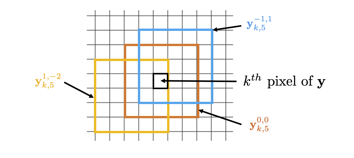
By definition of DCT, the mathematical expression of the coefficient of the matrix $\boldsymbol{P}$ at row $i=xp+y+1$ and column $j=up+v+1$ for $(x,y,u,v)\in\llbracket 0,p-1\rrbracket^{4}$ is given by:

A small improvement of [1], called adaptive aggregation and inspired from [7], was proposed in [26]. The idea is to give higher weight to patches that have a sparser representation in the DCT domain, enabling to reduce the ringing effects near edges. The expression of the improved DCT denoiser then becomes:

Interestingly, one of the easiest implementation of a DCT denoiser, as formulated in (3), can be done with a neural network. Indeed, all operations involved can be interpreted in terms of convolutions with a hard shrinkage function as activation function.

Our shallow CNN is first composed of a convolutional layer with kernel size $p\times p$ leading to $p^{2}$ output channels. Figure 2 shows such an architecture when $p=5$. Note that the weights involved in kernels are to be found in the matrix $\boldsymbol{P}^{-1}$: each row is associated with one convolutional kernel. The action of this layer can be summed up as follows: each pixel is replaced by the patch formed by its neighborhood, after transformation by $\boldsymbol{P}^{-1}$. Then, the hard shrinkage function is applied element-wise. Afterwards, a $1\times 1$ convolution layer operates on those patches where the weights correspond to the elements of the matrix $\boldsymbol{P}$. In order to compute the adaptive aggregation, we have to generate a weight map from the first layer computing the values $w_{i,j,k}$ in (3). This latter is used to balance the features resulting from the second layer by channel-wise multiplication. The weighted pixels are then repositioned at their corresponding locations and then aggregated by summation. This can be implemented with the help of a last convolutional layer where the values of weights are either $0$ or $1$. Note that, for computational efficiency, a 2D transposed convolution is recommended. Finally, a normalization by $W_{k}$ (see (3)) is performed by dividing the last layer by the weight map, beforehand convolved by a kernel composed of ones.

We want to stress that our DCT2net is the strict implementation of the formulation in (3). Equipped with the correct weights given by the definition of the DCT in (2), it exactly produces the same results as those obtained with the traditional implementation.

As it is usually done with neural networks, we can train our DCT2net on an external dataset composed of $N$ pairs of noise-free and noisy images $(\boldsymbol{x}_{i},\boldsymbol{y}_{i})_{i\in\{1,\ldots,N\}}$ to improve the underlying transform. More precisely, our objective is to solve the following optimization problem:

To that extent, we need to restrict the model to the original transform where only one matrix is involved (the other one being its inverse) and where the other convolutions of the network composed of $0$ and $1$ are frozen. This can be achieved with the help of modern machine learning libraries such as Pytorch for which automatic differentiation can be kept on for complex operations such as matrix inversion but also deactivated for some layers. Nevertheless, the thresholding operation must be slightly adapted in a context of gradient descent where differentiation is needed. Thus, we replace the function $\boldsymbol{1}_{\mathbb{R}\backslash[-\lambda,\lambda]}$ by $\zeta_{m,\lambda}(x)=\frac{x^{2m}}{x^{2m}+\lambda^{2m}}$ with $m\in\mathbb{N}^{*}$. This choice is legitimate as the sequence of functions $(\zeta_{m,\lambda})_{m\in\mathbb{N}^{*}}$ converges pointwise to $\boldsymbol{1}_{\mathbb{R}\backslash[-\lambda,\lambda]}$. The hard shrinkage function $\varphi_{\lambda}$ then becomes $\varphi_{m,\lambda}(x)=\frac{x^{2m+1}}{x^{2m}+\lambda^{2m}}$. Figure 3 shows how close this approximation is from the original hard shrinkage function with ever growing values of $m$. By the way, this approximation is adopted only during the training phase for facilitating the optimization process. To stick with the original DCT denoiser, we use the original hard shrinkage function for the testing phase that gives the same results in terms of PSNR with no noticeable visual differences for the denoised images. It is worth noting that the use of the original hard shrinkage function instead of our differentiable approximation for the training phase does not work in our case, leading to a poor suboptimal local minimum, even though this activation function is available in most modern machine learning libraries. It is likely that this disappointing behavior is due to the discontinuity of the original function.

Finally, as recommended in [1], the threshold parameter $\lambda$ is set to $3\sigma$ to significantly remove noise. But the choice of the multiplicative constant in front of $\sigma$ is actually of little importance and any other constant would produce same results as long as $\boldsymbol{P}$ can adapt itself. Indeed, for two levels of threshold $\lambda$ and $\lambda^{\prime}$, we have $\varphi_{\lambda}(x)=\frac{\lambda}{\lambda^{\prime}}\varphi_{\lambda^{\prime}}(\frac{\lambda^{\prime}}{\lambda}x)$. In particular, for two choices of multiplicative constant $c$ and $c^{\prime}$, $\varphi_{c\sigma}(x)=\frac{c}{c^{\prime}}\varphi_{c^{\prime}\sigma}(\frac{c^{\prime}}{c}x)$, hence $\boldsymbol{P}\varphi_{c\sigma}(\boldsymbol{P}^{-1}\boldsymbol{y})=\boldsymbol{Q}\varphi_{c^{\prime}\sigma}(\boldsymbol{Q}^{-1}\boldsymbol{y})$ with $\boldsymbol{Q}=\frac{c}{c^{\prime}}\boldsymbol{P}$ This means that, in theory, choosing a value other than $3$ would result in estimating the same transform, up to a multiplicative constant, and with exactly the same denoising performance. Appendix A gives more details about the choice of threshold, studying more particularly the case where multiple thresholds are used.

Note that, in practice, optimizing over the set of invertible matrices $\mathcal{GL}_{p^{2}}(\mathbb{R})$ in (4) is not an issue and the problem can be treated through stochastic gradient descent without specific precaution. It is attributable to the fact that $\mathcal{GL}_{p^{2}}(\mathbb{R})$ is dense in $\mathcal{M}_{p^{2}}(\mathbb{R})$ but $\mathcal{M}_{p^{2}}(\mathbb{R})\backslash\mathcal{GL}_{p^{2}}(\mathbb{R})$ is not.

In the definition of DCT2net (3), we impose no orthonormality constraint to learn the basis. Therefore, it is no wonder that, during the building of the matrix $\boldsymbol{P}$ through stochastic gradient descent, the property of orthonormality gets lost. One way ¹¹ 1 For a direct technique to derive an orthonormal matrix, with similar results compared to the regularization form, see appendix B. to address this issue is to add a regularization term that encourages orthonormality in the optimization process. The problem amounts to solving:

It is worth noting that the resulting matrix $\boldsymbol{P}^{*}$ is not guaranteed to be orthonormal whatever the parameter $\beta$ is. To derive an orthonormal matrix from $\boldsymbol{P}^{*}$, we can select its nearest orthonormal matrix $\boldsymbol{P}_{\text{ortho}}$ in the Frobenius norm sense. The unique solution is given by $\boldsymbol{P}_{\text{ortho}}=\boldsymbol{U}\boldsymbol{V}^{T}$ where $\boldsymbol{U}$ and $\boldsymbol{V}$ are the matrices from the singular value decomposition of $\boldsymbol{P}^{*}=\boldsymbol{U}\boldsymbol{\Sigma}\boldsymbol{V}^{T}$.

However, adding a constraint of orthonormality limits the expressivity of the network and we observed that the denoising performance was not as good as the regularization-free solution (see Fig. 5). Moreover, the choice of the regularization parameter $\beta$ can be challenging as it needs to be adapted for each patch size. For all those reasons, we decided not to retain a solution with an orthonormal matrix. In spite of this, the matrix $\boldsymbol{P}$ learned by DCT2net is quite close to be orthogonal, even if no constraint has been imposed. This is illustrated in Fig. 6 which displays the matrix $\boldsymbol{P}^{T}\boldsymbol{P}$ for patches of size $9\times 9$. We can notice that the non-diagonal elements are close to zero, which is expected for a matrix close to be orthogonal. In appendix C, we show how orthogonal and orthonormal matrices are linked, stating that if $\boldsymbol{P}$ is orthogonal, there exists an orthonormal matrix $\boldsymbol{Q}$ that would give exactly the same results in DCT2net as long as we set a different threshold by element of the basis.

Finally, as regards the initialization for the stochastic gradient descent, the original DCT basis (see (2)) is considered by default. Considering random initializations such as Xavier initialization which is common in deep neural networks, lead to similar bases, even though the time for convergence is slightly more important. The convergence to the same solution whatever the initialization is a very good news, suggesting that optimizing the underlying non-convex problem is tractable.

When displaying the learned basis on a popular image dataset such as BSD400 [27], one may be surprised. Interestingly, this basis, in which each patch is decomposed, is much more disorganized than the original DCT basis. One may doubt that the DCT2net basis denoises better patches as it contains no clear pattern. As a matter of fact, applying this basis does not denoise patches but rather degrades them even more as shown in Fig. 7. The main reason is that the network actually denoise image patches and performs aggregation at once, making it difficult to understand why such a basis improves the PSNR value of the restored image.

We observed that, for a given noisy pixel $k$ belonging to $p^{2}$ patches, the $p^{2}$ ”denoised” versions of pixel $k$ with DCT2net have a very high variance when compared to the $p^{2}$ denoised values obtained with the DCT denoiser, for which all $p^{2}$ denoised values are generally almost all the same, as illustrated in Fig. 7. Nevertheless, after the adaptive aggregation step, the pixels denoised by applying the learned transform are closer, in average, to the ground truth ones. This is a counter-intuitive result that questions our preconceptions on denoising. This suggests that the final aggregation step is not a basic post-processing step but plays an important role in denoising, as confirmed below.

As the strategy followed by DCT2net is counter-intuitive and hardly comprehensible for a human brain, we tried to constrain the learned transform to effectively denoise patches. In this study, aggregation is performed in a second step with conventional weighted averages. This can be done in practice by cutting our neural network represented in Fig. 2 after the two first convolutional layers, so that the output $F_{\boldsymbol{P}}(\boldsymbol{y}_{i})$ is of size $(H-p+1)\times(W-p+1)\times p^{2}$. For a clean image $\boldsymbol{x}_{i}$, we can compute its patch representation $\Pi(\boldsymbol{x}_{i})$ of size $(H-p+1)\times(W-p+1)\times p^{2}$ as well and solve the following optimization problem:

Figure 4e shows the learned transform $\boldsymbol{P}^{*}$ that effectively denoise patches. The resulting matrix $\boldsymbol{P}^{*}$ is much more natural and interestingly very close the original DCT basis. The gain in PSNR on patches of this new transform was evaluated on the Set 12 dataset. The results reported in Table I show that the learned transform produces systematically a higher PSNR in average for the patches than the traditional DCT. One could expect that this transform would outperform DCT after the aggregation step. Unfortunately, this is not the case. Once the transform has been re-used in our DCT2net shown in Fig. 2 with the adaptive aggregation integrated, the expected boost compared to traditional DCT in terms of PSNR significantly decreases. The difference of PSNR is insignificant, with a visually less attractive result. We can notice an interesting phenomenon for $\sigma=15$: from better denoised patches, our learned transform fails to outperform the traditional DCT after any classical aggregation technique. This counter-intuitive result confirms, once again, that the aggregation step is equally important as denoising patches.

To go beyond DCT, the key issue is to follow a non-intuitive path that consists in degrading the patches and performing aggregation step to rearrange everything and produce a high-quality denoised image.

We trained our DCT2net on 400 gray-scale images from the Berkeley segmentation dataset (BSDS) [27] where synthetic Gaussian noise with zero mean and a random standard deviation $\sigma$ taken in $\in[1,55]$ was added in order to create our pairs $(\boldsymbol{x}_{i},\boldsymbol{y}_{i})_{i\in\{1,\ldots,N\}}$ with $N\gg 400$ (the $\boldsymbol{x}_{i}$ are redundant). Contrary to numerous deep learning models, our network can adapt to the level of noise as the differentiable hard shrinkage function depends on $\sigma$, so that we train our model only once for all levels of noise at the same time.

During training, we randomly sample cropped images from the training set of size $128\times 128$ with a mini-batch size of $32$. We use horizontal and vertical flipping as well as random rotations $\in\{0^{\circ},90^{\circ},180^{\circ},270^{\circ}\}$ as further data augmentation. In total, $400\times 665$ overlapping patches from $400$ clean images are used for training. The mean squared error was used as loss function and we used Adam optimizer [28]. The learning rate was set to $10^{-3}$ and decreased exponentially to $10^{-5}$ during the $15$ epochs required for convergence. Note that we initialized the weights of our networks according to the original discrete cosine transform given by (2). Initializing the weights randomly, for example with a Xavier initialization as it is usually done with deep neural networks, only slows down the time for convergence. As for the parameter $m$ specifying the degree of approximation of the hard shrinkage function $\varphi_{\lambda}$, we took $m=32$. Training a model took approximately 8 hours with a GeForce RTX 2080 Ti.

Note that a small improvement of our hybrid solution DCT/DCT2net can be obtained by training DCT2net only on parts of images where the learned transform will be applied. In practice, this is done by pre-computing binary masks $b_{i}$ according to the classification proposed for every image of the external dataset and solving:

We recall the parameters chosen for the Canny edge detector: lower and upper thresholds are set once and for all respectively to $0.1$ and $0.2$ and a supplementary dilation operation is performed using a kernel of size $5\times 5$.

We tested the denoising performance of our architecture on two well-known datasets: Set 12 and BSD68. According to our experiments, the best model for DCT/DCT2net in terms of performance (i.e., PSNR) and subjective visual quality is obtained with a patch size of $13$. Larger sizes of patch only bring negligible enhancement for a complexity much more important.

Tables III and IV compare the performance of traditional and deep-learning-based state-of-the-art algorithms with our model. We compare our DCT2net with BM3D [7] and PEWA [11], both state-of-the-art traditional methods that exploit self-similarity and DCT decomposition. We also compare DCT2net to related algorithm Deep K-SVD [22]. Scetbon et al. [22] proposed multiple models that depend on the patch size, the dictionary size and the number of denoising steps. In what follows, we consider the smallest model for which an implementation is given by the authors and which is denoted LKSVD_1,8,256. We performed the training by ourselves for each noise level, as no pretrained models were supplied by the authors.

We can notice that DCT2net achieves comparable performances with state-of-the-art traditional algorithms on both Set12 and BSD68 datasets, outperforming its original counterpart DCT²² 2 The non-adaptive version of DCT denoiser was considered as it produced a slightly higher PSNR, despite its poor subjective visual quality. [1]. Unlike BM3D and PEWA and other algorithms such as NL-Bayes [9], DCT2net is a very simple one-pass algorithm, able to produce similar performances to Deep K-SVD for high noise level while it is not trained specifically to address such challenging situations.

Beyond the performance assessed with the PSNR criterion, nothing can replace the subjective assessment of a human eye. On this criterion, our DCT/DCT2net can hold its own against established methods such as BM3D as shown in Figure 12. The use of the traditional DCT on flat areas produces, for example, a better-looking sky than Deep K-SVD or BM3D when applied to the Castle image. Unsurprisingly, DCT/DCT2net (based on two layers) cannot compete with very deep neural networks such that DnCNN [15] but it is faster (see below and Table V).

Nevertheless, the performance has to be put in perspective with the complexity of the model which is studied in the next subsection.

We want to emphasize that DCT2net is very light and fast compared to its traditional and deep-learning-based counterparts. In Table VI, we reported the complexity in terms of layers numbers and parameters. The number of parameters of DCT2net represents only 5% of the total of parameters of DnCNN. Moreover, the underlying parameters are the same whatever the noise level is, which is not the case for DnCNN or Deep K-SVD where the models have to be trained from scratch for every noise level³³ 3 Although solutions for handling multiple noise levels within the same network were proposed, including a noisemap at the network entry by the authors of [16].

In addition to the number of parameters, the executing time is a crucial feature of denoising algorithms. Table V is provided for information purposes only, as the implementation, the language used and the machine on which the code is run, highly influence the execution time. The CPU used is a 2,3 GHz Intel Core i7 and the GPU is a GeForce RTX 2080 Ti. We used the IPOL implementation [29] for BM3D [7] and the implementation provided by the authors for the others algorithms, except for DCT [1] that we re-implemented with Pytorch on our own, leveraging the network unfolding scheme already used in [22]. By the way, DCT2net can be easily adapted to this specific unfolding implementation, as there is no difference between DCT2net and DCT denoiser, apart from the underlying bases.

We also tried to train our network on fewer images than the original BSD400 dataset. As our network relies on a two-layers architecture, it is less prone to overfitting and the learning can be performed only from several dozens of images. With 10 and 40 images, corresponding to $10\times 665$ and $40\times 665$ overlapping patches of size $128\times 128$ respectively, our DCT/DCT2net achieves almost the same performance with no visual difference. By way of comparison, training a model with 40 images takes less than one hour with a GeForce RTX 2080 Ti and the average PSNR values on Set12 are 32.07dB, 29.69dB and 26.39dB, for $\sigma=15$, $25$ and $50$ respectively.

References

- [1] G. Yu and G. Sapiro, “DCT image denoising: a simple and effective image denoising algorithm,” in Image Processing On Line, vol. 1, pp. 292–296, 2011.
- [2] H. Chipman, E. Kolaczyk, and R. McCulloch, “Adaptive Bayesian Wavelet Shrinkage,” in Journal of the American Statistical Association, vol. 92, no. 440, pp. 1413-1421, 1997.
- [3] W. B. Pennebaker and J. L. Mitchell, “JPEG: still image data compression standard,” Van Nostrand Reinhold, New York, 1992.
- [4] M. Elad and M. Aharon, “Image denoising via sparse and redundant representations over learned dictionaries,” in IEEE Transactions on Image Processing, vol. 15, no. 12, pp. 3736-3745, 2006.
- [5] A. Buades, B. Coll, and J.-M. Morel, “A review of image denoising algorithms, with a new one,” in SIAM Journal on Multiscale Modeling and Simulation, vol. 4, no. 2, pp. 490-530, 2005.
- [6] M. Zontak and M. Irani, “Internal statistics of a single natural image,” in IEEE Conference on Computer Vision and Pattern Recognition (CVPR), Colorado Springs, CO, USA, 2011, pp. 977-984.
- [7] K. Dabov, A. Foi, V. Katkovnik, and K. Egiazarian, “Image denoising by sparse 3D transform-domain collaborative filtering,” in IEEE Transactions on Image Processing, vol. 16, no. 8, pp. 2080–2095, 2007.
- [8] J. Mairal, F. Bach, J. Ponce, G. Sapiro, and A. Zisserman, “Non-local sparse models for image restoration,” in IEEE 12th International Conference on Computer Vision, Tokyo, Japan, 2009, pp. 2272-2279.
- [9] A. Buades, M. Lebrun, and J.-M. Morel. “A Non-local Bayesian image denoising algorithm,” in SIAM Journal on Imaging Science, vol. 6, no. 3, pp. 1665-1688, 2013.
- [10] S. Gu, L. Zhang, W. Zuo, and X. Feng, “Weighted Nuclear Norm Minimization with Application to Image Denoising,” in IEEE Conference on Computer Vision and Pattern Recognition, Columbus, OH, USA, 2014, pp. 2862-2869.
- [11] C. Kervrann, “PEWA : Patch-based exponentially weighted aggregation for image denoising,” in Neural Information Processing Systems, Montreal, Canada, 2014, pp. 2150–2158.
- [12] Q. Jin, I. Grama, C. Kervrann, and Q. Liu, “Non-local means and optimal weights for noise removal,” in SIAM Journal on Imaging Sciences, vol. 10, no. 4, pp. 1878-1920, 2017.
- [13] C. Kervrann and J. Boulanger, “Optimal spatial adaptation for patch-based image denoising,” in IEEE Transactions on Image Processing, vol. 15, no. 10, pp. 2866-2878, 2006.
- [14] C. Kervrann and J. Boulanger, “Local adaptivity to variable smoothness for exemplar-based image denoising and representation,” in International Journal of Computer Vision, vol. 79, no. 1, pp. 45-69, 2008.
- [15] K. Zhang, W. Zuo, Y. Chen, D. Meng, and L. Zhang, “Beyond a gaussian denoiser: residual learning of deep CNN for image denoising,” in IEEE Transactions on Image Processing, vol. 26, no. 7, pp. 3142–3155, 2017.
- [16] K. Zhang, W. Zuo, and L. Zhang, “FFDNet: Toward a Fast and Flexible Solution for CNN based Image Denoising,” in IEEE Transactions on Image Processing, vol. 27, no. 9, pp. 4608–4622, 2018.
- [17] X. Mao, C. Shen, and Y. Yang. “Image restoration using very deep convolutional encoder-decoder networks with symmetric skip connections,” in Advances in Neural Information Processing Systems, pp. 2802–2810, 2016.
- [18] Y. Chen and T. Pock, “Trainable nonlinear reaction diffusion: A flexible framework for fast and effective image restoration,” in IEEE Transactions on Pattern Analysis and Machine Intelligence, vol. 39, no. 6, pp. 1256–1272, 2017.
- [19] Ding Liu, Bihan Wen, Yuchen Fan, Chen Change Loy, and Thomas S Huang, “Non-local recurrent network for image restoration,” in Advances in Neural Information Processing Systems, pp. 1673–1682, 2018.
- [20] P. Tobias and R. Stefan, “Neural Nearest Neighbors Networks,” in Advances in Neural Information Processing Systems (NeurIPS), 2018.
- [21] H. C. Burger, C. J. Schuler, and S. Harmeling, “Image denoising: Can plain neural networks compete with BM3D?,” in IEEE Conference on Computer Vision and Pattern Recognition, pp. 2392–2399, 2012.
- [22] M. Scetbon, M. Elad, and P. Milanfar, “Deep K-SVD Denoising,” in IEEE Transactions on Image Processing, vol. 30, pp. 5944 - 5955, 2021.
- [23] D. Yang and J. Sun, “BM3D-Net: A Convolutional Neural Network for Transform-Domain Collaborative Filtering,” in IEEE Signal Processing Letters, vol. 25, no. 1, pp. 55-59, Jan. 2018.
- [24] J. Canny, “A computational approach to edge detection,” in IEEE Transactions on Pattern Analysis and Machine Intelligence, vol. 8, no. 6, pp. 679–698, 1986.
- [25] H. Zhao, O. Gallo, I. Frosio, and J. Kautz, “Loss Functions for Image Restoration With Neural Networks,” in IEEE Transactions on Computational Imaging, vol. 3, no. 1, pp. 47-57, 2017.
- [26] N. Pierazzo, J.-M. Morel, and G. Facciolo, “Multi-Scale DCT Denoising,” in Image Processing On Line, vol. 7, pp. 288–308, 2017.
- [27] D. Martin, C. Fowlkes, D. Tal, and J. Malik, “A database of human segmented natural images and its application to evaluating segmentation algorithms and measuring ecological statistics,” in International Conference on Computer Vision, vol. 2, pp. 416–423, 2001.
- [28] D. Kingma and J. Ba, “Adam: A method for stochastic optimization,” in International Conference for Learning Representations, 2015.
- [29] M. Lebrun, “An Analysis and Implementation of the BM3D Image Denoising Method,” in Image Processing On Line, vol. 2, pp. 175–213, 2012.