跳到论文正文
W Papers独立论文阅读器 arXiv:2107.14705 论文正文 计算阅读时间 · 0%
引用这篇论文根据当前论文元数据生成,正式投稿前建议核对。


License: arXiv.org perpetual non-exclusive license
arXiv:2107.14705v1 [stat.ME] 30 Jul 2021

Impact of regularization on spectral clustering under the mixed membership stochasticblock model

Huan Qing Affiliation: School of Mathematics, China University of Mining and Technology Affiliation: and Affiliation: Jingli Wang Affiliation: School of Statistics and Data Science, Nankai University
Abstract

Mixed membership community detection is a challenge problem in network analysis. To estimate the memberships and study the impact of regularized spectral clustering under the mixed membership stochastic block (MMSB) model, this article proposes two efficient spectral clustering approaches based on regularized Laplacian matrix, Simplex Regularized Spectral Clustering (SRSC) and Cone Regularized Spectral Clustering (CRSC). SRSC and CRSC methods are designed based on the ideal simplex structure and the ideal cone structure in the variants of the eigen-decomposition of the population regularized Laplacian matrix. We show that these two approaches SRSC and CRSC are asymptotically consistent under mild conditions by providing error bounds for the inferred membership vector of each node under MMSB. Through the theoretical analysis, we give the upper and lower bound for the regularizer τ\tau. By introducing a parametric convergence probability, we can directly see that when τ\tau is large these two methods may still have low error rates but with a smaller probability. Thus we give an empirical optimal choice of τ\tau is O⁡(log⁡(n))O(\mathrm{log}(n)) with nn the number of nodes to detect sparse networks. The proposed two approaches are successfully applied to synthetic and empirical networks with encouraging results compared with some benchmark methods.

Keywords: Mixed membership networks; spectral clustering; community detection; regularized Laplacian matrix; optimal regularizer

1 Introduction

Detecting the memberships (or community detection, or clustering) in a network has a long history (Lorrain & White 1971; White et al. 1976; Holland et al. 1983; Bollobás 1984; Wasserman & Faust 1994; Le et al. 2016). Many methods are well developed to detect communities. In these studies some may focus on the (non-mixed membership) community detection problem in which one node/individual only belongs to one community in a network, such as Holland et al. 1983; Jin 2015; Papadopoulos et al. 2012; Qin & Rohe 2013; Jing et al. 2021. Some may be interested in the mixed membership community detection in which some vertices can belong to many communities (Airoldi et al. 2008; Goldenberg et al. 2010; Jin et al. 2017; Mao et al. 2020; Zhang et al. 2020), and such case is more realistic. In this paper, we study the problem of mixed membership community detection.

The stochastic blockmodel (SBM) (Holland et al. 1983) is perhaps the most popular model for community detection. In SBM, it is assumed that there are KK disjoint communities, i.e, no mixed membership nodes. And edges only depend on the memberships of nodes, thus the average degree of connectivity for nodes in a same community is much higher than in different communities. Therefore, SBM assumes that the nodes in a same community have the same probability to connect with others. The mixed memberships stochastic blockmodel (MMSB) (Airoldi et al. 2008) extended the SBM to mixed membership networks by allowing each node to have different degrees among all communities. We intend to use MMSB to generate mixed membership networks in this paper.

Spectral clustering is a classical and attractive method to identify communities due to its computational tractability in network analysis. It was first introduced by Donath & Hoffman 1973 and Fiedler 1973 for graph partitions, and then it was extended and developed for different problems (Simon 1991; Hendrickson & Leland 1995; Spielmat 1996; Ng et al. 2001). Von Luxburg 2007 provided a nice tutorial for spectral clustering. It is well known that spectral clustering method is benefit from the normalization (Von Luxburg 2007; Amini et al. 2013; Sarkar et al. 2015). Von Luxburg et al. 2008 studied the consistency of the spectral clustering method and showed that the normalized spectral clustering is consistent under general conditions, while the un-normalized spectral clustering method is consistent under some very specific conditions which may not be satisfied in practice. Bickel & Chen 2009 provided a general framework for the analysis of consistency of community detection methods. Lei et al. 2015 also studied the consistency of spectral clustering for very sparse networks even when the order of the maximum expected degree is as small as l​o​g​(n)log(n). And Sarkar et al. 2015 theoretically studied the impact of normalization of spectral clustering for SBM. Qin & Rohe 2013 proposed an efficient regularized spectral clustering (RSC) algorithm for community detection under Degree Corrected Stochastic Block Model (DCSBM) (Karrer & Newman 2011) by considering the regularized Laplacian matrix instead directly using the adjacency matrix. Joseph & Yu 2016 focused on how the regularization influence the performance of spectral clustering method even when the minimum degree is of constant order, and they found a large regularizer may might be helpful for relaxing the constrain for the minimum degree. They proposed a data-driven methodology for selecting the regularization parameter and suggested that moderate values of the regularizer may lead to better clustering performance. Based on the work of Abbe et al. 2020, Su et al. 2019 showed the strong consistency of spectral clustering with regularized Laplacian for the SBM and DCSBM. Under the framework of MMSB, Mao et al. 2020 developed a spectral clustering algorithm called SPACL based on the leading eigenvectors’ simplex structure of the population adjacency matrix and provided uniform rates of convergence for the inferred community membership vector of each node. By considering the degree heterogeneity, Jin et al. 2017 modified the Spectral Clustering On Ratios-of-Eigenvectors (SCORE) method (Jin 2015), which was designed for non-mixed community detection, to mixed membership problem by considering a vertex hunting procedure and a membership reconstruction step, and called it as Mixed-SCORE. There are some more related works for spectral clustering method such as Zhang et al. 2020; Zhang et al. 2007; Chin et al. 2015; Zhou & Amini 2019.

In this paper, we provide an attempt at studying the impact of regularization on spectral clustering by constructing two efficient spectral clustering algorithms for mixed membership community detection problem under the MMSB model. We also propose a reasonable explanation on the choice of the optimal regularization parameter. Below are the four main contributions of this paper.

  • •

    By carefully analyzing the variants of the eigen-decomposition of the population regularized Laplacian matrix under MMSB, we find that there exist ideal simplex structure and ideal cone structure. Based on this finding, to recover the mixed memberships under MMSB, we propose two efficient algorithms: simplex regularized spectral clustering (SRSC for short) and cone regularized spectral clustering (CRSC for short). Empirically, for the simplex structure which generates the designing of SRSC, we apply the successive projection (SP) algorithm to find the corners; for the cone structure which inspires us to design CRSC, we use the SVM-cone algorithm developed in Mao et al. 2018 to find the corners by applying the one-class SVM to the normalized rows of the data matrix.

  • •

    By providing the equivalence algorithms of SRSC and CRSC for the convenience of theoretical analysis, we obtain the node-wise error bounds of SRSC and CRSC, where we take the advantage of Theorem 10 in Cai et al. 2013 to obtain the row-wise eigenvector deviation of the regularized Laplacian matrix.

  • •

    We study the regularization for MMSB using a parametric probability (The parametric probability is the convergence probability involving some parameters.). By carefully analyzing the step of obtaining the spectral norm difference between the sample and population regularized Laplacian matrix, we obtain the theoretical upper bound of the regularization parameter with a parametric probability. After obtaining the node-wise error bounds of SRSC and CRSC, we obtain the theoretical optimal choice of the regularization parameter τ\tau as O⁡(log⁡(ρ​n))O(\mathrm{log}(\rho n)), where ρ\rho is the sparsity parameter. Especially, for the sparest network, the theoretical and empirical optimal choice of τ\tau is O⁡(log⁡(n))O(\mathrm{log}(n)).

  • •

    Since the parametric probability is closely related with the sparsity of a network, under mild conditions, we obtain the optimal regularization parameter for the sparse network with the order of the maximum excepted degree as small as l​o​g​(n)log(n). With the help of the parametric probability, it is easy to comprehend the trade-offs between the sparsity of a network and the probability of successfully detecting mixed memberships under MMSB. Meanwhile, the parametric probability is also useful in explaining the conclusion in Joseph & Yu 2016 that a large regularizer may lead to good results but a moderate regularization parameter is preferred.

The following notations will be used throughout the paper: ∥⋅∥F\|\cdot\|_{F} for a matrix denotes the Frobenius norm, ∥⋅∥\|\cdot\| for a matrix denotes the spectral norm, ∥⋅∥1\|\cdot\|_{1} for a vector denotes the l1l_{1} norm and |C||C| means the absolute value of number CC. For any matrix XX, ‖X‖2→∞\|X\|_{2\rightarrow\infty} denotes the maximum l2l_{2}-norm of all the rows of XX, and ‖X‖∞=maxi​∑j|X⁡(i,j)|\|X\|_{\infty}=\mathrm{max}_{i}\sum_{j}|X(i,j)|. For any matrix XX, set the matrix max⁡(X,0)\mathrm{max}(X,0) such that its (i,j)(i,j)-th entry is max⁡(X⁡(i,j),0)\mathrm{max}(X(i,j),0). For convenience, when we say “leading eigenvalues” or “leading eigenvectors”, we are comparing the magnitudes of the eigenvalues and their respective eigenvectors with unit-norm. For two positive sequences {an}\{a_{n}\} and {bn}\{b_{n}\}. We say an≍bna_{n}\asymp b_{n} if there are two constants c2>c1>0c_{2}>c_{1}>0 such that c1​an≤bn≤c2​anc_{1}a_{n}\leq b_{n}\leq c_{2}a_{n}. For any matrix or vector XX, X′X^{\prime} denotes the transpose of XX. Unless specified, let λk​(X)\lambda_{k}(X) denote the kk-th leading eigenvalue of the matrix XX. X(i,:)X(i,:) and X(:,j)X(:,j) denote the ii-th row and the jj-th column of matrix XX, respectively. X(Sr,:)X(S_{r},:) and X(:,Sc)X(:,S_{c}) denote the rows and columns in the index sets SrS_{r} and ScS_{c} of matrix XX, respectively. For any vector xx, we use xix_{i} or x⁡(i)x(i) to denote the ii-th entry of it occasionally. For any matrix X∈ℝm×mX\in\mathbb{R}^{m\times m}, let diag⁡(X)\mathrm{diag}(X) be the m×mm\times m diagonal matrix whose ii-th diagonal entry is X⁡(i,i)X(i,i). 𝟏\mathbf{1} and 𝟎\mathbf{0} are column vectors with all entries being ones and zeros, respectively. eie_{i} is a column vector whose ii-th entry is 1 while other entries are zero. In this paper, CC is a positive constant which may be different occasionally.

2 Mixed Membership Stochasticblock Model

Consider an undirected and unweighted network 𝒩\mathcal{N} and assume that there are KK disjoint blocks V(1),V(2),…,V(K)V^{(1)},V^{(2)},\ldots,V^{(K)} where KK is assumed to be known in this paper. Let AA be its adjacency matrix such that Ai​j=1A_{ij}=1 if there is an edge between node ii and jj, Ai​j=0A_{ij}=0 otherwise.

The mixed membership stochasticblock (MMSB) model (Airoldi et al. 2008) allows us to measure the probability of that each node belongs to a certain community. It is assumed that each node ii belongs to cluster V(k)V^{(k)} with probability πi​(k)\pi_{i}(k) and ∑k=1Kπi​(k)=1\sum_{k=1}^{K}\pi_{i}(k)=1, i.e., there is a Probability Mass Function (PMF) πi=(πi​(1),πi​(2),…,πi​(K))\pi_{i}=(\pi_{i}(1),\pi_{i}(2),\ldots,\pi_{i}(K)) such that

Pr⁡(i∈V(k))=πi​(k),1≤k≤K,1≤i≤n.\displaystyle\mathrm{Pr}(i\in V^{(k)})=\pi_{i}(k),\qquad 1\leq k\leq K,1\leq i\leq n.

We call node ii “pure” if πi\pi_{i} is degenerate such that there is one element of πi\pi_{i} is 1, and the remaining K−1K-1 entries are 0; and call node ii “mixed” otherwise. Furthermore, max1≤k≤K​πi​(k)\underset{1\leq k\leq K}{\mathrm{max}}\pi_{i}(k) is taken as the purity of node ii, for 1≤i≤n1\leq i\leq n. For mixed membership community detection, the main aim is to estimate πi\pi_{i} for all nodes i∈{1,2,…,n}i\in\{1,2,\ldots,n\}.

For any fixed pair of (i,j)(i,j), MMSB assumes that

Pr⁡(A⁡(i,j)=1|i∈V(k),j∈V(l))=ρ​P~​(k,l),\displaystyle\mathrm{Pr}(A(i,j)=1|i\in V^{(k)},j\in V^{(l)})=\rho\tilde{P}(k,l),

where P~\tilde{P} is a K×KK\times K symmetric non-negative, non-singular and irreducible matrix, max1≤i,j≤K​P~​(i,j)=1\mathrm{max}_{1\leq i,j\leq K}\tilde{P}(i,j)=1, and the parameter ρ\rho controls the sparsity of the generated network. For convenience, set P=ρ​P~P=\rho\tilde{P}. This model assumption indicates that when we know i∈V(k)i\in V^{(k)} and j∈V(l)j\in V^{(l)}, the probability that there is an edge between nodes ii and jj is P⁡(k,l)P(k,l). For 1≤i<j≤n1\leq i<j\leq n, A⁡(i,j)A(i,j) are independent Bernoulli random variables, satisfying

Pr⁡(A⁡(i,j)=1)=∑k=1K∑l=1Kπi​(k)​πj​(l)​P​(k,l).\displaystyle\mathrm{Pr}(A(i,j)=1)=\sum_{k=1}^{K}\sum_{l=1}^{K}\pi_{i}(k)\pi_{j}(l)P(k,l). (1)

Let E⁡[A]=ΩE[A]=\Omega such that Ω⁡(i,j)=Pr⁡(A⁡(i,j)=1),1≤i<j≤n\Omega(i,j)=\mathrm{Pr}(A(i,j)=1),1\leq i<j\leq n, then we have

Ω=Π​P​Π′,\displaystyle\Omega=\Pi P\Pi^{\prime}, (2)

where Π\Pi is an n×Kn\times K membership matrix such that the ii-th row of Π\Pi (denoted as Π(i,:)\Pi(i,:)) is πi\pi_{i} for all i∈{1,2,…,n}i\in\{1,2,\ldots,n\}.

Given (n,P,Π)(n,P,\Pi), we can generate the random adjacency matrix AA under MMSB, hence we denote the MMSB model as M​M​S​B​(n,P,Π)MMSB(n,P,\Pi) for convenience in this paper. The primary goal for mixed membership community detection is to estimate the membership matrix Π\Pi with given (A,K)(A,K).

As studied in Mao et al. 2020, to make the model identifiable, in this paper we assume that

  • •

    (I1) rank⁡(P)=K\mathrm{rank}(P)=K.

  • •

    (I2) Each community has at least one pure node.

For convenience, in this article, we treat the two conditions as default.

3 Methodologies

In this section, to design algorithms designed based on the regularized Laplacian matrix for mixed membership community detection problem, we start by the oracle case where Ω\Omega is given, and then we extend what we have in the oracle case to the empirical case.

We start with introducing the population regularized Laplacian matrix:

ℒτ=𝒟−1/2τΩ𝒟−1/2τ,\displaystyle\mathscr{L}_{\tau}=\mathscr{D}^{-1/2}_{\tau}\Omega\mathscr{D}^{-1/2}_{\tau}, (3)

where 𝒟τ=𝒟+τ​I\mathscr{D}_{\tau}=\mathscr{D}+\tau I, 𝒟\mathscr{D} is an n×nn\times n diagonal matrix whose ii-th diagonal entry is 𝒟⁡(i,i)=∑j=1nΩ⁡(i,j)\mathscr{D}(i,i)=\sum_{j=1}^{n}\Omega(i,j), and τ\tau is a nonnegative regularizer. By (2), we have ℒτ=𝒟−1/2τΠPΠ′𝒟−1/2τ\mathscr{L}_{\tau}=\mathscr{D}^{-1/2}_{\tau}\Pi P\Pi^{\prime}\mathscr{D}^{-1/2}_{\tau}. By basic algebra, we have the rank of ℒτ\mathscr{L}_{\tau} is KK, thus ℒτ\mathscr{L}_{\tau} has KK nonzero eigenvalues. Denote {λi,ηi}i=1K\{\lambda_{i},\eta_{i}\}_{i=1}^{K} as the leading KK eigenvalues and their respective eigenvectors with unit-norm.

In next two subsections, we will give two ideal algorithms based on properties of the population regularized Laplacian matrix.

3.1 The Ideal Simplex (IS) and the Ideal SRSC algorithm

By studying the eigenvalue decomposition of ℒτ\mathscr{L}_{\tau}, we have the following lemma which guarantees the existence of the Ideal Simplex (to be defined later).

Lemma 3.1.

Under M​M​S​B​(n,P,Π)MMSB(n,P,\Pi), let ℒτ=V​E​V′\mathscr{L}_{\tau}=VEV^{\prime} be the compact eigenvalue decomposition of ℒτ\mathscr{L}_{\tau} such that V=[η1,η2,…,ηK],E=diag⁡(λ1,λ2,…,λK)V=[\eta_{1},\eta_{2},\ldots,\eta_{K}],E=\mathrm{diag}(\lambda_{1},\lambda_{2},\ldots,\lambda_{K}) and V′​V=IV^{\prime}V=I. Set Vτ,1=𝒟τ1/2​VV_{\tau,1}=\mathscr{D}^{1/2}_{\tau}V, we have Vτ,1=ΠVτ,1(ℐ,:)V_{\tau,1}=\Pi V_{\tau,1}(\mathcal{I},:), where ℐ\mathcal{I} is the indices of rows corresponding to KK pure nodes, one from each community. Meanwhile, for any two distinct nodes i,ji,j, we have Vτ,1(i,:)=Vτ,1(j,:)V_{\tau,1}(i,:)=V_{\tau,1}(j,:) when Π(i,:)=Π(j,:)\Pi(i,:)=\Pi(j,:).

Remark 3.2.

Though the index set ℐ\mathcal{I} may be various since we can choose different nodes from a certain cluster, Vτ,1(ℐ,:)V_{\tau,1}(\mathcal{I},:) is always the same due to the fact that Vτ,1(i,:)=Vτ,1(j,:)V_{\tau,1}(i,:)=V_{\tau,1}(j,:) if pure nodes ii and jj come from the same cluster.

Let v1,v2,…,vKv_{1},v_{2},\ldots,v_{K} be the KK rows of Vτ,1(ℐ,:)V_{\tau,1}(\mathcal{I},:). By the form Vτ,1=ΠVτ,1(ℐ,:)V_{\tau,1}=\Pi V_{\tau,1}(\mathcal{I},:), we can find that the rows of VτV_{\tau} form a KK-simplex in ℝK\mathbb{R}^{K} which we call the Ideal Simplex (IS), with v1,v2,…,vKv_{1},v_{2},\ldots,v_{K} being the vertices. Denoting the simplex by 𝒮ideal​(v1,v2,…,vK)\mathcal{S}^{\mathrm{ideal}}(v_{1},v_{2},\ldots,v_{K}), by Lemma 3.1, we have

  • (1)

    Each row Vτ,1(i,:)V_{\tau,1}(i,:) is a convex linear combination of v1,…,vKv_{1},\ldots,v_{K} such that

    Vτ,1(i,:)=∑k=1KΠ(i,k)vk.\displaystyle V_{\tau,1}(i,:)=\sum_{k=1}^{K}\Pi(i,k)v_{k}.
  • (2)

    A pure row (row ii of Vτ,1V_{\tau,1} is pure if node ii is pure and is mixed otherwise) falls on one of the KK vertices of 𝒮ideal​(v1,v2,…,vK)\mathcal{S}^{\mathrm{ideal}}(v_{1},v_{2},\ldots,v_{K}), and a mixed row falls in the interior of 𝒮ideal​(v1,v2,…,vK)\mathcal{S}^{\mathrm{ideal}}(v_{1},v_{2},\ldots,v_{K}).

Since the KK rows of Vτ,1(ℐ,:)V_{\tau,1}(\mathcal{I},:) are the KK vertices of the simplex, we call Vτ,1(ℐ,:)V_{\tau,1}(\mathcal{I},:) as the corner matrix for convenience.

In fact, Jin et al. 2017 and Mao et al. 2020 also showed the existence of the ideal simplex based on the adjacency matrix. However, in this paper, the ideal simplex is constructed based on the population regularized Laplacian matrix.

By conditions (I1) and (I2), we have rank⁡(P)=K\mathrm{rank}(P)=K and rank⁡(Π)=K\mathrm{rank}(\Pi)=K, which give that rank(Vτ,1(ℐ,:))=K\mathrm{rank}(V_{\tau,1}(\mathcal{I},:))=K. Since Vτ,1(ℐ,:)∈ℝK×KV_{\tau,1}(\mathcal{I},:)\in\mathbb{R}^{K\times K}, we see Vτ,1(ℐ,:)V_{\tau,1}(\mathcal{I},:) is an non-singular matrix. Then by Lemma 3.1, we have Π=Vτ,1Vτ,1−1(ℐ,:)\Pi=V_{\tau,1}V^{-1}_{\tau,1}(\mathcal{I},:). Since Vτ,1=𝒟τ1/2​VV_{\tau,1}=\mathscr{D}^{1/2}_{\tau}V, we have

Z1≡𝒟τ−1/2Π=VVτ,1−1(ℐ,:).\displaystyle Z_{1}\equiv\mathscr{D}^{-1/2}_{\tau}\Pi=VV^{-1}_{\tau,1}(\mathcal{I},:). (4)

As 𝒟τ1/2\mathscr{D}^{1/2}_{\tau} is a diagonal matrix, we can obtain that Π(i,:)=Z1(i,:)∥Z1(i,:)∥1\Pi(i,:)=\frac{Z_{1}(i,:)}{\|Z_{1}(i,:)\|_{1}}. Therefore, if Π\Pi and PP are unknown but Ω\Omega and KK are given, then we can compute ℒτ,V\mathscr{L}_{\tau},V and Vτ,1V_{\tau,1}, thus we can obtain Π\Pi by normalizing each rows of Z1Z_{1} to have unit l1l_{1} norm, as long as we can find the index set ℐ\mathcal{I}. Hereafter, the only difficulty is in finding ℐ\mathcal{I}. The successive projection (SP) algorithm Gillis & Vavasis 2015 (see Algorithm SP in the supplementary material for detail) can be applied to the Ideal Simplex to find an index set.

The above analysis gives rise to the following three-stage algorithm which we call Ideal Simplex Regularized Spectral Clustering (Ideal SRSC for short). Input: Ω,K\Omega,K. Output: Π\Pi.

  • •

    RSC step.

    • –

      Obtain 𝒟τ=𝒟+τ​I\mathscr{D}_{\tau}=\mathscr{D}+\tau I.

    • –

      Obtain ℒτ\mathscr{L}_{\tau} such that ℒτ=𝒟−1/2τΩ𝒟−1/2τ\mathscr{L}_{\tau}=\mathscr{D}^{-1/2}_{\tau}\Omega\mathscr{D}^{-1/2}_{\tau} and let V∈ℝn×KV\in\mathbb{R}^{n\times K} be the matrix of the leading KK eigenvectors with unit-norm of ℒτ\mathscr{L}_{\tau}.

    • –

      Obtain Vτ,1V_{\tau,1} such that Vτ,1=𝒟τ1/2​VV_{\tau,1}=\mathscr{D}^{1/2}_{\tau}V.

  • •

    Corners Hunting (CH) step.

    • –

      Run SP algorithm with inputs Vτ,1V_{\tau,1} and KK to obtain the corner matrix Vτ,1(ℐ,:)V_{\tau,1}(\mathcal{I},:).

  • •

    Membership Reconstruction (MR) step.

    • –

      Recover Z1Z_{1} by setting Z1=VVτ,1−1(ℐ,:)Z_{1}=VV^{-1}_{\tau,1}(\mathcal{I},:).

    • –

      Recover Π(i,:)\Pi(i,:) by setting Π(i,:)=Z1(i,:)∥Z1(i,:)∥1\Pi(i,:)=\frac{Z_{1}(i,:)}{\|Z_{1}(i,:)\|_{1}} for 1≤i≤n1\leq i\leq n.

The above analysis shows that the Ideal SRSC exactly recovers the membership matrix Π\Pi.

To demonstrate that Vτ,1V_{\tau,1} has the ideal simplex structure, we drew panel (a) of Figure 1 when K=3K=3. Panel (a) of Figure 1 shows that all mixed rows of VτV_{\tau} are located inside of the simplex formed by the KK pure rows of Vτ,1V_{\tau,1}. Meanwhile, the SP algorithm can exactly return the corner matrix Vτ,1(ℐ,:)V_{\tau,1}(\mathcal{I},:) from Vτ,1V_{\tau,1}, for detailed explanation of this statement, refer to Remark 10 in the supplementary material.The data used for panel (a) is generated from MMSB with n=800,K=3n=800,K=3. Among the 800 nodes, 600 are pure nodes with each cluster has 200 pure nodes. For node jj among the 200 mixed nodes, we set Π⁡(j,1)=rand⁡(1)/2,Π⁡(j,2)=rand⁡(1)/2,Π⁡(j,3)=1−Π⁡(j,1)−Π⁡(j,2)\Pi(j,1)=\mathrm{rand}(1)/2,\Pi(j,2)=\mathrm{rand}(1)/2,\Pi(j,3)=1-\Pi(j,1)-\Pi(j,2) where rand⁡(1)\mathrm{rand}(1) is any random number in (0,1)(0,1). The matrix PP is a symmetric matrix with diagonal entries 0.8, others are 0.1. Then based on the above setting, we can obtain Vτ,1V_{\tau,1} which is demonstrate in panel (a) of Figure 1.
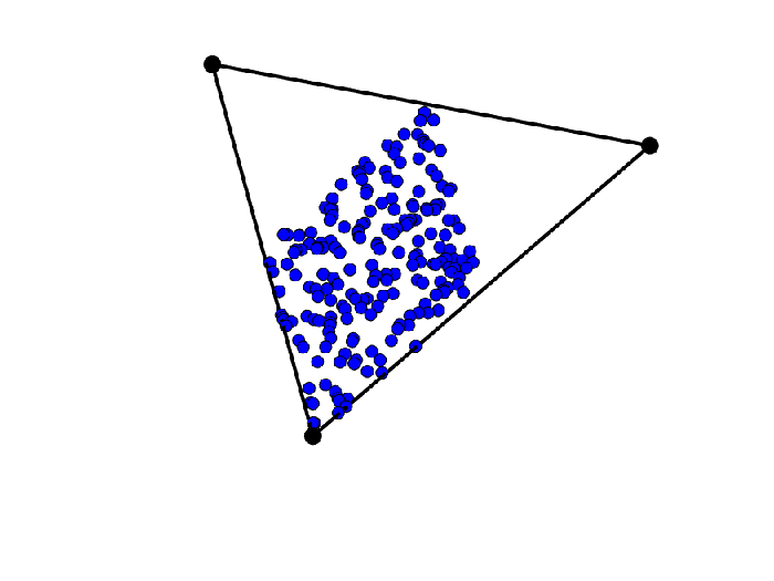
Refer to caption
(a) Vτ,1V_{\tau,1}
Refer to caption
(b) V∗,1V_{*,1}
Figure 1: Panel a: plot of Vτ,1V_{\tau,1} and the ideal simplex formed by Vτ,1(ℐ,:)V_{\tau,1}(\mathcal{I},:). Blue points denote mixed rows of Vτ,1V_{\tau,1}; Black points denote the KK rows of the corner matrix Vτ,1(ℐ,:)V_{\tau,1}(\mathcal{I},:) returned by SP algorithm (please refer to the supplementary material) when the input is Vτ,1V_{\tau,1}; Note that by Lemma 3.1, rows for pure nodes are same if these pure nodes are from the same cluster, hence rows for pure nodes coincide if these pure nodes are from the same cluster. Panel b: plot of V∗,1V_{*,1} and the hyperplane formed by V∗,1(ℐ,:)V_{*,1}(\mathcal{I},:). Blue points denote mixed rows of V∗,1V_{*,1}; Black points denote the KK rows of the corner matrix V∗,1(ℐ,:)V_{*,1}(\mathcal{I},:) returned by SVM-cone algorithm (please refer to the supplementary material) when the input is V∗,1V_{*,1}; We also plot the hyperplane formed by the triangle of the 3 rows of V∗,1(ℐ,:)V_{*,1}(\mathcal{I},:). Note that by Lemma 3.3, rows respective to pure nodes are same if these pure nodes are from the same cluster, hence rows refer to pure nodes from the same cluster coincide in ℝ3\mathbb{R}^{3} in this figure. For visualization, we have projected and rotated these points from ℝ3\mathbb{R}^{3} to ℝ2\mathbb{R}^{2}.

3.2 The Ideal Cone (IC) and the Ideal CRSC algorithm

In this subsection, we give another ideal algorithm.Actually, we normalize each rows of VV to have unit l2l_{2} length, then the newly obtained matrix has a structure called Ideal Cone (to be defined later). Then the SVM-cone algorithm (Mao et al. 2018) can be applied to hunt for the index set ℐ\mathcal{I}.

Let V∗,1V_{*,1} be the row-normalized version of VV such that V∗,1(i,:)=V(i,:)∥V(i,:)∥FV_{*,1}(i,:)=\frac{V(i,:)}{\|V(i,:)\|_{F}}. Let NVN_{V} be the n×nn\times n diagonal matrix such that NV(i,i)=1∥V(i,:)∥FN_{V}(i,i)=\frac{1}{\|V(i,:)\|_{F}} for 1≤i≤n1\leq i\leq n. Then V∗,1V_{*,1} can be rewritten as V∗,1=NV​VV_{*,1}=N_{V}V. Next lemma shows that each row of V∗,1V_{*,1} can be expressed by a scaled combination of V∗,1(ℐ,:)V_{*,1}(\mathcal{I},:). Combining it with the fact that each row of V∗,1V_{*,1} has unit l2l_{2} norm, the existence of the Ideal Cone is guaranteed.

Lemma 3.3.

Under M​M​S​B​(n,P,Π)MMSB(n,P,\Pi), there exists a Y1∈ℝ≥0n×KY_{1}\in\mathbb{R}^{n\times K}_{\geq 0} and no row of Y1Y_{1} is 0 such that

V∗,1=Y1V∗,1(ℐ,:),\displaystyle V_{*,1}=Y_{1}V_{*,1}(\mathcal{I},:),

where Y1Y_{1} can be written as Y1=NM1​Π​𝒟τ1/2​(ℐ,ℐ)​NV−1​(ℐ,ℐ)Y_{1}=N_{M_{1}}\Pi\mathscr{D}^{1/2}_{\tau}(\mathcal{I},\mathcal{I})N_{V}^{-1}(\mathcal{I},\mathcal{I}), where NM1N_{M_{1}} is an n×nn\times n diagonal matrix whose diagonal entries are positive. Meanwhile, for any two distinct nodes i,ji,j, when Π(i,:)=Π(j,:)\Pi(i,:)=\Pi(j,:), we have V∗,1(i,:)=V∗,1(j,:)V_{*,1}(i,:)=V_{*,1}(j,:).

Since rank⁡(V∗,1)=K\mathrm{rank}(V_{*,1})=K, rank(V∗,1(ℐ,:))=K\mathrm{rank}(V_{*,1}(\mathcal{I},:))=K. As V∗,1(ℐ,:)∈ℝK×KV_{*,1}(\mathcal{I},:)\in\mathbb{R}^{K\times K}, the inverse of V∗,1(ℐ,:)V_{*,1}(\mathcal{I},:) exists. Therefore, Lemma 3.3 also gives that

Y1=V∗,1V∗,1−1(ℐ,:).\displaystyle Y_{1}=V_{*,1}V^{-1}_{*,1}(\mathcal{I},:). (5)

Since V∗,1=NV​VV_{*,1}=N_{V}V and Y1=NM1​Π​𝒟τ1/2​(ℐ,ℐ)​NV−1​(ℐ,ℐ)Y_{1}=N_{M_{1}}\Pi\mathscr{D}^{1/2}_{\tau}(\mathcal{I},\mathcal{I})N_{V}^{-1}(\mathcal{I},\mathcal{I}), we have

NV−1NM1Π𝒟τ1/2(ℐ,ℐ)NV−1(ℐ,ℐ)=VV∗,1−1(ℐ,:),N_{V}^{-1}N_{M_{1}}\Pi\mathscr{D}^{1/2}_{\tau}(\mathcal{I},\mathcal{I})N_{V}^{-1}(\mathcal{I},\mathcal{I})=VV^{-1}_{*,1}(\mathcal{I},:),

i.e.,

NV−1NM1Π=VV∗,1−1(ℐ,:)NV(ℐ,ℐ)𝒟τ−1/2(ℐ,ℐ).\displaystyle N_{V}^{-1}N_{M_{1}}\Pi=VV^{-1}_{*,1}(\mathcal{I},:)N_{V}(\mathcal{I},\mathcal{I})\mathscr{D}^{-1/2}_{\tau}(\mathcal{I},\mathcal{I}). (6)

For convenience, set J∗,1=NV(ℐ,ℐ)𝒟τ−1/2(ℐ,ℐ),Z∗,1=NV−1NM1Π,Y∗,1=VV∗,1−1(ℐ,:)J_{*,1}=N_{V}(\mathcal{I},\mathcal{I})\mathscr{D}^{-1/2}_{\tau}(\mathcal{I},\mathcal{I}),Z_{*,1}=N_{V}^{-1}N_{M_{1}}\Pi,Y_{*,1}=VV^{-1}_{*,1}(\mathcal{I},:). By Eq (6), we have

Z∗,1=Y∗,1J∗,1≡VV∗,1−1(ℐ,:)NV(ℐ,ℐ)𝒟τ−1/2(ℐ,ℐ).\displaystyle Z_{*,1}=Y_{*,1}J_{*,1}\equiv VV^{-1}_{*,1}(\mathcal{I},:)N_{V}(\mathcal{I},\mathcal{I})\mathscr{D}^{-1/2}_{\tau}(\mathcal{I},\mathcal{I}). (7)

Meanwhile, since NV−1​NM1N_{V}^{-1}N_{M_{1}} is an n×nn\times n positive diagonal matrix, we have

Π(i,:)=Z∗,1(i,:)∥Z∗,1(i,:)∥1,1≤i≤n.\displaystyle\Pi(i,:)=\frac{Z_{*,1}(i,:)}{\|Z_{*,1}(i,:)\|_{1}},1\leq i\leq n. (8)

The above analysis shows that once the index set ℐ\mathcal{I} is known, we can exactly recover Π\Pi by Eq. (8).

Thus, the only difficulty is in finding the index set ℐ\mathcal{I}. From Lemma 3.3, we know that V∗,1=Y1V∗,1(ℐ,:)V_{*,1}=Y_{1}V_{*,1}(\mathcal{I},:) forms the Ideal Cone. The SVM-cone algorithm can be used to obtain the corner indices set ℐS​V​M−c​o​n​e\mathcal{I}_{SVM-cone} from the Ideal Cone. And the condition for using SVM-cone is satisfied, i.e., (V∗,1(ℐ,:)V∗,1′(ℐ,:))−1𝟏>0(V_{*,1}(\mathcal{I},:)V^{\prime}_{*,1}(\mathcal{I},:))^{-1}\mathbf{1}>0 holds (see Lemma 3.4). Though ℐS​V​M−c​o​n​e\mathcal{I}_{SVM-cone} may differ from ℐ\mathcal{I}, Π(ℐS​V​M−c​o​n​e(k),:)=Π(ℐ(k),:)\Pi(\mathcal{I}_{SVM-cone}(k),:)=\Pi(\mathcal{I}(k),:) for 1≤k≤K1\leq k\leq K, see the supplementary material. Hence, we also use ℐ\mathcal{I} to denote ℐS​V​M−c​o​n​e\mathcal{I}_{SVM-cone}.

Lemma 3.4.

Under D​C​M​M​(n,P,Θ,Π)DCMM(n,P,\Theta,\Pi), (V∗,1(ℐ,:)V∗,1′(ℐ,:))−1𝟏>0(V_{*,1}(\mathcal{I},:)V^{\prime}_{*,1}(\mathcal{I},:))^{-1}\mathbf{1}>0 holds.

From the above analysis we construct the following algorithm called Ideal Cone Regularized Spectral Clustering (Ideal CRSC for short). Input Ω,K\Omega,K. Output: Π\Pi.

  • •

    RSC step.

    • –

      Obtain 𝒟τ,ℒτ\mathscr{D}_{\tau},\mathscr{L}_{\tau}, VV, V∗,1V_{*,1} and NVN_{V}.

  • •

    Corners Hunting (CH) step.

    • –

      Run SVM-cone algorithm with inputs V∗,1V_{*,1} and KK to obtain the corner matrix V∗,1(ℐ,:)V_{*,1}(\mathcal{I},:).

  • •

    Membership Reconstruction (MR) step.

    • –

      Recover Y∗,1Y_{*,1} and J∗,1J_{*,1} by setting Y∗,1=VV∗,1−1(ℐ,:),J∗,1=NV(ℐ,ℐ)𝒟τ−1/2(ℐ,ℐ)Y_{*,1}=VV^{-1}_{*,1}(\mathcal{I},:),J_{*,1}=N_{V}(\mathcal{I},\mathcal{I})\mathscr{D}^{-1/2}_{\tau}(\mathcal{I},\mathcal{I}).

    • –

      Recover Z∗,1Z_{*,1} by setting Z∗,1=Y∗,1​J∗,1Z_{*,1}=Y_{*,1}J_{*,1}.

    • –

      Recover Π(i,:)\Pi(i,:) by setting Π(i,:)=Z∗,1(i,:)∥Z∗,1(i,:)∥1\Pi(i,:)=\frac{Z_{*,1}(i,:)}{\|Z_{*,1}(i,:)\|_{1}} for 1≤i≤n1\leq i\leq n.

To demonstrate that V∗,1V_{*,1} has the ideal cone structure, we drew panel (b) of Figure 1, where panel (b) is obtained under the same setting as panel (a) (i.e., after computing ℒτ\mathscr{L}_{\tau}, then obtain V∗,1V_{*,1}. Run SVM-cone algorithm on V∗,1V_{*,1} with K=3K=3 to obtain the index set ℐ\mathcal{I}, then we can plot panel (b) of Figure 1.). Panel (b) shows that all mixed rows of V∗,1V_{*,1} are located at one side of the hyperplane formed by the KK pure rows of V∗,1V_{*,1}. Meanwhile, the SVM-cone algorithm can exactly return the corner matrix V∗,1(ℐ,:)V_{*,1}(\mathcal{I},:) from V∗,1V_{*,1} with given KK, for detailed explanation of this statement, refer to the supplementary material.

3.3 The algorithms: SRSC and CRSC

We now extend the ideal case to the real case. The following two algorithms, which we call Simplex Regularized Spectral Clustering (SRSC for short) and Cone Regularized Spectral Clustering (CRSC for short) are natural extensions of the Ideal SRSC and the Ideal CRSC, respectively.

Algorithm 1 Simplex Regularized Spectral Clustering (SRSC for short)
1: The adjacency matrix A∈ℝn×nA\in\mathbb{R}^{n\times n}, the number of communities KK, and a ridge regularizer τ≥0\tau\geq 0.
2: The estimated n×Kn\times K membership matrix Π^1\hat{\Pi}_{1}.
3: RSC step.
  • •

    Obtain the graph Laplacian with ridge regularization by

    Lτ=Dτ−1/2ADτ−1/2,\displaystyle L_{\tau}=D_{\tau}^{-1/2}AD_{\tau}^{-1/2},

    where Dτ=D+τ​ID_{\tau}=D+\tau I, DD is an n×nn\times n diagonal matrix whose ii-th diagonal entry is D⁡(i,i)=∑j=1nA⁡(i,j)D(i,i)=\sum_{j=1}^{n}A(i,j) (unless specified, for SRSC, a good default τ\tau is τ=0.1​log​(n)\tau=0.1\mathrm{log}(n)).

  • •

    Let V^=[η^1,…,η^K]∈ℝn×K\hat{V}=[\hat{\eta}_{1},\ldots,\hat{\eta}_{K}]\in\mathbb{R}^{n\times K} denote the matrix containing the leading KK eigenvectors with unit-norm of LτL_{\tau}.

  • •

    Let V^τ,1=Dτ1/2​V^\hat{V}_{\tau,1}=D^{1/2}_{\tau}\hat{V}.

4: CH step.
  • •

    Apply SP algorithm on the rows of V^τ,1\hat{V}_{\tau,1} assuming there are KK clusters to obtain the near-corners matrix V^τ,1(ℐ^1,:)∈ℝK×K\hat{V}_{\tau,1}(\mathcal{\hat{I}}_{1},:)\in\mathbb{R}^{K\times K}, where ℐ^1\mathcal{\hat{I}}_{1} is the index set returned by SP algorithm.

5: Membership Reconstruction (MR) step.
  • •

    Estimate Z1Z_{1} by setting Z^1=V^V^τ,1−1(ℐ^1,:)\hat{Z}_{1}=\hat{V}\hat{V}^{-1}_{\tau,1}(\mathcal{\hat{I}}_{1},:).

  • •

    Set Z^1=max⁡(0,Z^1)\hat{Z}_{1}=\mathrm{max}(0,\hat{Z}_{1})

  • •

    Estimate Π(i,:)\Pi(i,:) by setting Π^1(i,:)=Z^1(i,:)/∥Z^1(i,:)∥1,1≤i≤n\hat{\Pi}_{1}(i,:)=\hat{Z}_{1}(i,:)/\|\hat{Z}_{1}(i,:)\|_{1},1\leq i\leq n.

Algorithm 2 Cone Regularized Spectral Clustering (CRSC for short)
1: The adjacency matrix A∈ℝn×nA\in\mathbb{R}^{n\times n}, the number of communities KK, and a ridge regularizer τ≥0\tau\geq 0.
2: The estimated n×Kn\times K membership matrix Π^∗,1\hat{\Pi}_{*,1}.
3: RSC step.
  • •

    Obtain Lτ,Dτ,V^L_{\tau},D_{\tau},\hat{V} as Algorithm 1 (unless specified, for CRSC, a good default τ\tau is τ=0.1​log​(n)\tau=0.1\mathrm{log}(n)). Let V^∗,1\hat{V}_{*,1} be the n×Kn\times K matrix such that V^∗,1(i,:)=V^(i,:)∥V^(i,:)∥F,i=1,2,…,n\hat{V}_{*,1}(i,:)=\frac{\hat{V}(i,:)}{\|\hat{V}(i,:)\|_{F}},i=1,2,\ldots,n. Obtain the n×nn\times n diagonal matrix NV^N_{\hat{V}}, whose ii-th diagonal entry is 1/∥V^(i,:)∥F1/\|\hat{V}(i,:)\|_{F}.

4: CH step.
  • •

    Apply SVM-cone algorithm on the rows of V^∗,1\hat{V}_{*,1} assuming there are KK clusters to obtain the estimated index set ℐ^∗,1\mathcal{\hat{I}}_{*,1}.

5: Membership Reconstruction (MR) step.
  • •

    Estimate Y∗,1Y_{*,1} by setting Y^∗,1=V^V^∗,1−1(ℐ^∗,1,:)\hat{Y}_{*,1}=\hat{V}\hat{V}^{-1}_{*,1}(\mathcal{\hat{I}}_{*,1},:).

  • •

    Estimate J∗,1J_{*,1} by setting J^∗,1=NV^(ℐ^∗,1,ℐ^∗,1)Dτ−1/2(ℐ^∗,1,ℐ^∗,1)\hat{J}_{*,1}=N_{\hat{V}}(\mathcal{\hat{I}}_{*,1},\mathcal{\hat{I}}_{*,1})D^{-1/2}_{\tau}(\mathcal{\hat{I}}_{*,1},\mathcal{\hat{I}}_{*,1}).

  • •

    Estimate Z∗,1Z_{*,1} by setting Z^∗,1=Y^∗,1​J^∗,1\hat{Z}_{*,1}=\hat{Y}_{*,1}\hat{J}_{*,1}.

  • •

    Set Z^∗,1=max⁡(0,Z^∗,1)\hat{Z}_{*,1}=\mathrm{max}(0,\hat{Z}_{*,1})

  • •

    Estimate Π(i,:)\Pi(i,:) by setting Π^∗,1(i,:)=Z^∗,1(i,:)/∥Z^∗,1(i,:)∥1,1≤i≤n\hat{\Pi}_{*,1}(i,:)=\hat{Z}_{*,1}(i,:)/\|\hat{Z}_{*,1}(i,:)\|_{1},1\leq i\leq n.

Remark 3.5.

Steps 1, 2, 3 in SRSC and CRSC are straightforward extensions of the three steps in the Ideal SRSC and the Ideal CRSC except that we set Z^1=max⁡(0,Z^1)\hat{Z}_{1}=\mathrm{max}(0,\hat{Z}_{1}) and Z^∗,1=max⁡(0,Z^∗,1)\hat{Z}_{*,1}=\mathrm{max}(0,\hat{Z}_{*,1}) to transform negative entries of Z^1,Z^∗,1\hat{Z}_{1},\hat{Z}_{*,1} into positive in the MR step due to the fact that V^V^τ−1(ℐ^1,:)\hat{V}\hat{V}^{-1}_{\tau}(\mathcal{\hat{I}}_{1},:) and Y^∗,1​J^∗,1\hat{Y}_{*,1}\hat{J}_{*,1} may contain a few negative entries in practice and we have to remore these negative entries since weights are nonnegative.

4 Equivalence algorithms

In this section, we design two algorithms SRSC-equivalence and CRSC-equivalence which give same estimations as Algorithms 1 and 2, respectively. We start this section by defining eight n×nn\times n matrices: V2,V^2,Vτ,2,V^τ,2,V∗,2,V^2,∗,NV2V_{2},\hat{V}_{2},V_{\tau,2},\hat{V}_{\tau,2},V_{*,2},\hat{V}_{2,*},N_{V_{2}} and NV^2N_{\hat{V}_{2}}.

Definition 4.1.

Set V2=V​V′,Vτ,2=𝒟τ1/2​V2,V^2=V^​V^′,V^τ,2=Dτ1/2​V^2V_{2}=VV^{\prime},V_{\tau,2}=\mathscr{D}^{1/2}_{\tau}V_{2},\hat{V}_{2}=\hat{V}\hat{V}^{\prime},\hat{V}_{\tau,2}=D^{1/2}_{\tau}\hat{V}_{2}. Set V∗,2,V^∗,2V_{*,2},\hat{V}_{*,2} such that V∗,2(i,:)=V2(i,:)∥V2(i,:)∥F,V^∗,2(i,:)=V^2(i,:)∥V^2(i,:)∥FV_{*,2}(i,:)=\frac{V_{2}(i,:)}{\|V_{2}(i,:)\|_{F}},\hat{V}_{*,2}(i,:)=\frac{\hat{V}_{2}(i,:)}{\|\hat{V}_{2}(i,:)\|_{F}} for 1≤i≤n1\leq i\leq n. Let NV2,NV^2N_{V_{2}},N_{\hat{V}_{2}} be n×nn\times n diagonal matrices whose ii-th diagonal entries are 1∥V2(i,:)∥F\frac{1}{\|V_{2}(i,:)\|_{F}} and 1∥V^2(i,:)∥F\frac{1}{\|\hat{V}_{2}(i,:)\|_{F}}, respectively.

In next subsections, we will give the two equivalences algorithms after providing the Ideal SRSC-equivalence algorithm and the Ideal CRSC-equivalence algorithm based on analyzing the properties of Vτ,2V_{\tau,2} and V∗,2V_{*,2}.

4.1 The SRSC-equivalence algorithm

To introduce the SRSC-equivalence algorithm, similar as the SRSC algorithm, we start from the ideal case. First we show that there exists the Ideal Simplex structure in Vτ,2V_{\tau,2} by Lemma 4.2.

Lemma 4.2.

Under M​M​S​B​(n,P,Π)MMSB(n,P,\Pi), we have Vτ,2=ΠVτ,2(ℐ,:)V_{\tau,2}=\Pi V_{\tau,2}(\mathcal{I},:). Meanwhile, for any two distinct nodes i,ji,j, we have Vτ,2(i,:)=Vτ,2(j,:)V_{\tau,2}(i,:)=V_{\tau,2}(j,:) when Π(i,:)=Π(j,:)\Pi(i,:)=\Pi(j,:).

Remark 4.3.

Similar as Remark 3.2, though the index set ℐ\mathcal{I} may be different, Vτ,2(ℐ,:)V_{\tau,2}(\mathcal{I},:) is always the same.

Since Vτ,2(ℐ,:)∈ℝK×nV_{\tau,2}(\mathcal{I},:)\in\mathbb{R}^{K\times n}, Vτ,2(ℐ,:)V_{\tau,2}(\mathcal{I},:) is a singular matrix. Based on conditions (I1) and (I2), Vτ,2(ℐ,:)Vτ,2′(ℐ,:)V_{\tau,2}(\mathcal{I},:)V^{\prime}_{\tau,2}(\mathcal{I},:) is non-singular. By Lemma 4.2, we have Π=Vτ,2Vτ,2′(ℐ,:)(Vτ,2(ℐ,:)Vτ,2′(ℐ,:))−1\Pi=V_{\tau,2}V^{\prime}_{\tau,2}(\mathcal{I},:)(V_{\tau,2}(\mathcal{I},:)V^{\prime}_{\tau,2}(\mathcal{I},:))^{-1}. Since Vτ,2=𝒟τ1/2​V2V_{\tau,2}=\mathscr{D}^{1/2}_{\tau}V_{2}, we have

Z2≡𝒟τ−1/2Π=V2Vτ,2′(ℐ,:)(Vτ,2(ℐ,:)Vτ,2′(ℐ,:))−1,\displaystyle Z_{2}\equiv\mathscr{D}^{-1/2}_{\tau}\Pi=V_{2}V^{\prime}_{\tau,2}(\mathcal{I},:)(V_{\tau,2}(\mathcal{I},:)V^{\prime}_{\tau,2}(\mathcal{I},:))^{-1}, (9)

where we set Z2=𝒟−1/2τΠZ_{2}=\mathscr{D}^{-1/2}_{\tau}\Pi for convenience. Then we have Π(i,:)=Z2(i,:)∥Z2(i,:)∥1\Pi(i,:)=\frac{Z_{2}(i,:)}{\|Z_{2}(i,:)\|_{1}}. Now, if we are given Ω\Omega and KK in advance but without known Π\Pi and PP, then we can compute ℒτ,V2\mathscr{L}_{\tau},V_{2} and Vτ,2V_{\tau,2}. According to Eq (9) and Remark 4.3, as long as we know the corner matrix Vτ,2(ℐ,:)V_{\tau,2}(\mathcal{I},:), we can obtain Π\Pi by normalizing each rows of Z2Z_{2} to have unit l1l_{1} norm. Thus, the only difficulty is in finding ℐ\mathcal{I}. Similar as the Ideal SRSC algorithm, due to the Ideal Simplex form Vτ,2=ΠVτ,2(ℐ,:)V_{\tau,2}=\Pi V_{\tau,2}(\mathcal{I},:), with given Vτ,2V_{\tau,2} and KK, SP algorithm can find the corner matrix Vτ,2(I,:)V_{\tau,2}(I,:).

The above analysis gives rise to the following three-stage algorithm which we call the Ideal SRSC-equivalence algorithm. Input Ω,K\Omega,K. Output: Π\Pi.

  • •

    RSC step.

    • –

      Obtain 𝒟τ=𝒟+τ​I\mathscr{D}_{\tau}=\mathscr{D}+\tau I, ℒτ\mathscr{L}_{\tau}, VV and Vτ,2V_{\tau,2}.

  • •

    Corners Hunting (CH) step.

    • –

      Run SP algorithm with inputs Vτ,2V_{\tau,2} to obtain Vτ,2(ℐ,:)V_{\tau,2}(\mathcal{I},:).

  • •

    Membership Reconstruction (MR) step.

    • –

      Recover Z2Z_{2} by setting Z2=V2Vτ,2′(ℐ,:)(Vτ,2(ℐ,:)Vτ,2′(ℐ,:))−1Z_{2}=V_{2}V^{\prime}_{\tau,2}(\mathcal{I},:)(V_{\tau,2}(\mathcal{I},:)V^{\prime}_{\tau,2}(\mathcal{I},:))^{-1}.

    • –

      Recover Π(i,:)\Pi(i,:) by setting Π(i,:)=Z2(i,:)∥Z2(i,:)∥1\Pi(i,:)=\frac{Z_{2}(i,:)}{\|Z_{2}(i,:)\|_{1}} for 1≤i≤n1\leq i\leq n.

The above analysis shows that the Ideal SRSC-equivalence exactly recovers the membership matrix Π\Pi. We now extend the ideal case to the real case as below.

Algorithm 3 SRSC-equivalence
1: The adjacency matrix A∈ℝn×nA\in\mathbb{R}^{n\times n}, the number of communities KK, and a ridge regularizer τ≥0\tau\geq 0.
2: The estimated n×Kn\times K membership matrix Π^2\hat{\Pi}_{2}.
3: RSC step.
  • •

    Obtain Dτ,Lτ,V^D_{\tau},L_{\tau},\hat{V} as Algorithm 1.

  • •

    Let V^2=V^​V^′\hat{V}_{2}=\hat{V}\hat{V}^{\prime} and V^τ,2=Dτ1/2​V^2\hat{V}_{\tau,2}=D^{1/2}_{\tau}\hat{V}_{2}.

4: CH step.
  • •

    Apply SP algorithm on the rows of V^τ,2\hat{V}_{\tau,2} assuming there are KK clusters to obtain the near-corners matrix V^τ,2(ℐ^2,:)∈ℝK×n\hat{V}_{\tau,2}(\mathcal{\hat{I}}_{2},:)\in\mathbb{R}^{K\times n}, where ℐ^2\mathcal{\hat{I}}_{2} is the index set returned by SP algorithm.

5: Membership Reconstruction (MR) step.
  • •

    Estimate Z2Z_{2} by setting Z^2=V^2V^τ,2′(ℐ^2,:)(V^τ,2(ℐ^2,:)V^τ,2′(ℐ^2,:))−1\hat{Z}_{2}=\hat{V}_{2}\hat{V}^{\prime}_{\tau,2}(\mathcal{\hat{I}}_{2},:)(\hat{V}_{\tau,2}(\mathcal{\hat{I}}_{2},:)\hat{V}^{\prime}_{\tau,2}(\mathcal{\hat{I}}_{2},:))^{-1}.

  • •

    Set Z^2=max⁡(0,Z^2)\hat{Z}_{2}=\mathrm{max}(0,\hat{Z}_{2})

  • •

    Estimate Π(i,:)\Pi(i,:) by setting Π^2(i,:)=Z^2(i,:)/∥Z^2(i,:)∥1,1≤i≤n\hat{\Pi}_{2}(i,:)=\hat{Z}_{2}(i,:)/\|\hat{Z}_{2}(i,:)\|_{1},1\leq i\leq n.

4.2 The CRSC-equivalence algorithm

In this subsection, we introduce the CRSC-equivalence algorithm by starting from the ideal case. Next lemma shows V∗,2V_{*,2} has the Ideal Cone structure similar as V∗,1V_{*,1}.

Lemma 4.4.

Under M​M​S​B​(n,P,Π)MMSB(n,P,\Pi), there exists a Y2∈ℝ≥0n×KY_{2}\in\mathbb{R}^{n\times K}_{\geq 0} and no row of Y2Y_{2} is 0 such that

V∗,2=Y2V∗,2(ℐ,:),\displaystyle V_{*,2}=Y_{2}V_{*,2}(\mathcal{I},:),

where Y2=NM2​Π​𝒟τ1/2​(ℐ,ℐ)​NV2−1​(ℐ,ℐ)Y_{2}=N_{M_{2}}\Pi\mathscr{D}^{1/2}_{\tau}(\mathcal{I},\mathcal{I})N_{V_{2}}^{-1}(\mathcal{I},\mathcal{I}), where NM2N_{M_{2}} is an n×nn\times n diagonal matrix whose diagonal entries are positive. Meanwhile, V∗,2(i,:)=V∗,2(j,:)V_{*,2}(i,:)=V_{*,2}(j,:) holds when Π(i,:)=Π(j,:)\Pi(i,:)=\Pi(j,:).

Since V∗,2(ℐ,:)∈ℝK×nV_{*,2}(\mathcal{I},:)\in\mathbb{R}^{K\times n}, V∗,2(ℐ,:)V_{*,2}(\mathcal{I},:) is singular but V∗,2(ℐ,:)V∗,2′(ℐ,:)V_{*,2}(\mathcal{I},:)V^{\prime}_{*,2}(\mathcal{I},:) is nonsingular, by Lemma 4.4, we have

Y2=V∗,2V∗,2′(ℐ,:)(V∗,2(ℐ,:)V∗,2′(ℐ,:))−1.\displaystyle Y_{2}=V_{*,2}V^{\prime}_{*,2}(\mathcal{I},:)(V_{*,2}(\mathcal{I},:)V^{\prime}_{*,2}(\mathcal{I},:))^{-1}. (10)

Since V∗,2=NV2​V2,Y2=NM2​Π​𝒟τ1/2​(ℐ,ℐ)​NV2−1​(ℐ,ℐ)V_{*,2}=N_{V_{2}}V_{2},Y_{2}=N_{M_{2}}\Pi\mathscr{D}^{1/2}_{\tau}(\mathcal{I},\mathcal{I})N_{V_{2}}^{-1}(\mathcal{I},\mathcal{I}), we have NV2−1NM2Π𝒟τ1/2(ℐ,ℐ)NV2−1(ℐ,ℐ)=V2V∗,2′(ℐ,:)(V∗,2(ℐ,:)V∗,2′(ℐ,:))−1N_{V_{2}}^{-1}N_{M_{2}}\Pi\mathscr{D}^{1/2}_{\tau}(\mathcal{I},\mathcal{I})N_{V_{2}}^{-1}(\mathcal{I},\mathcal{I})=V_{2}V^{\prime}_{*,2}(\mathcal{I},:)(V_{*,2}(\mathcal{I},:)V^{\prime}_{*,2}(\mathcal{I},:))^{-1}, which gives that

NV2−1NM2Π=V2V∗,2′(ℐ,:)(V∗,2(ℐ,:)V∗,2′(ℐ,:))−1NV2(ℐ,ℐ)𝒟τ−1/2(ℐ,ℐ).\displaystyle N_{V_{2}}^{-1}N_{M_{2}}\Pi=V_{2}V^{\prime}_{*,2}(\mathcal{I},:)(V_{*,2}(\mathcal{I},:)V^{\prime}_{*,2}(\mathcal{I},:))^{-1}N_{V_{2}}(\mathcal{I},\mathcal{I})\mathscr{D}^{-1/2}_{\tau}(\mathcal{I},\mathcal{I}). (11)

For convenience, set J∗,2=NV2(ℐ,ℐ)𝒟τ−1/2(ℐ,ℐ),Z∗,2=NV2−1NM2Π,Y∗,2=V2V∗,2′(ℐ,:)(V∗,2(ℐ,:)V∗,2′(ℐ,:))−1J_{*,2}=N_{V_{2}}(\mathcal{I},\mathcal{I})\mathscr{D}^{-1/2}_{\tau}(\mathcal{I},\mathcal{I}),Z_{*,2}=N_{V_{2}}^{-1}N_{M_{2}}\Pi,Y_{*,2}=V_{2}V^{\prime}_{*,2}(\mathcal{I},:)(V_{*,2}(\mathcal{I},:)V^{\prime}_{*,2}(\mathcal{I},:))^{-1}. By Eq (11), we have

Z∗,2=Y∗,2J∗,2≡V2V∗,2′(ℐ,:)(V∗,2(ℐ,:)V∗,2′(ℐ,:))−1NV2(ℐ,ℐ)𝒟τ−1/2(ℐ,ℐ).\displaystyle Z_{*,2}=Y_{*,2}J_{*,2}\equiv V_{2}V^{\prime}_{*,2}(\mathcal{I},:)(V_{*,2}(\mathcal{I},:)V^{\prime}_{*,2}(\mathcal{I},:))^{-1}N_{V_{2}}(\mathcal{I},\mathcal{I})\mathscr{D}^{-1/2}_{\tau}(\mathcal{I},\mathcal{I}). (12)

Meanwhile, since NV2−1​NM2N_{V_{2}}^{-1}N_{M_{2}} is an n×nn\times n positive diagonal matrix, we have Π(i,:)=Z∗,2(i,:)∥Z∗,2(i,:)∥1\Pi(i,:)=\frac{Z_{*,2}(i,:)}{\|Z_{*,2}(i,:)\|_{1}} for 1≤i≤n1\leq i\leq n. Then we have the following Ideal CRSC-equivalence algorithm. Input Ω,K\Omega,K. Output: Π\Pi.

  • •

    RSC step.

    • –

      Obtain 𝒟τ,ℒτ\mathscr{D}_{\tau},\mathscr{L}_{\tau}, VV, V2=V​V′V_{2}=VV^{\prime} and the row-normalization version of V2V_{2}, V∗,2V_{*,2}. Compute NV2N_{V_{2}}.

  • •

    Corners Hunting (CH) step

    • –

      Run SVM-cone algorithm with inputs V∗,2V_{*,2} and KK to obtain ℐ\mathcal{I}.

  • •

    Membership Reconstruction (MR) step.

    • –

      Recover Y∗,2Y_{*,2} and J∗,2J_{*,2} by setting Y∗,2=V2V∗,2′(ℐ,:)(V∗,2(ℐ,:)V∗,2′(ℐ,:))−1,J∗,2=NV2(ℐ,ℐ)𝒟τ−1/2(ℐ,ℐ)Y_{*,2}=V_{2}V^{\prime}_{*,2}(\mathcal{I},:)(V_{*,2}(\mathcal{I},:)V^{\prime}_{*,2}(\mathcal{I},:))^{-1},J_{*,2}=N_{V_{2}}(\mathcal{I},\mathcal{I})\mathscr{D}^{-1/2}_{\tau}(\mathcal{I},\mathcal{I}).

    • –

      Recover Z∗,2Z_{*,2} by setting Z∗,2=Y∗,2​J∗,2Z_{*,2}=Y_{*,2}J_{*,2}.

    • –

      Recover Π(i,:)\Pi(i,:) by setting Π(i,:)=Z∗,2(i,:)∥Z∗,2(i,:)∥1\Pi(i,:)=\frac{Z_{*,2}(i,:)}{\|Z_{*,2}(i,:)\|_{1}} for 1≤i≤n1\leq i\leq n.

We now extend the ideal case to the real case as below.

Algorithm 4 CRSC-equivalence
1: The adjacency matrix A∈ℝn×nA\in\mathbb{R}^{n\times n}, the number of communities KK, and a ridge regularizer τ≥0\tau\geq 0.
2: The estimated n×Kn\times K membership matrix Π^∗,2\hat{\Pi}_{*,2}.
3: RSC step.
  • •

    Obtain Lτ,Dτ,V^L_{\tau},D_{\tau},\hat{V} as Algorithm 1. Let V^2=V^​V^′\hat{V}_{2}=\hat{V}\hat{V}^{\prime}. Let V^∗,2\hat{V}_{*,2} be the n×nn\times n matrix such that V^∗,2(i,:)=V^2(i,:)∥V^2(i,:)∥F,i=1,2,…,n\hat{V}_{*,2}(i,:)=\frac{\hat{V}_{2}(i,:)}{\|\hat{V}_{2}(i,:)\|_{F}},i=1,2,\ldots,n. Obtain the n×nn\times n diagonal matrix NV^2N_{\hat{V}_{2}}, whose ii-th diagonal entry is 1/∥V^2(i,:)∥F1/\|\hat{V}_{2}(i,:)\|_{F}.

4: CH step.
  • •

    Apply SVM-cone algorithm on the rows of V^∗,2\hat{V}_{*,2} assuming there are KK clusters to obtain the estimated index set ℐ^∗,2\mathcal{\hat{I}}_{*,2}.

5: Membership Reconstruction (MR) step.
  • •

    Estimate Y∗,2Y_{*,2} by setting Y^∗,2=V^2V^∗,2′(ℐ^∗,2,:)(V^∗,2(ℐ^∗,2,:)V^∗,2′(ℐ^∗,2,:))−1\hat{Y}_{*,2}=\hat{V}_{2}\hat{V}^{\prime}_{*,2}(\mathcal{\hat{I}}_{*,2},:)(\hat{V}_{*,2}(\mathcal{\hat{I}}_{*,2},:)\hat{V}^{\prime}_{*,2}(\mathcal{\hat{I}}_{*,2},:))^{-1}.

  • •

    Estimate J∗,2J_{*,2} by setting J^∗,2=NV^2(ℐ^∗,2,ℐ^∗,2)Dτ−1/2(ℐ^∗,2,ℐ^∗,2)\hat{J}_{*,2}=N_{\hat{V}_{2}}(\mathcal{\hat{I}}_{*,2},\mathcal{\hat{I}}_{*,2})D^{-1/2}_{\tau}(\mathcal{\hat{I}}_{*,2},\mathcal{\hat{I}}_{*,2}).

  • •

    Estimate Z∗,2Z_{*,2} by setting Z^∗,2=Y^∗,2​J^∗,2\hat{Z}_{*,2}=\hat{Y}_{*,2}\hat{J}_{*,2}.

  • •

    Set Z^∗,2=max⁡(0,Z^∗,2)\hat{Z}_{*,2}=\mathrm{max}(0,\hat{Z}_{*,2})

  • •

    Estimate Π(i,:)\Pi(i,:) by setting Π^∗,2(i,:)=Z^∗,2(i,:)/∥Z^∗,2(i,:)∥1,1≤i≤n\hat{\Pi}_{*,2}(i,:)=\hat{Z}_{*,2}(i,:)/\|\hat{Z}_{*,2}(i,:)\|_{1},1\leq i\leq n.

4.3 The Equivalences

We now emphasize the equivalence of Algorithm 1 and Algorithm 3 as well as the equivalence of Algorithm 2 and Algorithm 4 by lemmas 4.5 and 4.6.

Lemma 4.5.

The SP algorithm will return the same node indices on both V^τ,1\hat{V}_{\tau,1} and V^τ,2\hat{V}_{\tau,2}. Meanwhile, the SVM-cone algorithm will return the same node indices on both V^∗,1\hat{V}_{*,1} and V^∗,2\hat{V}_{*,2}.

Lemma 4.6.

For the ideal case, under M​M​S​B​(n,P,Π)MMSB(n,P,\Pi), we have

  • •

    For Ideal SRSC and Ideal SRSC-equivalence, we have

    Vτ,2(ℐ:,)Vτ,2′(ℐ:,)≡Vτ,1(ℐ:,)Vτ,1′(ℐ:,),Z2≡Z1.\displaystyle V_{\tau,2}(\mathcal{I}:,)V^{\prime}_{\tau,2}(\mathcal{I}:,)\equiv V_{\tau,1}(\mathcal{I}:,)V^{\prime}_{\tau,1}(\mathcal{I}:,),Z_{2}\equiv Z_{1}.
  • •

    For Ideal CRSC and Ideal CRSC-equivalence, we have

    NV2≡NV,V∗,2(ℐ:,)V∗,2′(ℐ:,)≡V∗,1(ℐ:,)V∗,1′(ℐ:,),NM1≡NM2,\displaystyle N_{V_{2}}\equiv N_{V},V_{*,2}(\mathcal{I}:,)V^{\prime}_{*,2}(\mathcal{I}:,)\equiv V_{*,1}(\mathcal{I}:,)V^{\prime}_{*,1}(\mathcal{I}:,),N_{M_{1}}\equiv N_{M_{2}},
    Y2≡Y1,Y∗,2≡Y∗,1,J∗,2≡J∗,1,Z∗,2≡Z∗,1.\displaystyle Y_{2}\equiv Y_{1},Y_{*,2}\equiv Y_{*,1},J_{*,2}\equiv J_{*,1},Z_{*,2}\equiv Z_{*,1}.

For the empirical case, we have

  • •

    For SRSC and SRSC-equivalence, we have

    ℐ^2≡ℐ^1,V^τ,2(ℐ^2,:)V^τ,2′(ℐ^2,:)≡V^τ,1(ℐ^1,:)V^τ,1′(ℐ^1,:),Z^2≡Z^1,Π^2≡Π^1.\displaystyle\mathcal{\hat{I}}_{2}\equiv\mathcal{\hat{I}}_{1},\hat{V}_{\tau,2}(\mathcal{\hat{I}}_{2},:)\hat{V}^{\prime}_{\tau,2}(\mathcal{\hat{I}}_{2},:)\equiv\hat{V}_{\tau,1}(\mathcal{\hat{I}}_{1},:)\hat{V}^{\prime}_{\tau,1}(\mathcal{\hat{I}}_{1},:),\hat{Z}_{2}\equiv\hat{Z}_{1},\hat{\Pi}_{2}\equiv\hat{\Pi}_{1}.
  • •

    For CRSC and CRSC-equivalence, we have

    ℐ^∗,2≡ℐ^∗,1,V^∗,2(ℐ^∗,2,:)V^∗,2′(ℐ^∗,2,:)≡V^∗,1(ℐ^∗,1,:)V^∗,1′(ℐ^∗,1,:),\displaystyle\mathcal{\hat{I}}_{*,2}\equiv\mathcal{\hat{I}}_{*,1},\hat{V}_{*,2}(\mathcal{\hat{I}}_{*,2},:)\hat{V}^{\prime}_{*,2}(\mathcal{\hat{I}}_{*,2},:)\equiv\hat{V}_{*,1}(\mathcal{\hat{I}}_{*,1},:)\hat{V}^{\prime}_{*,1}(\mathcal{\hat{I}}_{*,1},:),
    Y^∗,2≡Y^∗,1,J^∗,2≡J^∗,1,Z^∗,2≡Z^∗,1,Π^∗,2≡Π^∗,1.\displaystyle\hat{Y}_{*,2}\equiv\hat{Y}_{*,1},\hat{J}_{*,2}\equiv\hat{J}_{*,1},\hat{Z}_{*,2}\equiv\hat{Z}_{*,1},\hat{\Pi}_{*,2}\equiv\hat{\Pi}_{*,1}.

Lemma 4.6 guarantees that Algorithm 1 and Algorithm 3 return same outputs. Lemma 4.6 also guarantees that Algorithm 2 and Algorithm 4 return same outputs.

After showing the equivalences, from now on, for notation convenience, set Z≡Z1,N≡NV,NM≡NM1,Y≡Y1,Y∗≡Y∗,1,J∗≡J∗,1,Z∗≡Z∗,1Z\equiv Z_{1},N\equiv N_{V},N_{M}\equiv N_{M_{1}},Y\equiv Y_{1},Y_{*}\equiv Y_{*,1},J_{*}\equiv J_{*,1},Z_{*}\equiv Z_{*,1}, and N^≡NV^2,ℐ^≡ℐ^1,Z^≡Z^1,Π^≡Π^1,ℐ^∗≡ℐ^∗,1,Y^∗≡Y^∗,1,J^∗≡J^∗,1,Z^∗≡Z^∗,1,Π^∗≡Π^∗,1\hat{N}\equiv N_{\hat{V}_{2}},\mathcal{\hat{I}}\equiv\mathcal{\hat{I}}_{1},\hat{Z}\equiv\hat{Z}_{1},\hat{\Pi}\equiv\hat{\Pi}_{1},\mathcal{\hat{I}}_{*}\equiv\mathcal{\hat{I}}_{*,1},\hat{Y}_{*}\equiv\hat{Y}_{*,1},\hat{J}_{*}\equiv\hat{J}_{*,1},\hat{Z}_{*}\equiv\hat{Z}_{*,1},\hat{\Pi}_{*}\equiv\hat{\Pi}_{*,1}.

5 Main Results

In this section, we establish the performance guarantees for SRSC and CRSC. Since both methods are designed based on regularized Laplacian matrix, we first study several theoretical properties of the population and sample regularized Laplacian matrix. First, we make the following assumption

  • (A1)

    For two positive numbers α\alpha and β\beta, ρ​nlog⁡(nα​K−β)​⟶n→∞​∞\frac{\rho n}{\mathrm{log}(n^{\alpha}K^{-\beta})}\overset{n\rightarrow\infty}{\longrightarrow}\infty.

Assumption (A1) means that the network can not be too sparse when nn is large. Meanwhile, when K=O⁡(1)K=O(1) or β=0\beta=0, assumption (A1) is equivalent to ρ​n\rho n should grow faster than log⁡(n)\mathrm{log}(n). In Lemma 5.2, we will show that α,β\alpha,\beta are directly related with the probability on the bound of ‖Lτ−ℒτ‖\|L_{\tau}-\mathscr{L}_{\tau}\| as well as the optimal choice of τ\tau in Theorem 5.9.

Remark 5.1.

In the language of Mao et al. 2020, its Assumption 3.1 requires |λK​(Ω)|≥4​ρ​n​logξ​(n)|\lambda_{K}(\Omega)|\geq 4\sqrt{\rho n}\mathrm{log}^{\xi}(n) for ξ>1\xi>1. Recall that |λK​(Ω)|≤‖Ω‖=ρ​‖Π′​P~​Π‖=O⁡(ρ​n)|\lambda_{K}(\Omega)|\leq\|\Omega\|=\rho\|\Pi^{\prime}\tilde{P}\Pi\|=O(\rho n), we have O⁡(ρ​n)≥|λK​(Ω)|≥4​ρ​n​logξ​(n)O(\rho n)\geq|\lambda_{K}(\Omega)|\geq 4\sqrt{\rho n}\mathrm{log}^{\xi}(n), which gives that ρ​n≥O⁡(log2​ξ​(n))\rho n\geq O(\mathrm{log}^{2\xi}(n)). Therefore, Mao et al. 2020’s Assumption 3.1 on ρ​n\rho n should be ρ​n≥O⁡(log2​ξ​(n))\rho n\geq O(\mathrm{log}^{2\xi}(n)) (this is consistent with their Theorem F.1.) for ξ>1\xi>1 instead of ρ​n=O⁡(log⁡(n))\rho n=O(\mathrm{log}(n)), and Table 1 in Lei 2019 also pointed out this. For comparison, when α=1,β=0\alpha=1,\beta=0, our requirement on ρ​n\rho n in Condition (A1) is ρ​n≥O⁡(logξ​(n))\rho n\geq O(\mathrm{log}^{\xi}(n)), which gives that based on the regularized Laplacian matrix LτL_{\tau}, our requirement on the sparsity parameter ρ\rho in Condition (A1) is weaker than the requirement of ρ\rho based on the adjacency matrix AA in Mao et al. 2020. This guarantees that our two methods designed based on regularized Laplacian matrix LτL_{\tau} can detect sparser networks than the SPACL algorithm (Mao et al. 2020) designed based on AA for mixed membership community detection under MMSB.

For convenience, set δmin=min1≤i≤n​𝒟​(i,i),δmax=max1≤i≤n​𝒟​(i,i)\delta_{\mathrm{min}}=\underset{1\leq i\leq n}{\mathrm{min}}\mathscr{D}(i,i),\delta_{\mathrm{max}}=\underset{1\leq i\leq n}{\mathrm{max}}\mathscr{D}(i,i).

Lemma 5.2.

Under M​M​S​B​(n,P,Π)MMSB(n,P,\Pi), suppose Condition (A1) holds, with probability at least 1−o⁡(K4​βn4​α−1)1-o(\frac{K^{4\beta}}{n^{4\alpha-1}}), we have

‖Lτ−ℒτ‖={O⁡(ρ​n​log​(nα​K−β)τ+δmin),when ​C​ρ​n​log​(nα​K−β)≤τ+δmin≤C​ρ​n,O⁡(ρ​n​log​(nα​K−β)(τ+δmin)2),when ​τ+δmin<C​ρ​n​log​(nα​K−β).\displaystyle\|L_{\tau}-\mathscr{L}_{\tau}\|=\begin{cases}O(\frac{\sqrt{\rho n\mathrm{log}(n^{\alpha}K^{-\beta})}}{\tau+\delta_{\mathrm{min}}}),&\mbox{when }C\sqrt{\rho n\mathrm{log}(n^{\alpha}K^{-\beta})}\leq\tau+\delta_{\mathrm{min}}\leq C\rho n,\\ O(\frac{\rho n\mathrm{log}(n^{\alpha}K^{-\beta})}{(\tau+\delta_{\mathrm{min}})^{2}}),&\mbox{when~}\tau+\delta_{\mathrm{min}}<C\sqrt{\rho n\mathrm{log}(n^{\alpha}K^{-\beta})}.\end{cases}
Remark 5.3.

In Lemma 5.2, we see that τ+δmin\tau+\delta_{\mathrm{min}} has a upper bound C​ρ​nC\rho n (hence, τ≤C​ρ​n\tau\leq C\rho n) for some C>0C>0 and τ\tau should be nonnegative since τ+δmin\tau+\delta_{\mathrm{min}} is in the denominator position in the bound. Therefore, even we set τ\tau as 0, the bound in Lemma 5.2 is also meaningful. The upper bound C​ρ​nC\rho n of τ+δmin\tau+\delta_{\mathrm{min}} occurs naturally in the proof of this lemma. Meanwhile, setting τ\tau to large is meaningless. By Lemma 4 in the supplementary material, we know that λ1=‖ℒτ‖≤δmaxτ+δmax\lambda_{1}=\|\mathscr{L}_{\tau}\|\leq\frac{\delta_{\mathrm{max}}}{\tau+\delta_{\mathrm{max}}}. Therefore, when τ\tau is too large (say, an extreme case that τ→∞\tau\rightarrow\infty), λ1\lambda_{1} tends to be zero, causing that ℒτ\mathscr{L}_{\tau} tends to be a zero matrix. And in this case, for any adjacency matrix AA whether it comes from MMSB or not, as long as D⁡(i,i)≠0D(i,i)\neq 0, LτL_{\tau} also tends to be a zero matrix, and ‖Lτ−ℒτ‖\|L_{\tau}-\mathscr{L}_{\tau}\| always tends to be zero when τ→∞\tau\rightarrow\infty. However, this is meaningless for community detection. Therefore, an appropriate upper bound for τ\tau is reasonable.

In Lemma 5.2, the convergence probability is related with parameter α\alpha and β\beta instead of a constant, and we call such probability as parametric probability. After giving the main result Theorem 5.9, we will provide an explanation on the convenience of the theoretically optimal choice of the regularizer τ\tau by the newly defined parametric probability. For convenience, denote e​r​rn=‖Lτ−ℒτ‖err_{n}=\|L_{\tau}-\mathscr{L}_{\tau}\|.

5.1 Performance guarantees for SRSC and CRSC

In this subsection, we aim to show the asymptotic consistency of SRSC and CRSC, i.e., to prove that Π^\hat{\Pi} and Π^∗\hat{\Pi}_{*} concentrate around Π\Pi if the sampled network is generated from the M​M​S​B​(n,P,Π)MMSB(n,P,\Pi). Meanwhile, to show the asymptotic property of these two methods, the three parameters K,P,ΠK,P,\Pi can change with nn. The theoretical error bounds given in Theorem 5.9 are directly related with the model parameters (n,P,Π)(n,P,\Pi) and KK, which allows the analyticity by changing these model parameters to see the influence of these parameters on SRSC and CRSC.

In Jin et al. 2017; Mao et al. 2018; Mao et al. 2020, main theoretical results for their proposed community detection methods hinge on a row-wise deviation bound for the eigenvectors of the adjacency matrix whether under MMSB or DCMM. Similarly, for our SRSC and CRSC, the main theoretical results (i.e., Theorem 5.9) also rely on the row-wise deviation bound for the eigenvector of the regularized Laplacian matrix. Different from the theoretical techniques in Theorem 3.1 in Mao et al. 2020 and Lemma C.3 in Jin et al. 2017, to obtain the row-wise deviation bound for the eigenvector of the regularized Laplacian matrix, we use a combination of Theorem 4.2.1 in Chen et al. 2020 and Lemma 5.1 in Lei et al. 2015.

Lemma 5.4.

(Row-wise eigenvector error) Under M​M​S​B​(n,P,Π)MMSB(n,P,\Pi), suppose Condition (A1) holds, assume |λK|≥C​ρ​n​log​(n)τ+δmin|\lambda_{K}|\geq C\frac{\sqrt{\rho n\mathrm{log}(n)}}{\tau+\delta_{\mathrm{min}}}, with probability at least 1−o⁡(K4​βn4​α−1)1-o(\frac{K^{4\beta}}{n^{4\alpha-1}}), we have

‖V^​V^′−V​V′‖2→∞=O⁡((τ+δmax)​K​log​(nα​K−β)(τ+δmin)​|λK​(P~)|​λK​(Π′​Π)​ρ).\displaystyle\|\hat{V}\hat{V}^{\prime}-VV^{\prime}\|_{2\rightarrow\infty}=O(\frac{(\tau+\delta_{\mathrm{max}})\sqrt{K\mathrm{log}(n^{\alpha}K^{-\beta})}}{(\tau+\delta_{\mathrm{min}})|\lambda_{K}(\tilde{P})|\lambda_{K}(\Pi^{\prime}\Pi)\sqrt{\rho}}).

For convenience, we set ϖ=‖V^​V^′−V​V′‖2→∞\varpi=\|\hat{V}\hat{V}^{\prime}-VV^{\prime}\|_{2\rightarrow\infty}. We will use the row-wise eigenvector error ϖ\varpi to construct the error bounds for our theoretical analysis for SRSC and CRSC. We emphasize that the statement of Lemma 5.4 considers both positive and negative eigenvalues of ℒτ\mathscr{L}_{\tau} and LτL_{\tau}.

Remark 5.5.

If one set the Θ\Theta in Jin et al. 2017 as Θ=ρ​I\Theta=\sqrt{\rho}I, we can see that the DCMM model degenerates to the M​M​S​B​(n,P,Π)MMSB(n,P,\Pi) considered in this paper. In this case, the row-wise eigenvector deviation in the 4th bullet of Lemma 2.1 in Jin et al. 2017 is O⁡(1|λK​(P~)|​K1.5n​log⁡(n)ρ​n)O(\frac{1}{|\lambda_{K}(\tilde{P})|}\frac{K^{1.5}}{\sqrt{n}}\sqrt{\frac{\mathrm{log}(n)}{\rho n}}) under their Conditions (where their conditions are our Condition (A1) and the assumption λK​(Π′​Π)=O⁡(nK)\lambda_{K}(\Pi^{\prime}\Pi)=O(\frac{n}{K}) when Θ=ρ​I\Theta=\sqrt{\rho}I), which is consistent with our bound in Lemma 5.4.

Based on the conditions in Lemma 5.4, we can obtain the choice of τ\tau through the following analysis. Since we assume that |λK|≥C​ρ​n​log​(n)τ+δmin|\lambda_{K}|\geq C\frac{\sqrt{\rho n\mathrm{log}(n)}}{\tau+\delta_{\mathrm{min}}}, combine with the fact that e​r​rn=C​ρ​n​log​(nα​K−β)τ+δminerr_{n}=C\frac{\sqrt{\rho n\mathrm{log}(n^{\alpha}K^{-\beta})}}{\tau+\delta_{\mathrm{min}}} when C​ρ​n​log​(nα​K−β)≤τ+δmin≤C​ρ​nC\sqrt{\rho n\mathrm{log}(n^{\alpha}K^{-\beta})}\leq\tau+\delta_{\mathrm{min}}\leq C\rho n, we have |λK|≥C​e​r​rn|\lambda_{K}|\geq Cerr_{n}. Due to the fact that |λK|≤λ1≤1|\lambda_{K}|\leq\lambda_{1}\leq 1 (by Lemma 4 in the supplementary material), we have e​r​rn≤1Cerr_{n}\leq\frac{1}{C}. On the one hand, when C​ρ​n​log​(nα​K−β)≤τ+δmin≤C​ρ​nC\sqrt{\rho n\mathrm{log}(n^{\alpha}K^{-\beta})}\leq\tau+\delta_{\mathrm{min}}\leq C\rho n, we have e​r​rn=O⁡(ρ​n​log​(nα​K−β)τ+δmin)err_{n}=O(\frac{\sqrt{\rho n\mathrm{log}(n^{\alpha}K^{-\beta})}}{\tau+\delta_{\mathrm{min}}}). By e​r​rn≤1/Cerr_{n}\leq 1/C, we see that τ+δmin≥C​ρ​n​log​(nα​K−β)\tau+\delta_{\mathrm{min}}\geq C\sqrt{\rho n\mathrm{log}(n^{\alpha}K^{-\beta})} by ignoring the effect of δmin\delta_{\mathrm{min}}, which is consistent with the case that τ+δmin≥C​ρ​n​log​(nα​K−β)\tau+\delta_{\mathrm{min}}\geq C\sqrt{\rho n\mathrm{log}(n^{\alpha}K^{-\beta})}. On the other hand, when τ+δmin<C​ρ​n​log​(nα​K−β)\tau+\delta_{\mathrm{min}}<C\sqrt{\rho n\mathrm{log}(n^{\alpha}K^{-\beta})}, we have e​r​rn=O⁡(ρ​n​log​(nα​K−β)(τ+δmin)2)err_{n}=O(\frac{\rho n\mathrm{log}(n^{\alpha}K^{-\beta})}{(\tau+\delta_{\mathrm{min}})^{2}}). As e​r​rn≤1/Cerr_{n}\leq 1/C, we see that τ+δmin≥C​ρ​n​log​(nα​K−β)\tau+\delta_{\mathrm{min}}\geq\sqrt{C\rho n\mathrm{log}(n^{\alpha}K^{-\beta})}, which is a contradiction. Hence, to make the condition of the lower bound of |λK||\lambda_{K}| hold, we need C​ρ​n​log​(nα​K−β)≤τ+δmin≤C​ρ​nC\sqrt{\rho n\mathrm{log}(n^{\alpha}K^{-\beta})}\leq\tau+\delta_{\mathrm{min}}\leq C\rho n, then e​r​rnerr_{n} can be always written as e​r​rn=O⁡(ρ​n​log​(nα​K−β)τ+δmin)err_{n}=O(\frac{\sqrt{\rho n\mathrm{log}(n^{\alpha}K^{-\beta})}}{\tau+\delta_{\mathrm{min}}}) under Condition (A1). Furthermore, from the requirement C​ρ​n​log​(nα​K−β)≤τ+δmin≤C​ρ​nC\sqrt{\rho n\mathrm{log}(n^{\alpha}K^{-\beta})}\leq\tau+\delta_{\mathrm{min}}\leq C\rho n, we can see that the benefit of regularization is that regularized spectral clustering (i.e., when τ>0\tau>0) can detect sparser networks than spectral clustering when τ=0\tau=0 due to the fact that if we set τ=0\tau=0, the lower bound requirement of δmin\delta_{\mathrm{min}} is C​ρ​n​log​(nα​K−β)C\sqrt{\rho n\mathrm{log}(n^{\alpha}K^{-\beta})}, which is larger than C​ρ​n​log​(nα​K−β)−τC\sqrt{\rho n\mathrm{log}(n^{\alpha}K^{-\beta})}-\tau when τ>0\tau>0. And such benefit can also be found in the main theorem 5.9 of this paper.

Bounds provided by Lemma 5.6 are the corner stones to characterize the behaviors of our SRSC and CRSC approaches. For convenience, set πmin=min1≤k≤K​𝟏′​Π​ek\pi_{\mathrm{min}}=\mathrm{min}_{1\leq k\leq K}\mathbf{1}^{\prime}\Pi e_{k}, where πmin\pi_{\mathrm{min}} measure the minimum summation of nodes belong to certain community and increasing πmin\pi_{\mathrm{min}} makes the network tend to be more balanced. For convenience, set η=min1≤k≤K((V∗,1(ℐ,:)V∗,1′(ℐ,:))−1𝟏)(k)\eta=\mathrm{min}_{1\leq k\leq K}((V_{*,1}(\mathcal{I},:)V^{\prime}_{*,1}(\mathcal{I},:))^{-1}\mathbf{1})(k).

Lemma 5.6.

Under M​M​S​B​(n,P,Π)MMSB(n,P,\Pi), when conditions of Lemma 5.4 hold, there exist two permutation matrices 𝒫,𝒫∗∈ℝK×K\mathcal{P},\mathcal{P}_{*}\in\mathbb{R}^{K\times K} such that with probability at least 1−o⁡(K4​βn4​α−1)1-o(\frac{K^{4\beta}}{n^{4\alpha-1}}), we have

∥V^τ,2(ℐ^,:)−𝒫Vτ,2(ℐ,:)∥F=O((τ+δmax)1.5​K​ϖ​κ​(Π′​Π)τ+δmin),\displaystyle\|\hat{V}_{\tau,2}(\mathcal{\hat{I}},:)-\mathcal{P}V_{\tau,2}(\mathcal{I},:)\|_{F}=O(\frac{(\tau+\delta_{\mathrm{max}})^{1.5}\sqrt{K}\varpi\kappa(\Pi^{\prime}\Pi)}{\tau+\delta_{\mathrm{min}}}),
∥V^∗,2(ℐ^∗,:)−𝒫∗V∗,2(ℐ,:)∥F=O((τ+δmaxτ+δmin)3.5K2.5​ϖ​κ3​(Π′​Π)​λ1​(Π′​Π)η).\displaystyle\|\hat{V}_{*,2}(\mathcal{\hat{I}}_{*},:)-\mathcal{P}_{*}V_{*,2}(\mathcal{I},:)\|_{F}=O((\frac{\tau+\delta_{\mathrm{max}}}{\tau+\delta_{\mathrm{min}}})^{3.5}\frac{K^{2.5}\varpi\kappa^{3}(\Pi^{\prime}\Pi)\sqrt{\lambda_{1}(\Pi^{\prime}\Pi)}}{\eta}).

Set ϖS=∥V^τ,2(ℐ^,:)−𝒫Vτ,2(ℐ,:)∥F,ϖC=∥V^∗,2(ℐ^,:)−𝒫∗V∗,2(ℐ,:)∥F\varpi_{S}=\|\hat{V}_{\tau,2}(\mathcal{\hat{I}},:)-\mathcal{P}V_{\tau,2}(\mathcal{I},:)\|_{F},\varpi_{C}=\|\hat{V}_{*,2}(\mathcal{\hat{I}},:)-\mathcal{P}_{*}V_{*,2}(\mathcal{I},:)\|_{F} for convenience in the proofs. Next lemma bounds the row-wise deviation between Y^∗\hat{Y}_{*} and Y∗Y_{*} for CRSC.

Lemma 5.7.

Under M​M​S​B​(n,P,Π)MMSB(n,P,\Pi), when conditions of Lemma 5.4 hold, with probability at least 1−o⁡(K4​βn4​α−1)1-o(\frac{K^{4\beta}}{n^{4\alpha-1}}), we have

max1≤i≤n​‖ei′​(Y^∗−Y∗​𝒫∗)‖F=O⁡((τ+δmaxτ+δmin)5​K3.5​ϖ​κ4.5​(Π′​Π)η).\displaystyle\mathrm{max}_{1\leq i\leq n}\|e^{\prime}_{i}(\hat{Y}_{*}-Y_{*}\mathcal{P}_{*})\|_{F}=O((\frac{\tau+\delta_{\mathrm{max}}}{\tau+\delta_{\mathrm{min}}})^{5}\frac{K^{3.5}\varpi\kappa^{4.5}(\Pi^{\prime}\Pi)}{\eta}).

Now we are ready to bound ‖ei′​(Z^−Z​𝒫)‖F\|e^{\prime}_{i}(\hat{Z}-Z\mathcal{P})\|_{F} and ‖ei′​(Z^∗−Z∗​𝒫∗)‖F\|e^{\prime}_{i}(\hat{Z}_{*}-Z_{*}\mathcal{P}_{*})\|_{F} based on Lemma 5.7.

Lemma 5.8.

Under M​M​S​B​(n,P,Π)MMSB(n,P,\Pi), when conditions of Lemma 5.4 hold, with probability at least 1−o⁡(K4​βn4​α−1)1-o(\frac{K^{4\beta}}{n^{4\alpha-1}}), we have

max1≤i≤n​‖ei′​(Z^−Z​𝒫)‖F=O⁡((τ+δmax)1.5​K​ϖ​κ​(Π′​Π)​λ1​(Π′​Π)(τ+δmin)2),\displaystyle\mathrm{max}_{1\leq i\leq n}\|e^{\prime}_{i}(\hat{Z}-Z\mathcal{P})\|_{F}=O(\frac{(\tau+\delta_{\mathrm{max}})^{1.5}K\varpi\kappa(\Pi^{\prime}\Pi)\sqrt{\lambda_{1}(\Pi^{\prime}\Pi)}}{(\tau+\delta_{\mathrm{min}})^{2}}),
max1≤i≤n​‖ei′​(Z^∗−Z∗​𝒫∗)‖F=O⁡((τ+δmax)7.5​K5.5​ϖ​κ4.5​(Π′​Π)​λ11.5​(Π′​Π)(τ+δmin)8​πmin).\displaystyle\mathrm{max}_{1\leq i\leq n}\|e^{\prime}_{i}(\hat{Z}_{*}-Z_{*}\mathcal{P}_{*})\|_{F}=O(\frac{(\tau+\delta_{\mathrm{max}})^{7.5}K^{5.5}\varpi\kappa^{4.5}(\Pi^{\prime}\Pi)\lambda^{1.5}_{1}(\Pi^{\prime}\Pi)}{(\tau+\delta_{\mathrm{min}})^{8}\pi_{\mathrm{min}}}).

Next theory is the main result for SRSC and CRSC to infer the membership parameters under MMSB.

Theorem 5.9.

Under M​M​S​B​(n,P,Π)MMSB(n,P,\Pi), when conditions of Lemma 5.4 hold, with probability at least 1−o⁡(K4​βn4​α−1)1-o(\frac{K^{4\beta}}{n^{4\alpha-1}}),

‖ei′​(Π^−Π​𝒫)‖F=O⁡((τ+δmax)3​K2​κ​(Π′​Π)​λ1​(Π′​Π)​log​(nα​K−β)(τ+δmin)3​|λK​(P~)|​λK​(Π′​Π)​ρ),\displaystyle\|e^{\prime}_{i}(\hat{\Pi}-\Pi\mathcal{P})\|_{F}=O(\frac{(\tau+\delta_{\mathrm{max}})^{3}K^{2}\kappa(\Pi^{\prime}\Pi)\sqrt{\lambda_{1}(\Pi^{\prime}\Pi)\mathrm{log}(n^{\alpha}K^{-\beta})}}{(\tau+\delta_{\mathrm{min}})^{3}|\lambda_{K}(\tilde{P})|\lambda_{K}(\Pi^{\prime}\Pi)\sqrt{\rho}}),
‖ei′​(Π^∗−Π​𝒫∗)‖F=O⁡((τ+δmax)9​K6.6​κ4.5​(Π′​Π)​λ11.5​(Π′​Π)​log⁡(nα​K−β)(τ+δmin)9​|λK​(P~)|​λK​(Π′​Π)​πmin​ρ).\displaystyle\|e^{\prime}_{i}(\hat{\Pi}_{*}-\Pi\mathcal{P}_{*})\|_{F}=O(\frac{(\tau+\delta_{\mathrm{max}})^{9}K^{6.6}\kappa^{4.5}(\Pi^{\prime}\Pi)\lambda^{1.5}_{1}(\Pi^{\prime}\Pi)\sqrt{\mathrm{log}(n^{\alpha}K^{-\beta})}}{(\tau+\delta_{\mathrm{min}})^{9}|\lambda_{K}(\tilde{P})|\lambda_{K}(\Pi^{\prime}\Pi)\pi_{\mathrm{min}}\sqrt{\rho}}).

Note that, when α=1,β=0\alpha=1,\beta=0, the convergence probability is 1−o⁡(n−3)1-o(n^{-3}), which is a common probability in community detection, see Jin 2015; Jin et al. 2017. For a general comparison of SRSC and CRSC, from Theorem 5.9, we see that CRSC is more sensitive on KK, κ⁡(Π′​Π)\kappa(\Pi^{\prime}\Pi) and unbalanced network (A larger τ+δmaxτ+δmin\frac{\tau+\delta_{\mathrm{max}}}{\tau+\delta_{\mathrm{min}}} refers to a more unbalanced network.) than SRSC. Both two methods have same sensitivity on the row-wise eigenvector deviation term ϖ\varpi. Generally, Theorem 5.9 says that the error bound for SRSC is slightly smaller than that of CRSC. Furthermore, Theorem 5.9 also says that a smaller β\beta and a larger α\alpha lead to a lager probability of successfully detecting mixed membership networks under MMSB. However, by Condition (A1), we see that smaller β\beta and larger α\alpha lead to stronger assumptions on the sparsity of a network under MMSB. Therefore, there is a trade-off between the sparsity of a network and the probability of successfully detecting its mixed memberships.

For both two methods, since δmin≤δmax\delta_{\mathrm{min}}\leq\delta_{\mathrm{max}}, when τ\tau increases, error bounds in Theorem 5.9 decrease, which suggests that a larger τ\tau gives better estimations. Recall that C​ρ​n​log​(nα​K−β)≤τ+δmin≤C​ρ​nC\sqrt{\rho n\mathrm{log}(n^{\alpha}K^{-\beta})}\leq\tau+\delta_{\mathrm{min}}\leq C\rho n, therefore the theoretical optimal choice of τ\tau is:

τopt=O⁡(ρ​n).\displaystyle\tau_{\mathrm{opt}}=O(\rho n). (13)

If we further add conditions similar as Corollary 3.1 in Mao et al. 2020, then we have the following corollary.

Corollary 5.10.

Under M​M​S​B​(n,P,Π)MMSB(n,P,\Pi), when conditions of Lemma 5.4 hold, set τ\tau as in Eq (13), suppose K=O⁡(1),πmin=O⁡(nK),λ1​(Π′​Π)=O⁡(nK)K=O(1),\pi_{\mathrm{min}}=O(\frac{n}{K}),\lambda_{1}(\Pi^{\prime}\Pi)=O(\frac{n}{K}), and δmax≤C​δmin\delta_{\mathrm{max}}\leq C\delta_{\mathrm{min}}, with probability at least 1−o⁡(K4​βn4​α−1)1-o(\frac{K^{4\beta}}{n^{4\alpha-1}}), we have

‖ei′​(Π^−Π​𝒫)‖F=O⁡(1|λK​(P~)|​log⁡(n)ρ​n),‖ei′​(Π^∗−Π​𝒫∗)‖F=O⁡(1|λK​(P~)|​log⁡(n)ρ​n).\displaystyle\|e^{\prime}_{i}(\hat{\Pi}-\Pi\mathcal{P})\|_{F}=O(\frac{1}{|\lambda_{K}(\tilde{P})|}\sqrt{\frac{\mathrm{log}(n)}{\rho n}}),~~~\|e^{\prime}_{i}(\hat{\Pi}_{*}-\Pi\mathcal{P}_{*})\|_{F}=O(\frac{1}{|\lambda_{K}(\tilde{P})|}\sqrt{\frac{\mathrm{log}(n)}{\rho n}}).

Especially, for the sparest case when ρ​n=O⁡(log1+2​ς​(n))\rho n=O(\mathrm{log}^{1+2\varsigma}(n)) for ς→0+\varsigma\rightarrow 0^{+}, we have

‖ei′​(Π^−Π​𝒫)‖F=O⁡(1|λK​(P~)|​logς​(n)),‖ei′​(Π^∗−Π​𝒫∗)‖F=O⁡(1|λK​(P~)|​logς​(n)).\displaystyle\|e^{\prime}_{i}(\hat{\Pi}-\Pi\mathcal{P})\|_{F}=O(\frac{1}{|\lambda_{K}(\tilde{P})|\mathrm{log}^{\varsigma}(n)}),~~~\|e^{\prime}_{i}(\hat{\Pi}_{*}-\Pi\mathcal{P}_{*})\|_{F}=O(\frac{1}{|\lambda_{K}(\tilde{P})|\mathrm{log}^{\varsigma}(n)}).
Remark 5.11.

Under the setting of Corollary 5.10, the condition |λK|≥C​ρ​n​log​(n)/(τ+δmin)|\lambda_{K}|\geq C\sqrt{\rho n\mathrm{log}(n)}/(\tau+\delta_{\mathrm{min}}) holds naturally. By Lemma 4 in the supplementary material, we know that |λK|≥ρ​|λK​(P~)​λK​(Π′​Π)|τ+δmax=C​ρ​|λK​(P~)|​nK⁡(τ+δmin)=C​ρ​n​|λK​(P~)|τ+δmin|\lambda_{K}|\geq\frac{\rho|\lambda_{K}(\tilde{P})\lambda_{K}(\Pi^{\prime}\Pi)|}{\tau+\delta_{\mathrm{max}}}=C\frac{\rho|\lambda_{K}(\tilde{P})|n}{K(\tau+\delta_{\mathrm{min}})}=C\frac{\rho n|\lambda_{K}(\tilde{P})|}{\tau+\delta_{\mathrm{min}}}. The inequality C​ρ​n​|λK​(P~)|τ+δmin≥C​ρ​n​log​(n)/(τ+δmin)C\frac{\rho n|\lambda_{K}(\tilde{P})|}{\tau+\delta_{\mathrm{min}}}\geq C\sqrt{\rho n\mathrm{log}(n)}/(\tau+\delta_{\mathrm{min}}) equals to |λK​(P~)|≥C​log⁡(n)ρ​n|\lambda_{K}(\tilde{P})|\geq C\sqrt{\frac{\mathrm{log}(n)}{\rho n}}, and it just matches with the requirement of the consistency of clustering in Corollary 5.10.

From Corollary 5.10, we see that when α\alpha is fixed, though a large β\beta lowers the requirement on the network sparsity in Condition (A1) (i.e., a large β\beta decreases the requirement on the lower bound on ρ​n\rho n), it decreases the probability (i.e., increasing β\beta decreases 1−o⁡(K4​βn4​α−1)1-o(\frac{K^{4\beta}}{n^{4\alpha-1}})). Similarly, when β\beta is fixed, though a small α\alpha lowers the requirement on the network sparsity in Condition (A1) (i.e., a decreasing α\alpha decreases the requirement on the lower bound on ρ​n\rho n), it decreases the probability (i.e., a decreasing α\alpha decreases 1−o⁡(K4​βn4​α−1)1-o(\frac{K^{4\beta}}{n^{4\alpha-1}})). When dealing with empirical networks, since α,β,ρ\alpha,\beta,\rho are unknown (i.e., we have no knowledge about the sparsity of the empirical networks), if τ\tau is too large (which can be seen as setting β\beta too large or α\alpha too small in Eq (13)), SRSC and CRSC can still work but with small convergence probability due to the fact that a very large β\beta or a very small α\alpha in Eq (13) decrease 1−o⁡(K4​βn4​α−1)1-o(\frac{K^{4\beta}}{n^{4\alpha-1}}). This explains that when dealing with empirical networks, even if τ\tau is very large, our methods still work but with small probability to have satisfactory performances, which suggesting that a moderate choice of τ\tau is preferred for both SRSC and CRSC. Meanwhile, as the statement after Theorem 5.9, τ\tau can not be too small.

Remark 5.12.

(Empirical optimal choice of τ\tau) Set α=1,β=0\alpha=1,\beta=0, then the convergence probabilities in the above lemmas, theorems and corollaries are 1−o⁡(n−3)1-o(n^{-3}). By (Eq 13), we see that τoptimal\tau_{\mathrm{optimal}} depends on ρ\rho where the parameter ρ\rho controls the sparsity of a network generated under M​M​S​B​(n,P,Π)MMSB(n,P,\Pi). Since most real world networks are sparse and K≪nK\ll n (i.e., KK can be seen as O⁡(1)O(1)), and network generated under the case that ρ​n=O⁡(log1+2​ς​(n))\rho n=O(\mathrm{log}^{1+2\varsigma}(n)) for any ς→0+\varsigma\rightarrow 0^{+} is the sparsest network satisfying Condition (A1), for such sparse network, by Eq (13) we should set τ\tau as τopt=O⁡(ρ​n)≡O⁡(log⁡(n))\tau_{\mathrm{opt}}=O(\rho n)\equiv O(\mathrm{log}(n)), where we set ς=0\varsigma=0 directly. Therefore, for both SRSC and CRSC, the optimal choices for τ\tau for the sparsest network satisfying Condition (A1) are the same, and we should set the optimal choice of τ\tau as

τopt=O⁡(log⁡(n)).\displaystyle\tau_{\mathrm{opt}}=O(\mathrm{log}(n)). (14)

Consider the balanced mixed membership network in Corollary 5.10, we further assume that P~=γ​IK+(1−γ)​IK​IK′\tilde{P}=\gamma I_{K}+(1-\gamma)I_{K}I^{\prime}_{K} for 0<γ<10<\gamma<1 when K=O⁡(1)K=O(1) and call such network as standard mixed membership network with KK balanced clusters. To obtain consistency estimation, γ\gamma should grow faster than log⁡(n)ρ​n\sqrt{\frac{\mathrm{log}(n)}{\rho n}} since |λK​(P)|=γ|\lambda_{K}(P)|=\gamma. Let Pmax=maxk,l⁡P⁡(k,l),Pmin=mink,l​P​(k,l)P_{\mathrm{max}}=\max_{k,l}P(k,l),P_{\mathrm{min}}=\mathrm{min}_{k,l}P(k,l). Consider the sparest case when ρ=O⁡(log1+2​ς​(n)n)\rho=O(\frac{\mathrm{log}^{1+2\varsigma}(n)}{n}), since P=ρ​P~P=\rho\tilde{P} , we have Pmax−Pmin=ρ​γP_{\mathrm{max}}-P_{\mathrm{min}}=\rho\gamma (the probability gap) should grow faster than log⁡(n)n\frac{\mathrm{log}(n)}{n} when ς→0+\varsigma\rightarrow 0^{+}, and Pmax−PminPmax=γ​ρ\frac{P_{\mathrm{max}}-P_{\mathrm{min}}}{\sqrt{P_{\mathrm{max}}}}=\gamma\sqrt{\rho} (the relative edge probability gap) should grow faster than log⁡(n)n\sqrt{\frac{\mathrm{log}(n)}{n}}. And such conclusion also holds when all nodes are pure. Note that for the balanced network with K=2K=2 and all nodes are pure, the conclusion that Pmax−PminPmax\frac{P_{\mathrm{max}}-P_{\mathrm{min}}}{\sqrt{P_{\mathrm{max}}}} should grow faster than log⁡(n)n\sqrt{\frac{\mathrm{log}(n)}{n}} is consistent with Theorem 2.1 in Li et al. 2021 and Corollary 1 in McSherry 2001. However, Corollary 1 (McSherry 2001) requires that Pmax​nP_{\mathrm{max}}n should be at least O​(log6​(n))O(\mathrm{log}^{6}(n)), while our requirement on Pmax​nP_{\mathrm{max}}n (recall that Pmax=ρP_{\mathrm{max}}=\rho) is it should be at least O⁡(log⁡(n))O(\mathrm{log}(n)).

Consider the Erdos-Renyi random graph G⁡(n,p)G(n,p) (Erdos & Rényi 2011) for the sparest case when ρ​n=O⁡(log1+2​ς​(n))\rho n=O(\mathrm{log}^{1+2\varsigma}(n)) for ς→0+\varsigma\rightarrow 0^{+} and K=1K=1. Since P=ρ​P~=ρ​λ1​(P~)=pP=\rho\tilde{P}=\rho\lambda_{1}(\tilde{P})=p, we have λ1​(P~)=pρ=p​nlog1+2​ς​(n)\lambda_{1}(\tilde{P})=\frac{p}{\rho}=p\frac{n}{\mathrm{log}^{1+2\varsigma}(n)}. Then by Corollary 5.10, the upper bound of error rate is

‖ei′​(Π^−Π​𝒫)‖F=O⁡(log1+ς​(n)p​n),\displaystyle\|e^{\prime}_{i}(\hat{\Pi}-\Pi\mathcal{P})\|_{F}=O(\frac{\mathrm{log}^{1+\varsigma}(n)}{pn}),

and ‖ei′​(Π^∗−Π​𝒫∗)‖F\|e^{\prime}_{i}(\hat{\Pi}_{*}-\Pi\mathcal{P}_{*})\|_{F} shares the same bound. So, we see that pp should grow faster than log⁡(n)n\frac{\mathrm{log}(n)}{n} to make the bound less than 1, i.e., the probability parameter pp in the of Erdos-Renyi graph G⁡(n,p)G(n,p) should be at least the order of log⁡(n)n\frac{\mathrm{log}(n)}{n} to generated a connected random graph. Hence, the disappearance of isolated vertices in G⁡(n,p)G(n,p) has a sharp threshold of log⁡(n)n\frac{\mathrm{log}(n)}{n}, and this sharp threshold is consistent with Theorem 4.6 in Blum et al. 2020 and the first bullet in Section 2.5 in Abbe 2017.

Remark 5.13.

(Comparison to Theorem 2.2 in Jin et al. 2017) Replacing the Θ\Theta in Jin et al. 2017 byΘ=ρ​I\Theta=\sqrt{\rho}I, their DCMM model degenerates to the M​M​S​B​(n,P,Π)MMSB(n,P,\Pi). Then their conditions in Theorem 2.2 are our Condition (A1) and λK​(Π′​Π)=O⁡(nK)\lambda_{K}(\Pi^{\prime}\Pi)=O(\frac{n}{K}) actually. When K=O⁡(1)K=O(1), we see that the error bound in Theorem 2.2 in Jin et al. 2017 is also O⁡(1|λK​(P~)|​log⁡(n)ρ​n)O(\frac{1}{|\lambda_{K}(\tilde{P})|}\sqrt{\frac{\mathrm{log}(n)}{\rho n}}). Therefore this bound can also be applied to obtain the probability gap (and the relative edge probability gap) of the standard network with KK balanced clusters and the sharp threshold of the Erdos-Renyi random graph G⁡(n,p)G(n,p).

Remark 5.14.

(Comparison to Theorem 3.2 in Mao et al. 2020) Error bound in Theorem 3.2 in Mao et al. 2020 is O⁡(1|λK​(P~)|​ρ​n)O(\frac{1}{|\lambda_{K}(\tilde{P})|\sqrt{\rho n}}). Though this bound is sharper than ours and Jin et al. 2017’s with a 1/log⁡(n)1/\sqrt{\mathrm{log}(n)} term, it can not be applied to obtain the sharp threshold of the Erdos-Renyi random graph G⁡(n,p)G(n,p).

6 Evaluation on synthetic networks

In this section, a small-scale numerical study is applied to investigate the performances of our SRSC and CRSC by comparing them with Mixed-SCORE (Jin et al. 2017), OCCAM (Zhang et al. 2020), SVM-cone-DCMMSB (Mao et al. 2018) and SPACL (Mao et al. 2020). We measure the performance of these methods by the mixed-Hamming error rate:

minO∈{K×K​permutation​matrix}​1n​‖Π^​O−Π‖1,\displaystyle\mathrm{min}_{O\in\{K\times K\mathrm{permutation~matrix}\}}\frac{1}{n}\|\hat{\Pi}O-\Pi\|_{1},

where Π\Pi and Π^\hat{\Pi} are the true and estimated mixed membership matrices respectively. Here, we also consider the permutation of labels since the measurement of error should not depend on how we label each of the K communities.

For all simulations, unless specified, our simulations have nn nodes and KK blocks, let each block own n0n_{0} number of pure nodes. For the top K​n0Kn_{0} nodes {1,2,…,K​n0}\{1,2,\ldots,Kn_{0}\}, we let these nodes be pure and let nodes {K​n0+1,K​n0+2,…,n}\{Kn_{0}+1,Kn_{0}+2,\ldots,n\} be mixed. Unless specified, let all the mixed nodes have four different memberships (0.4,0.4,0.2),(0.4,0.2,0.4),(0.2,0.4,0.4)(0.4,0.4,0.2),(0.4,0.2,0.4),(0.2,0.4,0.4) and (1/3,1/3,1/3)(1/3,1/3,1/3), each with n−K​n04\frac{n-Kn_{0}}{4} number of nodes. Unless specified, P~\tilde{P} has unit diagonals and off-diagonals 0.50.5, and let P=ρ​PP=\rho P, where ρ\rho may be changed. For each parameter setting, we report the averaged mixed-Hamming error rate over 50 repetitions.

Experiment 1: Changing KK. Fix (n,n0)=(1000,60)(n,n_{0})=(1000,60) and let ρ\rho be 0.5 or 0.8. We vary KK in the range {2,3,…,8}\{2,3,\ldots,8\}. For the n−K​n0n-Kn_{0} mixed nodes, let them belong to each block with equal probability 1K\frac{1}{K}. The numerical results are shown in panels (a) and (b) of Figure 2 (note that we use the label SVM-cD to denote SVM-cone-DCMMSB in Figure 2 such that the label does not cover the numerical results in the figure.), which tells us that all methods perform better when KK increases. This phenomenon occurs since nn is fixed, for a small KK, the fraction of pure nodes is 60​K1000\frac{60K}{1000} is small while the fraction of mixed nodes is large and all mixed nodes are heavily mixed (since mixed nodes belong to each block with equal probability). As KK increases in this experiment, the fraction of pure nodes increases, and this is the fundamental reason that all methods perform better as KK increases. Meanwhile, SRSC and SPACL perform similar and these two methods outperform other approaches while CRSC only outperform OCCAM in this experiment.

Refer to caption
(a) Changing KK when ρ=0.5\rho=0.5
Refer to caption
(b) Changing KK when ρ=0.8\rho=0.8
Refer to caption
(c) Changing λK​(P~)\lambda_{K}(\tilde{P}) when ρ=0.5\rho=0.5
Refer to caption
(d) Changing λK​(P~)\lambda_{K}(\tilde{P}) when ρ=0.8\rho=0.8
Refer to caption
(e) Changing ρ\rho when n=500n=500
Refer to caption
(f) Changing ρ\rho when n=1000n=1000
Figure 2: Estimation errors of Experiments 1-4 (y-axis: ∑i=1n∥Π^(i,:)−Π(i,:)∥1/n\sum_{i=1}^{n}\|\hat{\Pi}(i,:)-\Pi(i,:)\|_{1}/n).

Experiment 2: Changing λK​(P~)\lambda_{K}(\tilde{P}). Fix (n,n0,K)=(1000,100,3)(n,n_{0},K)=(1000,100,3) and let ρ\rho be 0.5 or 0.8. We generate P~\tilde{P} such that the smallest eigenvalue λK​(P~)\lambda_{K}(\tilde{P}) of P~\tilde{P} is negative. Set

P~=[0.80.20.10.20.50.075∗i0.10.075∗i0.8],\tilde{P}=\begin{bmatrix}0.8&0.2&0.1\\ 0.2&0.5&0.075*i\\ 0.1&0.075*i&0.8\\ \end{bmatrix},

and let ii in the range {1,2,…,12}\{1,2,\ldots,12\}. As ii grows, λK​(P~)\lambda_{K}(\tilde{P}) becomes more negative.

The results are displayed in panels (c) and (d) of Figure 2. We can find that OCCAM always performs poor as it can not detect networks with negative leading KK eigenvalues while other methods can. Meanwhile, we can also see that SRSC is much better than others while CRSC also enjoys satisfactory performance over the entire parameter range. Especially, when λK​(P~)\lambda_{K}(\tilde{P}) is close to zero, all methods perform poorer, and this phenomenon is consistent with the fact that λK​(P~)\lambda_{K}(\tilde{P}) is in the denominator position of the error bounds in Theorem 5.9.

Experiment 3: Changing Sparsity parameter ρ\rho. Fix (n0,K)=(100,3)(n_{0},K)=(100,3) and let nn be 500 or 1000. We vary ρ\rho in the range {0.1,0.2,…,1}\{0.1,0.2,\ldots,1\}. The bottom two panels of Figure 2 records the numerical results of this experiment. When n=500n=500, the error of our CRSC is smaller than or similar to that of the best performing algorithm among the others; when n=1000n=1000, our SRSC performs similar as SPACL and they outperform other methods while our CRSC has better performance than Mixed-SCORE and OCCAM. Meanwhile, OCCAM and Mixed-SCORE have abnormal behaviors when n=500n=500 and n=1000n=1000 such that they perform poorer when ρ\rho is larger than 0.6. This interesting phenomenon suggests that our SRSC and CRSC are more stable than Mixed-SCORE and OCCAM on the sparsity of the network since a larger ρ\rho creates a denser network.

7 Real Data

7.1 Application to SNAP ego-networks

The SNAP ego-networks dataset contains substantial ego-networks from three platforms Facebook, GooglePlus, and Twitter. In an ego network, all nodes are friends of one central user, and the friendship groups set by the central user can be used as ground truth communities (Zhang et al. 2020). Since one node may be friends of more than one central user, the node can be seen as having mixed memberships. With the known membership information, we can use SNAP ego-networks to test the performances of our methods. We obtain the SNAP ego-networks parsed by Yuan Zhang (the first author of the OCCAM method (Zhang et al. 2020)). For an ego-network, since the true mixed membership matrix Π\Pi only consists entries 0 and 1 (i.e., the true mixed membership matrix of an ego-network only tells us whether a node belong to certain community or not), we set Π(i,:)=Π(i,:)∥Π(i,:)∥1\Pi(i,:)=\frac{\Pi(i,:)}{\|\Pi(i,:)\|_{1}} to make the row-summation of Π\Pi be one for 1≤i≤n1\leq i\leq n. The parsed SNAP ego-networks are slightly different from those used in Zhang et al. 2020, for readers reference, we report the following summary statistics for each network: (1) average number of nodes nn and average number of communities KK. (2) average node degree d¯\bar{d} where d¯=∑i=1nD⁡(i,i)/n\bar{d}=\sum_{i=1}^{n}D(i,i)/n. (3) density ∑i,jA⁡(i,j)/(n⁡(n−1))\sum_{i,j}A(i,j)/(n(n-1)), i.e., the overall edge probability. (4) the proportion of overlapping nodes ror_{o}, i.e., ro=number​of​nodes​with​mixed​membershipnr_{o}=\frac{\mathrm{number~of~nodes~with~mixed~membership}}{n}. We report the means and standard deviations of these measures for each of the social networks in Table 1.

Table 1: Mean (SD) of summary statistics for ego-networks.
#Networks nn KK d¯\bar{d} Density ror_{o}
Facebook 7 236.57 3 30.61 0.15 0.0901
- (228.53) (1.15) (29.41) (0.058) (0.1118)
GooglePlus 58 433.22 2.22 66.81 0.18 0.0713
- (327.70) (0.46) (65.2) (0.11) (0.0913)
Twitter 255 60.64 2.63 17.87 0.33 0.0865
- (30.77) (0.83) (9.97) (0.17) (0.1185)

To compare methods, we report the average performance over each of the social platforms and the corresponding standard deviation in Table 2, where τ\tau for SRSC and CRSC is set as 0.1​log​(n)0.1\mathrm{log}(n) here. From the results, we can find that SRSC performs similar as CRSC on the these SNAP-ego networks. Unlike the simulation results where Mixed-SCORE, SVM-cone-DCMMSB and SPACL sometimes may perform similar as our SRSC and CRSC, when come to the empirical datatsets, we see that our SRSC and CRSC always outperform their competitors on the GooglePlus and Twitter platforms networks while SPACL slightly performs better than our SRSC and CRSC on the Facebook datasets. Since there are only 7 networks in the Facebook datasets among all the SNAP-ego networks, we conclude that our SRSC and CRSC enjoy superior performances on the SNAP-ego networks than their competitors. From Table 1, we see that d¯\bar{d} is much smaller than the network size nn, suggesting that most SNAP-ego networks are sparse. Our SRSC and CRSC enjoy better performances on empirical networks because the two methods are designed based on regularized Laplacian matrix which can successfully detect sparse networks.

Table 2: Mean (SD) of mixed-Hamming error rates for ego-networks.
Facebook GooglePlus Twitter
Mixed-SCORE 0.2496(0.1322) 0.3766(0.1053) 0.3088(0.1296)
OCCAM 0.2610(0.1367) 0.3564(0.1210) 0.2864(0.1406)
SVM-cone-DCMMSB 0.2483(0.1496) 0.3563(0.1047) 0.2985(0.1327)
SPACL 0.2408(0.1264) 0.3645(0.1087) 0.3056(0.1271)
SRSC 0.2513(0.1290) 0.3239(0.1286) 0.2626(0.1341)
CRSC 0.2475(0.1358) 0.3192(0.1265) 0.2632(0.1388)

7.2 Application to Coauthorship network

Ji & Jin 2016 collected a coauthorship network data set for statisticians, based on all published papers in AOS, Biometrika, JASA, JRSS-B, from 2003 to the first half of 2012. In this network, an edge is constructed between two authors if they have coauthored at least two papers in the range of the data set. As suggested by Jin et al. 2017, there are two communities called “Carroll-Hall” and “North Carolina” over 236 nodes (i.e., n=236,K=2n=236,K=2 for Coauthorship network), and authors in this network have mixed memberships in these two communities, for detail introduction of the Coauthorship network, refer to Ji & Jin 2016. We find that the average degree d¯\bar{d} for the Cosuthorship network is 2.5085, which is much smaller than 236, suggesting that the Coauthorship network is sparse. Based on this observation, we argue that methods which can deal with sparser networks for mixed membership community detection may provide some new insights on the analysis of the Coauthorship network.

Since there is no ground truth of the nodes membership for the Coauthorship network (Ji & Jin 2016; Jin et al. 2017), similar as that in Jin et al. 2017, we only provide the estimated PMFs of the ‘‘Carroll-Hall’’ community 11 1 The respective estimated PMF of the “North Carolina” community for an author just equals 1 minus the author’s weight of the “Carroll-Hall” community. for 20 authors, where the 20 authors are also studied in Table 4 in Jin et al. 2017 and 19 of them (except Jiashun Jin) are regarded with highly mixed memberships in Jin et al. 2017. The results are in Table 3.

Table 3: Estimated PMF of the “Carroll-Hall” community for the Coauthorship network.
Methods SRSC CRSC Mixed-SCORE OCCAM SVM-cone-DCMMSB SPACL
Jianqing Fan 79.69% 95.60% 56.21% 65.51% 50.17% 68.26%
Jason P Fine 94.57% 99.61% 56.79% 65.15% 49.72% 68.51%
Michael R Kosorok 93.19% 99.28% 62.45% 61.55% 45.33% 70.94%
J S Marron 90.29% 98.56% 41.00% 74.06% 62.11% 61.51%
Hao Helen Zhang 89.76% 98.42% 48.45% 70.05% 56.23% 64.86%
Yufeng Liu 88.76% 98.16% 46.03% 71.39% 58.14% 63.78%
Xiaotong Shen 90.29% 98.56% 41.00% 74.06% 62.11% 61.51%
Kung-Sik Chan 84.97% 97.14% 84.62% 73.37% 61.05% 62.11%
Yichao Wu 85.26% 97.22% 51.42% 68.35% 53.90% 66.17%
Yacine Ait-Sahalia 81.46% 96.13% 51.69% 68.20% 53.69% 66.29%
Wenyang Zhang 81.59% 96.17% 51.69% 68.20% 53.69% 66.29%
Howell Tong 83.13% 96.62% 47.34% 70.66% 57.10% 64.36%
Chunming Zhang 80.76% 95.93% 52.03% 68.00% 53.43% 66.44%
Yingying Fan 75.40% 94.24% 44.17% 72.39% 59.60% 62.94%
Rui Song 85.68% 97.34% 52.65% 67.64% 52.94% 66.71%
Per Aslak Mykland 82.49% 96.44% 47.43% 70.62% 57.04% 64.40%
Bee Leng Lee 94.10% 99.50% 57.51% 64.71% 49.16% 68.82%
Runze Li 92.66% 99.15% 88.82% 41.08% 25.32% 81.73%
Jiancheng Jiang 70.49% 92.54% 29.41% 79.72% 71.37% 56.14%
Jiashun Jin 100% 100% 100.00% 0.00% 0.00% 99.72%

From Table 3, we can find that SRSC, CRSC, OCCAM and SPACL tend to classify authors in this table into the “Carroll-Hall” community (except Runze Li and Jiashun Jin for OCCAM method, which puts the two authors into the “North Carolina” community.), and such classification is quite different from that of Mixed-SCORE. There are huge differences of the estimated PMFs between SRSC (or CRSC, or SPACL) and Mixed-SCORE on the following 9 authors: J S Marron, Hao Helen Zhang, Yufeng Liu, Xiaotong Shen, Kung-Sik Chan, Howell Tong, Yingying Fan, Per Aslak Mykland, Jiancheng Jiang. We analyze Yingying Fan and Jiancheng Jiang in detail based on papers published by them in the top 4 journals during the time period of the Coauthorship network dataset.

  • •

    For Yingying Fan, she published 6 papers on the top 4 journals while she coauthored with Jianqing Fan with 4 papers. Therefore, we tend to believe that Yingying Fan is more on the “Carroll-Hall” community since Jianqing Fan is more on this community.

  • •

    For Jiancheng Jiang, he published 10 papers on the top 4 journals while he coauthored with Jianqing Fan with 9 papers. Therefore, we tend to believe that Jiancheng Jiang is more on the “Carroll-Hall” community since Jianqing Fan is more on this community.

8 Discussion

In this paper, we study the impact of regularized Laplacian matrix on spectral clustering by proposing two consistent regularized spectral clustering algorithms SRSC and CRSC to mixed membership community detection under the MMSB model. The simplex structure and cone structure from the variants for the eigen-decomposition of the population regularized Laplacian matrix are new and they are the key components for the design of our two algorithms. We show the consistencies of the estimations of SRSC and CRSC under MMSB. By introducing the parametric probability and carefully analyzing the bound of ‖Lτ−ℒτ‖\|L_{\tau}-\mathscr{L}_{\tau}\| as well as the theoretical error bounds of SRSC and CRSC, we give a reasonable explanation on the optimal choice of the regularizer τ\tau theoretically. Especially, based on the parametric probability, we show why choosing an intermediate regularization parameter is preferred. In contrast to prior work, our theoretical results match the classical separation condition of the standard network with two equal size clusters and the sharp threshold of the Erdos-Renyi random graph G⁡(n,p)G(n,p). Numerically, SRSC and CRSC enjoy competitive performances with most of the benchmark methods in both simulated and empirical data. To our knowledge, this is the first work to study the impact of regularization on spectral clustering for mixed membership community detection problems under MMSB. Meanwhile, this is also the first work to give a reasonable explanation on the optimal choice of the regularization parameter τ\tau.

Our idea of analyzing the variants of the eigen-decomposition of the population regularized Laplacian matrix can be extended in many ways. In a forthcoming manuscript, we extend this idea to study the impact of regularization on spectral clustering under the degree-corrected mixed membership (DCMM) model proposed by Jin et al. 2017. In another forthcoming manuscript, we investigate the impact of regularization on spectral clustering for the topic estimation problem in text mining (Blei et al. 2003; Ke & Wang 2017).

In Ali & Couillet 2018, the authors studied the existence of an optimal value αo​p​t\alpha_{opt} of the parameter α\alpha for community detection methods based on D−α​A​D−αD^{-\alpha}AD^{-\alpha}. Recall that our SRSC and CRSC are designed based on D−1/2τAD−1/2τD^{-1/2}_{\tau}AD^{-1/2}_{\tau}, we argue that whether there exist optimal α0\alpha_{0} and β0\beta_{0} as well as optimal regularizer τopt\tau_{\mathrm{opt}} such that mixed membership community detection algorithm designed based on Dτoptα0​Aβ0​Dτoptα0D^{\alpha_{0}}_{\tau_{\mathrm{opt}}}A^{\beta_{0}}D^{\alpha_{0}}_{\tau_{\mathrm{opt}}} outperforms methods designed based on Dτα​Aβ​DταD^{\alpha}_{\tau}A^{\beta}D^{\alpha}_{\tau} for any choices of α,β\alpha,\beta and τ\tau. For this problem, the idea of parametric probability introduced in this paper may be a powerful technique to give the optimal choices. For reasons of space, we leave studies of this problem to the future.

Acknowledgements

The authors would like to thank Dr. Zhang Yuan (the first author of the OCCAM method (Zhang et al. 2020)) for sharing the SNAP ego-networks with us.

References

  • (1)
  • Abbe (2017) Abbe, E. (2017), ‘Community detection and stochastic block models: recent developments’, arXiv preprint arXiv:1703.10146 .
  • Abbe et al. (2020) Abbe, E. A., Fan, J., Wang, K. & Zhong, Y. (2020), ‘Entrywise eigenvector analysis of random matrices with low expected rank’, Annals of Statistics 48(3), 1452–1474.
  • Airoldi et al. (2008) Airoldi, E. M., Blei, D. M., Fienberg, S. E. & Xing, E. P. (2008), ‘Mixed membership stochastic blockmodels’, Journal of Machine Learning Research 9, 1981–2014.
  • Ali & Couillet (2018) Ali, H. T. & Couillet, R. (2018), ‘Improved spectral community detection in large heterogeneous networks’, Journal of Machine Learning Research 18(225), 1–49.
  • Amini et al. (2013) Amini, A. A., Chen, A., Bickel, P. J. & Levina, E. (2013), ‘Pseudo-likelihood methods for community detection in large sparse networks’, Annals of Statistics 41(4), 2097–2122.
  • Bickel & Chen (2009) Bickel, P. J. & Chen, A. (2009), ‘A nonparametric view of network models and newman–girvan and other modularities’, Proceedings of the National Academy of Sciences 106(50), 21068–21073.
  • Blei et al. (2003) Blei, D. M., Ng, A. Y. & Jordan, M. I. (2003), ‘Latent dirichlet allocation’, Journal of Machine Learning Research 3, 993–1022.
  • Blum et al. (2020) Blum, A., Hopcroft, J. & Kannan., R. (2020), Foundations of Data Science, number 1.
  • Bollobás (1984) Bollobás, B. (1984), ‘The evolution of random graphs’, Transactions of the American Mathematical Society 286(1), 257–274.
  • Cai et al. (2013) Cai, T. T., Ma, Z. & Wu, Y. (2013), ‘Sparse pca: Optimal rates and adaptive estimation’, Annals of Statistics 41(6), 3074–3110.
  • Cape et al. (2019) Cape, J., Tang, M. & Priebe, C. E. (2019), ‘The two-to-infinity norm and singular subspace geometry with applications to high-dimensional statistics’, Annals of Statistics 47(5), 2405–2439.
  • Chen et al. (2021) Chen, Y., Cheng, C. & Fan, J. (2021), ‘Asymmetry helps: Eigenvalue and eigenvector analyses of asymmetrically perturbed low-rank matrices’, Annals of Statistics 49(1), 435–458.
  • Chen et al. (2020) Chen, Y., Chi, Y., Fan, J. & Ma, C. (2020), ‘Spectral methods for data science: A statistical perspective’, arXiv preprint arXiv:2012.08496 .
  • Chin et al. (2015) Chin, P., Rao, A. & Vu, V. (2015), Stochastic block model and community detection in sparse graphs: A spectral algorithm with optimal rate of recovery, in P. Grünwald, E. Hazan & S. Kale, eds, ‘Proceedings of The 28th Conference on Learning Theory’, Vol. 40 of Proceedings of Machine Learning Research, PMLR, Paris, France, pp. 391–423.
  • Chung & Lu (2006) Chung, F. R. K. & Lu, L. (2006), Complex Graphs and Networks, Vol. 107.
  • Donath & Hoffman (1973) Donath, W. E. & Hoffman, A. J. (1973), ‘Lower bounds for the partitioning of graphs’, IBM Journal of Research and Development 17(5), 420–425.
  • Erdos & Rényi (2011) Erdos, P. & Rényi, A. (2011), ‘On the evolution of random graphs’, pp. 38–82.
  • Fiedler (1973) Fiedler, M. (1973), ‘Algebraic connectivity of graphs’, Czechoslovak Mathematical Journal 23(98), 298–305.
  • Gillis & Vavasis (2015) Gillis, N. & Vavasis, S. A. (2015), ‘Semidefinite programming based preconditioning for more robust near-separable nonnegative matrix factorization’, Siam Journal on Optimization 25(1), 677–698.
  • Goldenberg et al. (2010) Goldenberg, A., Zheng, A. X., Fienberg, S. E. & Airoldi, E. M. (2010), ‘A survey of statistical network models’, Foundations and Trends® in Machine Learning 2(2), 129–233.
  • Hendrickson & Leland (1995) Hendrickson, B. & Leland, R. (1995), ‘An improved spectral graph partitioning algorithm for mapping parallel computations’, SIAM Journal on Scientific Computing 16(2), 452–469.
  • Holland et al. (1983) Holland, P. W., Laskey, K. B. & Leinhardt, S. (1983), ‘Stochastic blockmodels: First steps’, Social Networks 5(2), 109–137.
  • Ji & Jin (2016) Ji, P. & Jin, J. (2016), ‘Coauthorship and citation networks for statisticians’, The Annals of Applied Statistics 10(4), 1779–1812.
  • Jin (2015) Jin, J. (2015), ‘Fast community detection by SCORE’, Annals of Statistics 43(1), 57–89.
  • Jin et al. (2017) Jin, J., Ke, Z. T. & Luo, S. (2017), ‘Estimating network memberships by simplex vertex hunting’, arXiv preprint arXiv:1708.07852 .
  • Jing et al. (2021) Jing, B., Li, T., Ying, N. & Yu, X. (2021), ‘Community detection in sparse networks using the symmetrized Laplacian inverse matrix (SLIM)’, Statistica Sinica .
  • Joseph & Yu (2016) Joseph, A. & Yu, B. (2016), ‘Impact of regularization on spectral clustering’, Annals of Statistics 44(4), 1765–1791.
  • Karrer & Newman (2011) Karrer, B. & Newman, M. E. J. (2011), ‘Stochastic blockmodels and community structure in networks’, Physical Review E 83(1), 16107.
  • Ke & Wang (2017) Ke, Z. T. & Wang, M. (2017), ‘A new svd approach to optimal topic estimation’, arXiv preprint arXiv:1704.07016 .
  • Le et al. (2016) Le, C. M., Levina, E. & Vershynin, R. (2016), ‘Optimazation via low-rank approximation for community detection in networks’, The Annals of Statistics 44(1), 373–400.
  • Lei et al. (2015) Lei, J., Rinaldo, A. et al. (2015), ‘Consistency of spectral clustering in stochastic block models’, Annals of Statistics 43(1), 215–237.
  • Lei (2019) Lei, L. (2019), ‘Unified ℓ2→∞\ell_{2\rightarrow\infty} eigenspace perturbation theory for symmetric random matrices’, arXiv: Probability .
  • Li et al. (2021) Li, X., Chen, Y. & Xu, J. (2021), ‘Convex relaxation methods for community detection’, Statistical Science 36(1), 2–15.
  • Lorrain & White (1971) Lorrain, F. & White, H. C. (1971), ‘Structural equivalence of individuals in social networks’, The Journal of Mathematical Sociology 1(1), 49–80.
  • Mao et al. (2018) Mao, X., Sarkar, P. & Chakrabarti, D. (2018), Overlapping clustering models, and one (class) svm to bind them all, in ‘Advances in Neural Information Processing Systems’, Vol. 31, pp. 2126–2136.
  • Mao et al. (2020) Mao, X., Sarkar, P. & Chakrabarti, D. (2020), ‘Estimating mixed memberships with sharp eigenvector deviations’, Journal of the American Statistical Association pp. 1–13.
  • McSherry (2001) McSherry, F. (2001), Spectral partitioning of random graphs, in ‘Proceedings 2001 IEEE International Conference on Cluster Computing’, pp. 529–537.
  • Ng et al. (2001) Ng, A., Jordan, M. & Weiss, Y. (2001), ‘On spectral clustering: Analysis and an algorithm’, Advances in Neural Information Processing Systems 14, 849–856.
  • Papadopoulos et al. (2012) Papadopoulos, S., Kompatsiaris, Y., Vakali, A. & Spyridonos, P. (2012), ‘Community detection in social media’, Data Mining and Knowledge Discovery 24(3), 515–554.
  • Qin & Rohe (2013) Qin, T. & Rohe, K. (2013), Regularized spectral clustering under the degree-corrected stochastic blockmodel, in ‘Advances in Neural Information Processing Systems 26’, pp. 3120–3128.
  • Sarkar et al. (2015) Sarkar, P., Bickel, P. J. et al. (2015), ‘Role of normalization in spectral clustering for stochastic blockmodels’, Annals of Statistics 43(3), 962–990.
  • Simon (1991) Simon, H. D. (1991), ‘Partitioning of unstructured problems for parallel processing’, Computing Systems in Engineering 2, 135–148.
  • Spielmat (1996) Spielmat, D. A. (1996), Spectral partitioning works: planar graphs and finite element meshes, in ‘Symposium on Foundations of Computer Science’.
  • Su et al. (2019) Su, L., Wang, W. & Zhang, Y. (2019), ‘Strong consistency of spectral clustering for stochastic block models’, IEEE Transactions on Information Theory 66(1), 324–338.
  • Tropp (2012) Tropp, J. A. (2012), ‘User-friendly tail bounds for sums of random matrices’, Foundations of Computational Mathematics 12(4), 389–434.
  • Von Luxburg (2007) Von Luxburg, U. (2007), ‘A tutorial on spectral clustering’, Statistics and Computing 17(4), 395–416.
  • Von Luxburg et al. (2008) Von Luxburg, U., Belkin, M. & Bousquet, O. (2008), ‘Consistency of spectral clustering’, The Annals of Statistics pp. 555–586.
  • Wasserman & Faust (1994) Wasserman, S. & Faust, K. (1994), Social Network Analysis: Methods and Applications, Cambridge University Press, Cambridge, UK.
  • White et al. (1976) White, H. C., Boorman, S. A. & Breiger, R. L. (1976), ‘Social structure from multiple networks. i. blockmodels of roles and positions’, American Journal of Sociology 81(4), 730–780.
  • Yu et al. (2015) Yu, Y., Wang, T. & Samworth, R. J. (2015), ‘A useful variant of the Davis–Kahan theorem for statisticians’, Biometrika 102(2), 315–323.
  • Zhang et al. (2007) Zhang, S., Wang, R.-S. & Zhang, X.-S. (2007), ‘Identification of overlapping community structure in complex networks using fuzzy c-means clustering’, Physica A: Statistical Mechanics and its Applications 374(1), 483 – 490.
  • Zhang et al. (2020) Zhang, Y., Levina, E. & Zhu, J. (2020), ‘Detecting overlapping communities in networks using spectral methods’, SIAM Journal on Mathematics of Data Science 2(2), 265–283.
  • Zhou & Amini (2019) Zhou, Z. & Amini, A. A. (2019), ‘Analysis of spectral clustering algorithms for community detection: the general bipartite setting.’, J. Mach. Learn. Res. 20(47), 1–47.

SUPPLEMENTARY MATERIAL

In this document, we provide the technical proofs of lemmas and theorems in the main manuscript. And we review One-Class SVM and SVM-cone algorithm in section E.

Appendix A Ideal Simplex, Ideal Cone and Equivalence

A.1 Proof of Lemma 3.1

Proof.

Since ℐ\mathcal{I} is the indices of rows corresponding to KK pure nodes, one from each community, W.L.O.G., reorder the nodes so that Π(ℐ,:)=I\Pi(\mathcal{I},:)=I. Since ℒτ=𝒟−1/2τΠPΠ′𝒟−1/2τ=VEV′\mathscr{L}_{\tau}=\mathscr{D}^{-1/2}_{\tau}\Pi P\Pi^{\prime}\mathscr{D}^{-1/2}_{\tau}=VEV^{\prime}, we have V(ℐ,:)EV′=𝒟τ−1/2(ℐ,ℐ)Π(ℐ,:)PΠ′𝒟τ−1/2=𝒟τ−1/2(ℐ,ℐ)PΠ′𝒟τ−1/2V(\mathcal{I},:)EV^{\prime}=\mathscr{D}^{-1/2}_{\tau}(\mathcal{I},\mathcal{I})\Pi(\mathcal{I},:)P\Pi^{\prime}\mathscr{D}^{-1/2}_{\tau}=\mathscr{D}^{-1/2}_{\tau}(\mathcal{I},\mathcal{I})P\Pi^{\prime}\mathscr{D}^{-1/2}_{\tau}. Now VE=ℒτV=𝒟τ−1/2ΠPΠ′𝒟τ−1/2V=𝒟τ−1/2Π(PΠ′𝒟τ−1/2)V=𝒟τ−1/2Π(𝒟τ1/2(ℐ,ℐ)V(ℐ,:)EV′)V=𝒟τ−1/2Π𝒟τ1/2(ℐ,ℐ)V(ℐ,:)EVE=\mathscr{L}_{\tau}V=\mathscr{D}^{-1/2}_{\tau}\Pi P\Pi^{\prime}\mathscr{D}^{-1/2}_{\tau}V=\mathscr{D}^{-1/2}_{\tau}\Pi(P\Pi^{\prime}\mathscr{D}^{-1/2}_{\tau})V=\mathscr{D}^{-1/2}_{\tau}\Pi(\mathscr{D}^{1/2}_{\tau}(\mathcal{I},\mathcal{I})V(\mathcal{I},:)EV^{\prime})V=\mathscr{D}^{-1/2}_{\tau}\Pi\mathscr{D}^{1/2}_{\tau}(\mathcal{I},\mathcal{I})V(\mathcal{I},:)E, right multiplying E−1E^{-1} gives V=𝒟τ−1/2Π𝒟τ1/2(ℐ,ℐ)V(ℐ,:)V=\mathscr{D}^{-1/2}_{\tau}\Pi\mathscr{D}^{1/2}_{\tau}(\mathcal{I},\mathcal{I})V(\mathcal{I},:). Hence, we have Vτ,1=𝒟τ1/2V=Π𝒟τ1/2(ℐ,ℐ)V(ℐ,:)=Π(𝒟τ1/2V)(ℐ,:)=ΠVτ,1(ℐ,:)V_{\tau,1}=\mathscr{D}^{1/2}_{\tau}V=\Pi\mathscr{D}^{1/2}_{\tau}(\mathcal{I},\mathcal{I})V(\mathcal{I},:)=\Pi(\mathscr{D}^{1/2}_{\tau}V)(\mathcal{I},:)=\Pi V_{\tau,1}(\mathcal{I},:).

Since V(i,:)=ei′V=ei′𝒟τ−1/2Π𝒟τ1/2(ℐ,:)V(ℐ,:)=𝒟τ−1/2(i,i)ei′Π𝒟τ1/2(ℐ,:)V(ℐ,:)=𝒟τ−1/2(i,i)Π(i,:)𝒟τ1/2(ℐ,:)V(ℐ,:)V(i,:)=e^{\prime}_{i}V=e^{\prime}_{i}\mathscr{D}^{-1/2}_{\tau}\Pi\mathscr{D}^{1/2}_{\tau}(\mathcal{I},:)V(\mathcal{I},:)=\mathscr{D}^{-1/2}_{\tau}(i,i)e^{\prime}_{i}\Pi\mathscr{D}^{1/2}_{\tau}(\mathcal{I},:)V(\mathcal{I},:)=\mathscr{D}^{-1/2}_{\tau}(i,i)\Pi(i,:)\mathscr{D}^{1/2}_{\tau}(\mathcal{I},:)V(\mathcal{I},:) and 𝒟τ(i,i)=τ+𝒟(i,i)=τ+∑m=1nΩ(i,m)=τ+∑m=1nΠ(i,:)PΠ′(m,:)=τ+Π(i,:)P∑m=1nΠ′(m,:)\mathscr{D}_{\tau}(i,i)=\tau+\mathscr{D}(i,i)=\tau+\sum_{m=1}^{n}\Omega(i,m)=\tau+\sum_{m=1}^{n}\Pi(i,:)P\Pi^{\prime}(m,:)=\tau+\Pi(i,:)P\sum_{m=1}^{n}\Pi^{\prime}(m,:), we have 𝒟τ−1/2(i,i)=𝒟τ−1/2(j,j)\mathscr{D}^{-1/2}_{\tau}(i,i)=\mathscr{D}^{-1/2}_{\tau}(j,j) if Π(i,:)=Π(j,:)\Pi(i,:)=\Pi(j,:) . Therefore, when Π(i,:)=Π(j,:)\Pi(i,:)=\Pi(j,:), we have V(i,:)=V(j,:)V(i,:)=V(j,:), which gives that Vτ,1(i,:)=Vτ,1(j,:)V_{\tau,1}(i,:)=V_{\tau,1}(j,:) when Π(i,:)=Π(j,:)\Pi(i,:)=\Pi(j,:). ∎

A.2 Proof of Lemma 3.3

Proof.

For convenience, set M1=Π𝒟τ1/2(ℐ,ℐ)V(ℐ,:)M_{1}=\Pi\mathscr{D}^{1/2}_{\tau}(\mathcal{I},\mathcal{I})V(\mathcal{I},:). By the proof of Lemma 3.1, we know that

V=𝒟τ−1/2Π𝒟τ1/2(ℐ,ℐ)V(ℐ,:),\displaystyle V=\mathscr{D}^{-1/2}_{\tau}\Pi\mathscr{D}^{1/2}_{\tau}(\mathcal{I},\mathcal{I})V(\mathcal{I},:),

which gives V=𝒟−1/2τM1V=\mathscr{D}^{-1/2}_{\tau}M_{1}. Hence, we have V(i,:)=𝒟τ−1/2(i,i)M1(i,:)V(i,:)=\mathscr{D}^{-1/2}_{\tau}(i,i)M_{1}(i,:). Therefore, V∗,1(i,:)=V(i,:)∥V(i,:)∥F=M1(i,:)∥M1(i,:)∥FV_{*,1}(i,:)=\frac{V(i,:)}{\|V(i,:)\|_{F}}=\frac{M_{1}(i,:)}{\|M_{1}(i,:)\|_{F}}, which gives that

V∗,1\displaystyle V_{*,1} =[M1(1,:)/∥M1(1,:)∥FM1(2,:)/∥M1(2,:)∥FM1(n,:)/∥M1(n,:)∥F]=[1∥M1(1,:)∥F1∥M1(2,:)∥F⋱1∥M1(n,:)∥F]M1\displaystyle=\begin{bmatrix}\tiny M_{1}(1,:)/\|M_{1}(1,:)\|_{F}\\ M_{1}(2,:)/\|M_{1}(2,:)\|_{F}\\ \vdots\\ M_{1}(n,:)/\|M_{1}(n,:)\|_{F}\end{bmatrix}=\begin{bmatrix}\frac{1}{\|M_{1}(1,:)\|_{F}}&&&\\ &\frac{1}{\|M_{1}(2,:)\|_{F}}&&\\ &&\ddots&\\ &&&\frac{1}{\|M_{1}(n,:)\|_{F}}\end{bmatrix}M_{1}
=[1∥M1(1,:)∥F1∥M1(2,:)∥F⋱1∥M1(n,:)∥F]Π𝒟τ1/2(ℐ,ℐ)V(ℐ,:)=[Π(1,:)/∥M1(1,:)∥FΠ(2,:)/∥M1(2,:)∥FΠ(n,:)/∥M1(n,:)∥F]𝒟τ1/2(ℐ,ℐ)V(ℐ,:)\displaystyle=\begin{bmatrix}\frac{1}{\|M_{1}(1,:)\|_{F}}&&&\\ &\frac{1}{\|M_{1}(2,:)\|_{F}}&&\\ &&\ddots&\\ &&&\frac{1}{\|M_{1}(n,:)\|_{F}}\end{bmatrix}\Pi\mathscr{D}^{1/2}_{\tau}(\mathcal{I},\mathcal{I})V(\mathcal{I},:)=\begin{bmatrix}\Pi(1,:)/\|M_{1}(1,:)\|_{F}\\ \Pi(2,:)/\|M_{1}(2,:)\|_{F}\\ \vdots\\ \Pi(n,:)/\|M_{1}(n,:)\|_{F}\end{bmatrix}\mathscr{D}^{1/2}_{\tau}(\mathcal{I},\mathcal{I})V(\mathcal{I},:)
=[Π(1,:)/∥M1(1,:)∥FΠ(2,:)/∥M1(2,:)∥FΠ(n,:)/∥M1(n,:)∥F]𝒟τ1/2(ℐ,ℐ)NV−1(ℐ,ℐ)NV(ℐ,ℐ)V(ℐ,:)\displaystyle=\begin{bmatrix}\Pi(1,:)/\|M_{1}(1,:)\|_{F}\\ \Pi(2,:)/\|M_{1}(2,:)\|_{F}\\ \vdots\\ \Pi(n,:)/\|M_{1}(n,:)\|_{F}\end{bmatrix}\mathscr{D}^{1/2}_{\tau}(\mathcal{I},\mathcal{I})N_{V}^{-1}(\mathcal{I},\mathcal{I})N_{V}(\mathcal{I},\mathcal{I})V(\mathcal{I},:)
=[Π(1,:)/∥M1(1,:)∥FΠ(2,:)/∥M1(2,:)∥FΠ(n,:)/∥M1(n,:)∥F]𝒟τ1/2(ℐ,ℐ)NV−1(ℐ,ℐ)V∗(ℐ,:).\displaystyle=\begin{bmatrix}\Pi(1,:)/\|M_{1}(1,:)\|_{F}\\ \Pi(2,:)/\|M_{1}(2,:)\|_{F}\\ \vdots\\ \Pi(n,:)/\|M_{1}(n,:)\|_{F}\end{bmatrix}\mathscr{D}^{1/2}_{\tau}(\mathcal{I},\mathcal{I})N_{V}^{-1}(\mathcal{I},\mathcal{I})V_{*}(\mathcal{I},:).

Therefore, we have

Y1=[Π(1,:)/∥M1(1,:)∥FΠ(2,:)/∥M1(2,:)∥FΠ(n,:)/∥M1(n,:)∥F]𝒟τ1/2(ℐ,ℐ)NV−1(ℐ,ℐ)=NM1Π𝒟τ1/2(ℐ,ℐ)NV−1(ℐ,ℐ),\displaystyle Y_{1}=\begin{bmatrix}\Pi(1,:)/\|M_{1}(1,:)\|_{F}\\ \Pi(2,:)/\|M_{1}(2,:)\|_{F}\\ \vdots\\ \Pi(n,:)/\|M_{1}(n,:)\|_{F}\end{bmatrix}\mathscr{D}^{1/2}_{\tau}(\mathcal{I},\mathcal{I})N_{V}^{-1}(\mathcal{I},\mathcal{I})=N_{M_{1}}\Pi\mathscr{D}^{1/2}_{\tau}(\mathcal{I},\mathcal{I})N_{V}^{-1}(\mathcal{I},\mathcal{I}),

where NM1=[1∥M1(1,:)∥F1∥M1(2,:)∥F⋱1∥M1(n,:)∥F]N_{M_{1}}=\begin{bmatrix}\frac{1}{\|M_{1}(1,:)\|_{F}}&&&\\ &\frac{1}{\|M_{1}(2,:)\|_{F}}&&\\ &&\ddots&\\ &&&\frac{1}{\|M_{1}(n,:)\|_{F}}\end{bmatrix}. Sure, all entries of Y1Y_{1} are nonnegative. And since we assume that each community has at least one pure node, no row of Y1Y_{1} is 0.

Then we prove that V∗,1(i,:)=V∗,1(j,:)V_{*,1}(i,:)=V_{*,1}(j,:) when Π(i,:)=Π(j,:)\Pi(i,:)=\Pi(j,:). For 1≤i≤n1\leq i\leq n, we have

V∗,1(i,:)\displaystyle V_{*,1}(i,:) =e′iV∗,1=e′i[1∥M1(1,:)∥F1∥M1(2,:)∥F⋱1∥M1(n,:)∥F]M1=1∥M1(i,:)∥Fe′iM1\displaystyle=e^{\prime}_{i}V_{*,1}=e^{\prime}_{i}\begin{bmatrix}\frac{1}{\|M_{1}(1,:)\|_{F}}&&&\\ &\frac{1}{\|M_{1}(2,:)\|_{F}}&&\\ &&\ddots&\\ &&&\frac{1}{\|M_{1}(n,:)\|_{F}}\end{bmatrix}M_{1}=\frac{1}{\|M_{1}(i,:)\|_{F}}e^{\prime}_{i}M_{1}
=1‖ei′​M1‖Fei′M1=1∥e′iΠ𝒟1/2τ(ℐ,ℐ)V(ℐ,:)∥Fei′Π𝒟τ1/2(ℐ,ℐ)V(ℐ,:)\displaystyle=\frac{1}{\|e^{\prime}_{i}M_{1}\|_{F}}e^{\prime}_{i}M_{1}=\frac{1}{\|e^{\prime}_{i}\Pi\mathscr{D}^{1/2}_{\tau}(\mathcal{I},\mathcal{I})V(\mathcal{I},:)\|_{F}}e^{\prime}_{i}\Pi\mathscr{D}^{1/2}_{\tau}(\mathcal{I},\mathcal{I})V(\mathcal{I},:)
=1∥Π(i,:)𝒟1/2τ(ℐ,ℐ)V(ℐ,:)∥FΠ(i,:)𝒟τ1/2(ℐ,ℐ)V(ℐ,:),\displaystyle=\frac{1}{\|\Pi(i,:)\mathscr{D}^{1/2}_{\tau}(\mathcal{I},\mathcal{I})V(\mathcal{I},:)\|_{F}}\Pi(i,:)\mathscr{D}^{1/2}_{\tau}(\mathcal{I},\mathcal{I})V(\mathcal{I},:),

which gives that if Π(j,:)=Π(i,:)\Pi(j,:)=\Pi(i,:), we have V∗,1(i,:)=V∗,1(j,:)V_{*,1}(i,:)=V_{*,1}(j,:). ∎

A.3 Proof of Lemma 3.4

Proof.

Since I=V′V=V′(ℐ,:)𝒟τ1/2(ℐ,ℐ)Π′𝒟τ−1Π𝒟τ1/2(ℐ,ℐ)V(ℐ,:)I=V^{\prime}V=V^{\prime}(\mathcal{I},:)\mathscr{D}^{1/2}_{\tau}(\mathcal{I},\mathcal{I})\Pi^{\prime}\mathscr{D}^{-1}_{\tau}\Pi\mathscr{D}^{1/2}_{\tau}(\mathcal{I},\mathcal{I})V(\mathcal{I},:) and the inverse of V(ℐ,:)V(\mathcal{I},:) exists, we have (V(ℐ,:)V′(ℐ,:))−1=𝒟τ1/2(ℐ,ℐ)Π′𝒟τ−1Π𝒟τ1/2(ℐ,ℐ)(V(\mathcal{I},:)V^{\prime}(\mathcal{I},:))^{-1}=\mathscr{D}^{1/2}_{\tau}(\mathcal{I},\mathcal{I})\Pi^{\prime}\mathscr{D}^{-1}_{\tau}\Pi\mathscr{D}^{1/2}_{\tau}(\mathcal{I},\mathcal{I}).

Since V∗,1(ℐ,:)=NV(ℐ,ℐ)V(ℐ,:)V_{*,1}(\mathcal{I},:)=N_{V}(\mathcal{I},\mathcal{I})V(\mathcal{I},:), we have

(V∗,1(ℐ,:)V∗,1′(ℐ,:))−1=NV−1(ℐ,ℐ)𝒟τ1/2(ℐ,ℐ)Π′𝒟τ−1Π𝒟τ1/2(ℐ,ℐ)NV−1(ℐ,ℐ).\displaystyle(V_{*,1}(\mathcal{I},:)V^{\prime}_{*,1}(\mathcal{I},:))^{-1}=N_{V}^{-1}(\mathcal{I},\mathcal{I})\mathscr{D}^{1/2}_{\tau}(\mathcal{I},\mathcal{I})\Pi^{\prime}\mathscr{D}^{-1}_{\tau}\Pi\mathscr{D}^{1/2}_{\tau}(\mathcal{I},\mathcal{I})N_{V}^{-1}(\mathcal{I},\mathcal{I}).

Since all entries of NV−1​(ℐ,ℐ),Π,𝒟τN_{V}^{-1}(\mathcal{I},\mathcal{I}),\Pi,\mathscr{D}_{\tau} and nonnegative and NV,𝒟τN_{V},\mathscr{D}_{\tau} are diagonal matrices, we see that all entries of (V∗,1(ℐ,:)V∗,1′(ℐ,:))−1(V_{*,1}(\mathcal{I},:)V^{\prime}_{*,1}(\mathcal{I},:))^{-1} are nonnegative and its diagonal entries are strictly positive, hence we have (V∗,1(ℐ,:)V∗,1′(ℐ,:))−1𝟏>0(V_{*,1}(\mathcal{I},:)V^{\prime}_{*,1}(\mathcal{I},:))^{-1}\mathbf{1}>0. ∎

A.4 Proof of Lemma 4.2

Proof.

Since Vτ,2=𝒟τ1/2​V​V′=Vτ,1​V′V_{\tau,2}=\mathscr{D}^{1/2}_{\tau}VV^{\prime}=V_{\tau,1}V^{\prime}, we have Vτ,2(ℐ,:)=Vτ,1(ℐ,:)V′V_{\tau,2}(\mathcal{I},:)=V_{\tau,1}(\mathcal{I},:)V^{\prime}, combine it with Vτ,1=ΠVτ,1(ℐ,:)V_{\tau,1}=\Pi V_{\tau,1}(\mathcal{I},:) by Lemma 3.1, we have Vτ,2=ΠVτ,1(ℐ,:)V′=ΠVτ,2(ℐ,:)V_{\tau,2}=\Pi V_{\tau,1}(\mathcal{I},:)V^{\prime}=\Pi V_{\tau,2}(\mathcal{I},:). Therefore, Vτ,2=ΠVτ,2(ℐ,:)V_{\tau,2}=\Pi V_{\tau,2}(\mathcal{I},:). Meanwhile, Vτ,2(i,:)=ei′Vτ,2=ei′Vτ,1V′=Vτ,1(i,:)V′V_{\tau,2}(i,:)=e^{\prime}_{i}V_{\tau,2}=e^{\prime}_{i}V_{\tau,1}V^{\prime}=V_{\tau,1}(i,:)V^{\prime}, since Vτ,1(i,:)=Vτ,1(j,:)V_{\tau,1}(i,:)=V_{\tau,1}(j,:) when Π(i,:)=Π(j,:)\Pi(i,:)=\Pi(j,:), the conclusion holds. ∎

A.5 Proof of Lemma 4.4

Proof.

Set M2=Π𝒟τ1/2(ℐ,ℐ)V2(ℐ,:)M_{2}=\Pi\mathscr{D}^{1/2}_{\tau}(\mathcal{I},\mathcal{I})V_{2}(\mathcal{I},:). Since V2=𝒟τ−1/2Π𝒟τ1/2(ℐ,ℐ)V2(ℐ,:)V_{2}=\mathscr{D}^{-1/2}_{\tau}\Pi\mathscr{D}^{1/2}_{\tau}(\mathcal{I},\mathcal{I})V_{2}(\mathcal{I},:), we have V2=𝒟−1/2τM2V_{2}=\mathscr{D}^{-1/2}_{\tau}M_{2}. Follow a similar proof of Lemma 3.3, we have Y2=NM2Π𝒟τ−1/2(ℐ,ℐ)NV2−1(ℐ,ℐ)Y_{2}=N_{M_{2}}\Pi\mathscr{D}^{-1/2}_{\tau}(\mathcal{I},\mathcal{I})N_{V_{2}}^{-1}(\mathcal{I},\mathcal{I}), where NM2N_{M_{2}} is an n×nn\times n diagonal matrix whose ii-th diagonal entry is 1∥M2(i,:)∥F\frac{1}{\|M_{2}(i,:)\|_{F}}. Meanwhile, all entries of Y2Y_{2} are nonnegative and no row of Y2Y_{2} is 0. The last statement can be proved easily by following similar proof as the one in Lemma 3.3 and we omit it here. ∎

A.6 Proof of Lemma 4.5

Proof.

Since in the proof of Lemma G.1 (Mao et al. 2018), we find that V^\hat{V} and V^​V^′\hat{V}\hat{V}^{\prime} are model-independent as long as V^\hat{V} contains the leading KK eigenvectors with unit-norm of a symmetric matrix, hence the outputs of the SVM-cone algorithm using V^∗,1\hat{V}_{*,1} and V^∗,2\hat{V}_{*,2} as inputs are same as proved by Lemma G.1 (Mao et al. 2018).

Now, we prove the part for SP algorithm. First, we write down the SP algorithm as below.

Algorithm 5 Successive Projection (SP) (Gillis & Vavasis 2015)
1: Near-separable matrix M=H​W+(M−H​W)∈ℝ+n×mM=HW+(M-HW)\in\mathbb{R}^{n\times m}_{+} , where W,HW,H should satisfy Assumption 1 Gillis & Vavasis 2015, the number rr of columns to be extracted.
2: Set of indices 𝒦\mathcal{K} such that M(𝒦,:)≈WM(\mathcal{K},:)\approx W (up to permutation)
3: Let R=M,𝒦={},k=1R=M,\mathcal{K}=\{\},k=1.
4: While R≠0R\neq 0 and k≤rk\leq r do
5:        k∗=argmaxk∥R(k,:)∥Fk_{*}=\mathrm{argmax}_{k}\|R(k,:)\|_{F}.
6:       uk=R(k∗,:)u_{k}=R(k_{*},:).
7:       R←(I−uk​uk′‖uk‖F2)​RR\leftarrow(I-\frac{u_{k}u^{\prime}_{k}}{\|u_{k}\|^{2}_{F}})R.
8:       𝒦=𝒦∪{k∗}\mathcal{K}=\mathcal{K}\cup\{k_{*}\}.
9:       k=k+1.
10: end while

For convenience, call H≡I−uk​uk′‖uk‖F2H\equiv I-\frac{u_{k}u^{\prime}_{k}}{\|u_{k}\|^{2}_{F}} as the operator matrix.

Set M1=V^τ,1,H1=Π,W1=Vτ,1(ℐ,:)M_{1}=\hat{V}_{\tau,1},H_{1}=\Pi,W_{1}=V_{\tau,1}(\mathcal{I},:). By conditions (I) and (II), since V^τ,1=Vτ,1+(V^τ,1−Vτ,1)=ΠVτ,1(ℐ,:)+(V^τ,1−Vτ,1)\hat{V}_{\tau,1}=V_{\tau,1}+(\hat{V}_{\tau,1}-V_{\tau,1})=\Pi V_{\tau,1}(\mathcal{I},:)+(\hat{V}_{\tau,1}-V_{\tau,1}), sure we have H1,W1H_{1},W_{1} satisfy Assumption 1 in Gillis & Vavasis 2015. Hence we can apply SP algorithm on V^τ,1\hat{V}_{\tau,1}. Set M2=V^τ,2,H2=Π,W2=Vτ,2(ℐ,:)M_{2}=\hat{V}_{\tau,2},H_{2}=\Pi,W_{2}=V_{\tau,2}(\mathcal{I},:). By conditions (I) and (II), since V^τ,2=Vτ,2+(V^τ,2−Vτ,2)=ΠVτ,2(ℐ,:)+(V^τ,2−Vτ,2)\hat{V}_{\tau,2}=V_{\tau,2}+(\hat{V}_{\tau,2}-V_{\tau,2})=\Pi V_{\tau,2}(\mathcal{I},:)+(\hat{V}_{\tau,2}-V_{\tau,2}), sure we have H2,W2H_{2},W_{2} satisfy Assumption 1 Gillis & Vavasis 2015. Hence we can apply SP algorithm on V^τ,2\hat{V}_{\tau,2}.

To prove Lemma 4.5, we follow a similar proof as Lemma 3.4 in Mao et al. 2020, i.e., we use the induction method to prove this lemma. For step k=1k=1: when the input in SP is V^τ\hat{V}_{\tau}, set R1=V^τR_{1}=\hat{V}_{\tau}, we have

k∗,1=maxk∥R1(k,:)∥F=maxk∥V^τ(k,:)∥F.\displaystyle k_{*,1}=\mathrm{max}_{k}\|R_{1}(k,:)\|_{F}=\mathrm{max}_{k}\|\hat{V}_{\tau}(k,:)\|_{F}.

When the input in SP is V^2,τ\hat{V}_{2,\tau}, set R2=V^2,τR_{2}=\hat{V}_{2,\tau}. Since V^τ,2=V^τ​V^′\hat{V}_{\tau,2}=\hat{V}_{\tau}\hat{V}^{\prime}, we have

k∗,2=maxk∥R2(k,:)∥F=maxk∥V^2,τ(k,:)∥F=maxk∥ek′V^τV^′∥F=k∗,1.\displaystyle k_{*,2}=\mathrm{max}_{k}\|R_{2}(k,:)\|_{F}=\mathrm{max}_{k}\|\hat{V}_{2,\tau}(k,:)\|_{F}=\mathrm{max}_{k}\|e^{\prime}_{k}\hat{V}_{\tau}\hat{V}^{\prime}\|_{F}=k_{*,1}.

Hence, SP algorithm will give the same index at step 1, and we denote it as k1≡k∗,1≡k∗,2k_{1}\equiv k_{*,1}\equiv k_{*,2}.

Meanwhile, set H1,1=(I−ek1′​R1​R1′​ek1‖ek1′​R1‖F2)H_{1,1}=(I-\frac{e^{\prime}_{k_{1}}R_{1}R^{\prime}_{1}e_{k_{1}}}{\|e^{\prime}_{k_{1}}R_{1}\|^{2}_{F}}) and H1,2=(I−ek1′​R2​R2′​ek1‖ek1′​R2‖F2)H_{1,2}=(I-\frac{e^{\prime}_{k_{1}}R_{2}R^{\prime}_{2}e_{k_{1}}}{\|e^{\prime}_{k_{1}}R_{2}\|^{2}_{F}}), we have H1,2=(I−ek1′​R1​V^′​V^​R1′​ek1‖ek1′​R1​V^‖F2)=H1,1H_{1,2}=(I-\frac{e^{\prime}_{k_{1}}R_{1}\hat{V}^{\prime}\hat{V}R^{\prime}_{1}e_{k_{1}}}{\|e^{\prime}_{k_{1}}R_{1}\hat{V}\|^{2}_{F}})=H_{1,1}. Hence, SP algorithm will give the same operator matrix when updating RR, and we denote the operator matrix when k=1k=1 as H1≡H1,1≡H1,2H_{1}\equiv H_{1,1}\equiv H_{1,2}. Then, when k=1k=1, R1R_{1} and R2R_{2} (note that when k=1k=1, R2=R1​V^′R_{2}=R_{1}\hat{V}^{\prime}) are updated as below

R1←H1​R1,\displaystyle R_{1}\leftarrow H_{1}R_{1},
R2←H1​R2,\displaystyle R_{2}\leftarrow H_{1}R_{2},

which gives that the updated R1R_{1} and R2R_{2} stills have the relationship that R2=R1​V^′R_{2}=R_{1}\hat{V}^{\prime}.

Now, when k=2k=2, since R2=R1​V^′R_{2}=R_{1}\hat{V}^{\prime}, SP algorithm will return the same index and operator matrix following a similar proof as the case k=1k=1. Inductively, SP algorithm will return the same index and operator at every step for R1R_{1} and R2R_{2}. Hence, the proof is finished. ∎

A.7 Proof of Lemma 4.6

Proof.

For SRSC and SRSC-equivalence: since Vτ,2=𝒟τ1/2​V2=𝒟τ1/2​V​V′=Vτ,1​V′V_{\tau,2}=\mathscr{D}^{1/2}_{\tau}V_{2}=\mathscr{D}^{1/2}_{\tau}VV^{\prime}=V_{\tau,1}V^{\prime}, we have Vτ,2(ℐ,:)=Vτ,1(ℐ,:)V′V_{\tau,2}(\mathcal{I},:)=V_{\tau,1}(\mathcal{I},:)V^{\prime}, which gives Vτ,2(ℐ,:)Vτ,2′(ℐ,:)≡Vτ,1(ℐ,:)Vτ,1′(ℐ,:)V_{\tau,2}(\mathcal{I},:)V^{\prime}_{\tau,2}(\mathcal{I},:)\equiv V_{\tau,1}(\mathcal{I},:)V^{\prime}_{\tau,1}(\mathcal{I},:). By definition, we have Z1=Z2Z_{1}=Z_{2} surely. Since V^τ,2=Dτ1/2​V^2=V^τ,1​V^′\hat{V}_{\tau,2}=D^{1/2}_{\tau}\hat{V}_{2}=\hat{V}_{\tau,1}\hat{V}^{\prime}, combine it with the fact that ℐ^1≡ℐ^2\mathcal{\hat{I}}_{1}\equiv\mathcal{\hat{I}}_{2} giving by Lemma 4.5, we have V^τ,2(ℐ^2,:)V^τ,2′(ℐ^2,:)≡V^τ,1(ℐ^1,:)V^τ,1′(ℐ^1,:)\hat{V}_{\tau,2}(\mathcal{\hat{I}}_{2},:)\hat{V}^{\prime}_{\tau,2}(\mathcal{\hat{I}}_{2},:)\equiv\hat{V}_{\tau,1}(\mathcal{\hat{I}}_{1},:)\hat{V}^{\prime}_{\tau,1}(\mathcal{\hat{I}}_{1},:). Therefore, we have Z^2≡Z^1\hat{Z}_{2}\equiv\hat{Z}_{1} and Π^2≡Π^1\hat{\Pi}_{2}\equiv\hat{\Pi}_{1}.

For CRSC and CRSC-equivalence: since V2(i,:)=ei′VV′=V(i,:)V′V_{2}(i,:)=e^{\prime}_{i}VV^{\prime}=V(i,:)V^{\prime} for any 1≤i≤n1\leq i\leq n, we have NV2(i,i)=1∥V2(i,:)∥F=1∥V(i,:)V′∥F=1∥V(i,:)∥FN_{V_{2}}(i,i)=\frac{1}{\|V_{2}(i,:)\|_{F}}=\frac{1}{\|V(i,:)V^{\prime}\|_{F}}=\frac{1}{\|V(i,:)\|_{F}} where the last equality holds by lemma A.1 in Yu et al. 2015. Hence, we have NV≡NV2N_{V}\equiv N_{V_{2}}. Then we have V∗,2(ℐ,:)V=NV2(ℐ,ℐ)V2(ℐ,:)V=NV(ℐ,ℐ)V(ℐ,:)V′V=NV(ℐ,ℐ)V(ℐ,:)≡V∗,1(ℐ,:)V_{*,2}(\mathcal{I},:)V=N_{V_{2}}(\mathcal{I},\mathcal{I})V_{2}(\mathcal{I},:)V=N_{V}(\mathcal{I},\mathcal{I})V(\mathcal{I},:)V^{\prime}V=N_{V}(\mathcal{I},\mathcal{I})V(\mathcal{I},:)\equiv V_{*,1}(\mathcal{I},:). Meanwhile, V2(ℐ,:)=(VV′)(ℐ,:)=V(ℐ,:)V′V_{2}(\mathcal{I},:)=(VV^{\prime})(\mathcal{I},:)=V(\mathcal{I},:)V^{\prime}, which gives V∗,2(ℐ,:)=NV2(ℐ,ℐ)V2(ℐ,:)=NV(ℐ,ℐ)V(ℐ,:)V′≡V∗,1(ℐ,:)V′V_{*,2}(\mathcal{I},:)=N_{V_{2}}(\mathcal{I},\mathcal{I})V_{2}(\mathcal{I},:)=N_{V}(\mathcal{I},\mathcal{I})V(\mathcal{I},:)V^{\prime}\equiv V_{*,1}(\mathcal{I},:)V^{\prime}. Then we have V∗,2(ℐ,:)V∗,2′(ℐ,:)=V∗,1(ℐ,:)V′VV∗,1′(ℐ,:)≡V∗,1(ℐ,:)V∗,1′(ℐ,:)V_{*,2}(\mathcal{I},:)V^{\prime}_{*,2}(\mathcal{I},:)=V_{*,1}(\mathcal{I},:)V^{\prime}VV^{\prime}_{*,1}(\mathcal{I},:)\equiv V_{*,1}(\mathcal{I},:)V^{\prime}_{*,1}(\mathcal{I},:). Meanwhile, we also have V∗,2=NV2​V2=NV​V​V′=V∗,1​V′V_{*,2}=N_{V_{2}}V_{2}=N_{V}VV^{\prime}=V_{*,1}V^{\prime}. Combine the above equalities, we have

Y2=V∗,2V∗,2′(ℐ,:)(V∗,2(ℐ,:)V∗,2′(ℐ,:))−1=V∗,1V′VV∗,1′(ℐ,:)(V∗,1(ℐ,:)V∗,1′(ℐ,:))−1≡Y1,\displaystyle Y_{2}=V_{*,2}V^{\prime}_{*,2}(\mathcal{I},:)(V_{*,2}(\mathcal{I},:)V^{\prime}_{*,2}(\mathcal{I},:))^{-1}=V_{*,1}V^{\prime}VV^{\prime}_{*,1}(\mathcal{I},:)(V_{*,1}(\mathcal{I},:)V^{\prime}_{*,1}(\mathcal{I},:))^{-1}\equiv Y_{1},
Y∗,2=V2V∗,2′(ℐ,:)(V∗,2(ℐ,:)V∗,2′(ℐ,:))−1=VV′VV∗,1′(ℐ,:)(V∗,1(ℐ,:)V∗,1′()ℐ,:)−1≡Y∗,1,\displaystyle Y_{*,2}=V_{2}V^{\prime}_{*,2}(\mathcal{I},:)(V_{*,2}(\mathcal{I},:)V^{\prime}_{*,2}(\mathcal{I},:))^{-1}=VV^{\prime}VV^{\prime}_{*,1}(\mathcal{I},:)(V_{*,1}(\mathcal{I},:)V^{\prime}_{*,1}()\mathcal{I},:)^{-1}\equiv Y_{*,1},
J∗,2=NV2(ℐ,ℐ)𝒟τ−1/2(ℐ,ℐ)≡=NV(ℐ,ℐ)𝒟τ−1/2(ℐ,ℐ)J∗,1.\displaystyle J_{*,2}=N_{V_{2}}(\mathcal{I},\mathcal{I})\mathscr{D}^{-1/2}_{\tau}(\mathcal{I},\mathcal{I})\equiv=N_{V}(\mathcal{I},\mathcal{I})\mathscr{D}^{-1/2}_{\tau}(\mathcal{I},\mathcal{I})J_{*,1}.

Since Z∗,1=Y∗,1​J∗,1,Z∗,2=Y∗,2​J∗,2Z_{*,1}=Y_{*,1}J_{*,1},Z_{*,2}=Y_{*,2}J_{*,2}, we have Z∗,1≡Z∗,2Z_{*,1}\equiv Z_{*,2}. Meanwhile, note that M1=Π𝒟τ1/2(ℐ,ℐ)V(ℐ,:)∈ℝn×K,M2=Π𝒟τ1/2(ℐ,ℐ)V2(ℐ,:)∈ℝn×nM_{1}=\Pi\mathscr{D}^{1/2}_{\tau}(\mathcal{I},\mathcal{I})V(\mathcal{I},:)\in\mathbb{R}^{n\times K},M_{2}=\Pi\mathscr{D}^{1/2}_{\tau}(\mathcal{I},\mathcal{I})V_{2}(\mathcal{I},:)\in\mathbb{R}^{n\times n} gives M1≠M2M_{1}\neq M_{2}, but we still have NM1≡NM2N_{M_{1}}\equiv N_{M_{2}} based on the fact that NM2(i,i)=1∥M2(i,:)∥F=1‖ei′​M2‖F=1∥e′iΠ𝒟1/2τ(ℐ,ℐ)V2(ℐ,:)∥F=1∥e′iΠ𝒟1/2τ(ℐ,ℐ)V(ℐ,:)V′∥F≡NM1(i,i)N_{M_{2}}(i,i)=\frac{1}{\|M_{2}(i,:)\|_{F}}=\frac{1}{\|e^{\prime}_{i}M_{2}\|_{F}}=\frac{1}{\|e^{\prime}_{i}\Pi\mathscr{D}^{1/2}_{\tau}(\mathcal{I},\mathcal{I})V_{2}(\mathcal{I},:)\|_{F}}=\frac{1}{\|e^{\prime}_{i}\Pi\mathscr{D}^{1/2}_{\tau}(\mathcal{I},\mathcal{I})V(\mathcal{I},:)V^{\prime}\|_{F}}\equiv N_{M_{1}}(i,i) for 1≤i≤n1\leq i\leq n.

Similarly, we have NV^≡NV^2N_{\hat{V}}\equiv N_{\hat{V}_{2}}, where NV^N_{\hat{V}} is the diagonal matrix such that V^∗,1=NV^​V^\hat{V}_{*,1}=N_{\hat{V}}\hat{V}. Lemma 4.5 guarantees ℐ^∗,1≡ℐ^∗,2\mathcal{\hat{I}}_{*,1}\equiv\mathcal{\hat{I}}_{*,2}. Then, follow a similar analysis as that of the ideal case, for the empirical case, we have V^∗,1(ℐ^∗,1,:)V^∗,1′(ℐ^∗,1,:)≡V^∗,2(ℐ^∗,2,:)V^∗,2′(ℐ^∗,2,:),Y^∗,2≡Y^∗,1,J^∗,2≡J^∗,1,Z^∗,2≡Z^∗,1,Π^∗,2≡Π^∗,1\hat{V}_{*,1}(\hat{\mathcal{I}}_{*,1},:)\hat{V}^{\prime}_{*,1}(\hat{\mathcal{I}}_{*,1},:)\equiv\hat{V}_{*,2}(\hat{\mathcal{I}}_{*,2},:)\hat{V}^{\prime}_{*,2}(\hat{\mathcal{I}}_{*,2},:),\hat{Y}_{*,2}\equiv\hat{Y}_{*,1},\hat{J}_{*,2}\equiv\hat{J}_{*,1},\hat{Z}_{*,2}\equiv\hat{Z}_{*,1},\hat{\Pi}_{*,2}\equiv\hat{\Pi}_{*,1}. ∎

Appendix B Theoretical properties for SRSC and CRSC

Lemma B.1 provides a further study on the Ideal Cone given in Lemma 3.3, it shows that V∗,1(i,:)V_{*,1}(i,:) and V∗,2(i,:)V_{*,2}(i,:) for CRSC can be written as a scaled convex combination of the KK rows of V∗,1(ℐ,:)V_{*,1}(\mathcal{I},:) and V∗,2(ℐ,:)V_{*,2}(\mathcal{I},:), respectively. Lemma B.1 is consistent with Lemma A.1. in Mao et al. 2018. Meanwhile, Lemma B.1 is one of the reasons that the SVM-cone algorithm (i.e, Algorithm 6) can return the index set ℐ\mathcal{I}, for detail, refer to section E.

Lemma B.1.

Under M​M​S​B​(n,P,Π)MMSB(n,P,\Pi), for 1≤i≤n1\leq i\leq n, V∗,1(i,:)V_{*,1}(i,:) can be written as V∗,1(i,:)=r1(i)Φ1(i,:)V∗,1(ℐ,:)V_{*,1}(i,:)=r_{1}(i)\Phi_{1}(i,:)V_{*,1}(\mathcal{I},:), where r1​(i)≥1r_{1}(i)\geq 1. Meanwhile, r1​(i)=1r_{1}(i)=1 and Φ1(i,:)=ek′\Phi_{1}(i,:)=e^{\prime}_{k} if ii is a pure node such that Π⁡(i,k)=1\Pi(i,k)=1; r1​(i)>1r_{1}(i)>1 and Φ1(i,:)≠ek′\Phi_{1}(i,:)\neq e^{\prime}_{k} if Π⁡(i,k)<1\Pi(i,k)<1 for 1≤k≤K1\leq k\leq K. Similarly, V∗,2(i,:)V_{*,2}(i,:) can be written as V∗,2(i,:)=r2(i)Φ2(i,:)V∗,2(ℐ,:)V_{*,2}(i,:)=r_{2}(i)\Phi_{2}(i,:)V_{*,2}(\mathcal{I},:), where r2​(i)≥1r_{2}(i)\geq 1. Meanwhile, r2​(i)=1r_{2}(i)=1 and Φ2(i,:)=ek′\Phi_{2}(i,:)=e^{\prime}_{k} if Π⁡(i,k)=1\Pi(i,k)=1; r2​(i)>1r_{2}(i)>1 and Φ2(i,:)≠ek′\Phi_{2}(i,:)\neq e^{\prime}_{k} if Π⁡(i,k)<1\Pi(i,k)<1 for 1≤k≤K1\leq k\leq K.

Lemma B.2 is powerful to bound the behaviors of ‖V‖2→∞\|V\|_{2\rightarrow\infty} and ‖V2‖2→∞\|V_{2}\|_{2\rightarrow\infty}, and the result in Lemma B.2 is called as the delocalization of population eigenvectors in Lemma 3.2 Mao et al. 2020.

Lemma B.2.

Under M​M​S​B​(n,P,Π)MMSB(n,P,\Pi), we have

τ+δminτ+δmax1K​λ1​(Π′​Π)≤∥V(i,:)∥F≤τ+δmaxτ+δmin1λK​(Π′​Π),1≤i≤n.\displaystyle\sqrt{\frac{\tau+\delta_{\mathrm{min}}}{\tau+\delta_{\mathrm{max}}}}\frac{1}{\sqrt{K\lambda_{1}(\Pi^{\prime}\Pi)}}\leq\|V(i,:)\|_{F}\leq\sqrt{\frac{\tau+\delta_{\mathrm{max}}}{\tau+\delta_{\mathrm{min}}}}\frac{1}{\sqrt{\lambda_{K}(\Pi^{\prime}\Pi)}},\qquad 1\leq i\leq n.

Note that since V2(i,:)=ei′VV′=V(i,:)V′V_{2}(i,:)=e^{\prime}_{i}VV^{\prime}=V(i,:)V^{\prime}, by Lemma A.1 Yu et al. 2015, we have ∥V2(i,:)∥F=∥V(i,:)V′∥F=∥V(i,:)∥F\|V_{2}(i,:)\|_{F}=\|V(i,:)V^{\prime}\|_{F}=\|V(i,:)\|_{F}, therefore results in Lemma B.2 also holds for V2(i,:)V_{2}(i,:).

Lemma B.3.

Under M​M​S​B​(n,P,Π)MMSB(n,P,\Pi), we have

λ1(Vτ,1(ℐ,:)Vτ,1′(ℐ,:))≤τ+δmaxλK​(Π′​Π),λK(Vτ,1(ℐ,:)Vτ,1′(ℐ,:))≥τ+δminλ1​(Π′​Π),\displaystyle\lambda_{1}(V_{\tau,1}(\mathcal{I},:)V^{\prime}_{\tau,1}(\mathcal{I},:))\leq\frac{\tau+\delta_{\mathrm{max}}}{\lambda_{K}(\Pi^{\prime}\Pi)},~~~\lambda_{K}(V_{\tau,1}(\mathcal{I},:)V^{\prime}_{\tau,1}(\mathcal{I},:))\geq\frac{\tau+\delta_{\mathrm{min}}}{\lambda_{1}(\Pi^{\prime}\Pi)},
λ1(V∗,1(ℐ,:)V∗,1′(ℐ,:))≤Kτ+δmaxτ+δminκ(Π′Π),λK(V∗,1(ℐ,:)V∗,1′(ℐ,:))≥(τ+δmaxτ+δmin)−1κ−1(Π′Π).\displaystyle\lambda_{1}(V_{*,1}(\mathcal{I},:)V^{\prime}_{*,1}(\mathcal{I},:))\leq K\frac{\tau+\delta_{\mathrm{max}}}{\tau+\delta_{\mathrm{min}}}\kappa(\Pi^{\prime}\Pi),~~~\lambda_{K}(V_{*,1}(\mathcal{I},:)V^{\prime}_{*,1}(\mathcal{I},:))\geq(\frac{\tau+\delta_{\mathrm{max}}}{\tau+\delta_{\mathrm{min}}})^{-1}\kappa^{-1}(\Pi^{\prime}\Pi).

Lemma B.3 will be frequently used in our proofs since we always need to obtain the bound of λK(V∗,1(ℐ,:)V∗,1′(ℐ,:))\lambda_{K}(V_{*,1}(\mathcal{I},:)V^{\prime}_{*,1}(\mathcal{I},:)) for further study.

Lemma B.4.

Under M​M​S​B​(n,P,Π)MMSB(n,P,\Pi), we have

|λK|≥ρ​|λK​(P~)|​λK​(Π′​Π)τ+δmax​and​λ1≤δmaxτ+δmax.\displaystyle|\lambda_{K}|\geq\frac{\rho|\lambda_{K}(\tilde{P})|\lambda_{K}(\Pi^{\prime}\Pi)}{\tau+\delta_{\mathrm{max}}}\mathrm{~and~}\lambda_{1}\leq\frac{\delta_{\mathrm{max}}}{\tau+\delta_{\mathrm{max}}}.

B.1 Proof of Lemma B.1

Proof.

Since V∗,1=YV∗,1(ℐ,:)V_{*,1}=YV_{*,1}(\mathcal{I},:), for 1≤i≤n1\leq i\leq n, we have

V∗,1(i,:)=Y(i,:)V∗,1(ℐ,:)=Y(i,:)𝟏Y(i,:)Y(i,:)𝟏V∗,1(ℐ,:)=r1(i)Φ1(i,:)V∗,1(ℐ,:),\displaystyle V_{*,1}(i,:)=Y(i,:)V_{*,1}(\mathcal{I},:)=Y(i,:)\mathbf{1}\frac{Y(i,:)}{Y(i,:)\mathbf{1}}V_{*,1}(\mathcal{I},:)=r_{1}(i)\Phi_{1}(i,:)V_{*,1}(\mathcal{I},:),

where we set r1(i)=Y(i,:)1r_{1}(i)=Y(i,:)\textbf{1}, Φ1(i,:)=Y(i,:)Y(i,:)𝟏\Phi_{1}(i,:)=\frac{Y(i,:)}{Y(i,:)\mathbf{1}}, and 𝟏\mathbf{1} is a K×1K\times 1 vector with all entries being ones.

By the proof of Lemma 3.3, we know that Y(i,:)=Π(i,:)∥M1(i,:)∥F𝒟τ1/2(ℐ,ℐ)N−1(ℐ,ℐ)Y(i,:)=\frac{\Pi(i,:)}{\|M_{1}(i,:)\|_{F}}\mathscr{D}^{1/2}_{\tau}(\mathcal{I},\mathcal{I})N^{-1}(\mathcal{I},\mathcal{I}), where M1=Π𝒟τ1/2(ℐ,ℐ)V(ℐ,:)M_{1}=\Pi\mathscr{D}^{1/2}_{\tau}(\mathcal{I},\mathcal{I})V(\mathcal{I},:). For convenience, set T=𝒟τ1/2​(ℐ,ℐ),Q=N−1​(ℐ,ℐ)T=\mathscr{D}^{1/2}_{\tau}(\mathcal{I},\mathcal{I}),Q=N^{-1}(\mathcal{I},\mathcal{I}), and R=V(ℐ,:)R=V(\mathcal{I},:) (note that such setting of T,Q,RT,Q,R is only for notation convenience in the proof of Lemma B.1).

On the one hand, if node ii is pure such that Π⁡(i,k)=1\Pi(i,k)=1 for certain kk among {1,2,…,K}\{1,2,\ldots,K\} (i.e., Π(i,:)=ek\Pi(i,:)=e_{k} if Π⁡(i,k)=1\Pi(i,k)=1), we have M1(i,:)=Π(i,:)𝒟τ1/2(ℐ,ℐ)V(ℐ,:)=T(k,k)R(k,:)M_{1}(i,:)=\Pi(i,:)\mathscr{D}^{1/2}_{\tau}(\mathcal{I},\mathcal{I})V(\mathcal{I},:)=T(k,k)R(k,:), and Π(i,:)TQ=T(k,k)Q(k,:)\Pi(i,:)TQ=T(k,k)Q(k,:), which give that Y(i,:)=T(k,k)Q(k,:)∥T(k,k)R(k,:)∥F=Q(k,:)∥R(k,:)∥FY(i,:)=\frac{T(k,k)Q(k,:)}{\|T(k,k)R(k,:)\|_{F}}=\frac{Q(k,:)}{\|R(k,:)\|_{F}}. Recall that the kk-th diagonal entry of N−1​(ℐ,ℐ)N^{-1}(\mathcal{I},\mathcal{I}) is ∥[V(ℐ,:)](k,:)∥F\|[V(\mathcal{I},:)](k,:)\|_{F}, i.e., Q(k,:)𝟏=∥R(k,:)∥FQ(k,:)\mathbf{1}=\|R(k,:)\|_{F}, which gives that r1(i)=Y(i,:)𝟏=1r_{1}(i)=Y(i,:)\mathbf{1}=1 and Φ1(i,:)=ek′\Phi_{1}(i,:)=e^{\prime}_{k} if Π⁡(i,k)=1\Pi(i,k)=1.

On the other hand, if ii it not a pure node, since ∥M1(i,:)∥F=∥Π(i,:)𝒟τ1/2(ℐ,ℐ)V(ℐ,:)∥F=∥∑k=1KΠ(i,k)T(k,k)R(k,:)∥F<∑k=1KΠ(i,k)T(k,k)∥R(k,:)∥F=∑k=1KΠ(i,k)T(k,k)Q(k,k)\|M_{1}(i,:)\|_{F}=\|\Pi(i,:)\mathscr{D}^{1/2}_{\tau}(\mathcal{I},\mathcal{I})V(\mathcal{I},:)\|_{F}=\|\sum_{k=1}^{K}\Pi(i,k)T(k,k)R(k,:)\|_{F}<\sum_{k=1}^{K}\Pi(i,k)T(k,k)\|R(k,:)\|_{F}=\sum_{k=1}^{K}\Pi(i,k)T(k,k)Q(k,k), combine it with Π(i,:)TQ𝟏=∑k=1KΠ(i,k)T(k,k)Q(k,k)\Pi(i,:)TQ\mathbf{1}=\sum_{k=1}^{K}\Pi(i,k)T(k,k)Q(k,k), so r1(i)=Y(i,:)𝟏=Π(i,:)TQ𝟏∥M1(i,:)∥F>1r_{1}(i)=Y(i,:)\mathbf{1}=\frac{\Pi(i,:)TQ\mathbf{1}}{\|M_{1}(i,:)\|_{F}}>1. Follow the above proof, we can obtain the results for V∗,2V_{*,2}, here, we omit the detail. ∎

B.2 Proof of Lemma B.2

Proof.

Since I=V′V=V′(ℐ,:)𝒟τ1/2(ℐ,ℐ)Π′𝒟τ−1Π𝒟τ1/2(ℐ,ℐ)V(ℐ,:)I=V^{\prime}V=V^{\prime}(\mathcal{I},:)\mathscr{D}^{1/2}_{\tau}(\mathcal{I},\mathcal{I})\Pi^{\prime}\mathscr{D}^{-1}_{\tau}\Pi\mathscr{D}^{1/2}_{\tau}(\mathcal{I},\mathcal{I})V(\mathcal{I},:), we have

((𝒟τ1/2(ℐ,ℐ)V(ℐ,:))((𝒟τ1/2(ℐ,ℐ)V(ℐ,:))′)−1=Π′𝒟τ−1Π,\displaystyle((\mathscr{D}^{1/2}_{\tau}(\mathcal{I},\mathcal{I})V(\mathcal{I},:))((\mathscr{D}^{1/2}_{\tau}(\mathcal{I},\mathcal{I})V(\mathcal{I},:))^{\prime})^{-1}=\Pi^{\prime}\mathscr{D}^{-1}_{\tau}\Pi, (15)

which gives

maxk∥ek′(𝒟τ1/2(ℐ,ℐ)V(ℐ,:))∥F2\displaystyle\mathrm{max}_{k}\|e^{\prime}_{k}(\mathscr{D}^{1/2}_{\tau}(\mathcal{I},\mathcal{I})V(\mathcal{I},:))\|_{F}^{2} =maxkek′(𝒟τ1/2(ℐ,ℐ)V(ℐ,:))(𝒟τ1/2(ℐ,ℐ)V(ℐ,:))′ek\displaystyle=\mathrm{max}_{k}e^{\prime}_{k}(\mathscr{D}^{1/2}_{\tau}(\mathcal{I},\mathcal{I})V(\mathcal{I},:))(\mathscr{D}^{1/2}_{\tau}(\mathcal{I},\mathcal{I})V(\mathcal{I},:))^{\prime}e_{k}
≤max‖x‖=1x′(𝒟τ1/2(ℐ,ℐ)V(ℐ,:))(𝒟τ1/2(ℐ,ℐ)V(ℐ,:))′x\displaystyle\leq\mathrm{max}_{\|x\|=1}x^{\prime}(\mathscr{D}^{1/2}_{\tau}(\mathcal{I},\mathcal{I})V(\mathcal{I},:))(\mathscr{D}^{1/2}_{\tau}(\mathcal{I},\mathcal{I})V(\mathcal{I},:))^{\prime}x
=λ1((𝒟τ1/2(ℐ,ℐ)V(ℐ,:))(𝒟τ1/2(ℐ,ℐ)V(ℐ,:))′)\displaystyle=\lambda_{1}((\mathscr{D}^{1/2}_{\tau}(\mathcal{I},\mathcal{I})V(\mathcal{I},:))(\mathscr{D}^{1/2}_{\tau}(\mathcal{I},\mathcal{I})V(\mathcal{I},:))^{\prime})
=1λK​(Π′​𝒟τ−1​Π)=1λK​(𝒟τ−1​Π′​Π)≤1λK​(𝒟τ−1)​λK​(Π′​Π)\displaystyle=\frac{1}{\lambda_{K}(\Pi^{\prime}\mathscr{D}^{-1}_{\tau}\Pi)}=\frac{1}{\lambda_{K}(\mathscr{D}^{-1}_{\tau}\Pi^{\prime}\Pi)}\leq\frac{1}{\lambda_{K}(\mathscr{D}^{-1}_{\tau})\lambda_{K}(\Pi^{\prime}\Pi)}
=τ+δmaxλK​(Π′​Π),\displaystyle=\frac{\tau+\delta_{\mathrm{max}}}{\lambda_{K}(\Pi^{\prime}\Pi)},

where xx is a K×1K\times 1 vector whose l2l_{2} norm is 1. Meanwhile, we also have

mink∥ek′(𝒟τ1/2(ℐ,ℐ)V(ℐ,:))∥F2\displaystyle\mathrm{min}_{k}\|e^{\prime}_{k}(\mathscr{D}^{1/2}_{\tau}(\mathcal{I},\mathcal{I})V(\mathcal{I},:))\|_{F}^{2} =minkek′(𝒟τ1/2(ℐ,ℐ)V(ℐ,:))(𝒟τ1/2(ℐ,ℐ)V(ℐ,:))′ek\displaystyle=\mathrm{min}_{k}e^{\prime}_{k}(\mathscr{D}^{1/2}_{\tau}(\mathcal{I},\mathcal{I})V(\mathcal{I},:))(\mathscr{D}^{1/2}_{\tau}(\mathcal{I},\mathcal{I})V(\mathcal{I},:))^{\prime}e_{k}
≥min‖x‖=1x′(𝒟τ1/2(ℐ,ℐ)V(ℐ,:))(𝒟τ1/2(ℐ,ℐ)V(ℐ,:))′x\displaystyle\geq\mathrm{min}_{\|x\|=1}x^{\prime}(\mathscr{D}^{1/2}_{\tau}(\mathcal{I},\mathcal{I})V(\mathcal{I},:))(\mathscr{D}^{1/2}_{\tau}(\mathcal{I},\mathcal{I})V(\mathcal{I},:))^{\prime}x
=λK((𝒟τ1/2(ℐ,ℐ)V(ℐ,:))(𝒟τ1/2(ℐ,ℐ)V(ℐ,:))′)\displaystyle=\lambda_{K}((\mathscr{D}^{1/2}_{\tau}(\mathcal{I},\mathcal{I})V(\mathcal{I},:))(\mathscr{D}^{1/2}_{\tau}(\mathcal{I},\mathcal{I})V(\mathcal{I},:))^{\prime})
=1λ1​(Π′​𝒟τ−1​Π)=1λ1​(𝒟τ−1​Π′​Π)≥1λ1​(𝒟τ−1)​λ1​(Π′​Π)\displaystyle=\frac{1}{\lambda_{1}(\Pi^{\prime}\mathscr{D}^{-1}_{\tau}\Pi)}=\frac{1}{\lambda_{1}(\mathscr{D}^{-1}_{\tau}\Pi^{\prime}\Pi)}\geq\frac{1}{\lambda_{1}(\mathscr{D}^{-1}_{\tau})\lambda_{1}(\Pi^{\prime}\Pi)}
=τ+δminλ1​(Π′​Π).\displaystyle=\frac{\tau+\delta_{\mathrm{min}}}{\lambda_{1}(\Pi^{\prime}\Pi)}.

By the proof of Lemma 3.1, we have V(i,:)=𝒟τ−1/2(i,i)Π(i,:)𝒟τ1/2(ℐ,ℐ)V(ℐ,:)=θ(i)Π(i,:)𝒟τ1/2(ℐ,ℐ)V(ℐ,:)V(i,:)=\mathscr{D}^{-1/2}_{\tau}(i,i)\Pi(i,:)\mathscr{D}^{1/2}_{\tau}(\mathcal{I},\mathcal{I})V(\mathcal{I},:)=\theta(i)\Pi(i,:)\mathscr{D}^{1/2}_{\tau}(\mathcal{I},\mathcal{I})V(\mathcal{I},:) for 1≤i≤n1\leq i\leq n, which gives that

∥V(i,:)∥F\displaystyle\|V(i,:)\|_{F} =∥θ(i)Π(i,:)𝒟τ1/2(ℐ,ℐ)V(ℐ,:)∥F\displaystyle=\|\theta(i)\Pi(i,:)\mathscr{D}^{1/2}_{\tau}(\mathcal{I},\mathcal{I})V(\mathcal{I},:)\|_{F}
=θ(i)∥Π(i,:)𝒟τ1/2(ℐ,ℐ)V(ℐ,:)∥F\displaystyle=\theta(i)\|\Pi(i,:)\mathscr{D}^{1/2}_{\tau}(\mathcal{I},\mathcal{I})V(\mathcal{I},:)\|_{F}
≤θ(i)maxkΠ(i,k)maxi∥ei′(𝒟τ1/2(ℐ,ℐ)V(ℐ,:))∥F\displaystyle\leq\theta(i)\mathrm{max}_{k}\Pi(i,k)\mathrm{max}_{i}\|e^{\prime}_{i}(\mathscr{D}^{1/2}_{\tau}(\mathcal{I},\mathcal{I})V(\mathcal{I},:))\|_{F}
≤θ(i)maxi∥ei′(𝒟τ1/2(ℐ,ℐ)V(ℐ,:))∥F\displaystyle\leq\theta(i)\mathrm{max}_{i}\|e^{\prime}_{i}(\mathscr{D}^{1/2}_{\tau}(\mathcal{I},\mathcal{I})V(\mathcal{I},:))\|_{F}
≤θmax​τ+δmaxλK​(Π′​Π)=τ+δmaxτ+δmin​1λK​(Π′​Π).\displaystyle\leq\frac{\theta_{\mathrm{max}}\sqrt{\tau+\delta_{\mathrm{max}}}}{\sqrt{\lambda_{K}(\Pi^{\prime}\Pi)}}=\sqrt{\frac{\tau+\delta_{\mathrm{max}}}{\tau+\delta_{\mathrm{min}}}}\frac{1}{\sqrt{\lambda_{K}(\Pi^{\prime}\Pi)}}.

Similarly, we have

∥V(i,:)∥F\displaystyle\|V(i,:)\|_{F} =∥θ(i)Π(i,:)𝒟τ1/2(ℐ,ℐ)V(ℐ,:)∥F\displaystyle=\|\theta(i)\Pi(i,:)\mathscr{D}^{1/2}_{\tau}(\mathcal{I},\mathcal{I})V(\mathcal{I},:)\|_{F}
=θ(i)∥Π(i,:)𝒟τ1/2(ℐ,ℐ)V(ℐ,:)∥F\displaystyle=\theta(i)\|\Pi(i,:)\mathscr{D}^{1/2}_{\tau}(\mathcal{I},\mathcal{I})V(\mathcal{I},:)\|_{F}
≥θ(i)mini∥Π(i,:)∥Fmini∥ei′(𝒟τ1/2(ℐ,ℐ)V(ℐ,:))∥F\displaystyle\geq\theta(i)\mathrm{min}_{i}\|\Pi(i,:)\|_{F}\mathrm{min}_{i}\|e^{\prime}_{i}(\mathscr{D}^{1/2}_{\tau}(\mathcal{I},\mathcal{I})V(\mathcal{I},:))\|_{F}
≥θ(i)mini∥ei′(𝒟τ1/2(ℐ,ℐ)V(ℐ,:))∥F/K\displaystyle\geq\theta(i)\mathrm{min}_{i}\|e^{\prime}_{i}(\mathscr{D}^{1/2}_{\tau}(\mathcal{I},\mathcal{I})V(\mathcal{I},:))\|_{F}/\sqrt{K}
≥θmin​τ+δminK​λ1​(Π′​Π)=τ+δminτ+δmax​1K​λ1​(Π′​Π),\displaystyle\geq\frac{\theta_{\mathrm{min}}\sqrt{\tau+\delta_{\mathrm{min}}}}{\sqrt{K\lambda_{1}(\Pi^{\prime}\Pi)}}=\sqrt{\frac{\tau+\delta_{\mathrm{min}}}{\tau+\delta_{\mathrm{max}}}}\frac{1}{\sqrt{K\lambda_{1}(\Pi^{\prime}\Pi)}},

where we use the fact that mini∥Π(i,:)∥F≥1K\mathrm{min}_{i}\|\Pi(i,:)\|_{F}\geq\frac{1}{\sqrt{K}} since ∑k=1KΠ⁡(i,k)=1\sum_{k=1}^{K}\Pi(i,k)=1 and all entries of Π\Pi are nonnegative. Meanwhile, we also have, for 1≤i≤n1\leq i\leq n,

λK​(Π′​Π)τ+δmax≤θ⁡(i)∥V(i,:)∥F≤K​λ1​(Π′​Π)τ+δmin.\displaystyle\sqrt{\frac{\lambda_{K}(\Pi^{\prime}\Pi)}{\tau+\delta_{\mathrm{max}}}}\leq\frac{\theta(i)}{\|V(i,:)\|_{F}}\leq\sqrt{\frac{K\lambda_{1}(\Pi^{\prime}\Pi)}{\tau+\delta_{\mathrm{min}}}}.

∎

B.3 Proof of Lemma B.3

Proof.

In this proof, we will frequently use the fact that for any two matrices X1X_{1} and X2X_{2}, the nonzero eigenvalues of X1​X2X_{1}X_{2} are the same as the nonzero eigenvalues of X2​X1X_{2}X_{1}.

Eq (15) gives that

λ1(Vτ,1(ℐ,:)Vτ,1′(ℐ,:))\displaystyle\lambda_{1}(V_{\tau,1}(\mathcal{I},:)V^{\prime}_{\tau,1}(\mathcal{I},:)) =λ1(𝒟τ1/2(ℐ,ℐ)V(ℐ,:)V′(ℐ,:)𝒟τ1/2(ℐ,ℐ))\displaystyle=\lambda_{1}(\mathscr{D}^{1/2}_{\tau}(\mathcal{I},\mathcal{I})V(\mathcal{I},:)V^{\prime}(\mathcal{I},:)\mathscr{D}^{1/2}_{\tau}(\mathcal{I},\mathcal{I}))
=1λK​(Π′​𝒟τ−1​Π)≤τ+δmaxλK​(Π′​Π),\displaystyle=\frac{1}{\lambda_{K}(\Pi^{\prime}\mathscr{D}^{-1}_{\tau}\Pi)}\leq\frac{\tau+\delta_{\mathrm{max}}}{\lambda_{K}(\Pi^{\prime}\Pi)},

and

λK(Vτ,1(ℐ,:)Vτ,1′(ℐ,:))\displaystyle\lambda_{K}(V_{\tau,1}(\mathcal{I},:)V^{\prime}_{\tau,1}(\mathcal{I},:)) =λ1(𝒟τ1/2(ℐ,ℐ)V(ℐ,:)V′(ℐ,:)𝒟τ1/2(ℐ,ℐ))\displaystyle=\lambda_{1}(\mathscr{D}^{1/2}_{\tau}(\mathcal{I},\mathcal{I})V(\mathcal{I},:)V^{\prime}(\mathcal{I},:)\mathscr{D}^{1/2}_{\tau}(\mathcal{I},\mathcal{I}))
=1λ1​(Π′​𝒟τ−1​Π)≥τ+δminλ1​(Π′​Π).\displaystyle=\frac{1}{\lambda_{1}(\Pi^{\prime}\mathscr{D}^{-1}_{\tau}\Pi)}\geq\frac{\tau+\delta_{\mathrm{min}}}{\lambda_{1}(\Pi^{\prime}\Pi)}.

By the proof of Lemma 3.4, we know that V(ℐ,:)V′(ℐ,:)=𝒟τ−1/2(ℐ,ℐ)(Π′𝒟τ−1Π)−1𝒟τ−1/2(ℐ,ℐ)V(\mathcal{I},:)V^{\prime}(\mathcal{I},:)=\mathscr{D}^{-1/2}_{\tau}(\mathcal{I},\mathcal{I})(\Pi^{\prime}\mathscr{D}^{-1}_{\tau}\Pi)^{-1}\mathscr{D}^{-1/2}_{\tau}(\mathcal{I},\mathcal{I}),which gives

λ1(V∗,1(ℐ,:)V∗,1′(ℐ,:))\displaystyle\lambda_{1}(V_{*,1}(\mathcal{I},:)V^{\prime}_{*,1}(\mathcal{I},:)) =λ1(N(ℐ,ℐ)V(ℐ,:)V′(ℐ,:)N(ℐ,ℐ))\displaystyle=\lambda_{1}(N(\mathcal{I},\mathcal{I})V(\mathcal{I},:)V^{\prime}(\mathcal{I},:)N(\mathcal{I},\mathcal{I}))
=λ1(N(ℐ,ℐ)𝒟τ−1/2(ℐ,ℐ)(Π′𝒟τ−1Π)−1𝒟τ−1/2(ℐ,ℐ)N(ℐ,ℐ))\displaystyle=\lambda_{1}(N(\mathcal{I},\mathcal{I})\mathscr{D}^{-1/2}_{\tau}(\mathcal{I},\mathcal{I})(\Pi^{\prime}\mathscr{D}^{-1}_{\tau}\Pi)^{-1}\mathscr{D}^{-1/2}_{\tau}(\mathcal{I},\mathcal{I})N(\mathcal{I},\mathcal{I}))
=λ1​(N2​(ℐ,ℐ)​𝒟τ−1​(ℐ,ℐ)​(Π′​𝒟τ−1​Π)−1)\displaystyle=\lambda_{1}(N^{2}(\mathcal{I},\mathcal{I})\mathscr{D}^{-1}_{\tau}(\mathcal{I},\mathcal{I})(\Pi^{\prime}\mathscr{D}^{-1}_{\tau}\Pi)^{-1})
≤λ12(N(ℐ,ℐ)𝒟τ−1/2(ℐ,ℐ))λ1((Π′𝒟τ−1Π)−1)\displaystyle\leq\lambda^{2}_{1}(N(\mathcal{I},\mathcal{I})\mathscr{D}^{-1/2}_{\tau}(\mathcal{I},\mathcal{I}))\lambda_{1}((\Pi^{\prime}\mathscr{D}^{-1}_{\tau}\Pi)^{-1})
=λ12(N(ℐ,ℐ)𝒟τ−1/2(ℐ,ℐ))/λK(Π′𝒟τ−1Π)\displaystyle=\lambda^{2}_{1}(N(\mathcal{I},\mathcal{I})\mathscr{D}^{-1/2}_{\tau}(\mathcal{I},\mathcal{I}))/\lambda_{K}(\Pi^{\prime}\mathscr{D}^{-1}_{\tau}\Pi)
≤(maxi∈ℐθ(i)/∥V(i,:)∥F)2/λK(Π′𝒟τ−1Π)\displaystyle\leq(\mathrm{max}_{i\in\mathcal{I}}\theta(i)/\|V(i,:)\|_{F})^{2}/\lambda_{K}(\Pi^{\prime}\mathscr{D}^{-1}_{\tau}\Pi)
≤K​λ1​(Π′​Π)τ+δmin​τ+δmaxλK​(Π′​Π)\displaystyle\leq\frac{K\lambda_{1}(\Pi^{\prime}\Pi)}{\tau+\delta_{\mathrm{min}}}\frac{\tau+\delta_{\mathrm{max}}}{\lambda_{K}(\Pi^{\prime}\Pi)}
=K​τ+δmaxτ+δmin​κ​(Π′​Π),\displaystyle=K\frac{\tau+\delta_{\mathrm{max}}}{\tau+\delta_{\mathrm{min}}}\kappa(\Pi^{\prime}\Pi),

where we use the fact that N(i,i)=1∥V(i,:)∥FN(i,i)=\frac{1}{\|V(i,:)\|_{F}}. Similarly, we have

λK(V∗,1(ℐ,:)V∗,1′(ℐ,:))\displaystyle\lambda_{K}(V_{*,1}(\mathcal{I},:)V^{\prime}_{*,1}(\mathcal{I},:)) =λK(N(ℐ,ℐ)V(ℐ,:)V′(ℐ,:)N(ℐ,ℐ))\displaystyle=\lambda_{K}(N(\mathcal{I},\mathcal{I})V(\mathcal{I},:)V^{\prime}(\mathcal{I},:)N(\mathcal{I},\mathcal{I}))
=λK(N(ℐ,ℐ)𝒟τ−1/2(ℐ,ℐ)(Π′𝒟τ−1Π)−1𝒟τ−1/2(ℐ,ℐ)N(ℐ,ℐ))\displaystyle=\lambda_{K}(N(\mathcal{I},\mathcal{I})\mathscr{D}^{-1/2}_{\tau}(\mathcal{I},\mathcal{I})(\Pi^{\prime}\mathscr{D}^{-1}_{\tau}\Pi)^{-1}\mathscr{D}^{-1/2}_{\tau}(\mathcal{I},\mathcal{I})N(\mathcal{I},\mathcal{I}))
=λK​(N2​(ℐ,ℐ)​𝒟τ−1​(ℐ,ℐ)​(Π′​𝒟τ−1​Π)−1)\displaystyle=\lambda_{K}(N^{2}(\mathcal{I},\mathcal{I})\mathscr{D}^{-1}_{\tau}(\mathcal{I},\mathcal{I})(\Pi^{\prime}\mathscr{D}^{-1}_{\tau}\Pi)^{-1})
≥λK2​(N⁡(ℐ,ℐ)​𝒟τ−1​(ℐ,ℐ))​λK​((Π′​𝒟τ−1​Π)−1)\displaystyle\geq\lambda^{2}_{K}(N(\mathcal{I},\mathcal{I})\mathscr{D}^{-1}_{\tau}(\mathcal{I},\mathcal{I}))\lambda_{K}((\Pi^{\prime}\mathscr{D}^{-1}_{\tau}\Pi)^{-1})
=λK2​(N⁡(ℐ,ℐ)​𝒟τ−1​(ℐ,ℐ))/λ1​(Π′​𝒟τ−1​Π)\displaystyle=\lambda^{2}_{K}(N(\mathcal{I},\mathcal{I})\mathscr{D}^{-1}_{\tau}(\mathcal{I},\mathcal{I}))/\lambda_{1}(\Pi^{\prime}\mathscr{D}^{-1}_{\tau}\Pi)
≥(mini∈ℐθ(i)/∥V(i,:)∥F)2/λ1(Π′𝒟τ−1Π)\displaystyle\geq(\mathrm{min}_{i\in\mathcal{I}}\theta(i)/\|V(i,:)\|_{F})^{2}/\lambda_{1}(\Pi^{\prime}\mathscr{D}^{-1}_{\tau}\Pi)
≥(τ+δmaxτ+δmin)−1​κ−1​(Π′​Π).\displaystyle\geq(\frac{\tau+\delta_{\mathrm{max}}}{\tau+\delta_{\mathrm{min}}})^{-1}\kappa^{-1}(\Pi^{\prime}\Pi).

∎

B.4 Proof of Lemma B.4

Proof.

Set H=P​Π′​𝒟τ−1​Π​P∈ℝK×KH=P\Pi^{\prime}\mathscr{D}^{-1}_{\tau}\Pi P\in\mathbb{R}^{K\times K}, by basic algebra, we have that HH is full rank and positive definite, which gives that

|λK|\displaystyle|\lambda_{K}| =|λK(ℒτ)|=|λK(𝒟τ−1/2ΠPΠ′𝒟τ−1/2)|=λK(𝒟−1/2τΠPΠ′𝒟−1τΠPΠ′𝒟−1/2τ)\displaystyle=|\lambda_{K}(\mathscr{L}_{\tau})|=|\lambda_{K}(\mathscr{D}^{-1/2}_{\tau}\Pi P\Pi^{\prime}\mathscr{D}^{-1/2}_{\tau})|=\sqrt{\lambda_{K}(\mathscr{D}^{-1/2}_{\tau}\Pi P\Pi^{\prime}\mathscr{D}^{-1}_{\tau}\Pi P\Pi^{\prime}\mathscr{D}^{-1/2}_{\tau})}
=λK(𝒟−1/2τΠHΠ′𝒟−1/2τ)=λK(𝒟−1/2τΠH1/2H1/2Π′𝒟−1/2τ)=λK​(H1/2​Π′​𝒟τ−1​Π​H1/2)\displaystyle=\sqrt{\lambda_{K}(\mathscr{D}^{-1/2}_{\tau}\Pi H\Pi^{\prime}\mathscr{D}^{-1/2}_{\tau})}=\sqrt{\lambda_{K}(\mathscr{D}^{-1/2}_{\tau}\Pi H^{1/2}H^{1/2}\Pi^{\prime}\mathscr{D}^{-1/2}_{\tau})}=\sqrt{\lambda_{K}(H^{1/2}\Pi^{\prime}\mathscr{D}^{-1}_{\tau}\Pi H^{1/2})}
=λK​(H​Π′​𝒟τ−1​Π)≥λK​(H)​λK​(Π′​𝒟τ−1​Π)=λK​(P​Π′​𝒟τ−1​Π​P)​λK​(Π′​𝒟τ−1​Π)\displaystyle=\sqrt{\lambda_{K}(H\Pi^{\prime}\mathscr{D}^{-1}_{\tau}\Pi)}\geq\sqrt{\lambda_{K}(H)\lambda_{K}(\Pi^{\prime}\mathscr{D}^{-1}_{\tau}\Pi)}=\sqrt{\lambda_{K}(P\Pi^{\prime}\mathscr{D}^{-1}_{\tau}\Pi P)\lambda_{K}(\Pi^{\prime}\mathscr{D}^{-1}_{\tau}\Pi)}
=λK​(P2​Π′​𝒟τ−1​Π)​λK​(Π′​𝒟τ−1​Π)≥λK​(P2)​λK2​(Π′​𝒟τ−1​Π)≥λK2​(P)​λK2​(Π′​𝒟τ−1​Π)\displaystyle=\sqrt{\lambda_{K}(P^{2}\Pi^{\prime}\mathscr{D}^{-1}_{\tau}\Pi)\lambda_{K}(\Pi^{\prime}\mathscr{D}^{-1}_{\tau}\Pi)}\geq\sqrt{\lambda_{K}(P^{2})\lambda^{2}_{K}(\Pi^{\prime}\mathscr{D}^{-1}_{\tau}\Pi)}\geq\sqrt{\lambda^{2}_{K}(P)\lambda^{2}_{K}(\Pi^{\prime}\mathscr{D}^{-1}_{\tau}\Pi)}
=|λK​(P)|​λK​(Π′​𝒟τ−1​Π)≥ρ​|λK​(P~)|​λK​(Π′​Π)τ+δmax,\displaystyle=|\lambda_{K}(P)|\lambda_{K}(\Pi^{\prime}\mathscr{D}^{-1}_{\tau}\Pi)\geq\frac{\rho|\lambda_{K}(\tilde{P})|\lambda_{K}(\Pi^{\prime}\Pi)}{\tau+\delta_{\mathrm{max}}},

where we have used the fact that for any matrix T∈ℝn×KT\in\mathbb{R}^{n\times K} with rank K<nK<n, T​T′TT^{\prime} and T′​TT^{\prime}T have the same leading KK eigenvalues. For λ1\lambda_{1}, we have

λ1\displaystyle\lambda_{1} =∥ℒτ∥=∥𝒟τ−1/2Ω𝒟τ−1/2∥=∥𝒟−1/2τ𝒟1/2𝒟−1/2Ω𝒟−1/2𝒟1/2𝒟−1/2τ∥\displaystyle=\|\mathscr{L}_{\tau}\|=\|\mathscr{D}_{\tau}^{-1/2}\Omega\mathscr{D}_{\tau}^{-1/2}\|=\|\mathscr{D}^{-1/2}_{\tau}\mathscr{D}^{1/2}\mathscr{D}^{-1/2}\Omega\mathscr{D}^{-1/2}\mathscr{D}^{1/2}\mathscr{D}^{-1/2}_{\tau}\|
≤∥𝒟−1/2τ𝒟1/2∥2∥𝒟−1/2Ω𝒟−1/2∥=∥𝒟−1τ𝒟∥=max1≤i≤n𝒟⁡(i,i)τ+𝒟⁡(i,i)≤δmaxτ+δmax≤1.\displaystyle\leq\|\mathscr{D}^{-1/2}_{\tau}\mathscr{D}^{1/2}\|^{2}\|\mathscr{D}^{-1/2}\Omega\mathscr{D}^{-1/2}\|=\|\mathscr{D}^{-1}_{\tau}\mathscr{D}\|=\mathrm{max}_{1\leq i\leq n}\frac{\mathscr{D}(i,i)}{\tau+\mathscr{D}(i,i)}\leq\frac{\delta_{\mathrm{max}}}{\tau+\delta_{\mathrm{max}}}\leq 1.

∎

Appendix C Basic properties of ℒτ\mathscr{L}_{\tau}

C.1 Proof of Lemma 5.2

Proof.

We apply Theorem 1.4 (Bernstein inequality) in Tropp 2012 to bound ‖Lτ−ℒτ‖\|L_{\tau}-\mathscr{L}_{\tau}\|, and this theorem is written as below

Theorem C.1.

Consider a finite sequence {Xk}\{X_{k}\} of independent, random, self-adjoint matrices with dimension dd. Assume that each random matrix satisfies

𝔼⁡[Xk]=0,and​λmax​(Xk)≤R​almost​surely.\displaystyle\mathbb{E}[X_{k}]=0,\mathrm{and~}\lambda_{\mathrm{max}}(X_{k})\leq R~\mathrm{almost~surely}.

Then, for all t≥0t\geq 0,

ℙ⁡(λmax​(∑kXk)≥t)≤d⋅exp⁡(−t2/2σ2+R​t/3),\displaystyle\mathbb{P}(\lambda_{\mathrm{max}}(\sum_{k}X_{k})\geq t)\leq d\cdot\mathrm{exp}(\frac{-t^{2}/2}{\sigma^{2}+Rt/3}),

where σ2:=‖∑k𝔼⁡[Xk2]‖\sigma^{2}:=\|\sum_{k}\mathbb{E}[X^{2}_{k}]\|.

Now, we start the proof. Since

‖Lτ−ℒτ‖\displaystyle\|L_{\tau}-\mathscr{L}_{\tau}\| ≤∥𝒟−1/2τA𝒟−1/2τ−𝒟−1/2τΩ𝒟−1/2τ∥+∥Dτ−1/2AD−1/2τ−𝒟−1/2τA𝒟−1/2τ∥,\displaystyle\leq\|\mathscr{D}^{-1/2}_{\tau}A\mathscr{D}^{-1/2}_{\tau}-\mathscr{D}^{-1/2}_{\tau}\Omega\mathscr{D}^{-1/2}_{\tau}\|+\|D_{\tau}^{-1/2}AD^{-1/2}_{\tau}-\mathscr{D}^{-1/2}_{\tau}A\mathscr{D}^{-1/2}_{\tau}\|,

we bound the two terms of the right hand side separately.

For the first term, we apply Theorem C.1. Let eie_{i} be an n×1n\times 1 vector, where ei​(i)=1e_{i}(i)=1 and 0 elsewhere, for nodes 1≤i≤n1\leq i\leq n. For convenience, set W=𝒟−1/2τA𝒟−1/2τ−𝒟−1/2τΩ𝒟−1/2τW=\mathscr{D}^{-1/2}_{\tau}A\mathscr{D}^{-1/2}_{\tau}-\mathscr{D}^{-1/2}_{\tau}\Omega\mathscr{D}^{-1/2}_{\tau}, and we have W⁡(i,j)=A⁡(i,j)−Ω⁡(i,j)𝒟τ​(i,i)​𝒟τ​(j,j)W(i,j)=\frac{A(i,j)-\Omega(i,j)}{\sqrt{\mathscr{D}_{\tau}(i,i)\mathscr{D}_{\tau}(j,j)}} for 1≤i,j≤n1\leq i,j\leq n. Then we can write WW as W=∑i=1n∑j=1nW⁡(i,j)​ei​ej′W=\sum_{i=1}^{n}\sum_{j=1}^{n}W(i,j)e_{i}e^{\prime}_{j}. Set W(i,j)W^{(i,j)} as the n×nn\times n matrix such that W(i,j)=W⁡(i,j)​(ei​ej′+ej​ei′)W^{(i,j)}=W(i,j)(e_{i}e^{\prime}_{j}+e_{j}e_{i}^{\prime}), which gives that W=∑1≤i<j≤nW(i,j)W=\sum_{1\leq i<j\leq n}W^{(i,j)}. Then we have 𝔼⁡[W(i,j)]=0\mathbb{E}[W^{(i,j)}]=0 and

‖W(i,j)‖\displaystyle\|W^{(i,j)}\| =‖W⁡(i,j)​(ei​ej′+ej​ei)‖=|W⁡(i,j)|​‖(ei​ej′+ej​ei′)‖=|W⁡(i,j)|=|A⁡(i,j)−Ω⁡(i,j)𝒟τ​(i,i)​𝒟τ​(j,j)|\displaystyle=\|W(i,j)(e_{i}e^{\prime}_{j}+e_{j}e_{i})\|=|W(i,j)|\|(e_{i}e^{\prime}_{j}+e_{j}e_{i}^{\prime})\|=|W(i,j)|=|\frac{A(i,j)-\Omega(i,j)}{\sqrt{\mathscr{D}_{\tau}(i,i)\mathscr{D}_{\tau}(j,j)}}|
≤1𝒟τ​(i,i)​𝒟τ​(j,j)≤1δmin+τ.\displaystyle\leq\frac{1}{\sqrt{\mathscr{D}_{\tau}(i,i)\mathscr{D}_{\tau}(j,j)}}\leq\frac{1}{\delta_{\mathrm{min}}+\tau}.

Next we consider the variance parameter

σ2:=‖∑1≤i<j≤n𝔼⁡[(W(i,j))2]‖.\displaystyle\sigma^{2}:=\|\sum_{1\leq i<j\leq n}\mathbb{E}[(W^{(i,j)})^{2}]\|.

We obtain the bound of 𝔼​(W2​(i,j))\mathbb{E}(W^{2}(i,j)) as below

𝔼​(W2​(i,j))\displaystyle\mathbb{E}(W^{2}(i,j)) =𝔼⁡((A⁡(i,j)−Ω⁡(i,j))2)𝒟τ​(i,i)​𝒟τ​(j,j)=𝔼⁡((A⁡(i,j)−𝔼⁡(A⁡(i,j)))2)𝒟τ​(i,i)​𝒟τ​(j,j)=Var⁡(A⁡(i,j))𝒟τ​(i,i)​𝒟τ​(j,j)=Ω⁡(i,j)​(1−Ω⁡(i,j))𝒟τ​(i,i)​𝒟τ​(j,j)\displaystyle=\frac{\mathbb{E}((A(i,j)-\Omega(i,j))^{2})}{\mathscr{D}_{\tau}(i,i)\mathscr{D}_{\tau}(j,j)}=\frac{\mathbb{E}((A(i,j)-\mathbb{E}(A(i,j)))^{2})}{\mathscr{D}_{\tau}(i,i)\mathscr{D}_{\tau}(j,j)}=\frac{\mathrm{Var}(A(i,j))}{\mathscr{D}_{\tau}(i,i)\mathscr{D}_{\tau}(j,j)}=\frac{\Omega(i,j)(1-\Omega(i,j))}{\mathscr{D}_{\tau}(i,i)\mathscr{D}_{\tau}(j,j)}
≤Ω⁡(i,j)(δmin+τ)2=Π(i,:)PΠ′(j,:)(δmin+τ)2≤max1≤i≤j≤n{Π(i,:)PΠ′(j,:)}(δmin+τ)2≤C​ρ(δmin+τ)2,\displaystyle\leq\frac{\Omega(i,j)}{(\delta_{\mathrm{min}}+\tau)^{2}}=\frac{\Pi(i,:)P\Pi^{\prime}(j,:)}{(\delta_{\mathrm{min}}+\tau)^{2}}\leq\frac{\mathrm{max}_{1\leq i\leq j\leq n}\{\Pi(i,:)P\Pi^{\prime}(j,:)\}}{(\delta_{\mathrm{min}}+\tau)^{2}}\leq\frac{C\rho}{(\delta_{\mathrm{min}}+\tau)^{2}},

where we have used the fact that Π(i,:)PΠ′(j,:)=ρΠ(i,:)P~Π′(j,:)≤ρ∥P~∥max∥Π(i,:)∥1∥Π(j,:)∥1=Cρ\Pi(i,:)P\Pi^{\prime}(j,:)=\rho\Pi(i,:)\tilde{P}\Pi^{\prime}(j,:)\leq\rho\|\tilde{P}\|_{\mathrm{max}}\|\Pi(i,:)\|_{1}\|\Pi(j,:)\|_{1}=C\rho. Next we bound σ2\sigma^{2} as below

σ2\displaystyle\sigma^{2} =‖∑1≤i<j≤n𝔼⁡(W2​(i,j))​(ei​ej′+ej​ei′)​(ei​ej′+ej​ei′)‖=‖∑1≤i<j≤n𝔼⁡[W2​(i,j)​(ei​ei′+ej​ej′)]‖\displaystyle=\|\sum_{1\leq i<j\leq n}\mathbb{E}(W^{2}(i,j))(e_{i}e_{j}^{\prime}+e_{j}e_{i}^{\prime})(e_{i}e_{j}^{\prime}+e_{j}e_{i}^{\prime})\|=\|\sum_{1\leq i<j\leq n}\mathbb{E}[W^{2}(i,j)(e_{i}e^{\prime}_{i}+e_{j}e_{j}^{\prime})]\|
≤max1≤i≤n​|∑j=1n𝔼⁡(W2​(i,j))|≤max1≤i≤n​∑j=1nC​ρ/(δmin+τ)2=C​ρ​n(τ+δmin)2.\displaystyle\leq\underset{1\leq i\leq n}{\mathrm{max}}|\sum_{j=1}^{n}\mathbb{E}(W^{2}(i,j))|\leq\underset{1\leq i\leq n}{\mathrm{max}}\sum_{j=1}^{n}C\rho/(\delta_{\mathrm{min}}+\tau)^{2}=\frac{C\rho n}{(\tau+\delta_{\mathrm{min}})^{2}}.

Thus, we have

σ2≤C​ρ​n/(τ+δmin)2.\displaystyle\sigma^{2}\leq C\rho n/(\tau+\delta_{\mathrm{min}})^{2}.

Set t=323​C​ρ​n​log​(nα​K−β)τ+δmint=\frac{\sqrt{\frac{32}{3}C\rho n\mathrm{log}(n^{\alpha}K^{-\beta})}}{\tau+\delta_{\mathrm{min}}}, combine Theorem C.1 with σ2≤C​ρ​n/(τ+δmin)2,R=1/(τ+δmin),d=n\sigma^{2}\leq C\rho n/(\tau+\delta_{\mathrm{min}})^{2},R=1/(\tau+\delta_{\mathrm{min}}),d=n, we have

ℙ⁡(‖W‖≥t)\displaystyle\mathbb{P}(\|W\|\geq t) =ℙ⁡(‖∑1≤i<j≤nW(i,j)‖≥t)≤n⋅exp⁡(−t2/2σ2+R​t/3)≤n⋅exp⁡(−163​log​(nα​K−β)1+13​32​l​o​g​(nα​K−β)3​C​ρ​n)≤K4​βn4​α−1,\displaystyle=\mathbb{P}(\|\sum_{1\leq i<j\leq n}W^{(i,j)}\|\geq t)\leq n\cdot\mathrm{exp}(\frac{-t^{2}/2}{\sigma^{2}+Rt/3})\leq n\cdot\mathrm{exp}(\frac{-\frac{16}{3}\mathrm{log}(n^{\alpha}K^{-\beta})}{1+\frac{1}{3}\sqrt{\frac{32\mathrm{log}(n^{\alpha}K^{-\beta})}{3C\rho n}}})\leq\frac{K^{4\beta}}{n^{4\alpha-1}},

where we have use Condition (A1) such that 1+13​32​log​(nα​K−β)/(3​C​ρ​n)≤431+\frac{1}{3}\sqrt{32\mathrm{log}(n^{\alpha}K^{-\beta})/(3C\rho n)}\leq\frac{4}{3} for sufficiently large nn in the last inequality. CC is always a positive constant, we can set t=C​ρ​n​log​(nα​K−β)τ+δmint=\frac{\sqrt{C\rho n\mathrm{log}(n^{\alpha}K^{-\beta})}}{\tau+\delta_{\mathrm{min}}} for convenience.

For the second term ∥Dτ−1/2AD−1/2τ−𝒟−1/2τA𝒟−1/2τ∥\|D_{\tau}^{-1/2}AD^{-1/2}_{\tau}-\mathscr{D}^{-1/2}_{\tau}A\mathscr{D}^{-1/2}_{\tau}\|. Since

‖Lτ‖\displaystyle\|L_{\tau}\| =∥D−1/2τAD−1/2τ∥=∥D−1/2τD1/2D−1/2AD−1/2D1/2D−1/2τ∥\displaystyle=\|D^{-1/2}_{\tau}AD^{-1/2}_{\tau}\|=\|D^{-1/2}_{\tau}D^{1/2}D^{-1/2}AD^{-1/2}D^{1/2}D^{-1/2}_{\tau}\|
≤∥D−1/2τD1/2∥∥D−1/2AD−1/2∥∥D1/2D−1/2τ∥=∥D−1/2τD1/2∥∥D1/2D−1/2τ∥≤1,\displaystyle\leq\|D^{-1/2}_{\tau}D^{1/2}\|\|D^{-1/2}AD^{-1/2}\|\|D^{1/2}D^{-1/2}_{\tau}\|=\|D^{-1/2}_{\tau}D^{1/2}\|\|D^{1/2}D^{-1/2}_{\tau}\|\leq 1,

we have

∥Dτ−1/2AD−1/2τ−𝒟−1/2τA𝒟−1/2τ∥\displaystyle\|D_{\tau}^{-1/2}AD^{-1/2}_{\tau}-\mathscr{D}^{-1/2}_{\tau}A\mathscr{D}^{-1/2}_{\tau}\|
=∥Dτ−1/2AD−1/2τ−𝒟τ−1/2Dτ1/2LτDτ1/2𝒟τ−1/2∥\displaystyle=\|D_{\tau}^{-1/2}AD^{-1/2}_{\tau}-\mathscr{D}_{\tau}^{-1/2}D_{\tau}^{1/2}L_{\tau}D_{\tau}^{1/2}\mathscr{D}_{\tau}^{-1/2}\|
=∥(I−𝒟τ−1/2Dτ1/2)LτDτ1/2𝒟τ−1/2+Lτ(I−Dτ1/2𝒟τ−1/2)∥\displaystyle=\|(I-\mathscr{D}^{-1/2}_{\tau}D^{1/2}_{\tau})L_{\tau}D_{\tau}^{1/2}\mathscr{D}_{\tau}^{-1/2}+L_{\tau}(I-D_{\tau}^{1/2}\mathscr{D}_{\tau}^{-1/2})\|
≤∥I−𝒟−1/2τD1/2τ∥∥Lτ∥∥Dτ1/2𝒟τ−1/2∥+∥Lτ∥∥I−Dτ1/2𝒟τ−1/2∥\displaystyle\leq\|I-\mathscr{D}^{-1/2}_{\tau}D^{1/2}_{\tau}\|\|L_{\tau}\|\|D_{\tau}^{1/2}\mathscr{D}_{\tau}^{-1/2}\|+\|L_{\tau}\|\|I-D_{\tau}^{1/2}\mathscr{D}_{\tau}^{-1/2}\|
≤∥I−𝒟−1/2τD1/2τ∥∥Dτ1/2𝒟τ−1/2∥+∥I−Dτ1/2𝒟τ−1/2∥\displaystyle\leq\|I-\mathscr{D}^{-1/2}_{\tau}D^{1/2}_{\tau}\|\|D_{\tau}^{1/2}\mathscr{D}_{\tau}^{-1/2}\|+\|I-D_{\tau}^{1/2}\mathscr{D}_{\tau}^{-1/2}\|
≤∥I−𝒟−1/2τD1/2τ∥∥Dτ1/2𝒟τ−1/2−I+I∥+∥I−Dτ1/2𝒟τ−1/2∥\displaystyle\leq\|I-\mathscr{D}^{-1/2}_{\tau}D^{1/2}_{\tau}\|\|D_{\tau}^{1/2}\mathscr{D}_{\tau}^{-1/2}-I+I\|+\|I-D_{\tau}^{1/2}\mathscr{D}_{\tau}^{-1/2}\|
≤∥I−𝒟τ−1/2Dτ1/2∥(∥Dτ1/2𝒟τ−1/2−I∥+∥I∥)+∥I−Dτ1/2𝒟τ−1/2∥\displaystyle\leq\|I-\mathscr{D}^{-1/2}_{\tau}D^{1/2}_{\tau}\|(\|D_{\tau}^{1/2}\mathscr{D}_{\tau}^{-1/2}-I\|+\|I\|)+\|I-D_{\tau}^{1/2}\mathscr{D}_{\tau}^{-1/2}\|
=∥I−𝒟τ−1/2Dτ1/2∥(∥Dτ1/2𝒟τ−1/2−I∥+1)+∥I−Dτ1/2𝒟τ−1/2∥\displaystyle=\|I-\mathscr{D}^{-1/2}_{\tau}D^{1/2}_{\tau}\|(\|D_{\tau}^{1/2}\mathscr{D}_{\tau}^{-1/2}-I\|+1)+\|I-D_{\tau}^{1/2}\mathscr{D}_{\tau}^{-1/2}\|
=2∥I−Dτ1/2𝒟τ−1/2∥+∥I−Dτ1/2𝒟τ−1/2∥2.\displaystyle=2\|I-D_{\tau}^{1/2}\mathscr{D}_{\tau}^{-1/2}\|+\|I-D_{\tau}^{1/2}\mathscr{D}_{\tau}^{-1/2}\|^{2}.

Next we bound ∥I−Dτ1/2𝒟τ−1/2∥\|I-D_{\tau}^{1/2}\mathscr{D}_{\tau}^{-1/2}\|. Apply the two sided concentration inequality (see for example Chung & Lu 2006, chap. 2) for each 1≤i≤n1\leq i\leq n,

ℙ⁡(|D⁡(i,i)−𝒟⁡(i,i)|≥ϱ)\displaystyle\mathbb{P}(|D(i,i)-\mathscr{D}(i,i)|\geq\varrho) ≤exp⁡(−ϱ22​𝒟​(i,i))+exp⁡(−ϱ22​𝒟​(i,i)+23​ϱ).\displaystyle\leq\mathrm{exp}(-\frac{\varrho^{2}}{2\mathscr{D}(i,i)})+\mathrm{exp}(-\frac{\varrho^{2}}{2\mathscr{D}(i,i)+\frac{2}{3}\varrho}).

Let ϱ=t⁡(𝒟⁡(i,i)+τ)\varrho=t(\mathscr{D}(i,i)+\tau), we have

ℙ⁡(|D⁡(i,i)−𝒟⁡(i,i)|≥t⁡(𝒟⁡(i,i)+τ))≤exp⁡(−t2​(𝒟⁡(i,i)+τ)22​𝒟​(i,i))+exp⁡(−t2​(𝒟⁡(i,i)+τ)22​𝒟​(i,i)+23​t​(𝒟⁡(i,i)+τ))\displaystyle\mathbb{P}(|D(i,i)-\mathscr{D}(i,i)|\geq t(\mathscr{D}(i,i)+\tau))\leq\mathrm{exp}(\frac{-t^{2}(\mathscr{D}(i,i)+\tau)^{2}}{2\mathscr{D}(i,i)})+\mathrm{exp}(\frac{-t^{2}(\mathscr{D}(i,i)+\tau)^{2}}{2\mathscr{D}(i,i)+\frac{2}{3}t(\mathscr{D}(i,i)+\tau)})
≤2​e​x​p​(−t2​(𝒟⁡(i,i)+τ)2(2+23​t)​(𝒟⁡(i,i)+τ))=2​e​x​p​(−t2​(𝒟​(i,i)+τ)2+23​t)≤2​e​x​p​(−t2​(δmin+τ)2+23​t)\displaystyle\leq 2\mathrm{exp}(-\frac{t^{2}(\mathscr{D}(i,i)+\tau)^{2}}{(2+\frac{2}{3}t)(\mathscr{D}(i,i)+\tau)})=2\mathrm{exp}(-\frac{t^{2}(\mathscr{D}(i,i)+\tau)}{2+\frac{2}{3}t})\leq 2\mathrm{exp}(-\frac{t^{2}(\delta_{\mathrm{min}}+\tau)}{2+\frac{2}{3}t})
=2​e​x​p​(−4​l​o​g​(nα​K−β)​18​(τ+δmin)C​ρ​n+83​log⁡(nα​K−β)C​ρ​n)≤2​K4​βn4​α−1\displaystyle=2\mathrm{exp}(-4\mathrm{log}(n^{\alpha}K^{-\beta})\frac{1}{\frac{8(\tau+\delta_{\mathrm{min}})}{C\rho n}+\frac{8}{3}\sqrt{\frac{\mathrm{log}(n^{\alpha}K^{-\beta})}{C\rho n}}})\leq 2\frac{K^{4\beta}}{n^{4\alpha-1}}

where we add a constraint on τ+δmin\tau+\delta_{\mathrm{min}} such that τ+δmin≤C​ρ​n\tau+\delta_{\mathrm{min}}\leq C\rho n in the last inequality (for sufficiently large nn, we have 8​(τ+δmin)C​ρ​n+83​log⁡(nα​K−β)C​ρ​n≤1\frac{8(\tau+\delta_{\mathrm{min}})}{C\rho n}+\frac{8}{3}\sqrt{\frac{\mathrm{log}(n^{\alpha}K^{-\beta})}{C\rho n}}\leq 1). Then, we have

ℙ(∥I−Dτ1/2𝒟τ−1/2∥≥t)\displaystyle\mathbb{P}(\|I-D_{\tau}^{1/2}\mathscr{D}_{\tau}^{-1/2}\|\geq t) ≤ℙ⁡(max1≤i≤n​|D⁡(i,i)+τ𝒟⁡(i,i)+τ−1|≥t)\displaystyle\leq\mathbb{P}(\mathrm{max}_{1\leq i\leq n}|\frac{D(i,i)+\tau}{\mathscr{D}(i,i)+\tau}-1|\geq t)
≤ℙ(∪1≤i≤n{|(D(i,i)+τ)−(𝒟(i,i)+τ)|≥t(𝒟(i,i)+τ)})\displaystyle\leq\mathbb{P}(\cup_{1\leq i\leq n}\{|(D(i,i)+\tau)-(\mathscr{D}(i,i)+\tau)|\geq t(\mathscr{D}(i,i)+\tau)\})
=ℙ(∪1≤i≤n{|D(i,i)−𝒟(i,i)|≥t(𝒟τ(i,i)+τ)})\displaystyle=\mathbb{P}(\cup_{1\leq i\leq n}\{|D(i,i)-\mathscr{D}(i,i)|\geq t(\mathscr{D}_{\tau}(i,i)+\tau)\})
≤2​K4​βn4​α−1.\displaystyle\leq 2\frac{K^{4\beta}}{n^{4\alpha-1}}.

Therefore, we have

∥Dτ−1/2AD−1/2τ−𝒟−1/2τA𝒟−1/2τ∥≤2∥I−Dτ1/2𝒟τ−1/2∥+∥I−Dτ1/2𝒟τ−1/2∥2≤2t+t2,\displaystyle\|D_{\tau}^{-1/2}AD^{-1/2}_{\tau}-\mathscr{D}^{-1/2}_{\tau}A\mathscr{D}^{-1/2}_{\tau}\|\leq 2\|I-D_{\tau}^{1/2}\mathscr{D}_{\tau}^{-1/2}\|+\|I-D_{\tau}^{1/2}\mathscr{D}_{\tau}^{-1/2}\|^{2}\leq 2t+t^{2},

with probability at least 1−o⁡(K4​βn4​α−1)1-o(\frac{K^{4\beta}}{n^{4\alpha-1}}).

Combining the two parts yields

‖Lτ−ℒτ‖≤t2+3​t=O⁡(ρ​n​log​(nα​K−β)(τ+δmin)2)+O⁡(ρ​n​log​(nα​K−β)τ+δmin)\displaystyle\|L_{\tau}-\mathscr{L}_{\tau}\|\leq t^{2}+3t=O(\frac{\rho n\mathrm{log}(n^{\alpha}K^{-\beta})}{(\tau+\delta_{\mathrm{min}})^{2}})+O(\frac{\sqrt{\rho n\mathrm{log}(n^{\alpha}K^{-\beta})}}{\tau+\delta_{\mathrm{min}}})
={O⁡(ρ​n​log​(nα​K−β)τ+δmin),when ​C​ρ​n​log​(nα​K−β)≤τ+δmin≤C​ρ​n,O⁡(ρ​n​log​(nα​K−β)(τ+δmin)2),when ​τ+δmin<C​ρ​n​log​(nα​K−β),\displaystyle=\begin{cases}O(\frac{\sqrt{\rho n\mathrm{log}(n^{\alpha}K^{-\beta})}}{\tau+\delta_{\mathrm{min}}}),&\mbox{when }C\sqrt{\rho n\mathrm{log}(n^{\alpha}K^{-\beta})}\leq\tau+\delta_{\mathrm{min}}\leq C\rho n,\\ O(\frac{\rho n\mathrm{log}(n^{\alpha}K^{-\beta})}{(\tau+\delta_{\mathrm{min}})^{2}}),&\mbox{when~}\tau+\delta_{\mathrm{min}}<C\sqrt{\rho n\mathrm{log}(n^{\alpha}K^{-\beta})},\end{cases}

with probability at least 1−o⁡(K4​βn4​α−1)1-o(\frac{K^{4\beta}}{n^{4\alpha-1}}). ∎

Remark C.2.

Actually, since 𝔼⁡[(Lτ​(i,j)−ℒτ​(i,j))2]≤ρτ\mathbb{E}[(L_{\tau}(i,j)-\mathscr{L}_{\tau}(i,j))^{2}]\leq\frac{\rho}{\tau} (see the proof of Lemma 5.4 for detail) and |Lτ​(i,j)−ℒτ​(i,j)|≤1τ|L_{\tau}(i,j)-\mathscr{L}_{\tau}(i,j)|\leq\frac{1}{\tau}, by Lemma 1 Chen et al. 2021, with high probability, we have

‖Lτ−ℒτ‖≤C​ρ​n​log​(n)τ+C​log⁡(n)τ.\displaystyle\|L_{\tau}-\mathscr{L}_{\tau}\|\leq C\frac{\sqrt{\rho n\mathrm{log}(n)}}{\tau}+C\frac{\mathrm{log}(n)}{\tau}.

Under Condition (A1), this bound can be written as ‖Lτ−ℒτ‖=O⁡(ρ​n​log​(n)τ)\|L_{\tau}-\mathscr{L}_{\tau}\|=O(\frac{\sqrt{\rho n\mathrm{log}(n)}}{\tau}). Though this bound is slightly larger, it is consistent with the bound in Lemma 5.2.

Appendix D Proof of consistency for SRSC and CRSC

D.1 Proof of Lemma 5.4

Proof.

To prove this lemma, we apply Theorem 4.2.1 (Chen et al. 2020) and Lemma 5.1 (Lei et al. 2015) where Lemma 5.1 (Lei et al. 2015) is obtained based on the Davis-Kahan theorem (Yu et al. 2015). First, we use Theorem 4.2.1 (Chen et al. 2020) to bound ‖V^​sgn​(H)−V‖2→∞\|\hat{V}\mathrm{sgn}(H)-V\|_{2\rightarrow\infty} where sgn⁡(H)\mathrm{sgn}(H) is defined below. Let H=V^′​VH=\hat{V}^{\prime}V, and H=UH​ΣH​VH′H=U_{H}\Sigma_{H}V^{\prime}_{H} be the SVD decomposition of HH with UH,VH∈ℝn×KU_{H},V_{H}\in\mathbb{R}^{n\times K}, where UHU_{H} and VHV_{H} represent respectively the left and right singular matrices of HH. Define sgn⁡(H)=UH​VH′\mathrm{sgn}(H)=U_{H}V^{\prime}_{H}. Since 𝔼⁡(A⁡(i,j)−Ω⁡(i,j))=0\mathbb{E}(A(i,j)-\Omega(i,j))=0, 𝔼⁡[(Lτ​(i,j)−ℒτ​(i,j))2]=𝔼⁡[(A⁡(i,j)(τ+D⁡(i,i))​(τ+D⁡(j,j))−Ω⁡(i,j)(τ+𝒟⁡(i,i))​(τ+𝒟⁡(j,j)))2]≤𝔼⁡[(A⁡(i,j)−Ω⁡(i,j))2]min⁡((τ+1)2,(τ+δmin)2)=Var⁡(A⁡(i,j))τ~2=Ω⁡(i,j)​(1−Ω⁡(i,j))/τ~2≤Ω⁡(i,j)/τ~2=ρ​P​(gi,gj)/τ~2≤ρτ~2,|Lτ​(i,j)−ℒτ​(i,j)|≤max⁡(1τ+1,1τ+δmin)=1τ~\mathbb{E}[(L_{\tau}(i,j)-\mathscr{L}_{\tau}(i,j))^{2}]=\mathbb{E}[(\frac{A(i,j)}{\sqrt{(\tau+D(i,i))(\tau+D(j,j))}}-\frac{\Omega(i,j)}{\sqrt{(\tau+\mathscr{D}(i,i))(\tau+\mathscr{D}(j,j))}})^{2}]\leq\frac{\mathbb{E}[(A(i,j)-\Omega(i,j))^{2}]}{\mathrm{min}((\tau+1)^{2},(\tau+\delta_{\mathrm{min}})^{2})}=\frac{\mathrm{Var}(A(i,j))}{\tilde{\tau}^{2}}=\Omega(i,j)(1-\Omega(i,j))/\tilde{\tau}^{2}\leq\Omega(i,j)/\tilde{\tau}^{2}=\rho P(g_{i},g_{j})/\tilde{\tau}^{2}\leq\frac{\rho}{\tilde{\tau}^{2}},|L_{\tau}(i,j)-\mathscr{L}_{\tau}(i,j)|\leq\mathrm{max}(\frac{1}{\tau+1},\frac{1}{\tau+\delta_{\mathrm{min}}})=\frac{1}{\tilde{\tau}} where we set τ~=min⁡(τ+1,τ+δmin)\tilde{\tau}=\mathrm{min}(\tau+1,\tau+\delta_{\mathrm{min}}), and by Condition (A1) and Lemma B.2 we have cb=1τ~​ρτ~​n/(μ​log​(n))=O⁡(1)c_{b}=\frac{1}{\tilde{\tau}\frac{\sqrt{\rho}}{\tilde{\tau}}\sqrt{n/(\mu\mathrm{log}(n))}}=O(1) where μ=n​‖V‖2→∞2K\mu=\frac{n\|V\|^{2}_{2\rightarrow\infty}}{K}, meanwhile, by Condition (A1) and Lemma B.4, we have |λK|≥C​ρ​n​log​(n)τ~|\lambda_{K}|\geq C\frac{\sqrt{\rho n\mathrm{log}(n)}}{\tilde{\tau}} when |λK​(P~)|​τ~K⁡(τ+δmax)≥log⁡(n)ρ​n\frac{|\lambda_{K}(\tilde{P})|\tilde{\tau}}{K(\tau+\delta_{\mathrm{max}})}\geq\sqrt{\frac{\mathrm{log}(n)}{\rho n}}, Theorem 4.2.1. Chen et al. 2020 gives that with high probability,

‖V^​sgn​(H)−V‖2→∞≤κ⁡(ℒτ)​K​μ​ρ+K​ρ​log​(n)|λK|​τ~.\displaystyle\|\hat{V}\mathrm{sgn}(H)-V\|_{2\rightarrow\infty}\leq\frac{\kappa(\mathscr{L}_{\tau})\sqrt{K\mu\rho}+\sqrt{K\rho\mathrm{log}(n)}}{|\lambda_{K}|\tilde{\tau}}.

Note that for the special case when K=1K=1, M​M​S​B​(n,P,Π)MMSB(n,P,\Pi) degenerates to the Erdos-Renyi random graph with rank⁡(Lτ)=1\mathrm{rank}(\mathrm{L}_{\tau})=1, the bound of ‖V^​sgn​(H)−V‖2→∞\|\hat{V}\mathrm{sgn}(H)-V\|_{2\rightarrow\infty} is consistent with Corollary 3 in Chen et al. 2021. Generally, by Lemmas B.2 and B.4, we can set μ=O⁡(1),κ⁡(ℒτ)=O⁡(1)\mu=O(1),\kappa(\mathscr{L}_{\tau})=O(1), then by Lemma B.4, we have

‖V^​sgn​(H)−V‖2→∞=O⁡((τ+δmax)​K​log​(n)τ~​|λK​(P~)|​λK​(Π′​Π)​ρ).\displaystyle\|\hat{V}\mathrm{sgn}(H)-V\|_{2\rightarrow\infty}=O(\frac{(\tau+\delta_{\mathrm{max}})\sqrt{K\mathrm{log}(n)}}{\tilde{\tau}|\lambda_{K}(\tilde{P})|\lambda_{K}(\Pi^{\prime}\Pi)\sqrt{\rho}}).

Second, we apply the principal subspace perturbation introduced in Lemma 5.1 (Lei et al. 2015) to bound ‖V−V^​sgn​(H)‖F\|V-\hat{V}\mathrm{sgn}(H)\|_{F}. We write this lemma as below

Lemma D.1.

(Principal subspace perturbation (Lei et al. 2015)). Assume that X∈ℝn×nX\in\mathbb{R}^{n\times n} is a rank KK symmetric matrix with smallest nonzero singular value σK​(X)\sigma_{K}(X). Let X^\hat{X} be any symmetric matrix and U^,U∈ℝn×K\hat{U},U\in\mathbb{R}^{n\times K} be the KK leading eigenvectors of X^\hat{X} and XX, respectively. Then there exists a K×KK\times K orthogonal matrix O^\hat{O} such that

‖U−U^​O^‖F≤22​K∥X^−X||σK​(X).\displaystyle\|U-\hat{U}\hat{O}\|_{F}\leq\frac{2\sqrt{2K}\|\hat{X}-X||}{\sigma_{K}(X)}.

Let X^=Lτ,X=ℒτ,U=V,U^=V^,σK​(X)=|λK|\hat{X}=L_{\tau},X=\mathscr{L}_{\tau},U=V,\hat{U}=\hat{V},\sigma_{K}(X)=|\lambda_{K}|, by Lemma D.1, there exists a K×KK\times K orthogonal matrix O^\hat{O} such that

‖V−V^​O^‖F≤22​K∥Lτ−ℒτ|||λK|.\displaystyle\|V-\hat{V}\hat{O}\|_{F}\leq\frac{2\sqrt{2K}\|L_{\tau}-\mathscr{L}_{\tau}||}{|\lambda_{K}|}.

By the proof of Theorem 2 (Yu et al. 2015), we know that O^=sgn⁡(H)\hat{O}=\mathrm{sgn}(H), combine it with Lemmas B.4 and 5.2, we see that with probability at least 1−o⁡(K4​βn4​α−1)1-o(\frac{K^{4\beta}}{n^{4\alpha-1}}),

‖V−V^​O^‖F=O⁡((τ+δmax)​K​n​log​(nα​K−β)(τ+δmin)​|λK​(P~)|​λK​(Π′​Π)​ρ).\displaystyle\|V-\hat{V}\hat{O}\|_{F}=O(\frac{(\tau+\delta_{\mathrm{max}})\sqrt{Kn\mathrm{log}(n^{\alpha}K^{-\beta})}}{(\tau+\delta_{\mathrm{min}})|\lambda_{K}(\tilde{P})|\lambda_{K}(\Pi^{\prime}\Pi)\sqrt{\rho}}).

Now we are ready to bound ‖V^​V^′−V​V′‖2→∞\|\hat{V}\hat{V}^{\prime}-VV^{\prime}\|_{2\rightarrow\infty}. Since

‖V^​V^′−V​V′‖2→∞=max1≤i≤n​‖ei′​(V​V′−V^​V^′)‖F\displaystyle\|\hat{V}\hat{V}^{\prime}-VV^{\prime}\|_{2\rightarrow\infty}=\mathrm{max}_{1\leq i\leq n}\|e^{\prime}_{i}(VV^{\prime}-\hat{V}\hat{V}^{\prime})\|_{F}
=max1≤i≤n​‖ei′​(V​V′−V^​sgn​(H)​V′+V^​sgn​(H)​V′−V^​V^′)‖F\displaystyle=\mathrm{max}_{1\leq i\leq n}\|e^{\prime}_{i}(VV^{\prime}-\hat{V}\mathrm{sgn}(H)V^{\prime}+\hat{V}\mathrm{sgn}(H)V^{\prime}-\hat{V}\hat{V}^{\prime})\|_{F}
≤By​Lemma​A​1​i​n​Y​u​e​t.a​l.(2015)​max1≤i≤n​‖ei′​(V−V^​sgn​(H))‖F+max1≤i≤n​‖ei′​V^​(sgn⁡(H)​V′−V^′)‖F\displaystyle\overset{\mathrm{By~Lemma~}A1inYuet.al.(2015)}{\leq}\mathrm{max}_{1\leq i\leq n}\|e^{\prime}_{i}(V-\hat{V}\mathrm{sgn}(H))\|_{F}+\mathrm{max}_{1\leq i\leq n}\|e^{\prime}_{i}\hat{V}(\mathrm{sgn}(H)V^{\prime}-\hat{V}^{\prime})\|_{F}
=‖V−V^​sgn​(H)‖2→∞+max1≤i≤n​‖ei′​V^​(sgn⁡(H)​V′−V^′)‖F\displaystyle=\|V-\hat{V}\mathrm{sgn}(H)\|_{2\rightarrow\infty}+\mathrm{max}_{1\leq i\leq n}\|e^{\prime}_{i}\hat{V}(\mathrm{sgn}(H)V^{\prime}-\hat{V}^{\prime})\|_{F}
≤‖V−V^​sgn​(H)‖2→∞+max1≤i≤n​‖ei′​V^‖F​‖sgn⁡(H)​V′−V^′‖F\displaystyle\leq\|V-\hat{V}\mathrm{sgn}(H)\|_{2\rightarrow\infty}+\mathrm{max}_{1\leq i\leq n}\|e^{\prime}_{i}\hat{V}\|_{F}\|\mathrm{sgn}(H)V^{\prime}-\hat{V}^{\prime}\|_{F}
=‖V−V^​sgn​(H)‖2→∞+max1≤i≤n​‖ei′​V^‖F​‖V−V^​sgn​(H)‖F\displaystyle=\|V-\hat{V}\mathrm{sgn}(H)\|_{2\rightarrow\infty}+\mathrm{max}_{1\leq i\leq n}\|e^{\prime}_{i}\hat{V}\|_{F}\|V-\hat{V}\mathrm{sgn}(H)\|_{F}
=‖V−V^​sgn​(H)‖2→∞+max1≤i≤n​‖ei′​(V^​sgn​(H)−V+V)‖F​‖V−V^​sgn​(H)‖F\displaystyle=\|V-\hat{V}\mathrm{sgn}(H)\|_{2\rightarrow\infty}+\mathrm{max}_{1\leq i\leq n}\|e^{\prime}_{i}(\hat{V}\mathrm{sgn}(H)-V+V)\|_{F}\|V-\hat{V}\mathrm{sgn}(H)\|_{F}
≤‖V−V^​sgn​(H)‖2→∞+(‖V^​sgn​(H)−V‖2→∞+‖V‖2→∞)​‖V−V^​sgn​(H)‖F\displaystyle\leq\|V-\hat{V}\mathrm{sgn}(H)\|_{2\rightarrow\infty}+(\|\hat{V}\mathrm{sgn}(H)-V\|_{2\rightarrow\infty}+\|V\|_{2\rightarrow\infty})\|V-\hat{V}\mathrm{sgn}(H)\|_{F}
≤By​Lemma​B.2​‖V−V^​sgn​(H)‖2→∞+(‖V^​sgn​(H)−V‖2→∞+τ+δmaxτ+δmin​1λK​(Π′​Π))​‖V−V^​sgn​(H)‖F\displaystyle\overset{\mathrm{By~Lemma~}\ref{P2}}{\leq}\|V-\hat{V}\mathrm{sgn}(H)\|_{2\rightarrow\infty}+(\|\hat{V}\mathrm{sgn}(H)-V\|_{2\rightarrow\infty}+\sqrt{\frac{\tau+\delta_{\mathrm{max}}}{\tau+\delta_{\mathrm{min}}}}\frac{1}{\sqrt{\lambda_{K}(\Pi^{\prime}\Pi)}})\|V-\hat{V}\mathrm{sgn}(H)\|_{F}
=O⁡((τ+δmax)​K​log​(n)τ~​|λK​(P~)|​λK​(Π′​Π)​ρ)+(O⁡((τ+δmax)​K​log​(n)τ~​|λK​(P~)|​λK​(Π′​Π)​ρ)+τ+δmaxτ+δmin​1λK​(Π′​Π))\displaystyle=O(\frac{(\tau+\delta_{\mathrm{max}})\sqrt{K\mathrm{log}(n)}}{\tilde{\tau}|\lambda_{K}(\tilde{P})|\lambda_{K}(\Pi^{\prime}\Pi)\sqrt{\rho}})+(O(\frac{(\tau+\delta_{\mathrm{max}})\sqrt{K\mathrm{log}(n)}}{\tilde{\tau}|\lambda_{K}(\tilde{P})|\lambda_{K}(\Pi^{\prime}\Pi)\sqrt{\rho}})+\sqrt{\frac{\tau+\delta_{\mathrm{max}}}{\tau+\delta_{\mathrm{min}}}}\frac{1}{\sqrt{\lambda_{K}(\Pi^{\prime}\Pi)}})
×O⁡((τ+δmax)​K​n​log​(nα​K−β)(τ+δmin)​|λK​(P~)|​λK​(Π′​Π)​ρ)=O⁡((τ+δmax)​K​log​(nα​K−β)τ~​|λK​(P~)|​λK​(Π′​Π)​ρ)\displaystyle\times O(\frac{(\tau+\delta_{\mathrm{max}})\sqrt{Kn\mathrm{log}(n^{\alpha}K^{-\beta})}}{(\tau+\delta_{\mathrm{min}})|\lambda_{K}(\tilde{P})|\lambda_{K}(\Pi^{\prime}\Pi)\sqrt{\rho}})=O(\frac{(\tau+\delta_{\mathrm{max}})\sqrt{K\mathrm{log}(n^{\alpha}K^{-\beta})}}{\tilde{\tau}|\lambda_{K}(\tilde{P})|\lambda_{K}(\Pi^{\prime}\Pi)\sqrt{\rho}})
=O⁡((τ+δmax)​K​log​(nα​K−β)(τ+δmin)​|λK​(P~)|​λK​(Π′​Π)​ρ),\displaystyle=O(\frac{(\tau+\delta_{\mathrm{max}})\sqrt{K\mathrm{log}(n^{\alpha}K^{-\beta})}}{(\tau+\delta_{\mathrm{min}})|\lambda_{K}(\tilde{P})|\lambda_{K}(\Pi^{\prime}\Pi)\sqrt{\rho}}),

where we use τ+δmin\tau+\delta_{\mathrm{min}} to replace τ~\tilde{\tau} for convenience since τ~=O⁡(τ+δmin)\tilde{\tau}=O(\tau+\delta_{\mathrm{min}}).

Remark D.2.

Actually, we can also obtain the row-wise eigenvector deviation ‖V^​V^′−V​V′‖2→∞\|\hat{V}\hat{V}^{\prime}-VV^{\prime}\|_{2\rightarrow\infty} based on an application of Theorem 4.2 (Cape et al. 2019), where this theorem gives that ‖V−V^​sgn​(H)‖2→∞=O⁡(maxi​∑j|Lτ​(i,j)−ℒτ​(i,j)||λK|​‖V‖2→∞)\|V-\hat{V}\mathrm{sgn}(H)\|_{2\rightarrow\infty}=O(\frac{\mathrm{max}_{i}\sum_{j}|L_{\tau}(i,j)-\mathscr{L}_{\tau}(i,j)|}{|\lambda_{K}|}\|V\|_{2\rightarrow\infty}) under the condition that |λK|≥4​maxi​∑j|Lτ​(i,j)−ℒτ​(i,j)||\lambda_{K}|\geq 4\mathrm{max}_{i}\sum_{j}|L_{\tau}(i,j)-\mathscr{L}_{\tau}(i,j)|. As long as O⁡(maxi​∑j|Lτ​(i,j)−ℒτ​(i,j)|)=O⁡(e​r​rn)O(\mathrm{max}_{i}\sum_{j}|L_{\tau}(i,j)-\mathscr{L}_{\tau}(i,j)|)=O(err_{n}), combine it with Lemmas B.2 and B.4, then we obtain the theoretical bound in Lemma 5.4.

∎

D.2 Proof of Lemma 5.6

Proof.
  • •

    For SRSC algorithm, we apply the following theorem which is Theorem 1.1 in Gillis & Vavasis 2015.

    Theorem D.3.

    (Theorem 1.1 in Gillis & Vavasis 2015) Fix m≥rm\geq r and n≥rn\geq r. Consider a matrix Q=R​S+TQ=RS+T, where S∈ℝr×mS\in\mathbb{R}^{r\times m} has a full row rank, R∈ℝn×rR\in\mathbb{R}^{n\times r} is a nonnegative matrix such that the sum of each row is at most 1, and T∈ℝn×mT\in\mathbb{R}^{n\times m}. Suppose RR has a submatrix equal to IrI_{r}. Write ϵ=max1≤i≤n∥T(i,:)∥\epsilon=\mathrm{max}_{1\leq i\leq n}\|T(i,:)\|. Suppose ϵ=O⁡(σmin​(S)r​κ2​(S))\epsilon=O(\frac{\sigma_{\mathrm{min}}(S)}{\sqrt{r}\kappa^{2}(S)}), where σmin​(S)\sigma_{\mathrm{min}}(S) and κ⁡(S)\kappa(S) are the minimum singular value and condition number of SS, respectively. If we apply the SP algorithm to rows of QQ, then it outputs an index set 𝒦⊂{1,2,…,n}\mathcal{K}\subset\{1,2,\ldots,n\} such that |𝒦|=r|\mathcal{K}|=r and max1≤k≤rminj∈𝒦∥S(k,:)−Q(j,:)∥=O(ϵκ2(S))\mathrm{max}_{1\leq k\leq r}\mathrm{min}_{j\in\mathcal{K}}\|S(k,:)-Q(j,:)\|=O(\epsilon\kappa^{2}(S)).

    Set m=n,r=K,Q=V^τ,2,T=V^τ,2−Vτ,2,S=Vτ,2(ℐ,:),R=Πm=n,r=K,Q=\hat{V}_{\tau,2},T=\hat{V}_{\tau,2}-V_{\tau,2},S=V_{\tau,2}(\mathcal{I},:),R=\Pi and ϵ=‖V^τ,2−Vτ,2‖2→∞\epsilon=\|\hat{V}_{\tau,2}-V_{\tau,2}\|_{2\rightarrow\infty}. By condition (I2), RR has an identity submatrix IKI_{K} and all entries of RR are nonnegative. Now, use Theorem D.3, there exists a permutation matrix 𝒫\mathcal{P} such that

    ∥V^τ,2(ℐ^,:)−𝒫Vτ,2(ℐ,:)∥F=O(ϵκ2(Vτ,2(ℐ,:))K).\displaystyle\|\hat{V}_{\tau,2}(\mathcal{\hat{I}},:)-\mathcal{P}V_{\tau,2}(\mathcal{I},:)\|_{F}=O(\epsilon\kappa^{2}(V_{\tau,2}(\mathcal{I},:))\sqrt{K}).

    Next, we bound ϵ\epsilon as below:

    ϵ=∥V^τ,2−Vτ,2∥2→∞=max1≤i≤n∥V^τ,2(i,:)−Vτ,2(i,:)∥F=max1≤i≤n∥Dτ1/2(i,i)V^2(i,:)−𝒟τ1/2V2(i,:)∥F\displaystyle\epsilon=\|\hat{V}_{\tau,2}-V_{\tau,2}\|_{2\rightarrow\infty}=\mathrm{max}_{1\leq i\leq n}\|\hat{V}_{\tau,2}(i,:)-V_{\tau,2}(i,:)\|_{F}=\mathrm{max}_{1\leq i\leq n}\|D^{1/2}_{\tau}(i,i)\hat{V}_{2}(i,:)-\mathscr{D}^{1/2}_{\tau}V_{2}(i,:)\|_{F}
    =max1≤i≤n∥(Dτ1/2(i,i)−𝒟τ1/2(i,i))V^2(i,:)+𝒟τ1/2(i,i)(V^2(i,:)−V2(i,:))∥F\displaystyle=\mathrm{max}_{1\leq i\leq n}\|(D^{1/2}_{\tau}(i,i)-\mathscr{D}^{1/2}_{\tau}(i,i))\hat{V}_{2}(i,:)+\mathscr{D}^{1/2}_{\tau}(i,i)(\hat{V}_{2}(i,:)-V_{2}(i,:))\|_{F}
    ≤max1≤i≤n(|Dτ1/2(i,i)−𝒟τ1/2(i,i)|∥V^2(i,:)∥F+𝒟τ1/2(i,i)∥V^2(i,:)−V2(i,:)∥F)\displaystyle\leq\mathrm{max}_{1\leq i\leq n}(|D^{1/2}_{\tau}(i,i)-\mathscr{D}^{1/2}_{\tau}(i,i)|\|\hat{V}_{2}(i,:)\|_{F}+\mathscr{D}^{1/2}_{\tau}(i,i)\|\hat{V}_{2}(i,:)-V_{2}(i,:)\|_{F})
    ≤max1≤i≤n|Dτ1/2(i,i)−𝒟τ1/2(i,i)|∥V^2(i,:)−V2(i,:)+V2(i,:)∥F+max1≤i≤n𝒟τ1/2(i,i)ϖ\displaystyle\leq\mathrm{max}_{1\leq i\leq n}|D^{1/2}_{\tau}(i,i)-\mathscr{D}^{1/2}_{\tau}(i,i)|\|\hat{V}_{2}(i,:)-V_{2}(i,:)+V_{2}(i,:)\|_{F}+\mathrm{max}_{1\leq i\leq n}\mathscr{D}^{1/2}_{\tau}(i,i)\varpi
    ≤max1≤i≤n|Dτ1/2(i,i)−𝒟τ1/2(i,i)|(∥V^2(i,:)−V2(i,:)∥F+∥V2(i,:)∥F)+ϖτ+δmax\displaystyle\leq\mathrm{max}_{1\leq i\leq n}|D^{1/2}_{\tau}(i,i)-\mathscr{D}^{1/2}_{\tau}(i,i)|(\|\hat{V}_{2}(i,:)-V_{2}(i,:)\|_{F}+\|V_{2}(i,:)\|_{F})+\varpi\sqrt{\tau+\delta_{\mathrm{max}}}
    ≤max1≤i≤n|Dτ1/2(i,i)−𝒟τ1/2(i,i)|(ϖ+∥V2(i,:)∥F)+ϖτ+δmax\displaystyle\leq\mathrm{max}_{1\leq i\leq n}|D^{1/2}_{\tau}(i,i)-\mathscr{D}^{1/2}_{\tau}(i,i)|(\varpi+\|V_{2}(i,:)\|_{F})+\varpi\sqrt{\tau+\delta_{\mathrm{max}}}
    =max1≤i≤n|Dτ1/2(i,i)−𝒟τ1/2(i,i)|(ϖ+∥V(i,:)V′∥F)+ϖτ+δmax\displaystyle=\mathrm{max}_{1\leq i\leq n}|D^{1/2}_{\tau}(i,i)-\mathscr{D}^{1/2}_{\tau}(i,i)|(\varpi+\|V(i,:)V^{\prime}\|_{F})+\varpi\sqrt{\tau+\delta_{\mathrm{max}}}
    =max1≤i≤n|Dτ1/2(i,i)−𝒟τ1/2(i,i)|(ϖ+∥V(i,:)∥F)+ϖτ+δmax\displaystyle=\mathrm{max}_{1\leq i\leq n}|D^{1/2}_{\tau}(i,i)-\mathscr{D}^{1/2}_{\tau}(i,i)|(\varpi+\|V(i,:)\|_{F})+\varpi\sqrt{\tau+\delta_{\mathrm{max}}}
    ≤By​Lemmas​B.2​max1≤i≤n​|Dτ1/2​(i,i)−𝒟τ1/2​(i,i)|​(ϖ+τ+δmax(τ+δmin)​λK​(Π′​Π))+ϖ​τ+δmax\displaystyle\overset{\mathrm{By~Lemmas~}\ref{P2}}{\leq}\mathrm{max}_{1\leq i\leq n}|D^{1/2}_{\tau}(i,i)-\mathscr{D}^{1/2}_{\tau}(i,i)|(\varpi+\sqrt{\frac{\tau+\delta_{\mathrm{max}}}{(\tau+\delta_{\mathrm{min}})\lambda_{K}(\Pi^{\prime}\Pi)}})+\varpi\sqrt{\tau+\delta_{\mathrm{max}}}
    =max1≤i≤n|(1−Dτ1/2(i,i)𝒟τ−1/2(i,i))𝒟τ1/2(i,i)|(ϖ+τ+δmax(τ+δmin)​λK​(Π′​Π))+ϖτ+δmax\displaystyle=\mathrm{max}_{1\leq i\leq n}|(1-D^{1/2}_{\tau}(i,i)\mathscr{D}^{-1/2}_{\tau}(i,i))\mathscr{D}^{1/2}_{\tau}(i,i)|(\varpi+\sqrt{\frac{\tau+\delta_{\mathrm{max}}}{(\tau+\delta_{\mathrm{min}})\lambda_{K}(\Pi^{\prime}\Pi)}})+\varpi\sqrt{\tau+\delta_{\mathrm{max}}}
    =max1≤i≤n𝒟τ1/2(i,i)|1−Dτ1/2(i,i)𝒟τ−1/2(i,i)|(ϖ+τ+δmax(τ+δmin)​λK​(Π′​Π))+ϖτ+δmax\displaystyle=\mathrm{max}_{1\leq i\leq n}\mathscr{D}^{1/2}_{\tau}(i,i)|1-D^{1/2}_{\tau}(i,i)\mathscr{D}^{-1/2}_{\tau}(i,i)|(\varpi+\sqrt{\frac{\tau+\delta_{\mathrm{max}}}{(\tau+\delta_{\mathrm{min}})\lambda_{K}(\Pi^{\prime}\Pi)}})+\varpi\sqrt{\tau+\delta_{\mathrm{max}}}
    ≤∥I−Dτ1/2𝒟τ−1/2∥(ϖ+τ+δmax(τ+δmin)​λK​(Π′​Π))τ+δmax+ϖτ+δmax\displaystyle\leq\|I-D^{1/2}_{\tau}\mathscr{D}^{-1/2}_{\tau}\|(\varpi+\sqrt{\frac{\tau+\delta_{\mathrm{max}}}{(\tau+\delta_{\mathrm{min}})\lambda_{K}(\Pi^{\prime}\Pi)}})\sqrt{\tau+\delta_{\mathrm{max}}}+\varpi\sqrt{\tau+\delta_{\mathrm{max}}}
    By​the​proof​of​Lemma​5.2,with​probability​at​least​1−o⁡(K4​βn4​α−1)\displaystyle\mathrm{By~the~proof~of~Lemma~}5.2,~\mathrm{with~probability~at~least~}1-o(\frac{K^{4\beta}}{n^{4\alpha-1}})
    ≤e​r​rn​(ϖ+τ+δmax(τ+δmin)​λK​(Π′​Π))​τ+δmax+ϖ​τ+δmax=O⁡(ϖ​τ+δmax),\displaystyle\leq err_{n}(\varpi+\sqrt{\frac{\tau+\delta_{\mathrm{max}}}{(\tau+\delta_{\mathrm{min}})\lambda_{K}(\Pi^{\prime}\Pi)}})\sqrt{\tau+\delta_{\mathrm{max}}}+\varpi\sqrt{\tau+\delta_{\mathrm{max}}}=O(\varpi\sqrt{\tau+\delta_{\mathrm{max}}}),

    where we have used the fact that e​r​rn=O⁡(ρ​n​log​(nα​K−β)τ+δmin)≤1err_{n}=O(\frac{\sqrt{\rho n\mathrm{log}(n^{\alpha}K^{-\beta})}}{\tau+\delta_{\mathrm{min}}})\leq 1 when τ+δmin≥C​ρ​n​log​(nα​K−β)\tau+\delta_{\mathrm{min}}\geq C\sqrt{\rho n\mathrm{log}(n^{\alpha}K^{-\beta})}, and this fact gives max⁡(e​r​rn​ϖ,ϖ)​τ+δmax=ϖ​τ+δmax\mathrm{max}(err_{n}\varpi,\varpi)\sqrt{\tau+\delta_{\mathrm{max}}}=\varpi\sqrt{\tau+\delta_{\mathrm{max}}}.

    For κ2(Vτ,2(ℐ,:))\kappa^{2}(V_{\tau,2}(\mathcal{I},:)), since κ2(Vτ,2(ℐ,:))=κ(Vτ,2(ℐ,:)Vτ,2′(ℐ,:))=κ(𝒟τ(ℐ,ℐ)V2(ℐ,:)V2′(ℐ,:)𝒟τ1/2(ℐ,ℐ))=κ(𝒟τ(ℐ,ℐ)V(ℐ,:)V′(ℐ,:)𝒟τ1/2(ℐ,ℐ))=κ(Vτ,1(ℐ,:)Vτ,1′(ℐ,:))\kappa^{2}(V_{\tau,2}(\mathcal{I},:))=\kappa(V_{\tau,2}(\mathcal{I},:)V^{\prime}_{\tau,2}(\mathcal{I},:))=\kappa(\mathscr{D}_{\tau}(\mathcal{I},\mathcal{I})V_{2}(\mathcal{I},:)V^{\prime}_{2}(\mathcal{I},:)\mathscr{D}^{1/2}_{\tau}(\mathcal{I},\mathcal{I}))=\kappa(\mathscr{D}_{\tau}(\mathcal{I},\mathcal{I})V(\mathcal{I},:)V^{\prime}(\mathcal{I},:)\mathscr{D}^{1/2}_{\tau}(\mathcal{I},\mathcal{I}))=\kappa(V_{\tau,1}(\mathcal{I},:)V^{\prime}_{\tau,1}(\mathcal{I},:)), by Lemma B.3, we have 1≤κ2(Vτ,2(ℐ,:))≤τ+δmaxτ+δminκ(Π′Π)1\leq\kappa^{2}(V_{\tau,2}(\mathcal{I},:))\leq\frac{\tau+\delta_{\mathrm{max}}}{\tau+\delta_{\mathrm{min}}}\kappa(\Pi^{\prime}\Pi). By Theorem D.3, we have

    ∥V^τ,2(ℐ^,:)−𝒫Vτ,2(ℐ,:)∥F=O(ϵκ2(Vτ,2(ℐ,:))K)≤O((τ+δmax)1.5​K​ϖ​κ​(Π′​Π)τ+δmin).\displaystyle\|\hat{V}_{\tau,2}(\mathcal{\hat{I}},:)-\mathcal{P}V_{\tau,2}(\mathcal{I},:)\|_{F}=O(\epsilon\kappa^{2}(V_{\tau,2}(\mathcal{I},:))\sqrt{K})\leq O(\frac{(\tau+\delta_{\mathrm{max}})^{1.5}\sqrt{K}\varpi\kappa(\Pi^{\prime}\Pi)}{\tau+\delta_{\mathrm{min}}}).
    Remark D.4.

    For Ideal SRSC, we have m=n,r=K,Q=Vτ,1,T=0,S=Vτ,1(ℐ,:),R=Πm=n,r=K,Q=V_{\tau,1},T=0,S=V_{\tau,1}(\mathcal{I},:),R=\Pi. Since ϵ=‖T‖2→∞=0\epsilon=\|T\|_{2\rightarrow\infty}=0, we see that the index set returned by SP algorithm is actually ℐ\mathcal{I} up to a permutation by Theorem D.3, and this is the reason that we state our Ideal SRSC exactly returns Π\Pi based on the fact that the SP algorithm exactly returns ℐ\mathcal{I} when Vτ,1V_{\tau,1} has the ideal simplex structure Vτ,1=ΠVτ,1(ℐ,:)V_{\tau,1}=\Pi V_{\tau,1}(\mathcal{I},:). Similar arguments hold for the Ideal SRSC-equivalence.

  • •

    For CRSC algorithm, by Lemma 3.4, we see that V∗,1(ℐ,:)V_{*,1}(\mathcal{I},:) satisfies condition 1 in Mao et al. 2018. Meanwhile, since (V∗,1(ℐ,:)V∗,1′(ℐ,:))−1𝟏>0(V_{*,1}(\mathcal{I},:)V^{\prime}_{*,1}(\mathcal{I},:))^{-1}\mathbf{1}>0, we have (V∗,1(ℐ,:)V∗,1′(ℐ,:))−1𝟏≥η𝟏(V_{*,1}(\mathcal{I},:)V^{\prime}_{*,1}(\mathcal{I},:))^{-1}\mathbf{1}\geq\eta\mathbf{1}, hence V∗,1(ℐ,:)V_{*,1}(\mathcal{I},:) satisfies condition 2 in Mao et al. 2018. Now, we give a lower bound for η\eta to show that η\eta is strictly positive. By the proof of Lemma B.2, we have (V(ℐ,:)V′(ℐ,:))−1=𝒟τ1/2(ℐ,ℐ)Π′𝒟τ−1Π𝒟τ1/2(ℐ,ℐ)(V(\mathcal{I},:)V^{\prime}(\mathcal{I},:))^{-1}=\mathscr{D}^{1/2}_{\tau}(\mathcal{I},\mathcal{I})\Pi^{\prime}\mathscr{D}^{-1}_{\tau}\Pi\mathscr{D}^{1/2}_{\tau}(\mathcal{I},\mathcal{I}), which gives that

    (V∗,1(ℐ,:)V∗,1′(ℐ,:))−1=(N(ℐ,ℐ)V(ℐ,:)V′(ℐ,:)N(ℐ,ℐ))−1\displaystyle(V_{*,1}(\mathcal{I},:)V^{\prime}_{*,1}(\mathcal{I},:))^{-1}=(N(\mathcal{I},\mathcal{I})V(\mathcal{I},:)V^{\prime}(\mathcal{I},:)N(\mathcal{I},\mathcal{I}))^{-1}
    =N−1​(ℐ,ℐ)​𝒟τ1/2​(ℐ,ℐ)​Π′​𝒟τ−1​Π​𝒟τ1/2​(ℐ,ℐ)​N−1​(ℐ,ℐ)\displaystyle=N^{-1}(\mathcal{I},\mathcal{I})\mathscr{D}^{1/2}_{\tau}(\mathcal{I},\mathcal{I})\Pi^{\prime}\mathscr{D}^{-1}_{\tau}\Pi\mathscr{D}^{1/2}_{\tau}(\mathcal{I},\mathcal{I})N^{-1}(\mathcal{I},\mathcal{I})
    ≥θmin2θmax2​Nmax2​Π′​Π,\displaystyle\geq\frac{\theta^{2}_{\mathrm{min}}}{\theta^{2}_{\mathrm{max}}N^{2}_{\mathrm{max}}}\Pi^{\prime}\Pi,

    where we set Nmax=max1≤i≤n​N​(i,i)N_{\mathrm{max}}=\mathrm{max}_{1\leq i\leq n}N(i,i). By the proof of Lemma 5.8, we have Nmax≤(τ+δmax)​K​λ1​(Π′​Π)τ+δminN_{\mathrm{max}}\leq\sqrt{\frac{(\tau+\delta_{\mathrm{max}})K\lambda_{1}(\Pi^{\prime}\Pi)}{\tau+\delta_{\mathrm{min}}}}, which gives that

    (V∗,1(ℐ∗,:)V∗,1′(ℐ,:))−1≥(τ+δminτ+δmax)2Π′​ΠK​λ1​(Π′​Π).\displaystyle(V_{*,1}(\mathcal{I}_{*},:)V^{\prime}_{*,1}(\mathcal{I},:))^{-1}\geq(\frac{\tau+\delta_{\mathrm{min}}}{\tau+\delta_{\mathrm{max}}})^{2}\frac{\Pi^{\prime}\Pi}{K\lambda_{1}(\Pi^{\prime}\Pi)}.

    Then we have

    η=min1≤k≤K((V∗,1(ℐ,:)V∗,1′(ℐ,:))−1𝟏)(k)≥min1≤k≤K(τ+δminτ+δmax)2ek′​Π′​Π​𝟏K​λ1​(Π′​Π)\displaystyle\eta=\mathrm{min}_{1\leq k\leq K}((V_{*,1}(\mathcal{I},:)V^{\prime}_{*,1}(\mathcal{I},:))^{-1}\mathbf{1})(k)\geq\mathrm{min}_{1\leq k\leq K}(\frac{\tau+\delta_{\mathrm{min}}}{\tau+\delta_{\mathrm{max}}})^{2}\frac{e^{\prime}_{k}\Pi^{\prime}\Pi\mathbf{1}}{K\lambda_{1}(\Pi^{\prime}\Pi)}
    =min1≤k≤K​(τ+δminτ+δmax)2​ek′​Π′​𝟏K​λ1​(Π′​Π)=(τ+δmin)2​πmin(τ+δmax)2​K​λ1​(Π′​Π),\displaystyle=\mathrm{min}_{1\leq k\leq K}(\frac{\tau+\delta_{\mathrm{min}}}{\tau+\delta_{\mathrm{max}}})^{2}\frac{e^{\prime}_{k}\Pi^{\prime}\mathbf{1}}{K\lambda_{1}(\Pi^{\prime}\Pi)}=\frac{(\tau+\delta_{\mathrm{min}})^{2}\pi_{\mathrm{min}}}{(\tau+\delta_{\mathrm{max}})^{2}K\lambda_{1}(\Pi^{\prime}\Pi)},

    i.e., η\eta is strictly positive. By Lemma 4.6, we have V∗,2(ℐ,:)V∗,2′(ℐ,:)≡V∗,1(ℐ,:)V∗,1′(ℐ,:)V_{*,2}(\mathcal{I},:)V^{\prime}_{*,2}(\mathcal{I},:)\equiv V_{*,1}(\mathcal{I},:)V^{\prime}_{*,1}(\mathcal{I},:), hence V∗,2(ℐ,:)V_{*,2}(\mathcal{I},:) also satisfies conditions 1 and 2 in Mao et al. 2018. The above analysis shows that we can directly apply Lemma F.1 of Mao et al. 2018 since the Ideal CRSC algorithm satisfies conditions 1 and 2 in Mao et al. 2018, therefore there exists a permutation matrix 𝒫∗∈ℝK×K\mathcal{P}_{*}\in\mathbb{R}^{K\times K} such that

    ∥V^∗,2(ℐ^∗,:)−𝒫∗V∗,2(ℐ,:)∥F=O(K​ζ​ϵ∗λ1.5K(V∗,2(ℐ,:))V′∗,2(ℐ,:)),\displaystyle\|\hat{V}_{*,2}(\mathcal{\hat{I}}_{*},:)-\mathcal{P}_{*}V_{*,2}(\mathcal{I},:)\|_{F}=O(\frac{K\zeta\epsilon_{*}}{\lambda^{1.5}_{K}(V_{*,2}(\mathcal{I},:))V^{\prime}_{*,2}(\mathcal{I},:)}),

    where ζ≤4​Kηλ1.5K(V∗,2(ℐ,:)V′∗,2(ℐ,:))=O(Kηλ1.5K(V∗,1(ℐ,:)V′∗,1(ℐ,:)))\zeta\leq\frac{4K}{\eta\lambda^{1.5}_{K}(V_{*,2}(\mathcal{I},:)V^{\prime}_{*,2}(\mathcal{I},:))}=O(\frac{K}{\eta\lambda^{1.5}_{K}(V_{*,1}(\mathcal{I},:)V^{\prime}_{*,1}(\mathcal{I},:))}), and ϵ∗=max1≤i≤n∥V^∗,2(i,:)−V∗,2(i,:)∥\epsilon_{*}=\mathrm{max}_{1\leq i\leq n}\|\hat{V}_{*,2}(i,:)-V_{*,2}(i,:)\|. Next we bound ϵ∗\epsilon_{*}.

    Since

    ∥V^∗,2(i,:)−V∗,2(i,:)∥F=∥V^2(i,:)∥V2(i,:)∥F−V2(i,:)∥V^2(i,:)∥F∥V^2(i,:)∥F∥V2(i,:)∥F∥F≤2∥V^2(i,:)−V2(i,:)∥F∥V2(i,:)∥F\displaystyle\|\hat{V}_{*,2}(i,:)-V_{*,2}(i,:)\|_{F}=\|\frac{\hat{V}_{2}(i,:)\|V_{2}(i,:)\|_{F}-V_{2}(i,:)\|\hat{V}_{2}(i,:)\|_{F}}{\|\hat{V}_{2}(i,:)\|_{F}\|V_{2}(i,:)\|_{F}}\|_{F}\leq\frac{2\|\hat{V}_{2}(i,:)-V_{2}(i,:)\|_{F}}{\|V_{2}(i,:)\|_{F}}
    ≤2​‖V^2−V2‖2→∞∥V2(i,:)∥F≤2​ϖ∥V2(i,:)∥F=2​ϖ∥(VV′)(i,:)∥F=2​ϖ∥V(i,:)V′∥F=2​ϖ∥V(i,:)∥F\displaystyle\leq\frac{2\|\hat{V}_{2}-V_{2}\|_{2\rightarrow\infty}}{\|V_{2}(i,:)\|_{F}}\leq\frac{2\varpi}{\|V_{2}(i,:)\|_{F}}=\frac{2\varpi}{\|(VV^{\prime})(i,:)\|_{F}}=\frac{2\varpi}{\|V(i,:)V^{\prime}\|_{F}}=\frac{2\varpi}{\|V(i,:)\|_{F}}
    ≤2​ϖ​(τ+δmax)​K​λ1​(Π′​Π)τ+δmin,\displaystyle\leq 2\varpi\sqrt{\frac{(\tau+\delta_{\mathrm{max}})K\lambda_{1}(\Pi^{\prime}\Pi)}{\tau+\delta_{\mathrm{min}}}},

    where the first inequality holds by lemma F.2 Mao et al. 2018, the last inequality holds by Lemma B.2. Now we have ϵ∗=O⁡(ϖ​(τ+δmax)​K​λ1​(Π′​Π)τ+δmin)\epsilon_{*}=O(\varpi\sqrt{\frac{(\tau+\delta_{\mathrm{max}})K\lambda_{1}(\Pi^{\prime}\Pi)}{\tau+\delta_{\mathrm{min}}}}). Finally, by Lemma B.3, we have

    ∥V^∗,2(ℐ^∗,:)−𝒫∗V∗,2(ℐ,:)∥F=O((τ+δmaxτ+δmin)3.5K2.5​ϖ​κ3​(Π′​Π)​λ1​(Π′​Π)η).\displaystyle\|\hat{V}_{*,2}(\mathcal{\hat{I}}_{*},:)-\mathcal{P}_{*}V_{*,2}(\mathcal{I},:)\|_{F}=O((\frac{\tau+\delta_{\mathrm{max}}}{\tau+\delta_{\mathrm{min}}})^{3.5}\frac{K^{2.5}\varpi\kappa^{3}(\Pi^{\prime}\Pi)\sqrt{\lambda_{1}(\Pi^{\prime}\Pi)}}{\eta}).

∎

D.3 Proof of Lemma 5.7

Proof.

For convenience, set V∗,1(ℐ,:)=VC,V^∗,1(ℐ^∗,:)=V^C,V∗,2(ℐ,:)=V2​C,V^∗,2(ℐ^∗,:)=V^2​CV_{*,1}(\mathcal{I},:)=V_{C},\hat{V}_{*,1}(\mathcal{\hat{I}}_{*},:)=\hat{V}_{C},V_{*,2}(\mathcal{I},:)=V_{2C},\hat{V}_{*,2}(\mathcal{\hat{I}}_{*},:)=\hat{V}_{2C}. We bound ‖ei′​(Y^∗−Y∗​𝒫)‖F\|e^{\prime}_{i}(\hat{Y}_{*}-Y_{*}\mathcal{P})\|_{F} when the input is V^∗,1\hat{V}_{*,1} in SVM-cone using below technique which follows the proof idea of Theorem 3.5 in Mao et al. 2018.

‖ei′​(Y^∗−Y∗​𝒫∗)‖F=‖ei′​(V^​V^C′​(V^C​V^C′)−1−V​VC′​(VC​VC′)−1​𝒫∗)‖F\displaystyle\|e^{\prime}_{i}(\hat{Y}_{*}-Y_{*}\mathcal{P}_{*})\|_{F}=\|e^{\prime}_{i}(\hat{V}\hat{V}^{\prime}_{C}(\hat{V}_{C}\hat{V}^{\prime}_{C})^{-1}-VV^{\prime}_{C}(V_{C}V^{\prime}_{C})^{-1}\mathcal{P}_{*})\|_{F}
=‖ei′​(V^−V⁡(V′​V^))​V^C′​(V^C​V^C′)−1+ei′​(V⁡(V′​V^)​V^C′​(V^C​V^C′)−1−V⁡(V′​V^)​(𝒫∗′​(VC​VC′)​(VC′)−1​(V′​V^))−1)‖F\displaystyle=\|e^{\prime}_{i}(\hat{V}-V(V^{\prime}\hat{V}))\hat{V}^{\prime}_{C}(\hat{V}_{C}\hat{V}^{\prime}_{C})^{-1}+e^{\prime}_{i}(V(V^{\prime}\hat{V})\hat{V}^{\prime}_{C}(\hat{V}_{C}\hat{V}^{\prime}_{C})^{-1}-V(V^{\prime}\hat{V})(\mathcal{P}^{\prime}_{*}(V_{C}V^{\prime}_{C})(V^{\prime}_{C})^{-1}(V^{\prime}\hat{V}))^{-1})\|_{F}
≤‖ei′​(V^−V⁡(V′​V^))​V^C′​(V^C​V^C′)−1‖F+‖ei′​V​(V′​V^)​(V^C′​(V^C​V^C′)−1−(𝒫∗′​(VC​VC′)​(VC′)−1​(V′​V^))−1)‖F\displaystyle\leq\|e^{\prime}_{i}(\hat{V}-V(V^{\prime}\hat{V}))\hat{V}^{\prime}_{C}(\hat{V}_{C}\hat{V}^{\prime}_{C})^{-1}\|_{F}+\|e^{\prime}_{i}V(V^{\prime}\hat{V})(\hat{V}^{\prime}_{C}(\hat{V}_{C}\hat{V}^{\prime}_{C})^{-1}-(\mathcal{P}^{\prime}_{*}(V_{C}V^{\prime}_{C})(V^{\prime}_{C})^{-1}(V^{\prime}\hat{V}))^{-1})\|_{F}
≤‖ei′​(V^−V⁡(V′​V^))‖F​‖V^C′‖F​‖(V^C​V^C′)−1‖F+‖ei′​V​(V′​V^)​(V^C′​(V^C​V^C′)−1−(𝒫∗′​(VC​VC′)​(VC′)−1​(V′​V^))−1)‖F\displaystyle\leq\|e^{\prime}_{i}(\hat{V}-V(V^{\prime}\hat{V}))\|_{F}\|\hat{V}^{\prime}_{C}\|_{F}\|(\hat{V}_{C}\hat{V}^{\prime}_{C})^{-1}\|_{F}+\|e^{\prime}_{i}V(V^{\prime}\hat{V})(\hat{V}^{\prime}_{C}(\hat{V}_{C}\hat{V}^{\prime}_{C})^{-1}-(\mathcal{P}^{\prime}_{*}(V_{C}V^{\prime}_{C})(V^{\prime}_{C})^{-1}(V^{\prime}\hat{V}))^{-1})\|_{F}
=K​‖ei′​(V^−V⁡(V′​V^))‖F​‖(V^C​V^C′)−1‖F+‖ei′​V​(V′​V^)​(V^C−1−(𝒫∗′​VC​(V′​V^))−1)‖F\displaystyle=\sqrt{K}\|e^{\prime}_{i}(\hat{V}-V(V^{\prime}\hat{V}))\|_{F}\|(\hat{V}_{C}\hat{V}^{\prime}_{C})^{-1}\|_{F}+\|e^{\prime}_{i}V(V^{\prime}\hat{V})(\hat{V}^{-1}_{C}-(\mathcal{P}_{*}^{\prime}V_{C}(V^{\prime}\hat{V}))^{-1})\|_{F}
≤K​‖ei′​(V^−V⁡(V′​V^))‖F/λK​(V^C​V^C′)+‖ei′​V​(V′​V^)​(V^C−1−(𝒫∗′​VC​(V′​V^))−1)‖F\displaystyle\leq K\|e^{\prime}_{i}(\hat{V}-V(V^{\prime}\hat{V}))\|_{F}/\lambda_{K}(\hat{V}_{C}\hat{V}^{\prime}_{C})+\|e^{\prime}_{i}V(V^{\prime}\hat{V})(\hat{V}^{-1}_{C}-(\mathcal{P}_{*}^{\prime}V_{C}(V^{\prime}\hat{V}))^{-1})\|_{F}
=K​‖ei′​(V^​V^′−V​V′)​V^‖F​O​(τ+δmaxτ+δmin​κ​(Π′​Π))+‖ei′​V​(V′​V^)​(V^C−1−(𝒫∗′​VC​(V′​V^))−1)‖F\displaystyle=K\|e^{\prime}_{i}(\hat{V}\hat{V}^{\prime}-VV^{\prime})\hat{V}\|_{F}O(\frac{\tau+\delta_{\mathrm{max}}}{\tau+\delta_{\mathrm{min}}}\kappa(\Pi^{\prime}\Pi))+\|e^{\prime}_{i}V(V^{\prime}\hat{V})(\hat{V}^{-1}_{C}-(\mathcal{P}_{*}^{\prime}V_{C}(V^{\prime}\hat{V}))^{-1})\|_{F}
By​Lemma​A​.1​in​Yu​et​al.(2015)​or​Remark​3.2​in​Mao​et​al.(2020)\displaystyle\mathrm{By~Lemma~A.1~in~Yu~et~al.~(2015)}\mathrm{~or~Remark~3.2~in~Mao~et~al.~(2020)}
≤K​‖ei′​(V^​V^′−V​V′)‖F​O​(τ+δmaxτ+δmin​κ​(Π′​Π))+‖ei′​V​(V′​V^)​(V^C−1−(𝒫∗′​VC​(V′​V^))−1)‖F\displaystyle\leq K\|e^{\prime}_{i}(\hat{V}\hat{V}^{\prime}-VV^{\prime})\|_{F}O(\frac{\tau+\delta_{\mathrm{max}}}{\tau+\delta_{\mathrm{min}}}\kappa(\Pi^{\prime}\Pi))+\|e^{\prime}_{i}V(V^{\prime}\hat{V})(\hat{V}^{-1}_{C}-(\mathcal{P}^{\prime}_{*}V_{C}(V^{\prime}\hat{V}))^{-1})\|_{F}
=K​ϖ​O​(τ+δmaxτ+δmin​κ​(Π′​Π))+‖ei′​V​(V′​V^)​(V^C−1−(𝒫∗′​VC​(V′​V^))−1)‖F\displaystyle=K\varpi O(\frac{\tau+\delta_{\mathrm{max}}}{\tau+\delta_{\mathrm{min}}}\kappa(\Pi^{\prime}\Pi))+\|e^{\prime}_{i}V(V^{\prime}\hat{V})(\hat{V}^{-1}_{C}-(\mathcal{P}^{\prime}_{*}V_{C}(V^{\prime}\hat{V}))^{-1})\|_{F}
=O⁡(τ+δmaxτ+δmin​K​ϖ​κ​(Π′​Π))+‖ei′​V​(V′​V^)​(V^C−1−(𝒫∗′​VC​(V′​V^))−1)‖F,\displaystyle=O(\frac{\tau+\delta_{\mathrm{max}}}{\tau+\delta_{\mathrm{min}}}K\varpi\kappa(\Pi^{\prime}\Pi))+\|e^{\prime}_{i}V(V^{\prime}\hat{V})(\hat{V}^{-1}_{C}-(\mathcal{P}^{\prime}_{*}V_{C}(V^{\prime}\hat{V}))^{-1})\|_{F},

where we have used similar idea in the proof of Lemma G.3 in Mao et al. 2020 such that apply O⁡(1λK​(VC​VC′))O(\frac{1}{\lambda_{K}(V_{C}V^{\prime}_{C})}) to estimate 1λK​(V^C​V^C′)\frac{1}{\lambda_{K}(\hat{V}_{C}\hat{V}^{\prime}_{C})}, then by Lemma B.3, we have 1λK​(V^C​V^C′)≤O⁡(τ+δmaxτ+δmin​κ​(Π′​Π))\frac{1}{\lambda_{K}(\hat{V}_{C}\hat{V}^{\prime}_{C})}\leq O(\frac{\tau+\delta_{\mathrm{max}}}{\tau+\delta_{\mathrm{min}}}\kappa(\Pi^{\prime}\Pi)).

Now we aim to bound ‖ei′​V​(V′​V^)​(V^C−1−(𝒫∗′​VC​(V′​V^))−1)‖F\|e^{\prime}_{i}V(V^{\prime}\hat{V})(\hat{V}^{-1}_{C}-(\mathcal{P}_{*}^{\prime}V_{C}(V^{\prime}\hat{V}))^{-1})\|_{F}. For convenience, set T=V′​V^,S=𝒫∗′​VC​TT=V^{\prime}\hat{V},S=\mathcal{P}_{*}^{\prime}V_{C}T. We have

‖ei′​V​(V′​V^)​(V^C−1−(𝒫∗′​VC​(V′​V^))−1)‖F=‖ei′​V​T​S−1​(S−V^C)​V^C−1‖F\displaystyle\|e^{\prime}_{i}V(V^{\prime}\hat{V})(\hat{V}^{-1}_{C}-(\mathcal{P}^{\prime}_{*}V_{C}(V^{\prime}\hat{V}))^{-1})\|_{F}=\|e^{\prime}_{i}VTS^{-1}(S-\hat{V}_{C})\hat{V}^{-1}_{C}\|_{F}
≤‖ei′​V​T​S−1​(S−V^C)‖F​‖V^C−1‖F≤‖ei′​V​T​S−1​(S−V^C)‖F​K|λK​(V^C)|\displaystyle\leq\|e^{\prime}_{i}VTS^{-1}(S-\hat{V}_{C})\|_{F}\|\hat{V}^{-1}_{C}\|_{F}\leq\|e^{\prime}_{i}VTS^{-1}(S-\hat{V}_{C})\|_{F}\frac{\sqrt{K}}{|\lambda_{K}(\hat{V}_{C})|}
=‖ei′​V​T​S−1​(S−V^C)‖F​KλK​(V^C​V^C′)≤‖ei′​V​T​S−1​(S−V^C)‖F​O​(τ+δmaxτ+δmin​K​κ​(Π′​Π))\displaystyle=\|e^{\prime}_{i}VTS^{-1}(S-\hat{V}_{C})\|_{F}\frac{\sqrt{K}}{\sqrt{\lambda_{K}(\hat{V}_{C}\hat{V}^{\prime}_{C})}}\leq\|e^{\prime}_{i}VTS^{-1}(S-\hat{V}_{C})\|_{F}O(\sqrt{\frac{\tau+\delta_{\mathrm{max}}}{\tau+\delta_{\mathrm{min}}}K\kappa(\Pi^{\prime}\Pi)})
=‖ei′​V​T​T−1​VC′​(VC​VC′)−1​𝒫∗​(S−V^C)‖F​O​(τ+δmaxτ+δmin​K​κ​(Π′​Π))\displaystyle=\|e^{\prime}_{i}VTT^{-1}V^{\prime}_{C}(V_{C}V^{\prime}_{C})^{-1}\mathcal{P}_{*}(S-\hat{V}_{C})\|_{F}O(\sqrt{\frac{\tau+\delta_{\mathrm{max}}}{\tau+\delta_{\mathrm{min}}}K\kappa(\Pi^{\prime}\Pi)})
=‖ei′​V​VC′​(VC​VC′)−1​𝒫∗​(S−V^C)‖F​O​(τ+δmaxτ+δmin​K​κ​(Π′​Π))\displaystyle=\|e^{\prime}_{i}VV^{\prime}_{C}(V_{C}V^{\prime}_{C})^{-1}\mathcal{P}_{*}(S-\hat{V}_{C})\|_{F}O(\sqrt{\frac{\tau+\delta_{\mathrm{max}}}{\tau+\delta_{\mathrm{min}}}K\kappa(\Pi^{\prime}\Pi)})
=‖ei′​Y∗​𝒫∗​(S−V^C)‖F​O​(τ+δmaxτ+δmin​K​κ​(Π′​Π))\displaystyle=\|e^{\prime}_{i}Y_{*}\mathcal{P}_{*}(S-\hat{V}_{C})\|_{F}O(\sqrt{\frac{\tau+\delta_{\mathrm{max}}}{\tau+\delta_{\mathrm{min}}}K\kappa(\Pi^{\prime}\Pi)})
≤‖ei′​Y∗‖F​‖S−V^C‖F​O​(τ+δmaxτ+δmin​K​κ​(Π′​Π))\displaystyle\leq\|e^{\prime}_{i}Y_{*}\|_{F}\|S-\hat{V}_{C}\|_{F}O(\sqrt{\frac{\tau+\delta_{\mathrm{max}}}{\tau+\delta_{\mathrm{min}}}K\kappa(\Pi^{\prime}\Pi)})
≤By​the​proof​of​Lemma​5.8​τ+δmaxτ+δmin​K​κ​(Π′​Π)λK​(Π′​Π)​‖S−V^C‖F​O​(τ+δmaxτ+δmin​K​κ​(Π′​Π))\displaystyle\overset{\mathrm{By~the~proof~of~Lemma~}5.8}{\leq}\frac{\tau+\delta_{\mathrm{max}}}{\tau+\delta_{\mathrm{min}}}\sqrt{\frac{K\kappa(\Pi^{\prime}\Pi)}{\lambda_{K}(\Pi^{\prime}\Pi)}}\|S-\hat{V}_{C}\|_{F}O(\sqrt{\frac{\tau+\delta_{\mathrm{max}}}{\tau+\delta_{\mathrm{min}}}K\kappa(\Pi^{\prime}\Pi)})
=‖V^C−𝒫∗′​VC​V′​V^‖F​O​((τ+δmaxτ+δmin)1.5​K​κ​(Π′​Π)λK​(Π′​Π))=‖(V^C​V^′−𝒫∗′​VC​V′)​V^‖F​O​((τ+δmaxτ+δmin)1.5​K​κ​(Π′​Π)λK​(Π′​Π))\displaystyle=\|\hat{V}_{C}-\mathcal{P}_{*}^{\prime}V_{C}V^{\prime}\hat{V}\|_{F}O((\frac{\tau+\delta_{\mathrm{max}}}{\tau+\delta_{\mathrm{min}}})^{1.5}\frac{K\kappa(\Pi^{\prime}\Pi)}{\sqrt{\lambda_{K}(\Pi^{\prime}\Pi)}})=\|(\hat{V}_{C}\hat{V}^{\prime}-\mathcal{P}^{\prime}_{*}V_{C}V^{\prime})\hat{V}\|_{F}O((\frac{\tau+\delta_{\mathrm{max}}}{\tau+\delta_{\mathrm{min}}})^{1.5}\frac{K\kappa(\Pi^{\prime}\Pi)}{\sqrt{\lambda_{K}(\Pi^{\prime}\Pi)}})
≤‖V^C​V^′−𝒫∗′​VC​V′‖F​O​((τ+δmaxτ+δmin)1.5​K​κ​(Π′​Π)λK​(Π′​Π))\displaystyle\leq\|\hat{V}_{C}\hat{V}^{\prime}-\mathcal{P}_{*}^{\prime}V_{C}V^{\prime}\|_{F}O((\frac{\tau+\delta_{\mathrm{max}}}{\tau+\delta_{\mathrm{min}}})^{1.5}\frac{K\kappa(\Pi^{\prime}\Pi)}{\sqrt{\lambda_{K}(\Pi^{\prime}\Pi)}})
=‖V^C​V^′−𝒫∗′​VC​V′‖F​O​((τ+δmaxτ+δmin)1.5​K​κ​(Π′​Π)λK​(Π′​Π))\displaystyle=\|\hat{V}_{C}\hat{V}^{\prime}-\mathcal{P}_{*}^{\prime}V_{C}V^{\prime}\|_{F}O((\frac{\tau+\delta_{\mathrm{max}}}{\tau+\delta_{\mathrm{min}}})^{1.5}\frac{K\kappa(\Pi^{\prime}\Pi)}{\sqrt{\lambda_{K}(\Pi^{\prime}\Pi)}})
=By​Lemma​4.6​‖V^2​C−𝒫∗′​V2​C‖F​O​((τ+δmaxτ+δmin)1.5​K​κ​(Π′​Π)λK​(Π′​Π))\displaystyle\overset{\mathrm{By~Lemma~}4.6}{=}\|\hat{V}_{2C}-\mathcal{P}_{*}^{\prime}V_{2C}\|_{F}O((\frac{\tau+\delta_{\mathrm{max}}}{\tau+\delta_{\mathrm{min}}})^{1.5}\frac{K\kappa(\Pi^{\prime}\Pi)}{\sqrt{\lambda_{K}(\Pi^{\prime}\Pi)}})
≤(‖V^2​C−𝒫∗​V2​C‖F+‖(𝒫∗−𝒫∗′)​V2​C‖F)​O​((τ+δmaxτ+δmin)1.5​K​κ​(Π′​Π)λK​(Π′​Π))\displaystyle\leq(\|\hat{V}_{2C}-\mathcal{P}_{*}V_{2C}\|_{F}+\|(\mathcal{P}_{*}-\mathcal{P}_{*}^{\prime})V_{2C}\|_{F})O((\frac{\tau+\delta_{\mathrm{max}}}{\tau+\delta_{\mathrm{min}}})^{1.5}\frac{K\kappa(\Pi^{\prime}\Pi)}{\sqrt{\lambda_{K}(\Pi^{\prime}\Pi)}})
=By​Lemma​5.6​(O⁡((τ+δmaxτ+δmin)3.5​K2.5​ϖ​κ3​(Π′​Π)​λ1​(Π′​Π)η)+‖(𝒫∗−𝒫∗′)​V2​C‖F)​O​((τ+δmaxτ+δmin)1.5​K​κ​(Π′​Π)λK​(Π′​Π))\displaystyle\overset{\mathrm{By~Lemma~}5.6}{=}(O((\frac{\tau+\delta_{\mathrm{max}}}{\tau+\delta_{\mathrm{min}}})^{3.5}\frac{K^{2.5}\varpi\kappa^{3}(\Pi^{\prime}\Pi)\sqrt{\lambda_{1}(\Pi^{\prime}\Pi)}}{\eta})+\|(\mathcal{P}_{*}-\mathcal{P}_{*}^{\prime})V_{2C}\|_{F})O((\frac{\tau+\delta_{\mathrm{max}}}{\tau+\delta_{\mathrm{min}}})^{1.5}\frac{K\kappa(\Pi^{\prime}\Pi)}{\sqrt{\lambda_{K}(\Pi^{\prime}\Pi)}})
≤(O⁡((τ+δmaxτ+δmin)3.5​K2.5​ϖ​κ3​(Π′​Π)​λ1​(Π′​Π)η)+K​2)​O​((τ+δmaxτ+δmin)1.5​K​κ​(Π′​Π)λK​(Π′​Π))\displaystyle\leq(O((\frac{\tau+\delta_{\mathrm{max}}}{\tau+\delta_{\mathrm{min}}})^{3.5}\frac{K^{2.5}\varpi\kappa^{3}(\Pi^{\prime}\Pi)\sqrt{\lambda_{1}(\Pi^{\prime}\Pi)}}{\eta})+K\sqrt{2})O((\frac{\tau+\delta_{\mathrm{max}}}{\tau+\delta_{\mathrm{min}}})^{1.5}\frac{K\kappa(\Pi^{\prime}\Pi)}{\sqrt{\lambda_{K}(\Pi^{\prime}\Pi)}})
=O⁡((τ+δmaxτ+δmin)5​K3.5​ϖ​κ4.5​(Π′​Π)η).\displaystyle=O((\frac{\tau+\delta_{\mathrm{max}}}{\tau+\delta_{\mathrm{min}}})^{5}\frac{K^{3.5}\varpi\kappa^{4.5}(\Pi^{\prime}\Pi)}{\eta}).

Then, we have

‖ei′​(Y^∗−Y∗​𝒫∗)‖F≤O⁡(τ+δmaxτ+δmin​K​ϖ​κ​(Π′​Π))+‖ei′​V​(V′​V^)​(V^C−1−(𝒫∗′​VC​(V′​V^))−1)‖F\displaystyle\|e^{\prime}_{i}(\hat{Y}_{*}-Y_{*}\mathcal{P}_{*})\|_{F}\leq O(\frac{\tau+\delta_{\mathrm{max}}}{\tau+\delta_{\mathrm{min}}}K\varpi\kappa(\Pi^{\prime}\Pi))+\|e^{\prime}_{i}V(V^{\prime}\hat{V})(\hat{V}^{-1}_{C}-(\mathcal{P}_{*}^{\prime}V_{C}(V^{\prime}\hat{V}))^{-1})\|_{F}
=O⁡(τ+δmaxτ+δmin​K​ϖ​κ​(Π′​Π))+O⁡((τ+δmaxτ+δmin)5​K3.5​ϖ​κ4.5​(Π′​Π)η)\displaystyle=O(\frac{\tau+\delta_{\mathrm{max}}}{\tau+\delta_{\mathrm{min}}}K\varpi\kappa(\Pi^{\prime}\Pi))+O((\frac{\tau+\delta_{\mathrm{max}}}{\tau+\delta_{\mathrm{min}}})^{5}\frac{K^{3.5}\varpi\kappa^{4.5}(\Pi^{\prime}\Pi)}{\eta})
=O⁡((τ+δmaxτ+δmin)5​K3.5​ϖ​κ4.5​(Π′​Π)η).\displaystyle=O((\frac{\tau+\delta_{\mathrm{max}}}{\tau+\delta_{\mathrm{min}}})^{5}\frac{K^{3.5}\varpi\kappa^{4.5}(\Pi^{\prime}\Pi)}{\eta}).

∎

D.4 Proof of Lemma 5.8

Proof.

First, we consider the bound ‖ei′​(Z^−Z​𝒫)‖F\|e^{\prime}_{i}(\hat{Z}-Z\mathcal{P})\|_{F} for SRSC algorithm. Recall that Z^=V^V^τ,1′(ℐ^,:)(V^τ,1(ℐ^,:)V^τ,1′(ℐ^,:))−1\hat{Z}=\hat{V}\hat{V}^{\prime}_{\tau,1}(\mathcal{\hat{I}},:)(\hat{V}_{\tau,1}(\mathcal{\hat{I}},:)\hat{V}^{\prime}_{\tau,1}(\mathcal{\hat{I}},:))^{-1} has similar form as Y^∗=V^V^∗,1′(ℐ^∗,:)(V^∗,1(ℐ^∗,:)V^∗,1′(ℐ^∗,:))−1\hat{Y}_{*}=\hat{V}\hat{V}^{\prime}_{*,1}(\mathcal{\hat{I}}_{*},:)(\hat{V}_{*,1}(\mathcal{\hat{I}}_{*},:)\hat{V}^{\prime}_{*,1}(\mathcal{\hat{I}}_{*},:))^{-1}, the proof for SRSC to bound ‖ei′​(Z^−Z​𝒫)‖F\|e^{\prime}_{i}(\hat{Z}-Z\mathcal{P})\|_{F} is similar as the proof of Lemma 5.7, hence we omit most details during the proof. For convenience, set VS=Vτ,1(ℐ,:),V^S=V^τ,1(ℐ^,:),V2​S=Vτ,2(ℐ,:),V^2​S=V^τ,2(ℐ^,:)V_{S}=V_{\tau,1}(\mathcal{I},:),\hat{V}_{S}=\hat{V}_{\tau,1}(\mathcal{\hat{I}},:),V_{2S}=V_{\tau,2}(\mathcal{I},:),\hat{V}_{2S}=\hat{V}_{\tau,2}(\mathcal{\hat{I}},:). We have

‖ei′​(Z^−Z​𝒫)‖F=‖ei′​(max⁡(V^​V^S′​(V^S​V^S′)−1,0)−V​VS′​(VS​VS′)−1​𝒫)‖F\displaystyle\|e^{\prime}_{i}(\hat{Z}-Z\mathcal{P})\|_{F}=\|e^{\prime}_{i}(\mathrm{max}(\hat{V}\hat{V}^{\prime}_{S}(\hat{V}_{S}\hat{V}^{\prime}_{S})^{-1},0)-VV^{\prime}_{S}(V_{S}V^{\prime}_{S})^{-1}\mathcal{P})\|_{F}
≤K​‖ei′​(V^−V⁡(V′​V^))‖F/λK​(V^S​V^S′)+‖ei′​V​(V′​V^)​(V^S−1−(𝒫′​VS​(V′​V^))−1)‖F\displaystyle\leq K\|e^{\prime}_{i}(\hat{V}-V(V^{\prime}\hat{V}))\|_{F}/\lambda_{K}(\hat{V}_{S}\hat{V}^{\prime}_{S})+\|e^{\prime}_{i}V(V^{\prime}\hat{V})(\hat{V}^{-1}_{S}-(\mathcal{P}^{\prime}V_{S}(V^{\prime}\hat{V}))^{-1})\|_{F}
≤K​‖ei′​(V^​V^′−V​V′)​V^‖F​O​(λ1​(Π′​Π)τ+δmin)+‖ei′​V​(V′​V^)​(V^S−1−(𝒫′​VS​(V′​V^))−1)‖F\displaystyle\leq K\|e^{\prime}_{i}(\hat{V}\hat{V}^{\prime}-VV^{\prime})\hat{V}\|_{F}O(\frac{\lambda_{1}(\Pi^{\prime}\Pi)}{\tau+\delta_{\mathrm{min}}})+\|e^{\prime}_{i}V(V^{\prime}\hat{V})(\hat{V}^{-1}_{S}-(\mathcal{P}^{\prime}V_{S}(V^{\prime}\hat{V}))^{-1})\|_{F}
≤K​‖ei′​(V^​V^′−V​V′)‖F​O​(λ1​(Π′​Π)τ+δmin)+‖ei′​V​(V′​V^)​(V^S−1−(𝒫′​VS​(V′​V^))−1)‖F\displaystyle\leq K\|e^{\prime}_{i}(\hat{V}\hat{V}^{\prime}-VV^{\prime})\|_{F}O(\frac{\lambda_{1}(\Pi^{\prime}\Pi)}{\tau+\delta_{\mathrm{min}}})+\|e^{\prime}_{i}V(V^{\prime}\hat{V})(\hat{V}^{-1}_{S}-(\mathcal{P}^{\prime}V_{S}(V^{\prime}\hat{V}))^{-1})\|_{F}
=O⁡(K​ϖ​λ1​(Π′​Π)τ+δmin)+‖ei′​V​(V′​V^)​(V^S−1−(𝒫′​VS​(V′​V^))−1)‖F.\displaystyle=O(\frac{K\varpi\lambda_{1}(\Pi^{\prime}\Pi)}{\tau+\delta_{\mathrm{min}}})+\|e^{\prime}_{i}V(V^{\prime}\hat{V})(\hat{V}^{-1}_{S}-(\mathcal{P}^{\prime}V_{S}(V^{\prime}\hat{V}))^{-1})\|_{F}.

Now we aim to bound ‖ei′​V​(V′​V^)​(V^S−1−(𝒫′​VS​(V′​V^))−1)‖F\|e^{\prime}_{i}V(V^{\prime}\hat{V})(\hat{V}^{-1}_{S}-(\mathcal{P}^{\prime}V_{S}(V^{\prime}\hat{V}))^{-1})\|_{F}. For convenience, set T=V′​V^,S=𝒫′​VS​TT=V^{\prime}\hat{V},S=\mathcal{P}^{\prime}V_{S}T. We have

‖ei′​V​(V′​V^)​(V^S−1−(𝒫′​VS​(V′​V^))−1)‖F=‖ei′​V​T​S−1​(S−V^S)​V^S−1‖F\displaystyle\|e^{\prime}_{i}V(V^{\prime}\hat{V})(\hat{V}^{-1}_{S}-(\mathcal{P}^{\prime}V_{S}(V^{\prime}\hat{V}))^{-1})\|_{F}=\|e^{\prime}_{i}VTS^{-1}(S-\hat{V}_{S})\hat{V}^{-1}_{S}\|_{F}
≤‖ei′​V​T​S−1​(S−V^S)‖F​‖V^S−1‖F≤‖ei′​V​T​S−1​(S−V^S)‖F​K|λK​(V^S)|\displaystyle\leq\|e^{\prime}_{i}VTS^{-1}(S-\hat{V}_{S})\|_{F}\|\hat{V}^{-1}_{S}\|_{F}\leq\|e^{\prime}_{i}VTS^{-1}(S-\hat{V}_{S})\|_{F}\frac{\sqrt{K}}{|\lambda_{K}(\hat{V}_{S})|}
=‖ei′​V​T​S−1​(S−V^S)‖F​KλK​(V^S​V^S′)≤‖ei′​V​T​S−1​(S−V^S)‖F​O​(K​λ1​(Π′​Π)τ+δmin)\displaystyle=\|e^{\prime}_{i}VTS^{-1}(S-\hat{V}_{S})\|_{F}\frac{\sqrt{K}}{\sqrt{\lambda_{K}(\hat{V}_{S}\hat{V}^{\prime}_{S})}}\leq\|e^{\prime}_{i}VTS^{-1}(S-\hat{V}_{S})\|_{F}O(\sqrt{\frac{K\lambda_{1}(\Pi^{\prime}\Pi)}{\tau+\delta_{\mathrm{min}}}})
=‖ei′​Z​𝒫​(S−V^S)‖F​O​(K​λ1​(Π′​Π)τ+δmin)≤‖ei′​Z‖F​‖S−V^S‖F​O​(K​λ1​(Π′​Π)τ+δmin)\displaystyle=\|e^{\prime}_{i}Z\mathcal{P}(S-\hat{V}_{S})\|_{F}O(\sqrt{\frac{K\lambda_{1}(\Pi^{\prime}\Pi)}{\tau+\delta_{\mathrm{min}}}})\leq\|e^{\prime}_{i}Z\|_{F}\|S-\hat{V}_{S}\|_{F}O(\sqrt{\frac{K\lambda_{1}(\Pi^{\prime}\Pi)}{\tau+\delta_{\mathrm{min}}}})
=∥ei′𝒟τ−1/2Π∥F∥S−V^S∥FO(K​λ1​(Π′​Π)τ+δmin)≤∥S−V^S∥FO(K​λ1​(Π′​Π)τ+δmin)\displaystyle=\|e^{\prime}_{i}\mathscr{D}^{-1/2}_{\tau}\Pi\|_{F}\|S-\hat{V}_{S}\|_{F}O(\sqrt{\frac{K\lambda_{1}(\Pi^{\prime}\Pi)}{\tau+\delta_{\mathrm{min}}}})\leq\|S-\hat{V}_{S}\|_{F}O(\frac{\sqrt{K\lambda_{1}(\Pi^{\prime}\Pi)}}{\tau+\delta_{\mathrm{min}}})
=‖V^S−𝒫′​VS​V′​V^‖F​O​(K​λ1​(Π′​Π)τ+δmin)=‖(V^S​V^′−𝒫′​VS​V′)​V^‖F​O​(K​λ1​(Π′​Π)τ+δmin)\displaystyle=\|\hat{V}_{S}-\mathcal{P}^{\prime}V_{S}V^{\prime}\hat{V}\|_{F}O(\frac{\sqrt{K\lambda_{1}(\Pi^{\prime}\Pi)}}{\tau+\delta_{\mathrm{min}}})=\|(\hat{V}_{S}\hat{V}^{\prime}-\mathcal{P}^{\prime}V_{S}V^{\prime})\hat{V}\|_{F}O(\frac{\sqrt{K\lambda_{1}(\Pi^{\prime}\Pi)}}{\tau+\delta_{\mathrm{min}}})
≤‖V^S​V^′−𝒫′​VS​V′‖F​O​(K​λ1​(Π′​Π)τ+δmin)\displaystyle\leq\|\hat{V}_{S}\hat{V}^{\prime}-\mathcal{P}^{\prime}V_{S}V^{\prime}\|_{F}O(\frac{\sqrt{K\lambda_{1}(\Pi^{\prime}\Pi)}}{\tau+\delta_{\mathrm{min}}})
=By​Lemma​4.6​‖V^2​S−𝒫′​V2​S‖F​O​(K​λ1​(Π′​Π)τ+δmin)\displaystyle\overset{\mathrm{By~Lemma~}4.6}{=}\|\hat{V}_{2S}-\mathcal{P}^{\prime}V_{2S}\|_{F}O(\frac{\sqrt{K\lambda_{1}(\Pi^{\prime}\Pi)}}{\tau+\delta_{\mathrm{min}}})
≤(‖V^2​S−𝒫​V2​S‖F+‖(𝒫−𝒫′)​V2​S‖F)​O​(K​λ1​(Π′​Π)τ+δmin)=O⁡(ϖS​K​λ1​(Π′​Π)τ+δmin).\displaystyle\leq(\|\hat{V}_{2S}-\mathcal{P}V_{2S}\|_{F}+\|(\mathcal{P}-\mathcal{P}^{\prime})V_{2S}\|_{F})O(\frac{\sqrt{K\lambda_{1}(\Pi^{\prime}\Pi)}}{\tau+\delta_{\mathrm{min}}})=O(\frac{\varpi_{S}\sqrt{K\lambda_{1}(\Pi^{\prime}\Pi)}}{\tau+\delta_{\mathrm{min}}}).

Then, we have

‖ei′​(Z^−Z​𝒫)‖F≤O⁡(K​ϖ​λ1​(Π′​Π)τ+δmin)+O⁡(ϖS​K​λ1​(Π′​Π)τ+δmin)\displaystyle\|e^{\prime}_{i}(\hat{Z}-Z\mathcal{P})\|_{F}\leq O(\frac{K\varpi\lambda_{1}(\Pi^{\prime}\Pi)}{\tau+\delta_{\mathrm{min}}})+O(\frac{\varpi_{S}\sqrt{K\lambda_{1}(\Pi^{\prime}\Pi)}}{\tau+\delta_{\mathrm{min}}})
=O⁡(K​λ1​(Π′​Π)τ+δmin​max​(ϖ​K​λ1​(Π′​Π),ϖS))=O⁡(ϖS​K​λ1​(Π′​Π)τ+δmin)\displaystyle=O(\frac{\sqrt{K\lambda_{1}(\Pi^{\prime}\Pi)}}{\tau+\delta_{\mathrm{min}}}\mathrm{max}(\varpi\sqrt{K\lambda_{1}(\Pi^{\prime}\Pi)},\varpi_{S}))=O(\frac{\varpi_{S}\sqrt{K\lambda_{1}(\Pi^{\prime}\Pi)}}{\tau+\delta_{\mathrm{min}}})
=O⁡((τ+δmax)1.5​K​ϖ​κ​(Π′​Π)​λ1​(Π′​Π)(τ+δmin)2).\displaystyle=O(\frac{(\tau+\delta_{\mathrm{max}})^{1.5}K\varpi\kappa(\Pi^{\prime}\Pi)\sqrt{\lambda_{1}(\Pi^{\prime}\Pi)}}{(\tau+\delta_{\mathrm{min}})^{2}}).

Now we aim to obtain the upper bounds of ‖ei′​(Z^∗−Z∗​𝒫∗)‖F\|e^{\prime}_{i}(\hat{Z}_{*}-Z_{*}\mathcal{P}_{*})\|_{F} for CRSC. We begin the proof by providing bounds for several items used in our proof.

  • •

    For 1≤i≤n1\leq i\leq n, by Lemmas B.2, we have N(i,i)=1∥V(i,:)∥F≤(τ+δmax)​K​λ1​(Π′​Π)τ+δminN(i,i)=\frac{1}{\|V(i,:)\|_{F}}\leq\sqrt{\frac{(\tau+\delta_{\mathrm{max}})K\lambda_{1}(\Pi^{\prime}\Pi)}{\tau+\delta_{\mathrm{min}}}} and N⁡(i,i)≥(τ+δmin)​λK​(Π′​Π)τ+δmaxN(i,i)\geq\sqrt{\frac{(\tau+\delta_{\mathrm{min}})\lambda_{K}(\Pi^{\prime}\Pi)}{\tau+\delta_{\mathrm{max}}}}.

  • •

    Recall that J∗=N(ℐ,ℐ)𝒟τ−1/2(ℐ,ℐ)J_{*}=N(\mathcal{I},\mathcal{I})\mathscr{D}^{-1/2}_{\tau}(\mathcal{I},\mathcal{I}) and 1τ+δmax≤𝒟τ−1/2(i,i)≤1τ+δmin\sqrt{\frac{1}{\tau+\delta_{\mathrm{max}}}}\leq\mathscr{D}^{-1/2}_{\tau}(i,i)\leq\sqrt{\frac{1}{\tau+\delta_{\mathrm{min}}}}, for 1≤k≤K1\leq k\leq K, we have

    (τ+δmin)​λK​(Π′​Π)τ+δmax≤J∗​(k,k)≤OPEN(τ+δmax)​K​λ1​(Π′​Π))τ+δmin\displaystyle\frac{\sqrt{(\tau+\delta_{\mathrm{min}})\lambda_{K}(\Pi^{\prime}\Pi)}}{\tau+\delta_{\mathrm{max}}}\leq J_{*}(k,k)\leq\frac{\sqrt{(\tau+\delta_{\mathrm{max}})K\lambda_{1}(\Pi^{\prime}\Pi))}}{\tau+\delta_{\mathrm{min}}}

    Meanwhile, we also have ‖J∗‖F≤K​OPEN(τ+δmax)​λ1​(Π′​Π))τ+δmin\|J_{*}\|_{F}\leq\frac{K\sqrt{(\tau+\delta_{\mathrm{max}})\lambda_{1}(\Pi^{\prime}\Pi))}}{\tau+\delta_{\mathrm{min}}}.

  • •

    For 1≤i≤n1\leq i\leq n, since Y∗=VV∗,1′(ℐ,:)(V∗,1(ℐ,:)V∗,1′(ℐ,:))−1=VV∗,1−1(ℐ,:)Y_{*}=VV^{\prime}_{*,1}(\mathcal{I},:)(V_{*,1}(\mathcal{I},:)V^{\prime}_{*,1}(\mathcal{I},:))^{-1}=VV^{-1}_{*,1}(\mathcal{I},:), we have

    ∥ei′Y∗∥F=∥V(i,:)V∗,1−1(ℐ,:)∥F≤∥V(i,:)∥F∥V∗,1−1(ℐ,:)∥F≤∥V(i,:)∥FK|λK(V∗,1(ℐ,:))|\displaystyle\|e^{\prime}_{i}Y_{*}\|_{F}=\|V(i,:)V^{-1}_{*,1}(\mathcal{I},:)\|_{F}\leq\|V(i,:)\|_{F}\|V^{-1}_{*,1}(\mathcal{I},:)\|_{F}\leq\|V(i,:)\|_{F}\frac{\sqrt{K}}{|\lambda_{K}(V_{*,1}(\mathcal{I},:))|}
    =∥V(i,:)∥FKλ0.5K(V∗,1(ℐ,:)V′∗,1(ℐ,:))≤τ+δmaxτ+δminK​κ​(Π′​Π)λK​(Π′​Π).\displaystyle=\|V(i,:)\|_{F}\frac{\sqrt{K}}{\lambda^{0.5}_{K}(V_{*,1}(\mathcal{I},:)V^{\prime}_{*,1}(\mathcal{I},:))}\leq\frac{\tau+\delta_{\mathrm{max}}}{\tau+\delta_{\mathrm{min}}}\sqrt{\frac{K\kappa(\Pi^{\prime}\Pi)}{\lambda_{K}(\Pi^{\prime}\Pi)}}.

In Lemma 5.6, we consider permutation matrix 𝒫∗\mathcal{P}_{*} for CRSC, let p∗​(k)p_{*}(k) be the index of the kk-th node after considering permutation. Recall that J^∗=N^(ℐ^∗,ℐ^∗)Dτ−1/2(ℐ^∗,ℐ^∗)\hat{J}_{*}=\hat{N}(\mathcal{\hat{I}}_{*},\mathcal{\hat{I}}_{*})D^{-1/2}_{\tau}(\mathcal{\hat{I}}_{*},\mathcal{\hat{I}}_{*}) and J∗=N(ℐ,ℐ)𝒟τ−1/2(ℐ,ℐ)J_{*}=N(\mathcal{I},\mathcal{I})\mathscr{D}^{-1/2}_{\tau}(\mathcal{I},\mathcal{I}), for 1≤k≤K1\leq k\leq K, we have

|J^∗(k,k)−J∗(p∗(k),p∗(k))|=|ek′N^(ℐ^∗,ℐ^∗)Dτ−1/2(ℐ^∗,ℐ^∗)ek−ek′𝒫∗N(ℐ,ℐ)𝒟τ−1/2(ℐ,ℐ)𝒫∗ek|\displaystyle|\hat{J}_{*}(k,k)-J_{*}(p_{*}(k),p_{*}(k))|=|e^{\prime}_{k}\hat{N}(\mathcal{\hat{I}}_{*},\mathcal{\hat{I}}_{*})D^{-1/2}_{\tau}(\mathcal{\hat{I}}_{*},\mathcal{\hat{I}}_{*})e_{k}-e^{\prime}_{k}\mathcal{P}_{*}N(\mathcal{I},\mathcal{I})\mathscr{D}^{-1/2}_{\tau}(\mathcal{I},\mathcal{I})\mathcal{P}_{*}e_{k}|
=|ek′N^(ℐ^∗,ℐ^∗)Dτ−1/2(ℐ^∗,ℐ^∗)ek−ek′𝒫∗N(ℐ,ℐ)𝒫∗Dτ−1/2(ℐ^∗,ℐ^∗)ek+ek′𝒫∗N(ℐ,ℐ)𝒫∗Dτ−1/2(ℐ^∗,ℐ^∗)ek\displaystyle=|e^{\prime}_{k}\hat{N}(\mathcal{\hat{I}}_{*},\mathcal{\hat{I}}_{*})D^{-1/2}_{\tau}(\mathcal{\hat{I}}_{*},\mathcal{\hat{I}}_{*})e_{k}-e^{\prime}_{k}\mathcal{P}_{*}N(\mathcal{I},\mathcal{I})\mathcal{P}_{*}D^{-1/2}_{\tau}(\mathcal{\hat{I}}_{*},\mathcal{\hat{I}}_{*})e_{k}+e^{\prime}_{k}\mathcal{P}_{*}N(\mathcal{I},\mathcal{I})\mathcal{P}_{*}D^{-1/2}_{\tau}(\mathcal{\hat{I}}_{*},\mathcal{\hat{I}}_{*})e_{k}
−ek′𝒫∗N(ℐ,ℐ)𝒟τ−1/2(ℐ,ℐ)𝒫∗ek|\displaystyle~~~-e^{\prime}_{k}\mathcal{P}_{*}N(\mathcal{I},\mathcal{I})\mathscr{D}^{-1/2}_{\tau}(\mathcal{I},\mathcal{I})\mathcal{P}_{*}e_{k}|
≤|ek′(N^(ℐ^∗,ℐ^∗)−𝒫∗N(ℐ,ℐ)𝒫∗)Dτ−1/2(ℐ^∗,ℐ^∗)ek|+|ek′𝒫∗N(ℐ,ℐ)(𝒫∗Dτ−1/2(ℐ^∗,ℐ^∗)−𝒟τ−1/2(ℐ,ℐ)𝒫∗)ek|\displaystyle\leq|e^{\prime}_{k}(\hat{N}(\mathcal{\hat{I}}_{*},\mathcal{\hat{I}}_{*})-\mathcal{P}_{*}N(\mathcal{I},\mathcal{I})\mathcal{P}_{*})D^{-1/2}_{\tau}(\mathcal{\hat{I}}_{*},\mathcal{\hat{I}}_{*})e_{k}|+|e^{\prime}_{k}\mathcal{P}_{*}N(\mathcal{I},\mathcal{I})(\mathcal{P}_{*}D^{-1/2}_{\tau}(\mathcal{\hat{I}}_{*},\mathcal{\hat{I}}_{*})-\mathscr{D}^{-1/2}_{\tau}(\mathcal{I},\mathcal{I})\mathcal{P}_{*})e_{k}|
≤1τ+δmin|ek′(N^(ℐ^∗,ℐ^∗)−𝒫∗N(ℐ,ℐ)𝒫∗)ek|+|ek′(𝒫∗Dτ−1/2(ℐ^∗,ℐ^∗)−𝒟τ−1/2(ℐ,ℐ)𝒫∗)ek|max1≤i≤nN(i,i)\displaystyle\leq\frac{1}{\sqrt{\tau+\delta_{\mathrm{min}}}}|e^{\prime}_{k}(\hat{N}(\mathcal{\hat{I}}_{*},\mathcal{\hat{I}}_{*})-\mathcal{P}_{*}N(\mathcal{I},\mathcal{I})\mathcal{P}_{*})e_{k}|+|e^{\prime}_{k}(\mathcal{P}_{*}D^{-1/2}_{\tau}(\mathcal{\hat{I}}_{*},\mathcal{\hat{I}}_{*})-\mathscr{D}^{-1/2}_{\tau}(\mathcal{I},\mathcal{I})\mathcal{P}_{*})e_{k}|\mathrm{max}_{1\leq i\leq n}N(i,i)
≤1τ+δmin​|ek′​(N^​(ℐ^∗,ℐ^∗)−𝒫∗​N​(ℐ,ℐ)​𝒫∗)​ek|\displaystyle\leq\frac{1}{\sqrt{\tau+\delta_{\mathrm{min}}}}|e^{\prime}_{k}(\hat{N}(\mathcal{\hat{I}}_{*},\mathcal{\hat{I}}_{*})-\mathcal{P}_{*}N(\mathcal{I},\mathcal{I})\mathcal{P}_{*})e_{k}|
+|ek′(𝒫∗Dτ−1/2(ℐ^∗,ℐ^∗)−𝒟τ−1/2(ℐ,ℐ)𝒫∗)ek|(τ+δmax)​K​λ1​(Π′​Π)τ+δmin\displaystyle~~~+|e^{\prime}_{k}(\mathcal{P}_{*}D^{-1/2}_{\tau}(\mathcal{\hat{I}}_{*},\mathcal{\hat{I}}_{*})-\mathscr{D}^{-1/2}_{\tau}(\mathcal{I},\mathcal{I})\mathcal{P}_{*})e_{k}|\sqrt{\frac{(\tau+\delta_{\mathrm{max}})K\lambda_{1}(\Pi^{\prime}\Pi)}{\tau+\delta_{\mathrm{min}}}}
≤1τ+δminmax1≤i≤n|N^(i,i)−N(i,i)|+(τ+δmax)​K​λ1​(Π′​Π)τ+δminmax1≤i≤n|Dτ−1/2(i,i)−𝒟τ−1/2(i,i)|\displaystyle\leq\frac{1}{\sqrt{\tau+\delta_{\mathrm{min}}}}\mathrm{max}_{1\leq i\leq n}|\hat{N}(i,i)-N(i,i)|+\sqrt{\frac{(\tau+\delta_{\mathrm{max}})K\lambda_{1}(\Pi^{\prime}\Pi)}{\tau+\delta_{\mathrm{min}}}}\mathrm{max}_{1\leq i\leq n}|D^{-1/2}_{\tau}(i,i)-\mathscr{D}^{-1/2}_{\tau}(i,i)|
=1τ+δmin​max1≤i≤n​|N^​(i,i)−N⁡(i,i)|\displaystyle=\frac{1}{\sqrt{\tau+\delta_{\mathrm{min}}}}\mathrm{max}_{1\leq i\leq n}|\hat{N}(i,i)-N(i,i)|
+(τ+δmax)​K​λ1​(Π′​Π)τ+δminmax1≤i≤n|Dτ−1/2(i,i)(1−Dτ1/2(i,i)𝒟τ−1/2(i,i))|\displaystyle~~~+\sqrt{\frac{(\tau+\delta_{\mathrm{max}})K\lambda_{1}(\Pi^{\prime}\Pi)}{\tau+\delta_{\mathrm{min}}}}\mathrm{max}_{1\leq i\leq n}|D^{-1/2}_{\tau}(i,i)(1-D^{1/2}_{\tau}(i,i)\mathscr{D}^{-1/2}_{\tau}(i,i))|
≤1τ+δminmax1≤i≤n|N^(i,i)−N(i,i)|+OPEN(τ+δmax)​K​λ1​(Π′​Π))τ+δminmax1≤i≤n|1−Dτ1/2(i,i)𝒟τ−1/2(i,i)|\displaystyle\leq\frac{1}{\sqrt{\tau+\delta_{\mathrm{min}}}}\mathrm{max}_{1\leq i\leq n}|\hat{N}(i,i)-N(i,i)|+\frac{\sqrt{(\tau+\delta_{\mathrm{max}})K\lambda_{1}(\Pi^{\prime}\Pi))}}{\tau+\delta_{\mathrm{min}}}\mathrm{max}_{1\leq i\leq n}|1-D^{1/2}_{\tau}(i,i)\mathscr{D}^{-1/2}_{\tau}(i,i)|
≤1τ+δminmax1≤i≤n|N^(i,i)−N(i,i)|+OPEN(τ+δmax)​K​λ1​(Π′​Π))τ+δmin∥I−Dτ1/2𝒟τ−1/2∥\displaystyle\leq\frac{1}{\sqrt{\tau}+\delta_{\mathrm{min}}}\mathrm{max}_{1\leq i\leq n}|\hat{N}(i,i)-N(i,i)|+\frac{\sqrt{(\tau+\delta_{\mathrm{max}})K\lambda_{1}(\Pi^{\prime}\Pi))}}{\tau+\delta_{\mathrm{min}}}\|I-D^{1/2}_{\tau}\mathscr{D}^{-1/2}_{\tau}\|
By​the​proof​of​Lemma​5.2,with​probability​at​least​1−o⁡(K4​βn4​α−1)\displaystyle\mathrm{By~the~proof~of~Lemma~}5.2,\mathrm{with~probability~at~least~}1-o(\frac{K^{4\beta}}{n^{4\alpha-1}})
≤1τ+δmin​max1≤i≤n​|N^​(i,i)−N⁡(i,i)|+e​r​rn​OPEN(τ+δmax)​K​λ1​(Π′​Π))τ+δmin\displaystyle\leq\frac{1}{\sqrt{\tau+\delta_{\mathrm{min}}}}\mathrm{max}_{1\leq i\leq n}|\hat{N}(i,i)-N(i,i)|+\frac{err_{n}\sqrt{(\tau+\delta_{\mathrm{max}})K\lambda_{1}(\Pi^{\prime}\Pi))}}{\tau+\delta_{\mathrm{min}}}
≤1τ+δminmax1≤i≤n|1∥V^(i,:)∥−1∥V(i,:)∥|+e​r​rn​OPEN(τ+δmax)​K​λ1​(Π′​Π))τ+δmin\displaystyle\leq\frac{1}{\sqrt{\tau+\delta_{\mathrm{min}}}}\mathrm{max}_{1\leq i\leq n}|\frac{1}{\|\hat{V}(i,:)\|}-\frac{1}{\|V(i,:)\|}|+\frac{err_{n}\sqrt{(\tau+\delta_{\mathrm{max}})K\lambda_{1}(\Pi^{\prime}\Pi))}}{\tau+\delta_{\mathrm{min}}}
=1τ+δminmax1≤i≤n|∥V^(i,:)V^′∥F−∥V(i,:)V′∥F|∥V^(i,:)∥F∥V(i,:)∥F+e​r​rn​OPEN(τ+δmax)​K​λ1​(Π′​Π))τ+δmin\displaystyle=\frac{1}{\sqrt{\tau+\delta_{\mathrm{min}}}}\mathrm{max}_{1\leq i\leq n}\frac{|\|\hat{V}(i,:)\hat{V}^{\prime}\|_{F}-\|V(i,:)V^{\prime}\|_{F}|}{\|\hat{V}(i,:)\|_{F}\|V(i,:)\|_{F}}+\frac{err_{n}\sqrt{(\tau+\delta_{\mathrm{max}})K\lambda_{1}(\Pi^{\prime}\Pi))}}{\tau+\delta_{\mathrm{min}}}
≤1τ+δminmax1≤i≤n‖ei′​(V^2−V2)‖F∥V^(i,:)∥F∥V(i,:)∥F+e​r​rn​(τ+δmax​K​λ1​(Π′​Π))τ+δmin\displaystyle\leq\frac{1}{\sqrt{\tau+\delta_{\mathrm{min}}}}\mathrm{max}_{1\leq i\leq n}\frac{\|e^{\prime}_{i}(\hat{V}_{2}-V_{2})\|_{F}}{\|\hat{V}(i,:)\|_{F}\|V(i,:)\|_{F}}+\frac{err_{n}\sqrt{(\tau+\delta_{\mathrm{max}}K\lambda_{1}(\Pi^{\prime}\Pi))}}{\tau+\delta_{\mathrm{min}}}
=1τ+δminmax1≤i≤n‖ei′​(V^2−V2)‖F∥V^(i,:)V^′−V(i,:)V′+V(i,:)V′∥F∥V(i,:)∥F+e​r​rn​OPEN(τ+δmax)​K​λ1​(Π′​Π))τ+δmin\displaystyle=\frac{1}{\sqrt{\tau+\delta_{\mathrm{min}}}}\mathrm{max}_{1\leq i\leq n}\frac{\|e^{\prime}_{i}(\hat{V}_{2}-V_{2})\|_{F}}{\|\hat{V}(i,:)\hat{V}^{\prime}-V(i,:)V^{\prime}+V(i,:)V^{\prime}\|_{F}\|V(i,:)\|_{F}}+\frac{err_{n}\sqrt{(\tau+\delta_{\mathrm{max}})K\lambda_{1}(\Pi^{\prime}\Pi))}}{\tau+\delta_{\mathrm{min}}}
≤1τ+δminmax1≤i≤n‖ei′​(V^2−V2)‖F|∥V^(i,:)V^′−V(i,:)V′∥F−∥V(i,:)V′∥F|∥V(i,:)∥F+e​r​rn​OPEN(τ+δmax)​K​λ1​(Π′​Π))τ+δmin\displaystyle\leq\frac{1}{\sqrt{\tau+\delta_{\mathrm{min}}}}\mathrm{max}_{1\leq i\leq n}\frac{\|e^{\prime}_{i}(\hat{V}_{2}-V_{2})\|_{F}}{|\|\hat{V}(i,:)\hat{V}^{\prime}-V(i,:)V^{\prime}\|_{F}-\|V(i,:)V^{\prime}\|_{F}|\|V(i,:)\|_{F}}+\frac{err_{n}\sqrt{(\tau+\delta_{\mathrm{max}})K\lambda_{1}(\Pi^{\prime}\Pi))}}{\tau+\delta_{\mathrm{min}}}
=1τ+δminmax1≤i≤n1|1−∥V(i,:)∥F‖ei′​(V^2−V2)‖F|∥V(i,:)∥F+e​r​rn​OPEN(τ+δmax)​K​λ1​(Π′​Π))τ+δmin\displaystyle=\frac{1}{\sqrt{\tau+\delta_{\mathrm{min}}}}\mathrm{max}_{1\leq i\leq n}\frac{1}{|1-\frac{\|V(i,:)\|_{F}}{\|e^{\prime}_{i}(\hat{V}_{2}-V_{2})\|_{F}}|\|V(i,:)\|_{F}}+\frac{err_{n}\sqrt{(\tau+\delta_{\mathrm{max}})K\lambda_{1}(\Pi^{\prime}\Pi))}}{\tau+\delta_{\mathrm{min}}}
≤By​Lemma​B.2OPEN(τ+δmax)​K​λ1​(Π′​Π))τ+δminmax1≤i≤n1|1−∥V(i,:)∥F‖ei′​(V^2−V2)‖F|+e​r​rn​OPEN(τ+δmax)​K​λ1​(Π′​Π))τ+δmin\displaystyle\overset{\mathrm{By~Lemma~}\ref{P2}}{\leq}\frac{\sqrt{(\tau+\delta_{\mathrm{max}})K\lambda_{1}(\Pi^{\prime}\Pi))}}{\tau+\delta_{\mathrm{min}}}\mathrm{max}_{1\leq i\leq n}\frac{1}{|1-\frac{\|V(i,:)\|_{F}}{\|e^{\prime}_{i}(\hat{V}_{2}-V_{2})\|_{F}}|}+\frac{err_{n}\sqrt{(\tau+\delta_{\mathrm{max}})K\lambda_{1}(\Pi^{\prime}\Pi))}}{\tau+\delta_{\mathrm{min}}}
=O⁡(OPEN(τ+δmax)​K​λ1​(Π′​Π))τ+δmin),\displaystyle=O(\frac{\sqrt{(\tau+\delta_{\mathrm{max}})K\lambda_{1}(\Pi^{\prime}\Pi))}}{\tau+\delta_{\mathrm{min}}}),

where we have used the fact that e​r​rn=O⁡(ρ​n​log​(nα​K−β)τ+δmin)≤O⁡(1)err_{n}=O(\frac{\sqrt{\rho n\mathrm{log}(n^{\alpha}K^{-\beta})}}{\tau+\delta_{\mathrm{min}}})\leq O(1) when τ+δmin≥C​ρ​n​log​(nα​K−β)\tau+\delta_{\mathrm{min}}\geq C\sqrt{\rho n\mathrm{log}(n^{\alpha}K^{-\beta})}. Then we have ‖J^∗−𝒫∗′​J∗​𝒫∗‖F=O⁡(K​OPEN(τ+δmax)​λ1​(Π′​Π))τ+δmin)\|\hat{J}_{*}-\mathcal{P}^{\prime}_{*}J_{*}\mathcal{P}_{*}\|_{F}=O(\frac{K\sqrt{(\tau+\delta_{\mathrm{max}})\lambda_{1}(\Pi^{\prime}\Pi))}}{\tau+\delta_{\mathrm{min}}}). Then, for 1≤i≤n1\leq i\leq n, since Z∗=Y∗​J∗,Z^∗=Y^∗​J^∗Z_{*}=Y_{*}J_{*},\hat{Z}_{*}=\hat{Y}_{*}\hat{J}_{*}, we have

‖ei′​(Z^∗−Z∗​𝒫∗)‖F=‖ei′​(max⁡(0,Y^∗​J^∗)−Y∗​J∗​𝒫∗)‖F≤‖ei′​(Y^∗​J^∗−Y∗​J∗​𝒫∗)‖F\displaystyle\|e^{\prime}_{i}(\hat{Z}_{*}-Z_{*}\mathcal{P}_{*})\|_{F}=\|e^{\prime}_{i}(\mathrm{max}(0,\hat{Y}_{*}\hat{J}_{*})-Y_{*}J_{*}\mathcal{P}_{*})\|_{F}\leq\|e^{\prime}_{i}(\hat{Y}_{*}\hat{J}_{*}-Y_{*}J_{*}\mathcal{P}_{*})\|_{F}
=‖ei′​(Y^∗−Y∗​𝒫∗)​J^∗+ei′​Y∗​𝒫∗​(J^∗−𝒫∗′​J∗​𝒫∗)‖F\displaystyle=\|e^{\prime}_{i}(\hat{Y}_{*}-Y_{*}\mathcal{P}_{*})\hat{J}_{*}+e^{\prime}_{i}Y_{*}\mathcal{P}_{*}(\hat{J}_{*}-\mathcal{P}^{\prime}_{*}J_{*}\mathcal{P}_{*})\|_{F}
≤‖ei′​(Y^∗−Y∗​𝒫∗)‖F​‖J^∗‖F+‖ei′​Y∗​𝒫∗‖F​‖J^∗−𝒫∗′​J∗​𝒫∗‖F\displaystyle\leq\|e^{\prime}_{i}(\hat{Y}_{*}-Y_{*}\mathcal{P}_{*})\|_{F}\|\hat{J}_{*}\|_{F}+\|e^{\prime}_{i}Y_{*}\mathcal{P}_{*}\|_{F}\|\hat{J}_{*}-\mathcal{P}^{\prime}_{*}J_{*}\mathcal{P}_{*}\|_{F}
=‖ei′​(Y^∗−Y∗​𝒫∗)‖F​‖J^∗−𝒫∗′​J∗​𝒫∗+𝒫∗′​J∗​𝒫∗‖F+‖ei′​Y∗​𝒫∗‖F​‖J^∗−𝒫∗′​J∗​𝒫∗‖F\displaystyle=\|e^{\prime}_{i}(\hat{Y}_{*}-Y_{*}\mathcal{P}_{*})\|_{F}\|\hat{J}_{*}-\mathcal{P}^{\prime}_{*}J_{*}\mathcal{P}_{*}+\mathcal{P}^{\prime}_{*}J_{*}\mathcal{P}_{*}\|_{F}+\|e^{\prime}_{i}Y_{*}\mathcal{P}_{*}\|_{F}\|\hat{J}_{*}-\mathcal{P}^{\prime}_{*}J_{*}\mathcal{P}_{*}\|_{F}
≤‖ei′​(Y^∗−Y∗​𝒫∗)‖F​(‖J^∗−𝒫∗′​J∗​𝒫∗‖F+‖J∗‖F)+‖ei′​Y∗‖F​‖J^∗−𝒫∗′​J∗​𝒫∗‖F\displaystyle\leq\|e^{\prime}_{i}(\hat{Y}_{*}-Y_{*}\mathcal{P}_{*})\|_{F}(\|\hat{J}_{*}-\mathcal{P}^{\prime}_{*}J_{*}\mathcal{P}_{*}\|_{F}+\|J_{*}\|_{F})+\|e^{\prime}_{i}Y_{*}\|_{F}\|\hat{J}_{*}-\mathcal{P}^{\prime}_{*}J_{*}\mathcal{P}_{*}\|_{F}
≤O⁡((τ+δmaxτ+δmin)5​K3.5​ϖ​κ4.5​(Π′​Π)η)​(O⁡(K​OPEN(τ+δmax)​λ1​(Π′​Π))τ+δmin)+K​OPEN(τ+δmax)​λ1​(Π′​Π))τ+δmin)\displaystyle\leq O((\frac{\tau+\delta_{\mathrm{max}}}{\tau+\delta_{\mathrm{min}}})^{5}\frac{K^{3.5}\varpi\kappa^{4.5}(\Pi^{\prime}\Pi)}{\eta})(O(\frac{K\sqrt{(\tau+\delta_{\mathrm{max}})\lambda_{1}(\Pi^{\prime}\Pi))}}{\tau+\delta_{\mathrm{min}}})+\frac{K\sqrt{(\tau+\delta_{\mathrm{max}})\lambda_{1}(\Pi^{\prime}\Pi))}}{\tau+\delta_{\mathrm{min}}})
+τ+δmaxτ+δmin​K​κ​(Π′​Π)λK​(Π′​Π)​O​(K​OPEN(τ+δmax)​λ1​(Π′​Π))τ+δmin)\displaystyle~~~+\frac{\tau+\delta_{\mathrm{max}}}{\tau+\delta_{\mathrm{min}}}\sqrt{\frac{K\kappa(\Pi^{\prime}\Pi)}{\lambda_{K}(\Pi^{\prime}\Pi)}}O(\frac{K\sqrt{(\tau+\delta_{\mathrm{max}})\lambda_{1}(\Pi^{\prime}\Pi))}}{\tau+\delta_{\mathrm{min}}})
=O⁡((τ+δmax)5.5​K4.5​ϖ​κ4.5​(Π′​Π)​λ1​(Π′​Π)η​(τ+δmin)6).\displaystyle=O(\frac{(\tau+\delta_{\mathrm{max}})^{5.5}K^{4.5}\varpi\kappa^{4.5}(\Pi^{\prime}\Pi)\sqrt{\lambda_{1}(\Pi^{\prime}\Pi)}}{\eta(\tau+\delta_{\mathrm{min}})^{6}}).

By the proof of Lemma 5.6 for CRSC algorithm, we know that η≥(τ+δmin)2​πmin(τ+δmax)2​K​λ1​(Π′​Π)\eta\geq\frac{(\tau+\delta_{\mathrm{min}})^{2}\pi_{\mathrm{min}}}{(\tau+\delta_{\mathrm{max}})^{2}K\lambda_{1}(\Pi^{\prime}\Pi)}, we have

‖ei′​(Z^∗−Z∗​𝒫∗)‖F=O⁡((τ+δmax)7.5​K5.5​ϖ​κ4.5​(Π′​Π)​λ11.5​(Π′​Π)(τ+δmin)8​πmin).\displaystyle\|e^{\prime}_{i}(\hat{Z}_{*}-Z_{*}\mathcal{P}_{*})\|_{F}=O(\frac{(\tau+\delta_{\mathrm{max}})^{7.5}K^{5.5}\varpi\kappa^{4.5}(\Pi^{\prime}\Pi)\lambda^{1.5}_{1}(\Pi^{\prime}\Pi)}{(\tau+\delta_{\mathrm{min}})^{8}\pi_{\mathrm{min}}}).

∎

D.5 Proof of Theorem 5.9

Proof.

For SRSC, the difference between the row-normalized projection coefficients Π\Pi and Π^\hat{\Pi} can be bounded by the difference between ZZ and Z^\hat{Z}, for 1≤i≤n1\leq i\leq n, we have

‖ei′​(Π^−Π​𝒫)‖F\displaystyle\|e^{\prime}_{i}(\hat{\Pi}-\Pi\mathcal{P})\|_{F} =‖ei′​Z^‖ei′​Z^‖F−ei′​Z​𝒫‖ei′​Z​𝒫‖F‖F=‖ei′​Z^​‖ei′​Z‖F−ei′​Z​𝒫​‖ei′​Z^‖F‖ei′​Z^‖F​‖ei′​Z‖F‖F\displaystyle=\|\frac{e^{\prime}_{i}\hat{Z}}{\|e^{\prime}_{i}\hat{Z}\|_{F}}-\frac{e^{\prime}_{i}Z\mathcal{P}}{\|e^{\prime}_{i}Z\mathcal{P}\|_{F}}\|_{F}=\|\frac{e^{\prime}_{i}\hat{Z}\|e^{\prime}_{i}Z\|_{F}-e^{\prime}_{i}Z\mathcal{P}\|e^{\prime}_{i}\hat{Z}\|_{F}}{\|e^{\prime}_{i}\hat{Z}\|_{F}\|e^{\prime}_{i}Z\|_{F}}\|_{F}
=‖ei′​Z^​‖ei′​Z‖F−ei′​Z^​‖ei′​Z^‖F+ei′​Z^​‖ei′​Z^‖F−ei′​Z​𝒫​‖ei′​Z^‖F‖ei′​Z^‖F​‖ei′​Z‖F‖F\displaystyle=\|\frac{e^{\prime}_{i}\hat{Z}\|e^{\prime}_{i}Z\|_{F}-e^{\prime}_{i}\hat{Z}\|e^{\prime}_{i}\hat{Z}\|_{F}+e^{\prime}_{i}\hat{Z}\|e^{\prime}_{i}\hat{Z}\|_{F}-e^{\prime}_{i}Z\mathcal{P}\|e^{\prime}_{i}\hat{Z}\|_{F}}{\|e^{\prime}_{i}\hat{Z}\|_{F}\|e^{\prime}_{i}Z\|_{F}}\|_{F}
≤‖ei′​Z^​‖ei′​Z‖F−ei′​Z^​‖ei′​Z^‖F‖F+‖ei′​Z^​‖ei′​Z^‖F−ei′​Z​𝒫​‖ei′​Z^‖F‖F‖ei′​Z^‖F​‖ei′​Z‖F\displaystyle\leq\frac{\|e^{\prime}_{i}\hat{Z}\|e^{\prime}_{i}Z\|_{F}-e^{\prime}_{i}\hat{Z}\|e^{\prime}_{i}\hat{Z}\|_{F}\|_{F}+\|e^{\prime}_{i}\hat{Z}\|e^{\prime}_{i}\hat{Z}\|_{F}-e^{\prime}_{i}Z\mathcal{P}\|e^{\prime}_{i}\hat{Z}\|_{F}\|_{F}}{\|e^{\prime}_{i}\hat{Z}\|_{F}\|e^{\prime}_{i}Z\|_{F}}
=‖ei′​Z^‖F​|‖ei′​Z‖F−‖ei′​Z^‖F|+‖ei′​Z^‖F​‖ei′​Z^−ei′​Z​𝒫‖F‖ei′​Z^‖F​‖ei′​Z‖F\displaystyle=\frac{\|e^{\prime}_{i}\hat{Z}\|_{F}|\|e^{\prime}_{i}Z\|_{F}-\|e^{\prime}_{i}\hat{Z}\|_{F}|+\|e^{\prime}_{i}\hat{Z}\|_{F}\|e^{\prime}_{i}\hat{Z}-e^{\prime}_{i}Z\mathcal{P}\|_{F}}{\|e^{\prime}_{i}\hat{Z}\|_{F}\|e^{\prime}_{i}Z\|_{F}}
=|‖ei′​Z‖F−‖ei′​Z^‖F|+‖ei′​Z^−ei′​Z​𝒫‖F‖ei′​Z‖F≤2​‖ei′​(Z^−Z​𝒫)‖F‖ei′​Z‖F\displaystyle=\frac{|\|e^{\prime}_{i}Z\|_{F}-\|e^{\prime}_{i}\hat{Z}\|_{F}|+\|e^{\prime}_{i}\hat{Z}-e^{\prime}_{i}Z\mathcal{P}\|_{F}}{\|e^{\prime}_{i}Z\|_{F}}\leq\frac{2\|e^{\prime}_{i}(\hat{Z}-Z\mathcal{P})\|_{F}}{\|e^{\prime}_{i}Z\|_{F}}
≤2​‖ei′​(Z^−Z​𝒫)‖Fmin1≤j≤n​‖ej′​Z‖F≤O⁡(‖ei′​(Z^−Z​𝒫)‖F​K⁡(τ+δmax)),\displaystyle\leq\frac{2\|e^{\prime}_{i}(\hat{Z}-Z\mathcal{P})\|_{F}}{\mathrm{min}_{1\leq j\leq n}\|e^{\prime}_{j}Z\|_{F}}\leq O(\|e^{\prime}_{i}(\hat{Z}-Z\mathcal{P})\|_{F}\sqrt{K(\tau+\delta_{\mathrm{max}})}),

where we have used the fact that ∥ej′Z∥F=∥ej′𝒟τ−1/2Π∥F=∥𝒟τ−1/2(j,j)Π(j,:)∥≥1K⁡(τ+δmax)\|e^{\prime}_{j}Z\|_{F}=\|e^{\prime}_{j}\mathscr{D}^{-1/2}_{\tau}\Pi\|_{F}=\|\mathscr{D}^{-1/2}_{\tau}(j,j)\Pi(j,:)\|\geq\frac{1}{\sqrt{K(\tau+\delta_{\mathrm{max}})}}. Combine the above result with Lemmas 5.8 and 5.4, we have

‖ei′​(Π^−Π​𝒫)‖F\displaystyle\|e^{\prime}_{i}(\hat{\Pi}-\Pi\mathcal{P})\|_{F} =O⁡((τ+δmax)2​K1.5​ϖ​κ​(Π′​Π)​λ1​(Π′​Π)(τ+δmin)2)\displaystyle=O(\frac{(\tau+\delta_{\mathrm{max}})^{2}K^{1.5}\varpi\kappa(\Pi^{\prime}\Pi)\sqrt{\lambda_{1}(\Pi^{\prime}\Pi)}}{(\tau+\delta_{\mathrm{min}})^{2}})
=O⁡((τ+δmax)3​K2​κ​(Π′​Π)​λ1​(Π′​Π)​log​(nα​K−β)τ​(τ+δmin)2​|λK​(P~)|​λK​(Π′​Π)​ρ).\displaystyle=O(\frac{(\tau+\delta_{\mathrm{max}})^{3}K^{2}\kappa(\Pi^{\prime}\Pi)\sqrt{\lambda_{1}(\Pi^{\prime}\Pi)\mathrm{log}(n^{\alpha}K^{-\beta})}}{\tau(\tau+\delta_{\mathrm{min}})^{2}|\lambda_{K}(\tilde{P})|\lambda_{K}(\Pi^{\prime}\Pi)\sqrt{\rho}}).

Similarly, for CRSC method, we have ‖ei′​(Π^∗−Π​𝒫∗)‖F≤2​‖ei′​(Z^∗−Z∗​𝒫)‖Fmin1≤j≤n​‖ej′​Z∗‖F\|e^{\prime}_{i}(\hat{\Pi}_{*}-\Pi\mathcal{P}_{*})\|_{F}\leq\frac{2\|e^{\prime}_{i}(\hat{Z}_{*}-Z_{*}\mathcal{P})\|_{F}}{\mathrm{min}_{1\leq j\leq n}\|e^{\prime}_{j}Z_{*}\|_{F}}. Recall that Z∗=VV∗,1−1(ℐ,:)N(ℐ,ℐ)𝒟τ−1/2(ℐ,ℐ)Z_{*}=VV^{-1}_{*,1}(\mathcal{I},:)N(\mathcal{I},\mathcal{I})\mathscr{D}^{-1/2}_{\tau}(\mathcal{I},\mathcal{I}) and V∗,1(ℐ,:)=N(ℐ,ℐ)V(ℐ,:)V_{*,1}(\mathcal{I},:)=N(\mathcal{I},\mathcal{I})V(\mathcal{I},:), we have Z∗=VV−1(ℐ,:)𝒟τ−1/2(ℐ,ℐ)=VVτ,1−1(ℐ,:)≡ZZ_{*}=VV^{-1}(\mathcal{I},:)\mathscr{D}^{-1/2}_{\tau}(\mathcal{I},\mathcal{I})=VV^{-1}_{\tau,1}(\mathcal{I},:)\equiv Z, which gives that ‖ei′​(Π^∗−Π​𝒫∗)‖F=O⁡(‖ei′​(Z^∗−Z∗​𝒫∗)‖F​K⁡(τ+δmax))\|e^{\prime}_{i}(\hat{\Pi}_{*}-\Pi\mathcal{P}_{*})\|_{F}=O(\|e^{\prime}_{i}(\hat{Z}_{*}-Z_{*}\mathcal{P}_{*})\|_{F}\sqrt{K(\tau+\delta_{\mathrm{max}})}). Then, by Lemmas 5.8 and 5.4, we have

‖ei′​(Π^∗−Π​𝒫∗)‖F\displaystyle\|e^{\prime}_{i}(\hat{\Pi}_{*}-\Pi\mathcal{P}_{*})\|_{F} =O⁡((τ+δmax)8​K6​ϖ​κ4.5​(Π′​Π)​λ11.5​(Π′​Π)(τ+δmin)8​πmin)\displaystyle=O(\frac{(\tau+\delta_{\mathrm{max}})^{8}K^{6}\varpi\kappa^{4.5}(\Pi^{\prime}\Pi)\lambda^{1.5}_{1}(\Pi^{\prime}\Pi)}{(\tau+\delta_{\mathrm{min}})^{8}\pi_{\mathrm{min}}})
=O⁡((τ+δmax)9​K6.6​κ4.5​(Π′​Π)​λ11.5​(Π′​Π)​log⁡(nα​K−β)τ​(τ+δmin)8​|λK​(P~)|​λK​(Π′​Π)​πmin​ρ).\displaystyle=O(\frac{(\tau+\delta_{\mathrm{max}})^{9}K^{6.6}\kappa^{4.5}(\Pi^{\prime}\Pi)\lambda^{1.5}_{1}(\Pi^{\prime}\Pi)\sqrt{\mathrm{log}(n^{\alpha}K^{-\beta})}}{\tau(\tau+\delta_{\mathrm{min}})^{8}|\lambda_{K}(\tilde{P})|\lambda_{K}(\Pi^{\prime}\Pi)\pi_{\mathrm{min}}\sqrt{\rho}}).

∎

Appendix E One-Class SVM and SVM-cone algorithm

In this section, we briefly introduce one-class SVM and SVM-cone algorithm given in Mao et al. 2018.

As mentioned in Problem 1 in Mao et al. 2018, if a matrix S∈ℝn×mS\in\mathbb{R}^{n\times m} has the form S=H​SCS=HS_{C}, where H∈Rn×KH\in\mathrm{R}^{n\times K} with nonnegative entries, no row of HH is 0, and SC∈ℝK×mS_{C}\in\mathbb{R}^{K\times m} corresponding to KK rows of SS (i.e., there exists an index set ℐ\mathcal{I} with KK entries such that SC=S(ℐ,:)S_{C}=S(\mathcal{I},:)), and each row of SS has unit l2l_{2} norm. Then problem of inferring HH from SS is called the ideal cone problem. The ideal cone problem can be solved by one-class SVM applied to the rows of SS. the KK normalized corners in SCS_{C} are the support vectors found by a one-class SVM:

maximizebs.t.w′S(i,:)≥b(fori=1,2,…,n)and∥w∥F≤1.\displaystyle\mathrm{maximize~}b~~\mathrm{s.t.}~~\textbf{w}^{\prime}S(i,:)\geq b(\mathrm{~for~}i=1,2,\ldots,n)~\mathrm{and~~}\|\textbf{w}\|_{F}\leq 1. (16)

The solution (w,b)(\textbf{w},b) for the ideal cone problem when (SC​SC′)−1​𝟏>0(S_{C}S^{\prime}_{C})^{-1}\mathbf{1}>0 is given by

w=b−1⋅SC′​(SC​SC′)−1​𝟏𝟏′​(SC​SC′)−1​𝟏,b=1𝟏′​(SC​SC′)−1​𝟏.\displaystyle\textbf{w}=b^{-1}\cdot S^{\prime}_{C}\frac{(S_{C}S^{\prime}_{C})^{-1}\mathbf{1}}{\mathbf{1}^{\prime}(S_{C}S^{\prime}_{C})^{-1}\mathbf{1}},~~~b=\frac{1}{\sqrt{\mathbf{1}^{\prime}(S_{C}S^{\prime}_{C})^{-1}\mathbf{1}}}. (17)

for the empirical case, if we are given a matrix S^∈ℝn×m\hat{S}\in\mathbb{R}^{n\times m} such that all rows of S^\hat{S} have unit l2l_{2} norm, infer HH from S^\hat{S} with given KK is called the empirical cone problem (i.e., Problem 2 in Mao et al. 2018). For the empirical cone problem, we can apply one-class SVM to all rows of S^\hat{S} to obtain w and bb’s estimations w^\hat{\textbf{w}} and b^\hat{b}. Then apply K-means algorithm to rows of S^\hat{S} that are close to the hyperplane into KK clusters, the KK clusters can give the estimation of the index set ℐ\mathcal{I}. Below is the SVM-cone algorithm given in Mao et al. 2018.

Algorithm 6 SVM-cone (Mao et al. 2018)
1: S^∈ℝn×m\hat{S}\in\mathbb{R}^{n\times m} with rows have unit l2l_{2} norm, number of corners KK, estimated distance corners from hyperplane γ\gamma.
2: The near-corner index set ℐ^\mathcal{\hat{I}}.
3: Run one-class SVM on S^(i,:)\hat{S}(i,:) to get w^\hat{\textbf{w}} and b^\hat{b}
4: Run K-means algorithm to the set {S^(i,:)|S^(i,:)w^≤b^+γ}\{\hat{S}(i,:)|\hat{S}(i,:)\hat{\textbf{w}}\leq\hat{b}+\gamma\} that are close to the hyperplane into KK clusters
5: Pick one point from each cluster to get the near-corner set ℐ^\mathcal{\hat{I}}

As suggested in Mao et al. 2018, we can start γ=0\gamma=0 and incrementally increase it until KK distinct clusters are found.

Now turn to our CRSC algorithm and CRSC-equivalence algorithm. Set w1=b1−1V∗,1′(ℐ,:)(V∗,1(ℐ,:)V′∗,1(ℐ,:))−1𝟏𝟏′(V∗,1(ℐ,:)V′∗,1(ℐ,:))−1,b1=1𝟏′(V∗,1(ℐ,:)V′∗,1(ℐ,:))−1𝟏\textbf{w}_{1}=b_{1}^{-1}V^{\prime}_{*,1}(\mathcal{I},:)\frac{(V_{*,1}(\mathcal{I},:)V^{\prime}_{*,1}(\mathcal{I},:))^{-1}\mathbf{1}}{\mathbf{1}^{\prime}(V_{*,1}(\mathcal{I},:)V^{\prime}_{*,1}(\mathcal{I},:))^{-1}},b_{1}=\frac{1}{\sqrt{\mathbf{1}^{\prime}(V_{*,1}(\mathcal{I},:)V^{\prime}_{*,1}(\mathcal{I},:))^{-1}\mathbf{1}}}, and w2=b2−1V∗,2′(ℐ,:)(V∗,2(ℐ,:)V′∗,2(ℐ,:))−1𝟏𝟏′(V∗,2(ℐ,:)V′∗,2(ℐ,:))−1,b2=1𝟏′(V∗,2(ℐ,:)V′∗,2(ℐ,:))−1𝟏\textbf{w}_{2}=b_{2}^{-1}V^{\prime}_{*,2}(\mathcal{I},:)\frac{(V_{*,2}(\mathcal{I},:)V^{\prime}_{*,2}(\mathcal{I},:))^{-1}\mathbf{1}}{\mathbf{1}^{\prime}(V_{*,2}(\mathcal{I},:)V^{\prime}_{*,2}(\mathcal{I},:))^{-1}},b_{2}=\frac{1}{\sqrt{\mathbf{1}^{\prime}(V_{*,2}(\mathcal{I},:)V^{\prime}_{*,2}(\mathcal{I},:))^{-1}\mathbf{1}}} such that w1\textbf{w}_{1} and b1b_{1} are solutions of the one-class SVM in Eq (16) by setting S=V∗,1S=V_{*,1}, and w2\textbf{w}_{2} and b2b_{2} are solutions of the one-class SVM in Eq (16) by setting S=V∗,2S=V_{*,2} . By Lemma E.1, we see that if node ii is a pure node, then we have V∗,1(i,:)w1=b1V_{*,1}(i,:)\textbf{w}_{1}=b_{1}, which suggests that in the SVM-cone algorithm, if the input matrix is V∗,1V_{*,1}, by setting γ=0\gamma=0, we can find all pure nodes, i.e., the set {V∗,1(i,:)|V∗,1(i,:)w1=b1}\{V_{*,1}(i,:)|V_{*,1}(i,:)\textbf{w}_{1}=b_{1}\} contain all rows of V∗,1V_{*,1} respective to pure nodes while including mixed nodes. By Lemma 3.3, we see that these pure nodes belong to KK distinct clusters such that if nodes i,ji,j are in the same clusters, then we have V∗,1(i,:)=V∗,1(j,:)V_{*,1}(i,:)=V_{*,1}(j,:), and this is the reason that we need to apply K-means algorithm on the set obtained in step 2 in the SVM-cone algorithm to obtain the KK distinct clusters, and this is also the reason that we said SVM-cone returns the index set ℐ\mathcal{I} up to a permutation when the input is V∗,1V_{*,1} in the explanation of Figure 1 in the main manuscript. Similar arguments hold when the input is V∗,2V_{*,2} in the SVM-cone algorithm.

Lemma E.1.

Under M​M​S​B​(n,P,Π)MMSB(n,P,\Pi), for 1≤i≤n1\leq i\leq n, if node ii is a pure node such that Π⁡(i,k)=1\Pi(i,k)=1 for certain kk, we have

V∗,1(i,:)w1=b1andV∗,2(i,:)w2=b2,\displaystyle V_{*,1}(i,:)\textbf{w}_{1}=b_{1}\mathrm{~~~and~~~}V_{*,2}(i,:)\textbf{w}_{2}=b_{2},

Meanwhile, if node ii is not a pure node, then the above equalities do not hold.

Proof.

We only prove that V∗,1(i,:)w1=b1V_{*,1}(i,:)\textbf{w}_{1}=b_{1} when Π⁡(i,k)=1\Pi(i,k)=1, since the second equality can be proved similarly. By Lemma B.1, we know that when node ii is a pure node such that Π⁡(i,k)=1\Pi(i,k)=1, V∗,1(i,:)V_{*,1}(i,:) can be written as V∗,1(i,:)=ek′V∗,1(ℐ,:)V_{*,1}(i,:)=e^{\prime}_{k}V_{*,1}(\mathcal{I},:), then we have V∗,1(i,:)w1=b1V_{*,1}(i,:)\textbf{w}_{1}=b_{1} surely. And if ii is a mixed node, by Lemma B.1, we know that r1​(i)>1r_{1}(i)>1 and Φ1(i,:)≠ek\Phi_{1}(i,:)\neq e_{k} for any k=1,2,…,Kk=1,2,\ldots,K, hence V∗,1(i,:)≠ek′V∗,1(ℐ,:)V_{*,1}(i,:)\neq e^{\prime}_{k}V_{*,1}(\mathcal{I},:) if ii is mixed, which gives the result. ∎