An iterative coordinate descent algorithm to compute sparse low-rank approximations
Abstract
In this paper, we describe a new algorithm to build a few sparse principal components from a given data matrix. Our approach does not explicitly create the covariance matrix of the data and can be viewed as an extension of the Kogbetliantz algorithm to build an approximate singular value decomposition for a few principal components. We show the performance of the proposed algorithm to recover sparse principal components on various datasets from the literature and perform dimensionality reduction for classification applications.
Index Terms:
sparse principal component analysis, singular value decomposition approximation, low-rank approximationI Introduction
The singular value decomposition (SVD) is one of the cornerstone algorithms in numerical linear algebra with numerous applications to signal processing.
To perform the complete SVD we have available well-established algorithms (reduction to bidiagonal form via Householder reflectors followed by the QR algorithm [1][Lecture 31]). But, in many applications, we are interested to compute only a partial, approximate decomposition. For example, in dimensionality reduction (DR) applications such as principal component analysis (PCA) we are interested in computing only a few of the singular vectors associated with the highest singular values.
Given a data matrix , where is the number of features and is the number of data points, the SVD computes the factorization where and are orthonormal matrices of appropriate sizes which contain the left and right singular vectors, respectively, and the diagonal matrix contains the positive singular values in decreasing order. The first columns of , denoted , represent the first principal components from the data. We have that maximizes with the orthogonality constraint that . PCA is a non-convex optimization problem but due to the SVD, we are able to solve it exactly.
For interpretability and consistency issues [2], researchers have introduced the sparse principal component analysis (sPCA): PCA with the additional constraint that the singular vectors to compute are sparse, i.e., is now sparse and orthonormal. This approach has seen many signal processing applications such as image decomposition and texture segmentation [3], shape encoding in images [4], compressed hyperspectral imaging [5], target localization in hyperspectral imaging [6], and moving object detection in videos [7].
The extra sparsity constraint for sPCA means that the straightforward SVD can no longer provide the optimal solution and therefore the non-convex optimization problem is hard to solve in general (orthogonality [8] and sparsity constraints [9]). For this reason, many different approaches have been proposed in the literature to approximately solve the problem. sPCA was first introduced in [10] using simple techniques such as canceling the lowest absolute values entries in the singular vectors (losing orthogonality in the process). Following this work, several LASSO and convex optimization (particularly semidefinite programming) approaches were developed to deal with the sparsity of the singular vectors [11, 12, 13, 14]. There are numerous ways to deal with the sPCA and these include approaches such as: greedy methods [15], geodesic steepest descent [16], Givens rotations [17], low rank approximations via a regularized (sparsity promoting) singular value decomposition [18], truncated power iterations [19, 20, 21], steepest descent on the Stiefel manifold using rotations matrices [22] or on the Grassmannian manifold [23], quasi-Newton optimization for the sparse generalized eigenvalue problem [24], iterative deflation techniques [25], the minorization-maximization framework [26] with additional orthogonality constraints [27] or on the Stiefel manifold [28],
We propose a new way to build the left singular vectors by operating directly on a given data matrix (without constructing its covariance matrix) using a product of basic orthonormal transformations that work on two coordinates at a time. Orthogonality is maintained at every step of the algorithm and sparsity is controlled by the number of basic transformations used. The method can be seen as an extension of the Kogbetliantz algorithm [29, 30, 31] for the case when only a subset of the most important (sparse) principal components are to be computed. We are not concerned with the choice of [32], we assume given and fixed.
The paper is structured as follows: Section II described the proposed method highlighting the three main ingredients of the procedure, Section III gives experimental support for the proposed method and Section IV concludes the paper.
II The proposed method
In this section, we detail the proposed method to approximately compute sparse singular vectors. We start by describing the constrained least-squares optimization problem that we want to solve and then proceed to add structured matrices such that closed-form, locally optimal, updates can be iteratively applied to approximately solve this optimization problem.
II-A The optimization problem
We begin by describing the constrained optimization problem whose solutions are the singular vectors of the data matrix.
Result 1. Given a data matrix , assuming or even , i.e., data points are stored columnwise, and denoting the solution to the following optimization problem
| (1) | ||||||
is given when and from the SVD . The minimum value is .
Proof. We have the SVD . Use the invariance of the Frobenius norm to orthonormal transformations to reach:
| (2) |
We have now reached the classic problem of finding the closest orthonormal matrix, the Procrustes problem [33], whose solution is given by and . For this choice, the quantity in (2) reduces to .
Solving this constrained optimization problem directly, without using the SVD, is computationally hard. We will next add an additional structural constraint to simplify the problem.
II-B The proposed structure
We propose to factorize the singular vector matrix as a product of basic transformations that are easy to manipulate and for which we can write closed-form solutions to (1).
Consider the following orthonormal linear transformation, called a G-transform [34, 35]:
| (3) |
with , such that , where the non-zero part (denoted by and ) is only on rows and columns and . These transformations are generalization of Givens rotations that now also include reflection transformations. When optimizating with this structure, we can consider that we are doing coordinate descent with an orthogonality constraint. We need two coordinates at a time as on a single coordinate the orthonormal transformation would just be (the exact identity matrix or one where a single diagonal element was flipped to ).
We propose to write our unknowns and as a product of such transformations (3) which we denote by and in order to distinguish between the left and right singular vectors, respectively:
| (4) | ||||
where is fixed. Then we have that and consist of the first columns of and , respectively.
II-C The proposed solution
We now move to solve the optimization problem in (1) by using the structure (4) for the solutions, i.e., we minimize
| (5) |
Therefore, we assume that the matrices and are updated by adding an extra basic G-transform in its factorization. Assume that we have intialized the first G-transforms in (3) in order to reduce then to optimally update the transform we have the following result. Herein, we denote .
Result 2. Given a data matrix then we have
| (6) |
where for the choices and from the SVD of the matrix .
Proof. We follow and adapt the proof of Theorem 1 from [35] and we develop the Frobenius norm quantity like:
| (7) | ||||
We now focus on the trace term. Let and let , a submatrix of on indices and . Because and operate only on two coordinates we have that
| (8) | ||||
In order to minimize the quantity in (7) we need to maximize the trace term in (8) and the quantity . To maximize this, we use the two-sided Procrustes problem [36], the solution is given by the SVD of the matrix . For this optimal choice, the objective function is given by where the critical quantity is the difference between the sum of singular values (nuclear norm) and the sum of eigenvalues (trace) of . The quantities used for the calculation of are reached by using the explicit formulas for the singular values of , i.e., .
Based on this result, we will choose to construct iteratively the factorizations in (4) for each at a time such that at each step we locally minimize the objective function, i.e.,:
| (9) |
As this is the main result of the paper, some clarifying remarks, and connections to previous work are in order.
Remark 1 (Choosing indices ). The ranges on the indices are described in (9) but note that, because is not square, we are out of bounds whenever because of the number of lines in . In this case, we take and therefore , i.e., there is no update to the left singural vectors but only on .
Remark 2 (Connection to the Kogbetliantz method). The proposed structures and solutions are based on iterative methods such as the Jacobi diagonalization method for symmetric matrices [37] and the Kogbetliantz method for general matrices [38]. This is because we make use of updates to diagonalize the data matrix . The significant difference with the proposed method is the way we choose indices to operate on: instead of using the classic largest off-diagonal absolute value from we choose the indices and the orthonormal transformation on those indices that locally maximizes the trace of . The scores are always non-negative (nuclear norm is always larger than the trace for a given matrix [39]) and zero only when is positive definite. Note that has zeroes in positions and .
Remark 3 (Connection to previous work). The matrix structure in (3) and factorizations like (4) have been previously used to compute factorizations of orthonormal matrices where the goal was to maximize quantities such as with an orthonormal , i.e., computing a polar decomposition of . In our optimization problem we use a two-sided transformation that maximizes , i.e., computing the singular value decomposition. We note that, assuming appropriate dimensions of matrices, because of the trace equality the two trace quantities are maximized for the same choices of indices when . While the polar decomposition achieves a symmetric positive definite result, our approach diagonalizes the matrix, i.e., where is a diagonal containing the largest singular values and obeys . We note that the work in [40, 41] deals with computing the eigenvalue decomposition for symmetric matrices, i.e., when is square and symmetric, and we also have that .
Due to the factorization in (4) we will see a trade-off between the sparsity of the singular vector and their accuracy (how well they diagonalize the data matrix). Lower , say order or , will lead to highly sparse singular vectors that provide a rough approximation while large , say or , will provide better approximation but fuller vectors(assuming that the true singular vectors are indeed full).
We next describe the complete proposed algorithm.
II-D The proposed algorithm
In this section, we describe the detailed proposed algorithm. The idea is to iteratively and approximately solve (1) where the working variables (the singular vectors) are explicitly factored as in (4) and each iteration performs the locally optimal step using Result 2. For simplicity, we assume the total number of basic transformations is given and fixed.
Input: Data matrix , size of rank approximation , and number of basic transformations/iterations .
Output: Approximate left singular space as (4).
The complete proposed procedure is shown in Algorithm 1. From the output we keep the first columns, i.e., . The initialization step takes operations due to the calculations of all the scores and we note that this step is trivially paralellizable. Then, each iteration takes : the updates of a subset of scores and the calculation of from are easy as only two rows/columns are updated at each step. The overall complexity of Algorithm 1 is therefore order . If we choose then the overall complexity is . In terms of memory consumption, the transformations accummulate in while for we store an extra bits or if stored explicitly, whichever is more convenient.
Remark 4 (Block transformations). Algorithm 1 is designed to be numerically efficient for or . In principle, the algorithm could also be used to compute the non-sparse approximate SVD of but due to the updates the number of iterations would be significant, for example . In this case, a block version of the algorithm could be used. This approach, which we call Algorithm 1 - block, would pair each index with another index by choosing the next largest on new indices and thus perform a block SVD of size (here we could use a standard SVD algorithm). The benefit is that we exchange a single SVD of size with a series of smaller sized SVDs .
III Experimental results
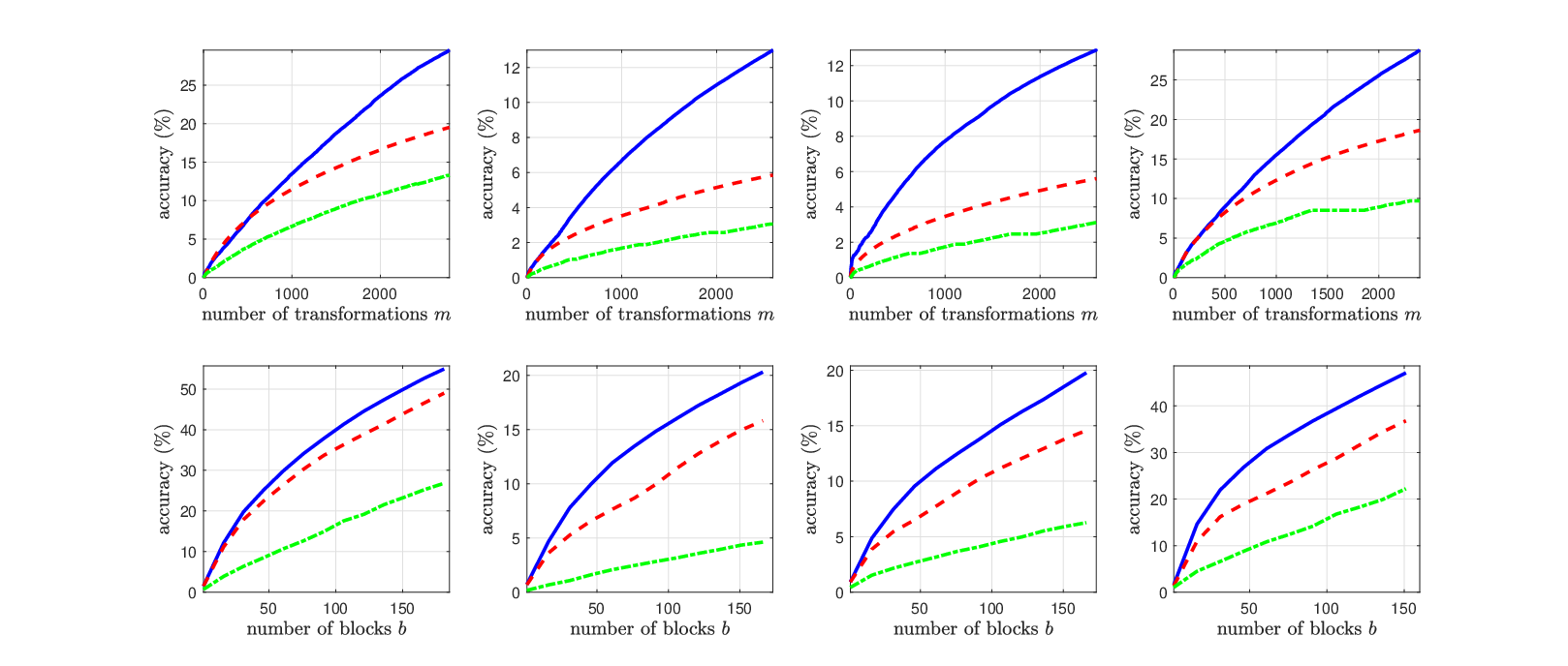
In this section we provide experimental results using popular datasets from the machine learning community to highlight the performance of the proposed method11 1 https://github.com/cristian-rusu-research/JACOBI-SVD. We use the following datasets: ISOLET22 2 https://www.archive.ics.uci.edu/ml/datasets/isolet with 26 classes and ; USPS33 3 https://www.github.com/darshanbagul/USPS_Digit_Classification with 10 classes and ; EMNIST digits44 4 https://www.nist.gov/itl/iad/image-group/emnist-dataset with 10 classes and ; and EMNIST fashion55 5 https://www.github.com/zalandoresearch/fashion-mnist with 10 classes and .
To measure the performance of the proposed algorithm and competitors, we will use the following accuracy metric:
| (10) |
the denominator represents the sum of the true largest singular values while the numerator is the sum of the first diagonal elements from , i.e., the data matrix after steps of the proposed algorithm have been applied.
In Figure 1 we show the evolution of the error (10) with the number of transformations for both Algorithm 1 and Algorithm 1 - block. For comparisons and reference we show the Kogbetliantz method (indices are chosen to maximize ) and a randomized approach (indices are chosen uniformly at random), respectively. The proposed method performs best, while Kogbetliantz picks many times indices that lead to (see Remark 1). Due to their prevalence in the numerical linear algebra literature [42], we also test against a randomized method that picks indices uniformly at random and then performs the optimal transform on those indices. Similar results are observed irrespective of the choice for .
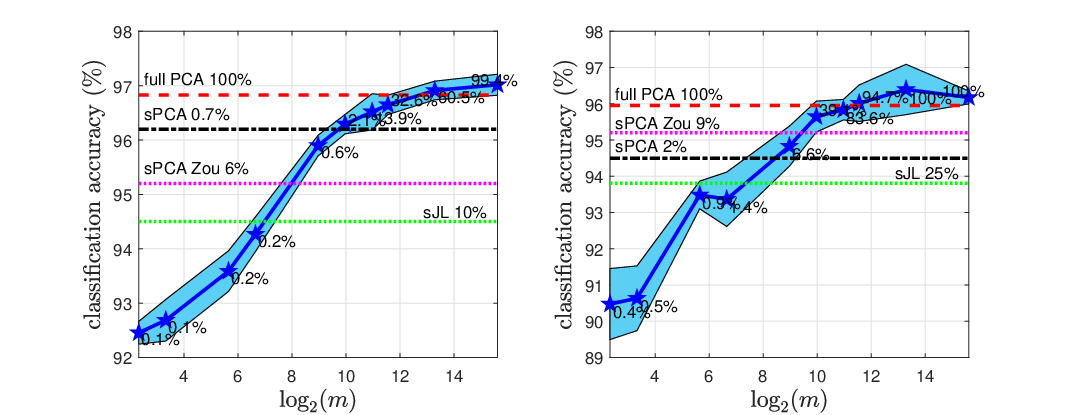
In Figure 2 we show an application of the singular vectors we compute via the proposed method for dimensionality reduction with in a classification scenario. We consider the USPS and MNIST digits datasets for which we use the -Nearest Neighbors (-NN) algorithm with to peform classification. We randomly split the dataset into and for MNIST, and and for USPS. As performance reference, we show the results of the full PCA and the sparse JL (sJL) transforms [43] with non-zeroes per column. All results are averaged over 10 realizations. We also compare against the sparse PCA (sPCA) [19] and one of the earlier approaches (sPCA Zou) [13] from the literature.
It is surprizing how very sparse projections (below fill-in) lead to within a few percentages of the state-of-the-art classification results. Both and were chosen such that the full PCA and -NN lead to the best experimental results.
We report running times for the proposed method below one second when while for the largest , i.e., , we have 300 and 6 seconds for MNIST and USPS, respectively. sPCA takes 540 and 8 seconds while sPCA Zou takes 450 and 6 seconds for MNIST and USPS, respectively. Both previous methods are slower than the proposed method. We would also like to highlight that there are no hyperparameters to tune for Algorithm 1.
IV Conclusions
In this paper, we have proposed a new algorithm to find a few approximate sparse principal components from a data matrix which we have used to perform dimensionality reduction. The proposed method works directly on the data matrix and does not explicitly build the covariance matrix of the data, and is therefore memory efficient. Numerical results that build sparse principal components and then perform dimensionality reduction with application to classification show that the method is practical and compares very well against the state-of-the-art literature, especially in the running time.
References
- [1] L. N. Trefethen and D. Bau, Numerical Linear Algebra, SIAM, 1997.
- [2] I. M. Johnstone, A. Y. Lu, B. Nadler, D. M. Witten, T. Hastie, R. Tibshirani, and J. O. Ramsay, “On consistency and sparsity for principal components analysis in high dimensions [with comments],” Journal of the American Statistical Association, vol. 104, no. 486, pp. 682–703, 2009.
- [3] F. Zhang, X. Ye, and W. Liu, “Image decomposition and texture segmentation via sparse representation,” IEEE Signal Processing Letters, vol. 15, pp. 641–644, 2008.
- [4] D. Schmitter and M. Unser, “Landmark-based shape encoding and sparse-dictionary learning in the continuous domain,” IEEE Transactions on Image Processing, vol. 27, no. 1, pp. 365–378, 2018.
- [5] Z. Khan, F. Shafait, and A. Mian, “Joint group sparse PCA for compressed hyperspectral imaging,” IEEE Transactions on Image Processing, vol. 24, no. 12, pp. 4934–4942, 2015.
- [6] S. Rambhatla, X. Li, J. Ren, and J. Haupt, “A dictionary-based generalization of robust PCA with applications to target localization in hyperspectral imaging,” IEEE Transactions on Signal Processing, vol. 68, pp. 1760–1775, 2020.
- [7] S. Javed, A. Mahmood, S. Al-Maadeed, T. Bouwmans, and S. K. Jung, “Moving object detection in complex scene using spatiotemporal structured-sparse RPCA,” IEEE Transactions on Image Processing, vol. 28, no. 2, pp. 1007–1022, 2019.
- [8] J. H. Manton, “Optimization algorithms exploiting unitary constraints,” IEEE Transactions on Signal Processing, vol. 50, no. 3, pp. 635–650, 2002.
- [9] A. M. Tillmann, “On the computational intractability of exact and approximate dictionary learning,” IEEE Signal Processing Letters, vol. 22, no. 1, pp. 45–49, 2015.
- [10] J. Cadima and I. T. Jolliffe, “Loading and correlations in the interpretation of principle components,” Journal of Applied Statistics, vol. 22, no. 2, pp. 203–214, 1995.
- [11] I. T Jolliffe, N. T. Trendafilov, and M. Uddin, “A modified principal component technique based on the LASSO,” Journal of Computational and Graphical Statistics, vol. 12, no. 3, pp. 531–547, 2003.
- [12] R. Tibshirani, “Regression shrinkage and selection via the LASSO,” Journal of the Royal Statistical Society. Series B (Methodological), vol. 58, no. 1, pp. 267–288, 1996.
- [13] H. Zou, T. Hastie, and R. Tibshirani, “Sparse principal component analysis,” Journal of Computational and Graphical Statistics, vol. 15, no. 2, pp. 265–286, 2006.
- [14] A. d’Aspremont, L. El Ghaoui, M. I. Jordan, and G. R. G. Lanckriet, “A direct formulation for sparse PCA using semidefinite programming,” SIAM Review, vol. 49, no. 3, pp. 434–448, 2007.
- [15] A. d’Aspremont, F. Bach, and L. El Ghaoui, “Optimal solutions for sparse principal component analysis,” J. Mach. Learn. Res., vol. 9, pp. 1269–1294, June 2008.
- [16] M. O. Ulfarsson and V. Solo, “Sparse variable PCA using geodesic steepest descent,” IEEE Transactions on Signal Processing, vol. 56, no. 12, pp. 5823–5832, 2008.
- [17] S. Bartelmaos and K. Abed-Meraim, “Fast principal component extraction using Givens rotations,” IEEE Signal Processing Letters, vol. 15, pp. 369–372, 2008.
- [18] H. Shen and J. Z. Huang, “Sparse principal component analysis via regularized low rank matrix approximation,” Journal of Multivariate Analysis, vol. 99, no. 6, pp. 1015–1034, 2008.
- [19] M. Hein and T. Bühler, “An inverse power method for nonlinear eigenproblems with applications in 1-spectral clustering and sparse PCA,” in NIPS, 2010.
- [20] M. Journée, Y. Nesterov, P. Richtárik, and R. Sepulchre, “Generalized power method for sparse principal component analysis,” J. Mach. Learn. Res., vol. 11, pp. 517–553, Mar. 2010.
- [21] Z. Ma, “Sparse principal component analysis and iterative thresholding,” The Annals of Statistics, vol. 41, no. 2, pp. 772–801, 2013.
- [22] P. Xiao and L. Balzano, “Online sparse and orthogonal subspace estimation from partial information,” in 2016 54th Annual Allerton Conference on Communication, Control, and Computing (Allerton), 2016, pp. 284–291.
- [23] B. Minnehan and A. Savakis, “Grassmann manifold optimization for fast L1-norm principal component analysis,” IEEE Signal Processing Letters, vol. 26, no. 2, pp. 242–246, 2019.
- [24] K. Uchida and I. Yamada, “An ell1-penalization of adaptive normalized quasi-Newton algorithm for sparsity-aware generalized eigenvector estimation,” in 2018 IEEE Statistical Signal Processing Workshop (SSP), 2018, pp. 528–532.
- [25] M. Weylandt, “Multi-rank sparse and functional PCA manifold optimization and iterative deflation techniques,” in 2019 IEEE 8th International Workshop on Computational Advances in Multi-Sensor Adaptive Processing (CAMSAP), 2019, pp. 500–504.
- [26] J. Song, P. Babu, and D. Palomar, “Sparse generalized eigenvalue problem via smooth optimization,” IEEE Transactions on Signal Processing, vol. 63, pp. 1627–1642, 2015.
- [27] K. Benidis, Y. Sun, P. Babu, and D. P. Palomar, “Orthogonal sparse PCA and covariance estimation via Procrustes reformulation,” IEEE Transactions on Signal Processing, vol. 64, no. 23, pp. 6211–6226, 2016.
- [28] A. Breloy, S. Kumar, Y. Sun, and D. P. Palomar, “Majorization-minimization on the Stiefel manifold with application to robust sparse PCA,” IEEE Transactions on Signal Processing, vol. 69, pp. 1507–1520, 2021.
- [29] M. R. Hestenes, “Inversion of matrices by biorthogonalization and related results,” Journal of the Society for Industrial and Applied Mathematics, vol. 6, no. 1, pp. 51–90, 1958.
- [30] J. Götze, P. Rieder, and J. A. Nossek, “Implementation of Kogbetliantz’s SVD algorithm using orthonormal -rotations,” in 1996 8th European Signal Processing Conference (EUSIPCO 1996), 1996, pp. 1–4.
- [31] J. G. McWhirter, “An algorithm for polynomial matrix SVD based on generalised Kogbetliantz transformations,” in 2010 18th European Signal Processing Conference, 2010, pp. 457–461.
- [32] M. O. Ulfarsson and V. Solo, “Selecting the number of principal components with SURE,” IEEE Signal Processing Letters, vol. 22, no. 2, pp. 239–243, 2015.
- [33] P. Schonemann, “A generalized solution of the orthogonal Procrustes problem,” Psychometrika, vol. 31, no. 1, pp. 1–10, 1966.
- [34] C. Rusu and J. Thompson, “Learning fast sparsifying transforms,” IEEE Trans. Sig. Proc., vol. 65, no. 16, pp. 4367–4378, 2017.
- [35] C. Rusu and L. Rosasco, “Fast approximation of orthogonal matrices and application to PCA,” arXiv:1907.08697, 2019.
- [36] P. Schonemann, “On two-sided orthogonal Procrustes problems,” Psychometrika, vol. 33, no. 1, pp. 19–33, 1968.
- [37] C. Jacobi, “Uber ein leichtes Verfahren die in der Theorie der Sacularstorungen vorkommenden Gleichungen numerisch aufzulosen,” Journal fur die reine und angewandte Mathematik, vol. 30, pp. 51–94, 1846.
- [38] J. Charlier, M. Vanbegin, and P. V. Dooren, “On efficient implementations on Kogbetliantz’s algorithm for computing the singular value decomposition,” Numerische Mathematik, vol. 52, no. 3, pp. 279–300, 1988.
- [39] R. A. Horn and C. R. Johnson, Matrix analysis, Cambridge University Press, 2013.
- [40] C. Rusu and L. Rosasco, “Constructing fast approximate eigenspaces with application to the fast graph Fourier transforms,” arXiv:2002.09723, 2020.
- [41] C. Rusu, “An iterative Jacobi-like algorithm to compute a few sparse eigenvalue-eigenvector pairs,” arXiv:2105.14642, 2021.
- [42] P. Drineas and M. W. Mahoney, “RandNLA: Randomized numerical linear algebra,” Commun. ACM, vol. 59, no. 6, pp. 80–90, 2016.
- [43] D. M. Kane and J. Nelson, “Sparser Johnson-Lindenstrauss transforms,” J. ACM, vol. 61, no. 1, 2014.