Seeking SUSY fixed points in the expansion Preprint: DESY 21-114
Abstract
We use the expansion to search for fixed points corresponding to dimensional =1 Wess-Zumino models of scalar superfields interacting through a cubic superpotential. In the case we classify all SUSY fixed points that are perturbatively unitary. In the and cases, we focus on fixed points where the scalar superfields form a single irreducible representation of the symmetry group (irreducible fixed points). For we show that the S5 invariant super Potts model is the only irreducible fixed point where the four scalar superfields are fully interacting. For , we go through all Lie subgroups of O(5) and then use the GAP system for computational discrete algebra to study finite subgroups of O(5) up to order 800. This analysis gives us three fully interacting irreducible fixed points. Of particular interest is a subgroup of O(5) that exhibits O(3)/Z2 symmetry. It turns out this fixed point can be generalized to a new family of models, with and O(N)/Z2 symmetry, that exists for arbitrary integer N.
1 Introduction
In recent years, dimensional superconformal field theories (SCFTs) with minimal () supersymmetry have received significant attention Grover:2013rc; Bashkirov:2013vya; Fei:2016sgs; Bashmakov:2018wts; Benini:2018bhk; Gaiotto:2018yjh; Benini:2018umh; Rong:2018okz; Atanasov:2018kqw; Rong:2019qer. Perhaps the simplest model with this symmetry is the so-called super-Ising model, which was proposed in Grover:2013rc to describe a quantum critical point at the boundary of a dimensional topological superconductor. Because the super-Ising model preserves time reversal symmetry, its spectrum contains only one relevant operator which is time-reversal invariant. This means that a generic renormalization group flow (not necessarily supersymmetric) can reach the fixed point by tuning a single parameter. This property is called emergent supersymmetry and might be realizable in experiment.
Apart from the super-Ising, a whole zoo of theories have been identified and they are sometimes related by dualities Bashmakov:2018wts; Benini:2018bhk; Gaiotto:2018yjh; Benini:2018umh. In particular, a certain super QED was shown to be dual to an Wess-Zumino model Benini:2018bhk; Gaiotto:2018yjh. This duality has many proprieties that resemble the self duality of non-supersymmetric QED coupled to two complex scalars, which describes the famous de-confinement quantum critical point senthil2004deconfined; wang2017deconfined.
The study of dimensional SCFT has also been boosted by technical improvements on standard techniques. For example, it was observed in Fei:2016sgs that if one sets the number of Dirac fermions to in four dimensions, after analytic continuation to dimensions, one ends up with a single three-dimensional Majorana fermion when . By studying the Gross-Neveu-Yukawa model with Dirac fermions and one real scalar, one gets a perturbative fixed-point which is in good agreement with the super-Ising model in dimensions. This technique can be easily generalized to more general dimensional Wess-Zumino models with superpotential11 1 The quadratic terms break time-reversal symmetry and cannot be added to the superpotential (see for example Gaiotto:2018yjh).
| (1.1) |
In other words, one can study the corresponding Gross-Neveu-Yukawa model
| (1.2) |
with .
Parallel to these analytical developments, progress has also been made using the highly successful numerical bootstrap program Rattazzi:2008pe; Poland:2018epd. Recent works that studied dimensional SCFTs using numerical techniques include Bashkirov:2013vya; Rong:2018okz; Atanasov:2018kqw; Rong:2019qer. In particular, when applied to the super-Ising model, the scaling dimension of the superfield can be determined to very high precision Rong:2018okz.
In this work we would like to find an organizational scheme for three-dimensional models with supersymmetry. Our analysis will be perturbative and rely in the standard -expansion. The logic being that a one-loop analysis should give us at least a qualitative understanding of potential fixed points. Once we know a fixed point exists, and have a basic idea of its spectrum, we can use more powerful techniques like the modern numerical bootstrap in order to solve it to high precision. This work is then similar to Osborn:2017ucf; Codello:2019isr; Osborn:2020cnf, where scalar models in several dimensions were studied using a similar method.
Our approach is then the following, we use the expansion to search for SCFTs with a small number of scalar superfields interacting through the superpotential (1.1). We systematically study all the cases when the number scalar superfields is less or equal than 5. In Section 3, we start with the case, which will also include all the possible solutions for . For the superpotential has 10 independent couplings , by solving the one-loop beta functions we list in Table 1 all the possible fixed points with that are perturbatively unitary. We then increase the number of scalar to in Section 4 and to in Section 5. We focus on the SUSY fixed points where the scalar superfields form a single irreducible representation of the symmetry group. We call these fixed points “irreducible fixed points”. This means the coupling constants are a linear superposition of the degree three invariant tensors of the symmetry group. The invariant tensors are traceless and also satisfy
| (1.3) |
This is essentially the trace condition used in Brezin:1973jt, and has important physical consequences. It implies there is only one boson mass operator that is invariant under the symmetry group of the fixed points. For the most stable fixed point of the beta function, this operator is also the only relevant operator that preserves both time-reversal symmetry and the flavor symmetry of the SCFT. Similar to the super-Ising model, non-supersymmetric RG flows will reach the supersymmetric fixed point as long as one tunes the coupling of the boson mass term to zero. In other words, these systems have emergent supersymmetry. The results of the classification are listed in Table 2. In the case, it turns out that there is only one group that gives us a fixed point where the four superfields are fully interacting. This result is based on the analysis of all the subgroups of O(4) in michel1981landau. In the case, we focus on Lie subgroups and finite subgroups of O(5) with orders less or equal to 800. In Section 6, we observe that some fixed points for low values of can be considered the first entry in a family of fixed points that can be generalized to higher values of . For example, the O(3)/Z2 SCFT presented in Table 2 can be generalized to a new family of SCFTs preserving the O(N)/Z2 symmetry. This family complements the three families (the super Potts models, the SU(N) invariant SCFTs and the F4-family of SCFTs) of Wess-Zumino models already studied in Rong:2019qer.
| and ’s | Symmetry | |||
|---|---|---|---|---|
| 1 | (3.3) | -19.7392 | ||
| 2 | (3.4) | S3 | -92.1163 | |
| (3.5) | , | Z2 | -39.2973 | |
| 3 | (3.6) | , , | S4 | -82.9047 |
| (3.7) | , , | O(2) | -144.941 | |
| (3.8) | S3 | -58.6635 | ||
| (3.9) | , , | K4=Z2 Z2 | -110.647 | |
| (3.10) | Z2 | -58.8549 | ||
| (3) | Z2 | -101.963 |
| Symmetry | ||||
|---|---|---|---|---|
| 4 | S5 | -97.5349 | Section 4.1 | |
| 5 | S6 | -115.145 | Section 5.3 | |
| S5 | -207.262 | |||
| O(3)/Z2 | -322.407 |
2 General proprieties of the SCFTs
The one-loop beta function of the SCFT Wess-Zumino model with scalar superfields coupled through the superpotential (1.1) is given by Fei:2016sgs,
| (2.1) |
and the anomalous dimension matrix (whose eigenvalues give us the anomalous dimension) reads
| (2.2) |
Like the scalar theory in dimensions, this is a gradient flow Grinstein:2014xba; Osborn:2017ucf; Codello:2019isr. In other words,
| (2.3) |
with
| (2.4) |
Along the RG flow to the IR, decreases and at the fixed points,
| (2.5) |
Here are the eigen-values of the anomalous dimension matrix.
3 reducible fixed points
The strategy we employ in this section is identical to the one described in Codello:2019isr to study scalar theory in dimensions. Notice that the coupling constant is a fully symmetric tensor and can be characterized as
| (3.1) |
Here is symmetry and traceless. We parameterize the potential as
| (3.2) | |||||
The parameterization relies on the representation theory of O(3). The couplings
form a representation of O(3) with respectively. Clearly, forms a vector representation of O(3). We can use the and rotation to set ,and after that we can use to set . After fixing the redundant O(3) rotations solution of are discrete. The super Ising model plus two decoupled free scalar superfields is located at
| (3.3) |
and all other ’s and’s vanishing.
The S3 invariant fixed point (S3 super Potts model) of two scalars plus a decoupled scalar superfield is located at
| (3.4) |
and all other ’s and’s vanishing. The Lagrangian of the super Potts model can in fact be re-written as an =2 supersymmetric Lagrangian with a single complex chiral superfield Rong:2018okz. This explains the anomalous dimension
The Z2 fixed point with two coupled scalars plus one decoupled scalar superfield is located at
| (3.5) |
and all other ’s and’s vanishing.
The S4 invariant super Potts model is located at
| (3.6) |
and all other ’s and’s vanishing.
The O(2) fixed point with the three scalars fully coupled is located at
| (3.7) |
and all other ’s and’s vanishing.
The S3 invariant fixed point with all three scalars fully coupled is located at
| (3.8) |
and all other ’s and’s vanishing.
The K4 invariant fixed point with all three scalars fully coupled is located at
| (3.9) |
and all other ’s and’s vanishing.
The Z2 invariant fixed point with all three scalars fully coupled is located at
| (3.10) |
and all other ’s and’s vanishing. .
Finally, another Z2 invariant fixed point with all three scalars fully coupled is located at
| (3.11) |
A summary of the previous analysis is presented in Table 1. We can compare our results with the perturbative fixed points of scalar theory in dimension, which were studied in Codello:2019isr. Our entries of Table 1 turn out to be in one-to-one correspondence with the fixed points of scalar theory in dimensions. In dimensions, only the O(2) fixed point and the K4 fixed point are perturbatively unitary. In our case, it seems that supersymmetry improves the situation a lot, and all the fixed points become perturbatively unitary.
4 irreducible fixed points
We now discuss the case when the scalar superfield transforms as an irreducible representation of the symmetry group. To construct the superpotential (1.1), the symmetry group needs to preserve a rank-3 fully symmetric invariant tensor . The tensors are necessarily traceless, such that the representation is reducible. Another important condition is that the invariant tensors satisfy22 2 Otherwise one can build projectors of the form (4.1) which projects the vector representation into invariant subspace. Here is the first eigenvalue of .
| (4.2) |
This is analogous to the trace condition used in Brezin:1973jt. We can now normalize to satisfy
| (4.3) |
If the symmetry group preserves a single , the beta function and the anomalous dimension become
| (4.4) |
Here is defined through
| (4.5) |
assuming satisfies the normalization (4.3). Using the fact that
| (4.6) |
one can prove that
| (4.7) |
From the beta function (4), we know that the one-loop fixed point exists if and only if
| (4.8) |
The irreducible subgroups of O(4) were studied extensively in michel1981landau. It was discovered that only five of the groups have a four dimensional irreducible real representation that preserves a degree three polynomial 33 3 The representation is irreducible when the fields are real, but can be reducible when they are complex. In that case, the representation equals the sum of two complex conjugate representations.. The result is recalled in Table 3. The five polynomials are
| (4.9) |
| SmallGroup Id | subgroup | order | invariant polynomial |
|---|---|---|---|
| [120,34] | S5 | 120 | |
| [72,40] | (S3S3) Z2 | 72 | |
| [36,10] | S3 S3 | 36 | |
| [20,3] | Z5 Z4 | 20 | |
| [18,4] | (Z3Z3) Z2 | 18 | and |
The corresponding fully symmetric invariant tensor can be easily constructed from these polynomials
| (4.10) |
Of these five polynomials only two of them are independent. We can pick these two independent polynomials to be and . The polynomial is related to by an O(3) rotation. The group that preserves is Z5Z4, which is, in fact, a subgroup of S5 (which preserves ). The two groups have the same degree three polynomial but different degree four polynomials. This means that to break the symmetry from S5 to Z5Z4, it is necessary to include quartic terms in the superpotential (1.1). Since we include only cubic terms (the quartic terms are not only irrelevant, but also break time-reversal symmetry), the symmetry of our Lagrangian will be S5. Also, is related to by an O(3) rotation. Including either or in the superpotential (1.1) will preserve the symmetry (S3S3)Z2. The subgroup (Z3Z3) Z2 preserves two polynomials and . However, any combination of the two polynomial can be brought back to the form by an O(3) rotation (the rotation parameter depends on a and b). This means a superpotential of the form in fact preserves the symmetry (S3S3)Z2 at any of point of the -plane. This of course is also true for the SCFT fixed point.
4.1 The fixed points and anomalous dimensions
We can now use the explicit form of the polynomial to study the S5 invariant fixed point. Plug into (4.10), re-scale it to satisfy the normalization (4.3), and then plug it in (4.5), we get
| (4.11) |
Since , the fixed point exists, and from (4) we know
| (4.12) |
This model belongs to the family of =1 Potts models studied in Rong:2019qer.
Similarly, we can also use the polynomial to study the (S3S3)Z2 invariant fixed point, we get
| (4.13) |
Since , the fixed point exists, and we get
| (4.14) |
Consider a superpotential , we know that
| (4.15) |
with
| (4.16) |
So that the model is simply two decoupled copies of the S3 super Potts model.
5 irreducible fixed points
5.1 The Lie group O(3)
Among the Lie subgroups of O(5), there is only one subgroup where the 5 dimensional vector irrep remains irreducible. This is the group O(3), under this embedding, the 5 of O(5) become the T irrep of O(3).44 4 We denote the symmetric traceless, antisymmetric and singlet irrep of O(N) by T, A and S respectively. The invariant tensor of such a representation can be constructed using the of O(3), we will postpone the details of the construction to Section 6.2, where we discuss the generalization of this fixed point to a series SCFTs with the scalar superfields transforming in the T irrep of O(N). We note down here the constant,
| (5.1) |
Since , the one-loop fixed point exists, the anomalous dimension is
| (5.2) |
and the corresponding A function reads
| (5.3) |
Notice the Z2 transformation
| (5.4) |
acts trivially on the T irrep of O(3), so that the symmetry of the fixed point is
| (5.5) |
5.2 Finite subgroups of O(5) up to order 800 with 5 dimensional faithful irreps
We now use the GAP system GAP4 for computational discrete algebra and the Small Groups library eick2018smallgrp to search for finite groups with 5 dimensional faithful irreducible representations, similar to the study done in Ludl:2010bj. Since all representations of finite groups are unitary representations, these finite groups are subgroups of U(5). There are two theorems that are especially useful in seeking faithful irreducible representations Ludl:2010bj.
- •
Theorem 1 Suppose a finite group G has a p dimensional irreducible representation, then Ord(G)/p is an integer.
- •
Theorem 2 Suppose a finite group G has a p dimensional faithful irreducible representation, then this irreducible representation has a single character p in the character table.
The proof of Theorem 1 can be found in hall2018theory Page 288. The proof of Theorem 2 was given in Ludl:2010bj Appendix A.1. The SmallGroup library allows one to specify a finite group using two integers , the first integer indicates the order of the group, while the second integer enumerates all finite groups with order . We first select finite groups that are not Abelian. For example, the following command
| l := Filtered( AllSmallGroups(60) ,x - IsAbelian(x)=false);; | (5.6) |
gives all non-Abelian groups with order 60. The GAP system also allows us to calculate the character table easily
| (5.7) |
To select 5 dimensional irreps, we can use
| (5.8) |
The symbol psi is now a list which contains all the characters of the 5 dimensional irreps:
| gap psi[1]; | |||
| Character( CharacterTable( Alt( [ 1 .. 5 ] ) ), [ 5, -1, 1, 0, 0 ] ) | (5.9) |
The characters contain a single 5, so according to Theorem 2 this is a faithful irrep. It is sometimes useful to check the structure description of the finite group
| (5.10) |
From the output, we learn that SmallGroup(60,5) is the alternating group of five elements, or “A5”. Since our goal is to search for degree 3 invariant polynomials, we can also use the command
| MolienSeries(psi[1]); | (5.11) |
to obtain the Molien Series of the corresponding irrep. The Molien series
| (5.12) |
is a generating function which counts the number of invariant polynomials of a certain degree. Here is the order of the group G, is a representation of G. Doing a series expansion of , the coefficient of counts the number of invariant polynomials of degree n. The Molien series of the five-dimensional irrep of A5 is
| (5.13) |
So that it has one degree two invariant polynomial, two degree three polynomials and two degree four polynomials.
There are more than finite groups of order less or equal than 800. Among them, we found only 109 groups that have at least one 5 dimensional faithful irrep. They are listed in Table 5. Among these 109 finite groups, it turns out 13 of them are also subgroups of O(5). That is, the finite groups preserve a bilinear form, or in other words, their Molien series takes the form
| (5.14) |
These groups are marked with an “*” in Table 5. Among the 13 finite subgroups of O(5), only four of them have irreducible representations that preserve at least one degree three invariant polynomial. The results are listed in Table 4. For a fixed , bigger groups tend to preserve less invariant polynomials, which leads us to conjecture that this list is complete.55 5 We actually extended the analysis up to order 1000 and our final result does not change.
| ID | Group | Irrep | Molien Series | Molien Series (expansion) |
|---|---|---|---|---|
| [60, 5] | A5 | 5 | ||
| [120, 34] | S5 | |||
| [360,188] | A6 | |||
| 5’ | ||||
| [720,763] | S6 | |||
| 5’ |
5.2.1 The group A5
The SmallGroup([60,5]) is the alternating group of five elements. As is explicit from the Molien series, it has a five dimensional irrep, which has a degree two invariant polynomial and two degree five polynomial. To work out the explicit form of the polynomial, after running command (5.8), we can use
| IrreducibleRepresentationsDixon( SmallGroup(60,5),psi[1] ); | (5.15) |
to calculate a matrix representation of the generators of the group
| (5.16) |
Here (1,2,3,4,5) and (1,2,3) denote the cyclic permutations that generate the alternating group. We can now calculate the invariant tensor using these matrices, for example, we can use the Mathematica function “NullSpace[ ]”. Notice that the generators from “IrreducibleRepresentationsDixon” are not necessarily orthogonal. The bi-linear form
| (5.17) |
that is preserved by and is not proportional to the identity matrix. To fix this, we perform the Cholesky Decomposition of . Then the new representation of the generators in terms of the orthogonal matrices is
| (5.18) |
In this basis, we found the two degree three invariant polynomials to be
| (5.19) | |||||
and
| (5.20) | |||||
5.2.2 The group S5
The permutation group of five elements has two five dimensional irreps denoted by the Young diagram and . For simplicity, we will denote them as and . The group A5 can be embedded in S5 through the standard way. That is, S5 contains all the permutations of five elements, while A5 contains even permutation that permutes the five elements. Under this embedding, both and branch into the 5 dimensional irrep of A5.
| (5.21) |
One can similarly work out the invariant polynomials by using the generators from “IrreducibleRepresentationsDixon”. It turns out that the invariant polynomial of is related to by an O(5) rotation, while the invariant polynomial of is related to by an O(5) rotation.
5.2.3 The group A6 and S6
The group S6 contains all permutations of six elements. There are two 5 dimensional irreps that preserve a degree-three polynomial. One of them is the standard irreps of permutation groups “”. We will denote the other irrep as “”. As is clear from Table 4, the two irreps in fact have the same Molien series. This is only possible if the two irreps have exactly the same invariant polynomials. Physically, this means a potential with transforms in the irrep can be also interpreted as a potential with transforms in the irrep.
The symmetric group S5 can be embedded in S6 in the standard way. While S6 contains all the permutation that permutes six elements, S5 contains all the permutation that permutes five of the six elements. Under this embedding
| (5.22) |
An invariant polynomial of the parent group S6 should also be an invariant polynomial of the subgroup S5. We, therefore, know the degree three invariant polynomial of is simply . Since and have the same Molien series, the invariant polynomial of should also be .
From Table 4, we know the Molien series of the group A6 and S6 are the same up to terms. Physically, this means we can not break the symmetry from S6 to A5 until we introduce terms in the (super-)potential. Since we consider only cubic terms of the superpotential, we should consider only the group S6.
5.3 The beta functions and fixed points
We can now consider the beta function of the =1 Lagrangian with superpotential
| (5.23) |
with and defined in (5.19) and (5.20). The beta function is
| (5.24) |
and the corresponding anomalous dimension is
| (5.25) |
We find the following four fixed points:
A fixed point at () preserves S5 symmetry. It has and .
A fixed point at () preserves S6 symmetry. It has and .
A fixed point at () instead of the A5 symmetry, preserves O(3)/Z2 symmetry. The superpotential takes the form
| (5.26) |
The polynomial
| (5.27) |
is related to the invariant polynomial of O(3)/Z2 by an O(5) rotation. It has and . This fixed point is the most stable one. These A5 invariant RG flows have an IR fixed point with emergent O(3)/Z2 symmetry.
6 Generalization to higher
6.1 SN SN bi-standard fixed points
We discuss here the irreducible fixed points first. The decoupled S3 Potts model studied in Section 4.1 can also be understoodd as an SCFT with the four scalar superfields transforming in the bi-standard representation of S3 S3. This SCFT can be easily generalized to a higher number of scalar superfields, if we take the scalars to transform in the representation of . The constant defined in (4.5) is simply the product of the ’s of the individual ’s,
| (6.1) |
Interestingly, if we take , and if is an even number,
| (6.2) |
The one-loop =1 SUSY fixed point is guaranteed to exist. Take the group to be SN SN, we have then , so that
| (6.3) |
Also the A-function is
| (6.4) |
6.2 O(N)/Z2 fixed points
We now try to generalize the O(3)/Z2 fixed studied in Section 5.1 to a family of fixed points with O(N)/Z2 symmetry. The scalar superfields carry indices in the T irrep of O(N), so that these fixed points have interacting scalar superfields. The product of two vector irreps of O(N) can be decomposed into the S, A and T irreps:
The projector to the T irrep is
| (6.5) |
Here we use the birdtrack notation Cvitanovic:2008zz. Solid lines mean the Kronecker , the unfilled box means symmetrization, and the filled box means anti-symmetrization. The invariant tensor for the T irrep of O(N) is simply,
| (6.6) |
We rescale the invariant tensor to satisfy the normalization (4.3), which can now be represented as
| (6.7) |
After contracting the Kronecker delta’s, we get
| (6.8) |
with
| (6.9) |
Notice for , which satisfies the condition (4.8). So that the fixed points exist at one loop. The anomalous dimension is then
| (6.10) |
The A-function is
| (6.11) |
As already mentioned in Section 5.1, since the scalar superfields carry an O(N) T index, the central element of O(N)
| (6.12) |
acts trivially on . The flavor symmetry of the SCFTs is then
| (6.13) |
6.3 Generalization of A5
The group A5 is very interesting. As far as we know, this is the first example of a group that has an irrep that satisfies the trace condition (preserves a single degree two polynomial) and preserves more than one degree three polynomial. To generalize this to the higher-component case we use the birdtrack technique Cvitanovic:2008zz. To be more specific, we search for subgroups of SN groups that have an irrep with the Molien series
| (6.14) |
Again we decompose two vector irreps of O(n) as S, A and T. If a subgroup of O(n) preserves a rank three symmetric traceless tensor, the T irrep of O(n) gets further decomposed into two irreps:
![[Uncaptioned image]](2107.14515v1/twoline.png)
|
(6.15) | ||||
The invariant tensor of the standard irrep of SN satisfies a special condition. That is, the A irrep of O(n) does not decompose. In term of birdtracks, it implies the following identity:
| (6.16) |
Here
is the dimension of the standard irrep of SN. The coefficient is fixed by contracting the top two legs. From the above relation we can show that the invariant tensor of SN satisfies
| (6.17) |
with
| (6.18) |
We now want to generalize the group A5 to a group with higher . According to the Molien series, we first introduce another invariant tensor
| (6.19) |
The Molien series also tells us that the irrep has only two degree four invariant polynomials. This means the two invariant tensors satisfy
| (6.20) |
and
| (6.21) |
Contracting two legs with , we get
| (6.22) |
Where we have used the normalization conditions,
![[Uncaptioned image]](2107.14515v1/bubble1.png)
|
|||||
![[Uncaptioned image]](2107.14515v1/bubble2.png)
|
|||||
![[Uncaptioned image]](2107.14515v1/bubble3.png)
|
(6.23) |
Contracting two legs of (6.20) with
![[Uncaptioned image]](2107.14515v1/v1.png) , we get
, we get
| (6.24) |
with
| (6.25) |
From this we can prove
| (6.26) |
The proof is given in Appendix A.
Contracting two legs of (6.20) with
![[Uncaptioned image]](2107.14515v1/v2.png) , we get
, we get
| (6.27) |
with
| (6.28) |
Contracting two legs of (6.21) with
, we obtain
| (6.29) |
Since the two tensor are independent, we get
| (6.30) |
According to (6.25), this leads to
| (6.31) |
Using (6.20) and (6.21), after a long calculation, we get
| (6.32) |
From this we know how the anti-symmetric subspace can be decomposed using the projectors:
| (6.33) |
and
| (6.34) |
They satisfy
| (6.35) |
The dimension of the corresponding irrep is
| (6.36) |
We can calculate the diagram
| (6.37) |
Here we use
![[Uncaptioned image]](2107.14515v1/P2P2nCG.png) to denote the Clebsch–Gordan coefficients of .
This diagram is a sum of squares,
to denote the Clebsch–Gordan coefficients of .
This diagram is a sum of squares,
| (6.38) |
and is therefore non-negative. This puts a constraint on the values that can take. Notice that is a positive integer, so that
| (6.39) |
The dimensions of the irreps and also need to be positive integers, there are only two solutions of these Diophantine conditions, they are
| (6.40) |
The solution corresponds to the group A5 we have studied, while the solution might correspond to a subgroup of S27.
Let us assume that such a group exists and calculate the beta function and anomalous dimensions. Take the superpotential to be
| (6.41) |
using the birdtrack relations (6.24), (6.26) and (6.27), we get
| (6.42) |
and the corresponding anomalous dimension is
| (6.43) |
We find the following fixed points:
A fixed point at () has and .
A fixed point at () preserves S27 symmetry. It has and .
A fixed point at () has and .
Notice the birdtrack rules (6.20) and (6.21) are very similar to the rules that lead to the classification of the F4-family of Lie groups, see Cvitanovic:2008zz equation (19.16). Other birdtrack conditions lead to the classification of E6, E7 and E8 family of Lie Groups. Deligne conjectured that there exist categories interpolating these exceptional groups deligne1996serie; deligne2002exceptional. See Binder:2019zqc for how to use the Deligne category to make sense of O(N) invariant quantum field theories at non-integer N. It is tempting to conjecture that (6.20) and (6.21) also lead to a new Deligne category. We leave this for future work.
6.4 The =1 Potts models
The =1 Potts models were already studied in Rong:2019qer. We recall here the procedure to construct the invariant tensor according to Zia:1975ha. In Rong:2019qer, the were constructed explicitly and used to calculated to two loops in . The result was shown to be consistent with the result from the non-perturbative bootstrap. Take the scalar superfield to transform in the dimensional standard representation of SN. First, we need to construct with and . The is a vector in the dimensional Euclidean space . The index labels the vertices of a hypertetrahedron. The can be constructed through a recursion relation,
| (6.44) | |||||
with . Here is the set of N-1 vectors in . The recursion starts with and . The invariant tensor is defined as,
| (6.45) |
The overall constant is chosen so that the invariant tensor satisfies the normalization (4.3). From the above definition of , we get
| (6.46) |
and
| (6.47) |
6.5 Generalization of reducible fixed points
Take the superpotential to be
| (6.48) |
The functions for the three coupling turn out to be
| (6.49) |
The anomalous dimension is given by
| (6.50) |
The constant is defined in (4.5). Take to be the invariant tensor of the standard irrep of SN (6.45). At
| (6.51) | |||||
| (6.52) | |||||
| (6.53) |
the scalar superfield and together form the dimensional standard representation of . This corresponds to the Potts model studied in the previous subsection.
6.5.1 The O(N-1) fixed points with with
When , for any value of N, there exists only one perturbatively unitary O(N-1) invariant fixed point with real coupling constant. This has been studied in Benini:2018bhk. The scalar superfields transform in the vector representation of O(N-1) while is invariant under an O(N-1) transformation. The value of the coupling at the fixed can be worked out analytically. It is however rather complicated and not very illuminating. Let us record here the large N result,
| (6.54) |
The anomalous dimension is given by
| (6.55) |
The A-function is
| (6.56) |
In three dimensions, the large N limit of the fixed points is dual to =1 higher-spin theory on AdS4 through AdS/CFT correspondence Leigh:2003gk; Sezgin:2003pt.
6.5.2 SN fixed point with
The fixed point is located at
| (6.57) | |||||
| (6.58) | |||||
| (6.59) |
(There are three equivalent fixed points related to the above one by field re-definition.) The scalar superfields transform in the N-1 dimensional standard representation representation of SN while is invariant under SN transformation. The anomalous dimension is given by
| (6.60) |
The A-function is
| (6.61) |
Notice there exists a non-conformal window given by
| (6.62) |
within which the fixed point is non-unitary. The upper edge of the window is . At the edges of the window
| (6.63) |
Clearly, at the lower edge of the non-conformal window, the fixed point collides with the decoupled SN Potts models and one free scalar theory. At the upper edge of the non-conformal window the fixed point collides with the O(N-1) invariant fixed point.
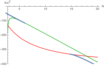
The beta functions (6.5) have a few other fixed points. They are, however, decoupled combinations of either the super-Ising model, SN Potts model, or the free theory. We will not list them here.
7 Discussion
A natural generalization of the =1 analysis of this paper is to study =2 SCFTs. Consider the following =2 superpotential
| (7.1) |
The function is given by
| (7.2) |
and the anomalous dimension matrix reads
| (7.3) |
The scalar superfield is complex so that the coupling transform in the fully symmetric representation of U(N). By studying subgroups of U(N) and analyzing their degree three invariant polynomials we can study the corresponding =2 superconformal fixed points. Among the 109 finite subgroups of U(5) with 5 dimensional faithful irreducible representations, we found a single group whose Molien Series takes the form
| (7.4) |
The group has a SmallGroup id [180,19] and structure description GL(2,4). This is the general linear group of degree two over the field of four elements. Notice that the corresponding irrep has no degree two invariant polynomials, it is in fact a complex irrep. This irrep has two degree three polynomials. Using these two polynomials to construct an =2 superpotential as in (7.1), and analyzing the beta function, we get a full conformal manifold. The group GL(2,4) is in fact the direct product of A5 and cyclic group of order three Z3. The invariant polynomials of GL(2,4) are simply and as defined in (5.19) and (5.20). The five variables are now complex. The action of Z3 is
| (7.5) |
It might be interesting to study this conformal manifold in more detail. A similar study of a conformal manifold containing the XYZ model was performed in Baggio:2017mas.
Notice the degree three invariant polynomials studied in this paper can be used to construct a Landau theory with cubic terms. The Landau criterion says that a second-order phase transition is possible only if the irrep of the order parameter has no degree three invariant polynomials. This however is known to fail in two dimensions. For example, the 3 state Potts model is known to go through a second order phase transition at the critical temperature. The corresponding Landau theory with a cubic term has an infra-red conformal fixed point. It will be interesting to understand whether the Landau theories analogous to the SCFTs studied in this paper lead to unitary conformal field theories in two dimensions. The problem perhaps can be studied using conformal bootstrap techniques.
Due to the special form of the superpotential (1.1), we focus here on finite subgroups of O(4) and O(5) which preserve degree three invariant polynomials. It will also be interesting to study degree four polynomials, which can then be used to construct theories in dimensions. The early works in the 80’s focused on theories where the scalars form a single irreducible representation of the symmetry group. In michel1981landau; toledano1985renormalization, all the subgroups of O(4) and the corresponding theories were studied extensively. The work of hatch1985selection; kim1986classification; hatch1986renormalization; stokes1987continuous studied the theories with N=6 and N=8 scalars forming irreducible representations of the 230 crystallographic space groups (see also stokes1988isotropy). Recently, there was also revived interest on fixed points of reducible theories where the scalars form more than one irrep of the symmetry groups Osborn:2017ucf; Rychkov:2018vya; Hogervorst:2020gtc; Osborn:2020cnf. Some of these perturbative fixed points were shown to survive in three dimensions using the numerical bootstrap Rong:2017cow; Stergiou:2018gjj; Kousvos:2018rhl; Stergiou:2019dcv; Kousvos:2019hgc; Henriksson:2020fqi; Henriksson:2021lwn. A full classification of the irreducible theories with N scalars will need the classification of subgroups of O(N), this can be difficult when N is large. The method used in Section 5.2 based on the GAP system can be easily generalized to study theories. It will be interesting to see whether we can discover new fixed points in the expansion.
As mentioned in the introduction, the numerical bootstrap method has proven to be very powerful in studying dimensional =1 SCFTs. In particular, the work of Rong:2019qer studied three infinite families of Wess-Zumino models. It will be interesting to apply the numerical bootstrap to the new O(N)/Z2 family discovered in this work. As usual, due to the non-perturbative nature of the numerical bootstrap, we expect rigorous numerical results that can then be compared to other methods such as the -expansion. We leave this interesting analysis for future work.
| [ 55, 1 ], C11 C5 | *[ 60, 5 ], A5 |
|---|---|
| *[ 80, 49 ], (C2 C2 C2 C2) C5 | [ 110, 2 ], C2 (C11 C5) |
| *[ 120, 34 ], S5 | *[ 120, 35 ], C2 A5 |
| [ 125, 3 ], (C5 C5) C5 | [ 125, 4 ], C25 C5 |
| [ 155, 1 ], C31 C5 | *[ 160, 234 ], ((C2 C2 C2 C2) C5) C2 |
| *[ 160, 235 ], C2 ((C2 C2 C2 C2) C5) | [ 165, 1 ], C3 (C11 C5) |
| [ 180, 19 ], GL(2,4) | [ 205, 1 ], C41 C5 |
| [ 220, 2 ], C4 (C11 C5) | [ 240, 91 ], A5 C4 |
| [ 240, 92 ], C4 A5 | *[ 240, 189 ], C2 S5 |
| [ 240, 199 ], C3 ((C2 C2 C2 C2) C5) | [ 250, 8 ], ((C5 C5) C5) C2 |
| [ 250, 10 ], C2 ((C5 C5) C5) | [ 250, 11 ], C2 (C25 C5) |
| [ 275, 1 ], C11 C25 | [ 275, 3 ], C5 (C11 C5) |
| [ 300, 22 ], C5 A5 | [ 305, 1 ], C61 C5 |
| [ 310, 2 ], C2 (C31 C5). | [ 320, 1583 ], ((C2 C2 C2 C2) C5) C4 |
| [ 320, 1584 ], C4 ((C2 C2 C2 C2) C5) | *[ 320, 1635 ], ((C2 C2 C2 C2) C5) C4 |
| *[ 320, 1636 ], C2 (((C2 C2 C2 C2) C5) C2) | [ 330, 4 ], C6 (C11 C5) |
| [ 355, 1 ], C71 C5 | *[ 360, 118 ], A6 |
| [ 360, 119 ], C3 S5 | [ 360, 122 ], C6 A5 |
| [ 375, 2 ],((C5 C5) C5) C3 | [ 375, 4 ], C3 ((C5 C5) C5) |
| [ 375, 5 ], C3 (C25 C5) | [ 385, 1 ], C7 (C11 C5) |
| [ 400, 52 ], (C2 C2 C2 C2) C25 | [ 400, 213 ], C5 ((C2 C2 C2 C2) C5) |
| [ 405, 15 ], (C3 C3 C3 C3) C5 | [ 410, 2 ], C2 (C41 C5) |
| [ 420, 13 ], C7 A5 | [ 440, 2 ], C8 (C11 C5) |
| [ 465, 2 ], C3 (C31 C5) | [ 480, 217 ], A5 C8 |
| [ 480, 220 ], C8 A5 | [ 480, 943 ], C4 S5 |
| [ 480, 1194 ] , C3 (((C2 C2 C2 C2) C5) C2) | [ 480, 1204 ], C6 ((C2 C2 C2 C2) C5) |
| [ 495, 1 ], C9 (C11 C5) | [ 500, 11 ], ((C5 C5) C5) C4 |
| [ 500, 13 ], C4 ((C5 C5) C5) | [ 500, 14 ], C4 (C25 C5) |
| [ 500, 25 ], ((C5 C5) C5) C4 | [ 500, 33 ], C2 (((C5 C5) C5) C2) |
| [ 505, 1 ], C101 C5 | [ 540, 31 ], C9 A5 |
| [ 550, 2 ] C2 (C11 C25) | [ 550, 10 ], C10 (C11 C5) |
| [ 560, 173 ] C7 ((C2 C2 C2 C2) C5) | [ 600, 144 ], C5 S5 |
| [ 600, 147 ], C10 A5 | [ 605, 1 ], C121 C5 |
| [ 605, 3 ], C11 (C11 C5) | [ 605, 5 ], (C11 C11) C5 |
| [ 605, 6 ], (C11 C11) C5 | [ 610, 2 ], C2 (C61 C5) |
| [ 615, 1 ], C3 (C41 C5) | [ 620, 2 ]C4 (C31 C5) |
| [ 625, 6 ], C125 C5. | [ 625, 7 ], (C5 C5 C5) C5 |
| [ 625, 8 ], (C25 C5) C5 | [ 625, 9 ], (C25 C5) C5 |
| [ 625, 10 ], (C25 C5) C5 | [ 625, 14 ], (C25 C5) C5 |
| [ 640, 19097 ], ((C2 C2 C2 C2) C5) C8 | [ 640, 19103 ], C8 ((C2 C2 C2 C2) C5) |
| [ 640, 21456 ], ((C2 C2 C2 C2) C5) C8 | [ 640, 21458 ], C4 (((C2 C2 C2 C2) C5) C2) |
| *[ 640, 21536 ], C2 (((C2 C2 C2 C2) C5) C4) | [ 655, 1 ], C131 C5 |
| [ 660, 4 ], C12 (C11 C5) | [ 660, 13 ], PSL(2,11) |
| [ 660, 14 ], C11 A5 | [ 710, 2 ], C2 (C71 C5) |
| [ 715, 1 ], C13 (C11 C5) | [ 720, 399 ], C9 ((C2 C2 C2 C2) C5) |
| [ 720, 412 ], C3 (A5 C4) | [ 720, 419 ], C12 A5 |
| *[ 720, 763 ], S6 | *[ 720, 766 ], C2 A6 |
| [ 720, 769 ], C6 S5 | [750,6], ((C5 C5) C5) C6 |
| [750,7], C2 (((C5 C5) C5) C3) | [750,13], C3 (((C5 C5) C5) C2) |
| [750,24], C6 ((C5 C5) C5) | [750,25], C6 (C25 C5) |
| [755,1], C151 C5 | [770, 4], C14 (C11 C5) |
| [775,1], C31 C25 | [780,13], C13 A5 |
| [800,384], C2 ((C2 C2 C2 C2) C25) | [800,1195], C5 (((C2 C2 C2 C2) C5) C2) |
| [800,1203], C10 ((C2 C2 C2 C2) C5) |
Acknowledgments
J. R. would like to thank Ning Su for discussions, and Andreas Stergiou for introducing to him the GAP system during the “Bootstrap 2019” conference held at Perimeter Institute. The work of P. L. and J. R. is supported by the DFG through the Emmy Noether research group “The Conformal Bootstrap Program” project number 400570283.
Appendix A Proof of (6.27)
![[Uncaptioned image]](2107.14515v1/v1p.png)
![[Uncaptioned image]](2107.14515v1/temp2.png)
References
- (1) T. Grover, D. Sheng and A. Vishwanath, Emergent Space-Time Supersymmetry at the Boundary of a Topological Phase, Science 344 (2014) 280 [1301.7449].
- (2) D. Bashkirov, Bootstrapping the SCFT in three dimensions, 1310.8255.
- (3) L. Fei, S. Giombi, I.R. Klebanov and G. Tarnopolsky, Yukawa CFTs and Emergent Supersymmetry, PTEP 2016 (2016) 12C105 [1607.05316].
- (4) V. Bashmakov, J. Gomis, Z. Komargodski and A. Sharon, Phases of theories in 2 + 1 dimensions, JHEP 07 (2018) 123 [1802.10130].
- (5) F. Benini and S. Benvenuti, = 1 QED in 2 + 1 dimensions: dualities and enhanced symmetries, JHEP 05 (2021) 176 [1804.05707].
- (6) D. Gaiotto, Z. Komargodski and J. Wu, Curious Aspects of Three-Dimensional SCFTs, JHEP 08 (2018) 004 [1804.02018].
- (7) F. Benini and S. Benvenuti, = 1 dualities in 2+1 dimensions, JHEP 11 (2018) 197 [1803.01784].
- (8) J. Rong and N. Su, Bootstrapping the minimal = 1 superconformal field theory in three dimensions, JHEP 06 (2021) 154 [1807.04434].
- (9) A. Atanasov, A. Hillman and D. Poland, Bootstrapping the Minimal 3D SCFT, JHEP 11 (2018) 140 [1807.05702].
- (10) J. Rong and N. Su, Bootstrapping the = 1 Wess-Zumino models in three dimensions, JHEP 06 (2021) 153 [1910.08578].
- (11) T. Senthil, A. Vishwanath, L. Balents, S. Sachdev and M.P. Fisher, Deconfined quantum critical points, Science 303 (2004) 1490.
- (12) C. Wang, A. Nahum, M.A. Metlitski, C. Xu and T. Senthil, Deconfined quantum critical points: symmetries and dualities, Physical Review X 7 (2017) 031051.
- (13) R. Rattazzi, V.S. Rychkov, E. Tonni and A. Vichi, Bounding scalar operator dimensions in 4D CFT, JHEP 12 (2008) 031 [0807.0004].
- (14) D. Poland, S. Rychkov and A. Vichi, The Conformal Bootstrap: Theory, Numerical Techniques, and Applications, Rev. Mod. Phys. 91 (2019) 015002 [1805.04405].
- (15) H. Osborn and A. Stergiou, Seeking fixed points in multiple coupling scalar theories in the expansion, JHEP 05 (2018) 051 [1707.06165].
- (16) A. Codello, M. Safari, G.P. Vacca and O. Zanusso, Symmetry and universality of multifield interactions in dimensions, Phys. Rev. D 101 (2020) 065002 [1910.10009].
- (17) H. Osborn and A. Stergiou, Heavy handed quest for fixed points in multiple coupling scalar theories in the expansion, JHEP 04 (2021) 128 [2010.15915].
- (18) E. Brezin, J.C. Le Guillou and J. Zinn-Justin, DISCUSSION OF CRITICAL PHENOMENA IN MULTICOMPONENT SYSTEMS, Phys. Rev. B 10 (1974) 892.
- (19) L. Michel, J. Toledano and P. Toledano, Landau free energies for n= 4 and the subgroups of o (4), Symmetries and broken symmetries in condensed matter physics (1981) .
- (20) B. Grinstein, D. Stone, A. Stergiou and M. Zhong, Challenge to the Theorem in Six Dimensions, Phys. Rev. Lett. 113 (2014) 231602 [1406.3626].
- (21) The GAP Group, GAP – Groups, Algorithms, and Programming, Version 4.11.1, 2021.
- (22) B. Eick, H. Besche and E. O’Brien, Smallgrp—the gap small groups library, GAP package, version 1 (2018) .
- (23) P.O. Ludl, On the finite subgroups of U(3) of order smaller than 512, J. Phys. A 43 (2010) 395204 [1006.1479].
- (24) M. Hall, The theory of groups, Courier Dover Publications (2018).
- (25) P. Cvitanovic, Group theory: Birdtracks, Lie’s and exceptional groups (2008).
- (26) P. Deligne, La série exceptionnelle de groupes de lie, Comptes Rendus de l’Academie des Sciences-Serie I-Mathematique 322 (1996) 321.
- (27) P. Deligne and B.H. Gross, On the exceptional series, and its descendants, Comptes Rendus Mathematique 335 (2002) 877.
- (28) D.J. Binder and S. Rychkov, Deligne Categories in Lattice Models and Quantum Field Theory, or Making Sense of Symmetry with Non-integer , JHEP 04 (2020) 117 [1911.07895].
- (29) R.K.P. Zia and D.J. Wallace, Critical Behavior of the Continuous N Component Potts Model, J. Phys. A 8 (1975) 1495.
- (30) R.G. Leigh and A.C. Petkou, Holography of the N=1 higher spin theory on AdS(4), JHEP 06 (2003) 011 [hep-th/0304217].
- (31) E. Sezgin and P. Sundell, Holography in 4D (super) higher spin theories and a test via cubic scalar couplings, JHEP 07 (2005) 044 [hep-th/0305040].
- (32) M. Baggio, N. Bobev, S.M. Chester, E. Lauria and S.S. Pufu, Decoding a Three-Dimensional Conformal Manifold, JHEP 02 (2018) 062 [1712.02698].
- (33) J.-C. Toledano, L. Michel, P. Toledano and E. Brezin, Renormalization-group study of the fixed points and of their stability for phase transitions with four-component order parameters, Physical Review B 31 (1985) 7171.
- (34) D.M. Hatch, H.T. Stokes, J.S. Kim and J.W. Felix, Selection of stable fixed points by the toledano-michel symmetry criterion: Six-component example, Physical Review B 32 (1985) 7624.
- (35) J.S. Kim, D.M. Hatch and H.T. Stokes, Classification of continuous phase transitions and stable phases. i. six-dimensional order parameters, Physical Review B 33 (1986) 1774.
- (36) D.M. Hatch, J.S. Kim, H.T. Stokes and J.W. Felix, Renormalization-group classification of continuous structural phase transitions induced by six-component order parameters, Physical Review B 33 (1986) 6196.
- (37) H.T. Stokes, J.S. Kim and D.M. Hatch, Continuous solid-solid phase transitions driven by an eight-component order parameter: Hamiltonian densities and renormalization-group theory, Physical Review B 35 (1987) 388.
- (38) H.T. Stokes and D.M. Hatch, Isotropy subgroups of the 230 crystallographic space groups, World Scientific (1988).
- (39) S. Rychkov and A. Stergiou, General Properties of Multiscalar RG Flows in , SciPost Phys. 6 (2019) 008 [1810.10541].
- (40) M. Hogervorst and C. Toldo, Bounds on multiscalar CFTs in the expansion, JHEP 04 (2021) 068 [2010.16222].
- (41) J. Rong and N. Su, Scalar CFTs and Their Large N Limits, JHEP 09 (2018) 103 [1712.00985].
- (42) A. Stergiou, Bootstrapping hypercubic and hypertetrahedral theories in three dimensions, JHEP 05 (2018) 035 [1801.07127].
- (43) S.R. Kousvos and A. Stergiou, Bootstrapping Mixed Correlators in Three-Dimensional Cubic Theories, SciPost Phys. 6 (2019) 035 [1810.10015].
- (44) A. Stergiou, Bootstrapping MN and Tetragonal CFTs in Three Dimensions, SciPost Phys. 7 (2019) 010 [1904.00017].
- (45) S.R. Kousvos and A. Stergiou, Bootstrapping Mixed Correlators in Three-Dimensional Cubic Theories II, SciPost Phys. 8 (2020) 085 [1911.00522].
- (46) J. Henriksson, S.R. Kousvos and A. Stergiou, Analytic and Numerical Bootstrap of CFTs with Global Symmetry in 3D, SciPost Phys. 9 (2020) 035 [2004.14388].
- (47) J. Henriksson and A. Stergiou, Perturbative and Nonperturbative Studies of CFTs with MN Global Symmetry, SciPost Phys. 11 (2021) 015 [2101.08788].