跳到论文正文
W Papers独立论文阅读器 arXiv:2107.14371 论文正文 计算阅读时间 · 0%
引用这篇论文根据当前论文元数据生成,正式投稿前建议核对。


License: arXiv.org perpetual non-exclusive license
arXiv:2107.14371v1 [math.OC] 29 Jul 2021

Distributed Strategy Selection: A Submodular Set Function Maximization Approach

Navid Rezazadeh Affiliation: Mechanical and Aerospace Eng. Dept. Affiliation: University of California Irvine Affiliation: Irvine, CA Email: nrezazad@uci.edu    Solmaz S. Kia Affiliation: Mechanical and Aerospace Eng. Dept. Affiliation: University of California Irvine Affiliation: Irvine, CA Email: solmaz@uci.edu
Abstract

Constrained submodular set function maximization problems often appear in multi-agent decision-making problems with a discrete feasible set. A prominent example is the problem of multi-agent mobile sensor placement over a discrete domain. Submodular set function optimization problems, however, are known to be NP-hard. This paper considers a class of submodular optimization problems that consist of maximization of a monotone and submodular set function subject to a uniform matroid constraint over a group of networked agents that communicate over a connected undirected graph. We work in the value oracle model where the only access of the agents to the utility function is through a black box that returns the utility function value. We propose a distributed suboptimal polynomial-time algorithm that enables each agent to obtain its respective strategy via local interactions with its neighboring agents. Our solution is a fully distributed gradient-based algorithm using the submodular set functions’ multilinear extension followed by a distributed stochastic Pipage rounding procedure. This algorithm results in a strategy set that when the team utility function is evaluated at worst case, the utility function value is in 1c​(1−e−c−O⁡(1/T))\frac{1}{c}(1-{\textup{e}}^{-c}-O(1/T)) of the optimal solution with cc to be the curvature of the submodular function. An example demonstrates our results.

1 Introduction

This paper studies a multi-agent optimal planning in discrete space, which is often referred to as optimal strategy scheduling. We consider a group of 𝒜={1,…,N}\mathcal{A}\!=\!\{1,...,N\} agents with communication and computation capabilities, interacting over a connected undirected graph 𝒢⁡(𝒜,ℰ)\mathcal{G}(\mathcal{A},\mathcal{E}). Each agent i∈𝒜i\in\mathcal{A} has a distinct discrete strategy set 𝒫i\mathcal{P}_{i}, known only to agent ii, and wants to choose at most κi∈ℤ>0\kappa_{i}\in\mathbb{Z}_{>0} strategies from 𝒫i\mathcal{P}_{i} such that a monotone increasing and submodular utility function f:2𝒫→ℝ≥0f:2^{\mathcal{P}}\to{\mathbb{R}}_{\geq 0}, 𝒫=⋃i∈𝒜𝒫i\mathcal{P}\!=\!\bigcup\nolimits_{i\in\mathcal{A}}\mathcal{P}_{i}, evaluated at all the agents’ strategy selection is maximized11 1 We use standard notation, but for clarity we provide a brief description of the notation and the definitions in Section 2.. In other words, the agents aim to solve in a distributed manner the discrete domain optimization problem

maxℛ∈ℐ​f​(ℛ)\displaystyle\underset{\mathcal{R}\in\mathcal{I}}{\textup{max}}f(\mathcal{R}) (1a)
ℐ={ℛ⊂𝒫\displaystyle\mathcal{I}=\big\{\mathcal{R}\subset\mathcal{P}\, ||ℛ∩𝒫i|≤κi,∀i∈𝒜}.\displaystyle\big|\,\,|\mathcal{R}\cap\mathcal{P}_{i}|\leq\kappa_{i},~\forall i\in\mathcal{A}\big\}. (1b)

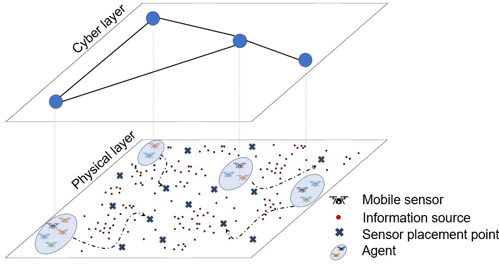
The agents’ access to the utility function is through a black box that returns f⁡(ℛ)f(\mathcal{R}) for any given set ℛ∈𝒫\mathcal{R}\in\mathcal{P} (value oracle model). The constraint set (1b) is a partition matroid, which restricts the number of strategy choices of each agent i∈𝒜i\in\mathcal{A} to κi\kappa_{i}. In a distributed solution, each agent i∈𝒜i\in\mathcal{A} should obtain its respective component ℛi⋆∈𝒫i\mathcal{R}^{\star}_{i}\in\mathcal{P}_{i} of ℛ⋆=∪j=1Nℛ⋆j\mathcal{R}^{\star}=\cup_{j=1}^{N}\mathcal{R}^{\star}_{j}, the optimal solution of (1), by interacting only with the agents that are in its communication range. Optimization problem (1) is known to be NP hard GLN-LAW-MLF:78. Our goal is to design a polynomial-time distributed solution for (1) with formal guarantees on the optimality bound. Our problem is motivated by a wide range of multi-agent exploration, and sensor placement problems for monitoring and coverage, which can be formulated in the form of submodular maximization problem (1) NR-SSK:21; AH-MG-HV-UT:20; VT-AJ-GJP:16; XD-MG-RP-FB:20; SW-CGC:20; SA-EF-LSL:14. An example application scenario is shown in Fig. 1.

When the utility function of (1) is monotone increasing and submodular set function, the sequential greedy algorithm MLF-GLN-LAW:78 delivers a polynomial-time suboptimal solution with guaranteed optimality bound. The sequential greedy algorithm is a central solution. Several attempts have been undertaken to adapt the sequential greedy algorithm for large-scale submodular maximization problems by reducing the size of the problem through approximations KW-RI-JB:14 or using several processing units to achieve a faster sequential greedy algorithm, however, with some sacrifices on the optimality bound BM-AK-RS-AK:13; BM-MZ-AK:16; RK-BM-SV-AV:15; PSR-OS-MF:20. Decentralized implementation of the sequential greedy algorithm through sequential message passing or via sequential message sharing through a cloud is also discussed in NR-SSK:21.

The optimality gap achieved by sequential greedy algorithm for problem (1) is 11+c​f​(ℛ⋆)\frac{1}{1+c}\,f(\mathcal{R}^{\star}) MC-GC:84, where cc is the curvature of the utility function. More recently, another suboptimal solution for problem (1) with an improved optimality gap is proposed in the literature using the multilinear continuous relaxation of a submodular set function JV:08; AAB-BM-JB-AK:17; AM-HH-AK:20; OS-MF:20. The relaxation transforms the discrete problem (1) into a continuous optimization problem with linear constraints. Then, a continuous gradient-based optimization algorithm is used to solve the continuous optimization problem. A suboptimal solution for (1) with the improved optimality gap of 1c​(1−e−c)​f​(ℛ⋆)\frac{1}{c}(1-{\textup{e}}^{-c})\,f(\mathcal{R}^{\star}) then is obtained by properly rounding the continuous-domain solution JV:10. This approach however requires a central authority to solve the problem. In sensor placement problems, when the agents are self-organizing autonomous mobile agents with communication and computation capabilities, it is desired to solve the optimization problem 1 in a distributed way, without involving a central authority. For the special case of zero curvature, and when each agent has only one choice to make, i.e., κi=1\kappa_{i}=1 for all i∈𝒜i\in\mathcal{A}, AR-AA-BS-JGP-HH:19 has proposed an average consensus-based distributed algorithm to solve the multi-linear extension relaxation of 1 over connected graphs. The solution of AR-AA-BS-JGP-HH:19 requires exact knowledge of the multi-linear extension function. However, the computational complexity of constructing the exact value of the multi-linear extension of a submodular function and its derivatives is exponential in the size of the strategy set. The result in AR-AA-BS-JGP-HH:19 also requires a centralized rounding scheme.

The multi-linear extension function of a submodular function, as we review in Section 2.2, is equivalently the expected value of the submodular function evaluated at random sets obtained by picking strategies from the strategy set independently with a probability. This stochastic interpretation has allowed approximating the multi-linear extension function and its derivatives emphatically with a reasonable computational cost via sampling from the strategy set. This approach has been used JV:10 in its continuous domain solution of submodular optimization problems. Of course, as expected, this approach comes with a penalty on the optimality gap that is inversely proportional to the number of the samples.

In this paper, motivated by the improved optimality gap of the multilinear continuous relaxation-based algorithms, we develop a distributed implementation of the algorithm of JV:10 over a connected undirected graph to obtain a suboptimal solution for (1). We propose a gradient-based algorithm, which uses a maximum consensus message passing scheme over the communication graph. We complete our solution by designing a fully distributed rounding procedure to compute the final suboptimal strategy of each agent. In this algorithm, to manage the computational cost of constructing the multilinear extension of the utility function, we use a sampling-based evaluation of the multilinear extension. Through rigorous analysis, we show that our proposed distributed algorithm in finite time TT achieves, with a known probability, a 1c​(1−e−c)−O⁡(1/T)\frac{1}{c}(1-{\textup{e}}^{-c})-O(1/T) optimality bound, where 1/T1/T is the step size of the algorithm and the frequency at which agents communicate over the network. A numerical example demonstrates our results.

2 Preliminaries

This section introduces our notation and relevant definitions from graph theory and submodular set functions22 2 Since we use standard notation, the reader familiar with the subject can continue to Section 3 and come back to this section if the need arises..

2.1 Notion

We denote the vectors with bold small font. The pthp^{\textup{th}} element of vector 𝐱\boldsymbol{\mathbf{x}} is denoted by [𝐱]p[\boldsymbol{\mathbf{x}}]_{p}. We denote the inner product of two vectors 𝐱\boldsymbol{\mathbf{x}} and 𝐲\boldsymbol{\mathbf{y}} with appropriate dimensions by 𝐱.𝐲\boldsymbol{\mathbf{x}}.\boldsymbol{\mathbf{y}}. We use 𝟏\boldsymbol{\mathbf{1}} as a vector of ones, whose dimension is understood from the context. We denote sets with the capital curly font. Given a ground set 𝒫={1,⋯,n}\mathcal{P}=\{1,\cdots,n\}, we define the membership probability vector 𝐱∈[0,1]n\boldsymbol{\mathbf{x}}\in[0,1]^{n} to obtain ℛ𝐱⊂𝒫\mathcal{R}_{\boldsymbol{\mathbf{x}}}\subset\mathcal{P} as a random set where p∈𝒫p\in\mathcal{P} is in ℛ𝐱\mathcal{R}_{\boldsymbol{\mathbf{x}}} with the probability [𝐱]p[\boldsymbol{\mathbf{x}}]_{p}. For ℛ⊂𝒫\mathcal{R}\subset\mathcal{P}, 𝟏ℛ∈{0,1}n\boldsymbol{\mathbf{1}}_{\mathcal{R}}\in\{0,1\}^{n} is the vector whose pthp^{\textup{th}} element is 11 if p∈ℛp\in\mathcal{R} and 00 otherwise; we call 𝟏ℛ\boldsymbol{\mathbf{1}}_{\mathcal{R}} the membership indicator vector of set ℛ\mathcal{R}. Given a finite countable set ℛ⊂ℝ\mathcal{R}\subset{\mathbb{R}} and integer κ\kappa, 1≤κ<|ℛ|1\leq\kappa<|\mathcal{R}|, max⁡(ℛ,κ)\max(\mathcal{R},\kappa) returns the κ\kappa largest elements of ℛ\mathcal{R}. |x||x| is the absolute value of x∈ℝx\in{\mathbb{R}}. By overloading the notation, we also use |ℛ||\mathcal{R}| as the cordiality of set ℛ\mathcal{R}. For a set function f:2𝒫→ℝf:2^{\mathcal{P}}\to{\mathbb{R}}, we define Δf​(p|ℛ)=f⁡(ℛ∪{p})−f⁡(ℛ),ℛ⊂𝒫\Delta_{f}(p|\mathcal{R})=f(\mathcal{R}\cup\{p\})-f(\mathcal{R}),\,\,\mathcal{R}\subset\mathcal{P}. A set function is normalized if f⁡(∅)=0f(\emptyset)=0. Given a set ℱ⊂𝒳×ℝ\mathcal{F}\subset\mathcal{X}\times{\mathbb{R}} and an element (p,α)∈𝒳×ℝ(p,\alpha)\in\mathcal{X}\times{\mathbb{R}} we define the addition operator ⊕\oplus as ℱ⊕{(p,α)}={(u,γ)∈𝒳×ℝ|(u,γ)∈ℱ,u≠p}∪{(u,γ+α)∈𝒳×ℝ|(u,γ)∈ℱ,u=p}∪{(p,α)∈𝒳×ℝ|(p,γ)∉ℱ,γ∈ℝ}\mathcal{F}{\oplus}\{(p,\alpha)\}=\{(u,\gamma)\in\mathcal{X}\times{\mathbb{R}}\,|\,(u,\gamma)\in\mathcal{F},u\not=p\}\cup\{(u,\gamma+\alpha)\in\mathcal{X}\times{\mathbb{R}}\,|\,(u,\gamma)\in\mathcal{F},u=p\}\cup\{(p,\alpha)\in\mathcal{X}\times{\mathbb{R}}\,|\,(p,\gamma)\not\in\mathcal{F},\gamma\in\mathbb{R}\}. Given a collection of sets ℱi∈𝒳×ℝ\mathcal{F}_{i}\in\mathcal{X}\times{\mathbb{R}}, i∈𝒜i\in\mathcal{A}, we define the max-operation over these collection as MAXi∈𝒜​ℱi={(u,γ)∈𝒳×ℝ|(u,γ)∈ℱ¯​ s.t. ​γ=max(u,α)∈ℱ¯​α}\underset{i\in\mathcal{A}}{\textup{MAX}}\,\,\mathcal{F}_{i}=\{(u,\gamma)\in\mathcal{X}\times{\mathbb{R}}|(u,\gamma)\in\bar{\mathcal{F}}\text{~s.t.~}\gamma=\underset{(u,\alpha)\in\bar{\mathcal{F}}}{\textup{max}}\alpha\}, where ℱ¯=⋃i∈𝒜ℱi.\bar{\mathcal{F}}=\bigcup_{i\in\mathcal{A}}\mathcal{F}_{i}.

We denote a graph by 𝒢⁡(𝒜,ℰ)\mathcal{G}(\mathcal{A},\mathcal{E}) where 𝒜\mathcal{A} is the node set and ℰ⊂𝒜×𝒜\mathcal{E}\subset\mathcal{A}\times\mathcal{A} is the edge set. 𝒢\mathcal{G} is undirected if and only is (i,j)∈ℰ(i,j)\in\mathcal{E} means that agents ii and jj can exchange information. An undirected graph is connected if there is a path from each node to every other node in the graph. We denote the set of the neighboring nodes of node ii by 𝒩i={j∈𝒜|(i,j)∈ℰ}\mathcal{N}_{i}=\{j\in\mathcal{A}|(i,j)\in\mathcal{E}\}. We also use d⁡(𝒢)d(\mathcal{G}) to show the diameter of the graph.

2.2 Submodular Functions

A set function f:2𝒫→ℝ≥0f:2^{\mathcal{P}}\to{\mathbb{R}}_{\geq 0} is monotone increasing if f⁡(𝒫1)≤f⁡(𝒫2)f(\mathcal{P}_{1})\leq f(\mathcal{P}_{2}), and submodular if for any p∈𝒫∖𝒫2p\in\mathcal{P}\setminus\mathcal{P}_{2},

Δf​(p|𝒫1)≥Δf​(p|𝒫2),\displaystyle\Delta_{f}(p|\mathcal{P}_{1})\geq\Delta_{f}(p|\mathcal{P}_{2}), (2)

hold for any sets 𝒫1⊂𝒫2⊂𝒫\mathcal{P}_{1}\subset\mathcal{P}_{2}\subset\mathcal{P}. The total curvature of a submodular set function f:2𝒫→ℝ≥0f:2^{\mathcal{P}}\to{\mathbb{R}}_{\geq 0}, which shows the worst-case increase in the value of the function when member pp is added, is defined as

c=1−min𝒮,p∉𝒮​Δf​(p|𝒮)Δf​(p|∅)\displaystyle c=1-\underset{\mathcal{S},p\not\in\mathcal{S}}{\textup{min}}\frac{\Delta_{f}(p|{\mathcal{S}})}{\Delta_{f}(p|\emptyset)} (3)

Note that c∈[0,1]c\in[0,1]; the curvature of c=0c=0 means that the function is modular, i.e., f⁡({p1,p2})=f⁡({p1})+f⁡({p2})f(\{p_{1},p_{2}\})=f(\{p_{1}\})+f(\{p_{2}\}), p1,p2∈𝒫p_{1},p_{2}\in\mathcal{P}, while c=1c=1 means that there is at least a member that adds no value to function ff in a special circumstance. Curvature cc represents a measure of the diminishing return of a set function. Whenever the total curvature is not known, it is rational to assume the worst case scenario and set c=1c=1.

In the rest of this paper, without loss of generality, we assume that the ground set 𝒫\mathcal{P} is equal to {1,⋯,n}\{1,\cdots,n\}. For a submodular function f:2𝒫→ℝ≥0f:2^{\mathcal{P}}\to{\mathbb{R}}_{\geq 0}, its multilinear extension F:[0,1]n→ℝ≥0F:[0,1]^{n}\to{\mathbb{R}}_{\geq 0} in the continuous space is

F⁡(𝐱)=∑ℛ⊂𝒫f⁡(ℛ)​∏p∈ℛ[𝐱]p​∏p∉ℛ(1−[𝐱]p),𝐱∈[0,1]n.\displaystyle F(\boldsymbol{\mathbf{x}})=\!\!\sum_{\mathcal{R}\subset\mathcal{P}}{}\!f(\mathcal{R})\prod_{p\in\mathcal{R}}\![\boldsymbol{\mathbf{x}}]_{p}\prod_{p\not\in\mathcal{R}}\!(1-[\boldsymbol{\mathbf{x}}]_{p}),~~\boldsymbol{\mathbf{x}}\in[0,1]^{n}. (4)

FF in (4) is indeed equivalent to

F⁡(𝐱)=𝔼⁡[f⁡(ℛ𝐱)],\displaystyle F(\boldsymbol{\mathbf{x}})=\mathbb{E}[f(\mathcal{R}_{\boldsymbol{\mathbf{x}}})], (5)

where ℛ𝐱⊂𝒫\mathcal{R}_{\boldsymbol{\mathbf{x}}}\subset\mathcal{P} is a set where each element p∈ℛ𝐱p\in\mathcal{R}_{\boldsymbol{\mathbf{x}}} appears independently with the probabilities [𝐱]p[\boldsymbol{\mathbf{x}}]_{p}. Then, taking the derivatives of F⁡(𝐱)F(\boldsymbol{\mathbf{x}}) yields

∂F∂[𝐱]p​(𝐱)=𝔼⁡[f⁡(ℛ𝐱∪{p})−f⁡(ℛ𝐱∖{p})],\displaystyle\frac{\partial F}{\partial[\boldsymbol{\mathbf{x}}]_{p}}(\boldsymbol{\mathbf{x}})=\mathbb{E}[f(\mathcal{R}_{\boldsymbol{\mathbf{x}}}\cup\{p\})-f(\mathcal{R}_{\boldsymbol{\mathbf{x}}}\setminus\{p\})], (6)

and

∂2F∂[𝐱]p​∂[𝐱]q(𝐱)=𝔼[f(ℛ𝐱∪{p,q})−f(ℛ𝐱∪{q}∖{p})\displaystyle\frac{\partial^{2}F}{\partial[\boldsymbol{\mathbf{x}}]_{p}\partial[\boldsymbol{\mathbf{x}}]_{q}}(\boldsymbol{\mathbf{x}})=\mathbb{E}[f(\mathcal{R}_{\boldsymbol{\mathbf{x}}}\cup\{p,q\})-f(\mathcal{R}_{\boldsymbol{\mathbf{x}}}\cup\{q\}\setminus\{p\})
−f(ℛ𝐱∪{p}∖{q})+f(ℛ𝐱∖{p,q})].\displaystyle\quad\quad\quad\quad-f(\mathcal{R}_{\boldsymbol{\mathbf{x}}}\cup\{p\}\setminus\{q\})+f(\mathcal{R}_{\boldsymbol{\mathbf{x}}}\setminus\{p,q\})]. (7)

To construct F⁡(𝐱)F(\boldsymbol{\mathbf{x}}) and its derivatives we should evaluate f⁡(ℛ)f(\mathcal{R}) for all ℛ∈2𝒫\mathcal{R}\in 2^{\mathcal{P}}. Therefore, when the size of 𝒫\mathcal{P} grows, constructing F⁡(𝐱)F(\boldsymbol{\mathbf{x}}) and its derivatives computationally become intractable. The stochastic interpretation (5) of the multilinear extension and its derivatives offer a mechanism to estimate them with a reasonable computational cost via sampling. Chernoff-Hoeffding’s inequality can be used to quantify the quality of these estimates given the number of samples.

Theorem 2.1 (Chernoff-Hoeffding’s inequality WH:94)

Consider a set of KK independent random variables X1,…,XKX_{1},...,X_{K} where a<Xi<ba<X_{i}<b. Let SK=∑i=1KXiS_{K}=\sum_{i=1}^{K}X_{i}, then

ℙ[|SK−𝔼[SK]|>δ]<2e−2​δ2K​(b−a)2,\displaystyle\mathbb{P}[|S_{K}-\mathbb{E}[S_{K}]|>\delta]<2\,\textup{e}^{-\frac{2\delta^{2}}{K(b-a)^{2}}},

for any δ∈ℝ≥0\delta\in{\mathbb{R}}_{\geq 0}.

Given a ground set 𝒫\mathcal{P}, Partition matroid ℳ\mathcal{M} is defined as ℳ={ℛ⊂𝒫||ℛ∩𝒫i|≤ki,∀i∈𝒜}\mathcal{M}=\{\mathcal{R}\subset\mathcal{P}\big|\,\,|\mathcal{R}\cap\mathcal{P}_{i}|\leq k_{i},\forall i\in\mathcal{A}\}, 1≤κi≤|𝒫i|1\leq\kappa_{i}\leq|\mathcal{P}_{i}| and 𝒜={1,…,N}\mathcal{A}=\{1,\dots,N\}, with ⋃i∈𝒜𝒫i=𝒫\bigcup\nolimits_{i\in\mathcal{A}}\mathcal{P}_{i}=\mathcal{P} and 𝒫i∩𝒫j=∅,i≠j\mathcal{P}_{i}\cap\mathcal{P}_{j}=\emptyset,\,\,i\neq j. The matroid polytop for partition matroid is a convex hull defined as (with abuse of notation)

ℳ={𝐱∈[0,1]n|∑p∈𝒫i[𝐱i]p≤κi,∀i∈𝒜}.\displaystyle\mathcal{M}=\{\boldsymbol{\mathbf{x}}\in[0,1]^{n}\,\big|\,\sum\nolimits_{p\in\mathcal{P}_{i}}{}[\boldsymbol{\mathbf{x}}_{i}]_{p}\leq\kappa_{i},\forall i\in\mathcal{A}\}. (8)

where [𝐱]p,p∈𝒫i[\boldsymbol{\mathbf{x}}]_{p},\,\,p\in\mathcal{P}_{i} associated with membership probability of strategies in 𝒫i\mathcal{P}_{i}, i∈𝒜={1,⋯,N}i\in\mathcal{A}=\{1,\cdots,N\}, we have ∑p∈𝒫i[𝐱]p≤κi\sum_{p\in\mathcal{P}_{i}}[\boldsymbol{\mathbf{x}}]_{p}\leq\kappa_{i}.

The following result is established for the optimal solution of the optimization problem (1)

Lemma 2.1 (JV:10)

Consider the set value optimization problem (1). Suppose f:𝒫→ℝ≥0f:\mathcal{P}\to{\mathbb{R}}_{\geq 0} is an increasing and submodular set function with curvature cc whose multilinear extension is F:[0,1]n→ℝ≥0F:[0,1]^{n}\to{\mathbb{R}}_{\geq 0}. Let ℛ⋆\mathcal{R}^{\star} be the optimizer of (1). Then,

𝟏ℛ⋆.∇F​(𝐱)≥f⁡(ℛ⋆)−c​F​(𝐱),∀𝐱∈ℳ.\displaystyle\boldsymbol{\mathbf{1}}_{\mathcal{R}^{\star}}.\nabla F(\boldsymbol{\mathbf{x}})\geq f(\mathcal{R}^{\star})-c\,F(\boldsymbol{\mathbf{x}}),\quad\forall\boldsymbol{\mathbf{x}}\in\mathcal{M}.

3 Decentralized continuous-domain strategy selection

The utility function ff assigns values to all the subsets of 𝒫=⋃i∈𝒜𝒫i={1,⋯,n}\mathcal{P}\!=\!\bigcup\nolimits_{i\in\mathcal{A}}\mathcal{P}_{i}=\{1,\cdots,n\}. Thus, equivalently, we can regard the set value utility function as a function on the Boolean hypercube {0,1}n\{0,1\}^{n}, i.e., f:{0,1}n→ℝf:\{0,1\}^{n}\to{\mathbb{R}}. Multilinear-extension function F⁡(𝐱)F(\boldsymbol{\mathbf{x}}), given in (4), expands the function evaluation of the utility function to over the space between the vertices of this Boolean hypercube. On the other hand, the matroid polytope ℳ\mathcal{M} is the convex haul of the vertices of the hypercube {0,1}n\{0,1\}^{n} that satisfy the partition matroid constraint (1b). Additionally, note that according to (4), F⁡(𝐱)F(\boldsymbol{\mathbf{x}}) for any 𝐱∈ℳ\boldsymbol{\mathbf{x}}\in\mathcal{M} is a weighted average of values of FF at the vertices of the matriod polytope ℳ\mathcal{M}. Then, equivalently, F⁡(𝐱)F(\boldsymbol{\mathbf{x}}) at any 𝐱∈ℳ\boldsymbol{\mathbf{x}}\in\mathcal{M} is a normalized-weighted average of ff on the strategies satisfying constraint (1b). As such,

f⁡(ℛ⋆)≥F⁡(𝐱),𝐱∈ℳ,\displaystyle f(\mathcal{R}^{\star})\geq F(\boldsymbol{\mathbf{x}}),\,\,\,\boldsymbol{\mathbf{x}}\in\mathcal{M},

which is equivalent to f⁡(ℛ⋆)=max𝐱∈ℳ​F​(𝐱)f(\mathcal{R}^{\star})=\underset{\boldsymbol{\mathbf{x}}\in\mathcal{M}}{\textup{max}}\,\,F(\boldsymbol{\mathbf{x}}), where ℛ⋆\mathcal{R}^{\star} is the optimizer of problem (1) JV:08. Therefore, solving the continuous domain optimization problem

max𝐱∈ℳ​F​(𝐱),\displaystyle\underset{\boldsymbol{\mathbf{x}}\in\mathcal{M}}{\textup{max}}\,\,F(\boldsymbol{\mathbf{x}}), (9)

by using a gradient-based method combined with a proper rounding procedure presents itself as a gateway to solving the optimization problem (1). For instance, the solution proposed in JV:10 to solve (9) is the constrained gradient ascent solver

d​𝐱d​t=𝐯(𝐱)where𝐯(𝐱)=arg⁡max𝐰∈ℳ(𝐰.∇F(𝐱)),\displaystyle\frac{\text{d}\boldsymbol{\mathbf{x}}}{\text{d}t}=\boldsymbol{\mathbf{v}}(\boldsymbol{\mathbf{x}})~~\text{where}~~\boldsymbol{\mathbf{v}}(\boldsymbol{\mathbf{x}})=\underset{\boldsymbol{\mathbf{w}}\in\mathcal{M}}{\arg\max}(\boldsymbol{\mathbf{w}}.\nabla F(\boldsymbol{\mathbf{x}})), (10)

initialized at 𝐱⁡(0)=𝟎\boldsymbol{\mathbf{x}}(0)\!=\!\boldsymbol{\mathbf{0}}. Since ℳ\mathcal{M} is convex and 𝐱⁡(0)=∈ℳ\boldsymbol{\mathbf{x}}(0)\!=\!\boldsymbol{\mathbf{0}}\!\in\!\mathcal{M}, the trajectory t↦𝐱t\!\mapsto\!\boldsymbol{\mathbf{x}} of (10) belongs to ℳ\mathcal{M} for t∈[0,1]t\in[0,1]. Due to Lemma 2.1, ascent direction in (10) satisfies

d​Fd​t=𝐯⁡(𝐱).∇F​(𝐱)≥f⁡(ℛ⋆)−c​F​(𝐱).\displaystyle\frac{\text{d}F}{\text{d}t}=\boldsymbol{\mathbf{v}}(\boldsymbol{\mathbf{x}}).\nabla F(\boldsymbol{\mathbf{x}})\geq f(\mathcal{R}^{\star})-c\,F(\boldsymbol{\mathbf{x}}).

Using the Comparison Lemma HKK-JWG:02 then (10) concludes that F⁡(𝐱⁡(1))≥1c​(1−e−c)​f​(ℛ⋆)F(\boldsymbol{\mathbf{x}}(1))\geq\frac{1}{c}(1-\text{e}^{-c})\,f(\mathcal{R}^{\star}). To complete its suboptimal solution, JV:10 uses Pipage rounding procedure AAA-MIS:04 on 𝐱⁡(1)\boldsymbol{\mathbf{x}}(1) to obtain the suboptimal solution of (1) with optimality gap of 1c​(1−e−c)​f​(ℛ⋆)\frac{1}{c}(1-\text{e}^{-c})\,f(\mathcal{R}^{\star}).

Inspired by the central solver (10), in what follows, we present a practical finite time distributed solution for problem (1). Our solution includes a proper distributed sampling method to obtain a polynomial-time numerical approximation of ∇𝐅​(𝐱)\nabla\boldsymbol{\mathbf{F}}(\boldsymbol{\mathbf{x}}) and also a distributed rounding procedure.

3.1 Distributed Discrete Gradient Ascent Solution

To design a distributed iterative solution for (1), let every agent i∈𝒜i\in\mathcal{A} maintain and evolve a local copy of the membership probability vector as 𝐱i​(t)∈ℝn\boldsymbol{\mathbf{x}}_{i}(t)\in{\mathbb{R}}^{n}. Since 𝒫={1,⋯,n}\mathcal{P}=\{1,\cdots,n\} is sorted agent-wise, we denote 𝐱i​(t)=[𝐱^i​1⊤​(t),⋯,𝐱i​i⊤​(t),⋯,𝐱^i​N⊤​(t)]⊤∈ℝn\boldsymbol{\mathbf{x}}_{i}(t)=[\hat{\boldsymbol{\mathbf{x}}}_{i1}^{\top}(t),\cdots,\boldsymbol{\mathbf{x}}_{ii}^{\top}(t),\cdots,\hat{\boldsymbol{\mathbf{x}}}_{iN}^{\top}(t)]^{\top}\in{\mathbb{R}}^{n} where 𝐱i​i​(t)∈ℝ≥0|𝒫i|\boldsymbol{\mathbf{x}}_{ii}(t)\in{\mathbb{R}}_{\geq 0}^{|\mathcal{P}_{i}|} is the membership probability vector of agent ii’s own strategy with entries of [𝐱i​(t)]p,p∈𝒫i[\boldsymbol{\mathbf{x}}_{i}(t)]_{p},\,\,p\in\mathcal{P}_{i} at iteration t∈{0,1,⋯,T}t\in\{0,1,\cdots,T\}, T∈ℤ>0T\in\mathbb{Z}_{>0}, while 𝐱^i​j​(t)∈ℝ≥0|𝒫j|\hat{\boldsymbol{\mathbf{x}}}_{ij}(t)\in{\mathbb{R}}_{\geq 0}^{|\mathcal{P}_{j}|} is the local estimate of the membership probability vector of agent jj by agent ii with entries of [𝐱i​(t)]p​p∈𝒫j,j∈𝒜∖i[\boldsymbol{\mathbf{x}}_{i}(t)]_{p}\,\,p\in\mathcal{P}_{j},\,\,j\in\mathcal{A}\setminus i. Every agent i∈𝒜i\in\mathcal{A} initializes at 𝐱i​(0)=𝟎\boldsymbol{\mathbf{x}}_{i}(0)=\boldsymbol{\mathbf{0}}.

At time step tt, each agent i∈𝒜i\in\mathcal{A} generates KiK_{i} independent samples {ℛik​(t)}k=1Ki\{\mathcal{R}^{k}_{i}(t)\}_{k=1}^{K_{i}} of random set ℛ𝐱i​(t)\mathcal{R}_{\boldsymbol{\mathbf{x}}_{i}(t)}.

drawn according to membership probability vector 𝐱i​(t)\boldsymbol{\mathbf{x}}_{i}(t) from 𝒫\mathcal{P} and empirically computes gradient vector ∇F​(𝐱i​(t))∈ℝ≥0n\nabla F(\boldsymbol{\mathbf{x}}_{i}(t))\in{\mathbb{R}}_{\geq 0}^{n}, which according to (6) is defined element-wise as

[∇F~​(𝐱i​(t))]p=(∑k=1Kif⁡(ℛik​(t)∪{p})−f⁡(ℛik​(t)∖{p}))/Ki,\displaystyle\left[\widetilde{\nabla F}(\boldsymbol{\mathbf{x}}_{i}(t))\right]_{p}\!\!=\!\!\left(\!\sum_{\,k=1}^{K_{i}}\!f(\mathcal{R}^{k}_{i}(t)\!\cup\!\{p\})\!-\!f(\mathcal{R}^{k}_{i}(t)\!\setminus\!\{p\})\!\!\right)\!\!\Big/\!K_{i}, (11)

p∈𝒫={1,⋯,n}p\in\mathcal{P}=\{1,\cdots,n\}. Hereafter, ∇F~​(𝐱i​(t))\widetilde{\nabla F}(\boldsymbol{\mathbf{x}}_{i}(t)) is the empirical estimate of ∇F​(𝐱i​(t))\nabla F(\boldsymbol{\mathbf{x}}_{i}(t)). The following lemma, whose proof is given in the Appendix B and relies on the Chernoff-Hoeffding’s inequality, can quantify the quality of this estimate.

Lemma 3.1

Consider the set value optimization problem (1). Suppose f:𝒫→ℝ≥0f:\mathcal{P}\to{\mathbb{R}}_{\geq 0} is an increasing and submodular set function and consider its multilinear extension F:[0,1]n→ℝ≥0F:[0,1]^{n}\to{\mathbb{R}}_{\geq 0}. Let ∇F~​(𝐱)\widetilde{\nabla F}(\boldsymbol{\mathbf{x}}) be the estimate of ∇F​(𝐱)\nabla F(\boldsymbol{\mathbf{x}}) that is calculated by taking K∈ℤ>0K\in\mathbb{Z}_{>0} samples of set ℛ𝐱\mathcal{R}_{\boldsymbol{\mathbf{x}}} according to membership probability vector 𝐱\boldsymbol{\mathbf{x}}. Then,

|[∇F~​(𝐱⁡(t))]p−∂F∂[𝐱]p​(𝐱)|≥12​T​f​(ℛ⋆),p∈{1,⋯,n},\displaystyle\!\!\left|\left[\widetilde{\nabla F}(\boldsymbol{\mathbf{x}}(t))\right]_{p}-\frac{{\partial F}}{\partial[\boldsymbol{\mathbf{x}}]_{p}}(\boldsymbol{\mathbf{x}})\right|\!\geq\frac{1}{2T}f(\mathcal{R}^{\star}),~~p\in\{1,\cdots,n\}, (12)

with the probability of 2​e−18​T2​K2\textup{e}^{-\frac{1}{8T^{2}}K}, for any T∈ℤ>0T\in\mathbb{Z}_{>0}.

Let each agent i∈𝒜i\in\mathcal{A} propagate its local probability membership function with step size 1T\frac{1}{T} according to

𝐱i−​(t+1)=𝐱i​(t)+1T​𝐯~i​(t),\displaystyle\boldsymbol{\mathbf{x}}_{i}^{-}(t+1)=\boldsymbol{\mathbf{x}}_{i}(t)+\frac{1}{T}\widetilde{\boldsymbol{\mathbf{v}}}_{i}(t), (13)

where

𝐯~i​(t)=argmax𝐰∈ℳi​𝐰.∇F~​(𝐱i​(t))\displaystyle\widetilde{\boldsymbol{\mathbf{v}}}_{i}(t)=\underset{\boldsymbol{\mathbf{w}}\in\mathcal{M}_{i}}{\textup{argmax}}\,\boldsymbol{\mathbf{w}}.\widetilde{\nabla F}(\boldsymbol{\mathbf{x}}_{i}(t)) (14)

with

ℳi={𝐰∈[0,1]n| 1⊤.𝐰≤κi,[𝐰]p=0,∀p∈𝒫\𝒫i}.\displaystyle\mathcal{M}_{i}\!=\!\Big\{\boldsymbol{\mathbf{w}}\!\in\![0,1]^{n}\Big|\,\boldsymbol{\mathbf{1}}^{\top}.\boldsymbol{\mathbf{w}}\leq\kappa_{i}\,\,,[\boldsymbol{\mathbf{w}}]_{p}=0,\,\,\forall p\in\mathcal{P}\backslash\mathcal{P}_{i}\Big\}. (15)

Because the propagation is only based on the local information of agent ii, next, we update the propagated 𝐱i−​(t+1)\boldsymbol{\mathbf{x}}_{i}^{-}(t+1) of each agent i∈𝒜i\in\mathcal{A} by element-wise maximum seeking among its neighbors, i.e.,

𝐱i​(t+1)=maxj∈𝒩i∪{i}​𝐱j−​(t+1).\displaystyle\boldsymbol{\mathbf{x}}_{i}(t+1)=\underset{j\in\mathcal{N}_{i}\cup\{i\}}{\textup{max}}\boldsymbol{\mathbf{x}}_{j}^{-}(t+1). (16)

Lemma 3.2 below, whose proof is given in the Appendix A, shows that, as expected,

𝐱i​i​(t)=𝐱i​i−​(t),i∈𝒜,\displaystyle\boldsymbol{\mathbf{x}}_{ii}(t)=\boldsymbol{\mathbf{x}}_{ii}^{-}(t),\quad i\in\mathcal{A},

i.e., the corrected component of 𝐱i\boldsymbol{\mathbf{x}}_{i} corresponding to agent ii itself is the propagated value maintained at agent ii, and not the estimated value of any of its neighbors.

Lemma 3.2

Let the agents propagate and update their local membership probability vector according to (13) and (16). Let

𝐱¯​(t)=maxi∈𝒜​𝐱i​(t).\displaystyle\bar{\boldsymbol{\mathbf{x}}}(t)=\underset{i\in\mathcal{A}}{\textup{max}}\,\,\boldsymbol{\mathbf{x}}_{i}(t). (17)

Then, at any t∈{0,1,⋯,T}t\in\{0,1,\cdots,T\}, we have

𝐱¯​(t)=[𝐱11⊤​(t),⋯,𝐱N​N⊤​(t)]⊤.\displaystyle\bar{\boldsymbol{\mathbf{x}}}(t)=[\boldsymbol{\mathbf{x}}_{11}^{\top}(t),\cdots,\boldsymbol{\mathbf{x}}_{NN}^{\top}(t)]^{\top}. (18)

After the update (16), at each time step tt each agent has a local membership probability vector of the strategies 𝐱i​(t)\boldsymbol{\mathbf{x}}_{i}(t), which is not necessarily the same for all i∈𝒜i\in\mathcal{A}. The following result, whose proof is given in Appendix B, establishes the difference between the agents’ local copies of the membership probability vector.

Proposition 3.1

Let the agents propagate and update their local membership probability vector according to (13) and (16). Then, the membership probability 𝐱i​(t)\boldsymbol{\mathbf{x}}_{i}(t), t∈{0,⋯,T}t\in\{0,\cdots,T\}, for each agent i∈𝒜i\in\mathcal{A} satisfies

0≤1κ​𝟏.(𝐱¯​(t)−𝐱i​(t))≤1T​d​(𝒢),\displaystyle 0\leq\frac{1}{\kappa}\boldsymbol{\mathbf{1}}.(\bar{\boldsymbol{\mathbf{x}}}(t)-\boldsymbol{\mathbf{x}}_{i}(t))\leq\frac{1}{T}d(\mathcal{G}), (19a)
𝐱¯​(t+1)−𝐱¯​(t)=1T​∑i∈𝒜𝐯~i​(t),\displaystyle\bar{\boldsymbol{\mathbf{x}}}(t+1)-\bar{\boldsymbol{\mathbf{x}}}(t)=\frac{1}{T}\sum\nolimits_{i\in\mathcal{A}}\!\widetilde{\boldsymbol{\mathbf{v}}}_{i}(t), (19b)
1κi​𝟏.(𝐱¯​(t+1)−𝐱¯​(t))=1T,\displaystyle\frac{1}{\kappa_{i}}\boldsymbol{\mathbf{1}}.(\bar{\boldsymbol{\mathbf{x}}}(t+1)-\bar{\boldsymbol{\mathbf{x}}}(t))=\frac{1}{T}, (19c)

where κ=∑i∈𝒜κi\kappa=\sum_{i\in\mathcal{A}}\kappa_{i}.

Next lemma, whose proof is given in Appendix A, establishes that both 𝐱i​(t)\boldsymbol{\mathbf{x}}_{i}(t) and 𝐱¯​(t)\bar{\boldsymbol{\mathbf{x}}}(t) belong to ℳ\mathcal{M} for any t∈{0,⋯,T}t\in\{0,\cdots,T\}.

Lemma 3.3

Let the agents propagate and update their local membership probability vector according to (13) and (16). Then, (a) 𝐱i​(t),𝐱¯​(t)∈ℳ\boldsymbol{\mathbf{x}}_{i}(t),\,\,\,\bar{\boldsymbol{\mathbf{x}}}(t)\in\mathcal{M} at any t∈{0,1,⋯,T}t\in\{0,1,\cdots,T\}; (b) 𝟏.𝐱i​i​(T)=κi\boldsymbol{\mathbf{1}}.\boldsymbol{\mathbf{x}}_{ii}(T)=\kappa_{i}, 𝟏.𝐱^i​j​(T)≤κj\boldsymbol{\mathbf{1}}.\hat{\boldsymbol{\mathbf{x}}}_{ij}(T)\leq\kappa_{j}, j∈𝒜∖{i}j\in\mathcal{A}\setminus\{i\}, and 𝐱i​(T)∈[0,1]n\boldsymbol{\mathbf{x}}_{i}(T)\in[0,1]^{n}.

The following theorem, whose proof is given in Appendix A, quantifies the optimality of 𝐱¯​(T)∈ℳ\bar{\boldsymbol{\mathbf{x}}}(T)\in\mathcal{M} evaluated by the multilinear-extension function FF.

Theorem 3.1 (Optimality gap)

Let the agents propagate and update their local membership probability vector according to (13) and (16). Let κ=∑i∈𝒜κi\kappa=\sum_{i\in\mathcal{A}}\kappa_{i}, and ℛ⋆\mathcal{R}^{\star} be the optimizer of problem (1). Then, the admissible strategy set 𝒫¯=⋃i∈𝒜𝒫¯i\bar{\mathcal{P}}=\bigcup_{i\in\mathcal{A}}\bar{\mathcal{P}}_{i},

1c​(−e−c)​(−(2​c​κ​d​(𝒢)+c​κ2+1)​κT)​f​(ℛ⋆)≤F⁡(𝐱¯​(T))\displaystyle\frac{1}{c}(1\!-\!{\textup{e}}^{-c})(1\!-\!(2\,c\,\kappa\,d(\mathcal{G})\!+\!\frac{c\,\kappa}{2}+1)\frac{\kappa}{T})f(\mathcal{R}^{\star})\!\leq F(\bar{\boldsymbol{\mathbf{x}}}(T)) (20)

with the probability of (∏i∈𝒜(1−2​e−18​T2​Ki)|𝒫i|)T\left(\prod_{i\in\mathcal{A}}(1-2\textup{e}^{-\frac{1}{8T^{2}}K_{i}})^{|\mathcal{P}_{i}|}\right)^{T}.

Notice that since

1−2​T​n​e−18​T2​K¯≤(∏i∈𝒜(1−2​e−18​T2​Ki)|𝒫i|)T,1-2T\,n\,\textup{e}^{-\frac{1}{8T^{2}}\underline{K}}\leq\left(\prod\nolimits_{i\in\mathcal{A}}(1-2\textup{e}^{-\frac{1}{8T^{2}}K_{i}})^{|\mathcal{P}_{i}|}\right)^{T},

where K¯=min⁡{K1,⋯,KN}\underline{K}=\min\{K_{1},\cdots,K_{N}\}, the probability of the bound (20) improves as TT, and the number of the samples collected by the agents K¯\underline{K} increase.

The final output of a distributed solver for problem (1) must be a set ℛ¯\bar{\mathcal{R}} satisfying (1b). Recall that strategies corresponding to the vertices of the matroid polytope ℳ\mathcal{M} belong to admissible strategy set of (1). However, 𝐱¯​(T)\bar{\boldsymbol{\mathbf{x}}}(T) is a fractional point in ℳ\mathcal{M}. Moreover, only part of 𝐱¯​(T)\bar{\boldsymbol{\mathbf{x}}}(T) is available at each agent i∈𝒜i\in\mathcal{A}. In what follows, we propose a distributed stochastic Pipage rounding to move 𝐱¯​(T)\bar{\boldsymbol{\mathbf{x}}}(T) to a a vertex of ℳ\mathcal{M} starting from 𝐱i​(T)\boldsymbol{\mathbf{x}}_{i}(T).

3.1.1 Distributed Pipage rounding procedure

Let each agent i∈𝒜i\in\mathcal{A} initialize its local rounded membership vector 𝐲i∈ℝn\boldsymbol{\mathbf{y}}_{i}\in{\mathbb{R}}^{n} at 𝐲i​(0)=𝐱i​(T)\boldsymbol{\mathbf{y}}_{i}(0)=\boldsymbol{\mathbf{x}}_{i}(T). Then, by virtue of Lemma 3.3, we have 𝐲i​(0)∈[0,1]n\boldsymbol{\mathbf{y}}_{i}(0)\in[0,1]^{n}, i∈𝒜i\in\mathcal{A}. Following a Pipage type rounding procedure, each agent i∈𝒜i\in\mathcal{A} at each iteration picks two two local strategies p,q∈𝒫ip,q\in\mathcal{P}_{i} for which [𝐲i​(τ)]p,[𝐲i​(τ)]q∈(0,1)[\boldsymbol{\mathbf{y}}_{i}(\tau)]_{p},[\boldsymbol{\mathbf{y}}_{i}(\tau)]_{q}\in(0,1), and preforms

{[𝐲i​(τ+1)]p=[𝐲i​(τ)]p−δp​(τ),[𝐲i​(τ+1)]q=[𝐲i​(τ)]q+δp​(τ),​w.p.​δq​(τ)δp​(τ)+δq​(τ),\displaystyle\!\!\!\begin{cases}[\boldsymbol{\mathbf{y}}_{i}(\tau+1)]_{p}=[\boldsymbol{\mathbf{y}}_{i}(\tau)]_{p}\!-\!\delta_{p}(\tau),\\ [\boldsymbol{\mathbf{y}}_{i}(\tau+1)]_{q}=[\boldsymbol{\mathbf{y}}_{i}(\tau)]_{q}+\delta_{p}(\tau),\end{cases}\!\!\!\textup{w.p.}~\frac{\delta_{q}(\tau)}{\delta_{p}(\tau)\!+\!\delta_{q}(\tau)},
{[𝐲i​(τ+1)]q=[𝐲i​(τ)]q−δq​(τ),[𝐲i​(τ+1)]p=[𝐲i​(τ)]p+δq​(τ),​w.p.​δp​(τ)δp​(τ)+δq​(τ),\displaystyle\!\!\!\begin{cases}[\boldsymbol{\mathbf{y}}_{i}(\tau+1)]_{q}=[\boldsymbol{\mathbf{y}}_{i}(\tau)]_{q}\!-\!\delta_{q}(\tau),\\ [\boldsymbol{\mathbf{y}}_{i}(\tau+1)]_{p}=[\boldsymbol{\mathbf{y}}_{i}(\tau)]_{p}+\delta_{q}(\tau),\end{cases}\!\!\!\textup{w.p.}~\frac{\delta_{p}(\tau)}{\delta_{p}(\tau)\!+\!\delta_{q}(\tau)},
[𝐲i​(τ+1)]l=[𝐲i​(τ)]l,l∈{1,⋯,n}\{p,q},\displaystyle~\,[\boldsymbol{\mathbf{y}}_{i}(\tau+1)]_{l}=[\boldsymbol{\mathbf{y}}_{i}(\tau)]_{l},\quad l\in\{1,\cdots,n\}\backslash\{p,q\}, (21)

where δp​(τ)=min​([𝐲i​(τ)]p,1−[𝐲i​(τ)]q)\delta_{p}(\tau)=\textup{min}([\boldsymbol{\mathbf{y}}_{i}(\tau)]_{p},1-[\boldsymbol{\mathbf{y}}_{i}(\tau)]_{q}) and δq​(τ)=min​(1−[𝐲i​(τ)]p,[𝐲i​(τ)]q)\delta_{q}(\tau)=\textup{min}(1-[\boldsymbol{\mathbf{y}}_{i}(\tau)]_{p},[\boldsymbol{\mathbf{y}}_{i}(\tau)]_{q}). Here, ‘w.p.’ stands for ‘with probability of’. The following proposition gives the convergence result of distributed Pipage rounding (3.1.1). In what follows, we partition 𝐲i​(τ)\boldsymbol{\mathbf{y}}_{i}(\tau) as 𝐲i​(τ)=[𝐲^i​1⊤​(τ),⋯,𝐲i​i⊤​(τ),⋯,𝐲^i​N⊤​(τ)]⊤∈[0,1]n\boldsymbol{\mathbf{y}}_{i}(\tau)=[\hat{\boldsymbol{\mathbf{y}}}_{i1}^{\top}(\tau),\cdots,\boldsymbol{\mathbf{y}}_{ii}^{\top}(\tau),\cdots,\hat{\boldsymbol{\mathbf{y}}}_{iN}^{\top}(\tau)]^{\top}\in[0,1]^{n}, i∈𝒜i\in\mathcal{A}, where 𝐲i​j​(τ)∈ℝ|𝒫j|\boldsymbol{\mathbf{y}}_{ij}(\tau)\in{\mathbb{R}}^{|\mathcal{P}_{j}|} for j∈𝒜j\in\mathcal{A}.

Proposition 3.2

Starting from 𝐲i​(0)=𝐱i​(T)\boldsymbol{\mathbf{y}}_{i}(0)=\boldsymbol{\mathbf{x}}_{i}(T), let each agent i∈𝒜i\in\mathcal{A} implement the rounding procedure (3.1.1). Then, [𝐲i​i​(|𝒫i|)]r∈{0,1},r∈𝒫i[\boldsymbol{\mathbf{y}}_{ii}(|\mathcal{P}_{i}|)]_{r}\in\{0,1\},\,\,r\in\mathcal{P}_{i} and 𝟏.𝐲i​i​(|𝒫i|)=κi\boldsymbol{\mathbf{1}}.\boldsymbol{\mathbf{y}}_{ii}(|\mathcal{P}_{i}|)=\kappa_{i}. Moreover, 𝐲¯=[𝐲11​(|𝒫1|),𝐲22​(|𝒫2|),⋯,𝐲N​N​(|𝒫N|)]\bar{\boldsymbol{\mathbf{y}}}=[\boldsymbol{\mathbf{y}}_{11}(|\mathcal{P}_{1}|),\boldsymbol{\mathbf{y}}_{22}(|\mathcal{P}_{2}|),\cdots,\boldsymbol{\mathbf{y}}_{NN}(|\mathcal{P}_{N}|)] is a vertex of ℳ\mathcal{M}.

Given the definition of δp​(τ)\delta_{p}(\tau) and δq​(τ)\delta_{q}(\tau), at each iteration of (3.1.1), either [𝐲i​(τ+1)]p∈{0,1}[\boldsymbol{\mathbf{y}}_{i}(\tau+1)]_{p}\in\{0,1\} or [𝐲i​(τ+1)]q∈{0,1}[\boldsymbol{\mathbf{y}}_{i}(\tau+1)]_{q}\in\{0,1\}. Moreover, [𝐲i​(τ+1)]r∈[0,1][\boldsymbol{\mathbf{y}}_{i}(\tau+1)]_{r}\in[0,1] for any r∈𝒫ir\in\mathcal{P}_{i}. Consequently, [𝐲i​i​(|𝒫i|)]r∈{0,1},r∈𝒫i[\boldsymbol{\mathbf{y}}_{ii}(|\mathcal{P}_{i}|)]_{r}\in\{0,1\},\,\,r\in\mathcal{P}_{i}. Next, note that since 𝐲i​(0)=𝐱i​(T)\boldsymbol{\mathbf{y}}_{i}(0)=\boldsymbol{\mathbf{x}}_{i}(T), i∈𝒜i\in\mathcal{A}, by virtue of Lemma 3.3, we have 𝟏.𝐲i​i​(0)=κi\boldsymbol{\mathbf{1}}.\boldsymbol{\mathbf{y}}_{ii}(0)=\kappa_{i}. Therefore, because (3.1.1) is a zero-sum iteration, we have 𝟏.𝐲i​i​(τ)=κi\boldsymbol{\mathbf{1}}.\boldsymbol{\mathbf{y}}_{ii}(\tau)=\kappa_{i}, i∈𝒜i\in\mathcal{A} for any τ∈ℤ≥0\tau\in\mathbb{Z}_{\geq 0}, which confirms 𝟏.𝐲i​i​(|𝒫i|)=κi\boldsymbol{\mathbf{1}}.\boldsymbol{\mathbf{y}}_{ii}(|\mathcal{P}_{i}|)=\kappa_{i} and 𝐲¯∈ℳ\bar{\boldsymbol{\mathbf{y}}}\in\mathcal{M}. Lastly, because [𝐲i​i​(|𝒫i|)]r∈{0,1},r∈𝒫i[\boldsymbol{\mathbf{y}}_{ii}(|\mathcal{P}_{i}|)]_{r}\in\{0,1\},\,\,r\in\mathcal{P}_{i} for any i∈𝒜i\in\mathcal{A}, 𝐲¯\bar{\boldsymbol{\mathbf{y}}} is a vertex of ℳ\mathcal{M}. □\Box

Our distributed stochastic Pipage rounding procedure concludes by each agent i∈𝒜i\in\mathcal{A} choosing its suboptimal strategy set according to

ℛ¯i=ℛ𝐲¯i,where\displaystyle\bar{\mathcal{R}}_{i}=\mathcal{R}_{\bar{\boldsymbol{\mathbf{y}}}_{i}},~~\text{where} (22)
𝐲¯i=[𝟎|𝒫1|×1⊤,⋯,𝐲i​i​(|𝒫i|),⋯,𝟎|𝒫N|×1⊤]⊤,\displaystyle~~\bar{\boldsymbol{\mathbf{y}}}_{i}=[\boldsymbol{\mathbf{0}}_{|\mathcal{P}_{1}|\times 1}^{\top},\cdots,\boldsymbol{\mathbf{y}}_{ii}(|\mathcal{P}_{i}|),\cdots,\boldsymbol{\mathbf{0}}_{|\mathcal{P}_{N}|\times 1}^{\top}]^{\top},

with 𝐲i​i​(|𝒫i|)\boldsymbol{\mathbf{y}}_{ii}(|\mathcal{P}_{i}|) obtained from (3.1.1) when it is initialized at 𝐲i​(0)=𝐱i​(T)\boldsymbol{\mathbf{y}}_{i}(0)=\boldsymbol{\mathbf{x}}_{i}(T). The following lemma, whose proof is given in Appendix A, determines the expected utility of the agents if the agents choose their local admissible strategies according to our proposed distributed stochastic Pipage rounding procedure.

Theorem 3.2 (Distributed Pipage rounding)

Let each agents i∈𝒜i\in\mathcal{A} choose its strategy set ℛ¯i∈𝒫i\bar{\mathcal{R}}_{i}\in\mathcal{P}_{i} according to (22). Let ℛ¯=⋃i∈𝒜ℛ¯i\bar{\mathcal{R}}=\bigcup_{i\in\mathcal{A}}\bar{\mathcal{R}}_{i}. Then,

F⁡(𝐱¯​(T))≤𝔼⁡[f⁡(ℛ¯)].\displaystyle F(\bar{\boldsymbol{\mathbf{x}}}(T))\leq\mathbb{E}[f(\bar{\mathcal{R}})]. (23)

3.2 A minimal information implementation

Algorithm 1 Discrete distributed implementation of the continuous greedy algorithm.
1: Init:ℱ1←∅,⋯,ℱN←∅,t←1{\textbf{Init:}}~~\mathcal{F}_{1}\leftarrow\emptyset,\cdots,\mathcal{F}_{N}\leftarrow\emptyset,\,\,t\leftarrow 1,
2: while t≤Tt\leq T do
3:  for i∈𝒜i\in\mathcal{A} do
4:   Draw KiK_{i} sample strategy sets, {ℛik}k=1Ki\{\mathcal{R}_{i}^{k}\}_{k=1}^{K_{i}} such that   q∈ℛikq\in\mathcal{R}_{i}^{k} w.p. α\alpha for all (q,α)∈ℱi(q,\alpha)\in\mathcal{F}_{i}.
5:   for p∈𝒫ip\in\mathcal{P}_{i} do
6:    Compute wpi∼𝔼⁡[f⁡(ℛ∪{p})−f⁡(ℛ∖{p})]w^{i}_{p}\sim\mathbb{E}[f(\mathcal{R}\cup\{p\})-f(\mathcal{R}\setminus\{p\})] using    the strategy sample sets of step 44.
7:   end for
8:   {p1⋆,⋯,pκi⋆}=arg⁡max⁡({wpi}p∈𝒫i,κi)\{p_{1}^{\star},\cdots,p_{\kappa_{i}}^{\star}\}={\arg\max}\,\,(\{w_{p}^{i}\}_{p\in\mathcal{P}_{i}},\kappa_{i})
9:   ℱi−←ℱi⊕{(p1⋆,1T),⋯,(pκi⋆,1T)}\mathcal{F}_{i}^{-}\leftarrow\mathcal{F}_{i}\oplus\left\{(p_{1}^{\star},\frac{1}{T}),\cdots,(p_{\kappa_{i}}^{\star},\frac{1}{T})\right\}
10:   Broadcast ℱi−\mathcal{F}_{i}^{-} to the neighbors 𝒩i\mathcal{N}_{i}.
11:   ℱi←MAXj∈𝒩i∪{i}​ℱj−\mathcal{F}_{i}\leftarrow\underset{j\in\mathcal{N}_{i}\cup\{i\}}{\textup{MAX}}\mathcal{F}_{j}^{-}
12:  end for
13:  t←t+1t\leftarrow t+1.
14: end while
15: for i∈𝒜i\in\mathcal{A} do
16:  ℛ¯i={p¯1,⋯,p¯κi}←𝙳𝚒𝚜𝚝𝚂𝚝𝚘𝚌𝚑𝙿𝚒𝚙𝚊𝚐𝚎⁡(ℱi)\bar{\mathcal{R}}_{i}=\{\bar{p}_{1},\cdots,\bar{p}_{\kappa_{i}}\}\leftarrow\mathtt{DistStochPipage}(\mathcal{F}_{i})
17: end for
18: Return ℛ¯1,⋯,ℛ¯N\bar{\mathcal{R}}_{1},\cdots,\bar{\mathcal{R}}_{N}
Algorithm 2 𝙳𝚒𝚜𝚝𝚂𝚝𝚘𝚌𝚑𝙿𝚒𝚙𝚊𝚐𝚎⁡()\mathtt{DistStochPipage}(~)
1: Input:  ℱi\mathcal{F}_{i}
2: Init:ℛ¯i=∅{\textbf{Init:}}~~\bar{\mathcal{R}}_{i}=\emptyset
3: while |ℛ¯i|<κi|\bar{\mathcal{R}}_{i}|<\kappa_{i} do
4:  pick any (αp,p),(αp,p)∈ℱi(\alpha_{p},p),(\alpha_{p},p)\in\mathcal{F}_{i} such that p,q∈𝒫ip,q\in\mathcal{P}_{i}
5:  Set: {δp=min​{αp,1−αq}δq=min​{αq,1−αp}\begin{cases}\delta_{p}=\textup{min}\{\alpha_{p},1-\alpha_{q}\}\\ \delta_{q}=\textup{min}\{\alpha_{q},1-\alpha_{p}\}\end{cases}
6:  Update {{αp←αp−δpαq←αq+δp​w.p. ​δqδp+δqor{αq←αq−δqαp←αp+δq​w.p. ​δpδp+δq\begin{cases}\begin{cases}\alpha_{p}\leftarrow\alpha_{p}-\delta_{p}\\ \alpha_{q}\leftarrow\alpha_{q}+\delta_{p}\end{cases}\textup{w.p. }\frac{\delta_{q}}{\delta_{p}+\delta_{q}}\\ \textup{or}\\ \begin{cases}\alpha_{q}\leftarrow\alpha_{q}-\delta_{q}\\ \alpha_{p}\leftarrow\alpha_{p}+\delta_{q}\end{cases}\textup{w.p. }\frac{\delta_{p}}{\delta_{p}+\delta_{q}}\end{cases}
7:  if αp=1\alpha_{p}=1 then ℛ¯i←ℛ¯i∪{p}\bar{\mathcal{R}}_{i}\leftarrow\bar{\mathcal{R}}_{i}\cup\{p\}, ℱi←ℱi\{(αp,p)}\mathcal{F}_{i}\leftarrow\mathcal{F}_{i}\backslash\{(\alpha_{p},p)\}
8:  if αq=1\alpha_{q}=1 then ℛ¯i←ℛ¯i∪{q}\bar{\mathcal{R}}_{i}\leftarrow\bar{\mathcal{R}}_{i}\cup\{q\}, ℱi←ℱi\{(αq,q)}\mathcal{F}_{i}\leftarrow\mathcal{F}_{i}\backslash\{(\alpha_{q},q)\}
9: end while
10: Return ℛ¯i\bar{\mathcal{R}}_{i}

Our proposed suboptimal solution to solve problem (1) consists of iterative propagation step (13), which requires drawing KiK_{i} samples of ℛ𝐱i⊂𝒫\mathcal{R}_{\boldsymbol{\mathbf{x}}_{i}}\subset\mathcal{P} to compute (11), and update step (16), which requires local interaction between neighbors. After TT steps, once 𝐱i​(T)\boldsymbol{\mathbf{x}}_{i}(T) is obtained, each agent i∈𝒜i\in\mathcal{A} computes its suboptimal solution from (22) after running Pipage procedure (3.1.1) locally for |𝒫i||\mathcal{P}_{i}| steps to compute 𝐲i​i​(|𝒫i|)\boldsymbol{\mathbf{y}}_{ii}(|\mathcal{P}_{i}|). In what following by relying on the properties of the updated local copies of the probability membership we outline a minimum information exchange implementation of our distributed solution. The resulted implementation is summarized as the distributed multilinear-extension-based iterative greedy algorithm presented as Algorithm 1.

We define the local information set of each agent ii at time step tt as

ℱi​(t)={(p,α)∈𝒫×[0,1]|[𝐱i​(t)]p≠0​and​α=[𝐱i​(t)]p}.\displaystyle\mathcal{F}_{i}(t)\!=\!\big\{(p,\alpha)\!\in\!\mathcal{P}\!\times\![0,1]\Big|[\boldsymbol{\mathbf{x}}_{i}(t)]_{p}\not=0~\text{and}~\alpha=[\boldsymbol{\mathbf{x}}_{i}(t)]_{p}\big\}. (24)

Since 𝐱i​(0)=𝟎\boldsymbol{\mathbf{x}}_{i}(0)=\boldsymbol{\mathbf{0}}, then ℱi​(0)=∅\mathcal{F}_{i}(0)=\emptyset. Introduction of the information set ℱi​(t)\mathcal{F}_{i}(t) provides the framework through which the agents only store and communicate the necessary information. Furthermore, it enables the agents to carry out their local computations using the available information in ℱi​(t)\mathcal{F}_{i}(t).

At each agent i∈𝒜i\in\mathcal{A}, define wpi​(t)=[∇F~​(𝐱i​(t))]pw_{p}^{i}(t)=\left[\widetilde{\nabla F}(\boldsymbol{\mathbf{x}}_{i}(t))\right]_{p}, p∈𝒫ip\in\mathcal{P}_{i}. wpi​(t)w_{p}^{i}(t), p∈𝒫ip\in\mathcal{P}_{i}, then is computed from (11) using KiK_{i} samples of {Rik​(t)}k=1Ki\{R_{i}^{k}(t)\}_{k=1}^{K_{i}} such that q∈Rik​(t)q\in R_{i}^{k}(t) with the probability of α\alpha for all couples (q,α)∈ℱi​(t)(q,\alpha)\in\mathcal{F}_{i}(t).

It follows from submodularity of ff that OPENf⁡(ℛik​(t)∪{p})−f⁡(ℛik​(t))∖{p})≥0f(\mathcal{R}_{i}^{k}(t)\!\cup\{p\})-f(\mathcal{R}_{i}^{k}(t))\!\setminus\{p\})\geq 0. Thus, wpi​(t)≥0w_{p}^{i}(t)\geq 0, p∈𝒫ip\in\mathcal{P}_{i}. Consequently, one realization of 𝐯~i​(t)\widetilde{\boldsymbol{\mathbf{v}}}_{i}(t) of problem (14) is 𝟏{p1⋆,⋯,pκi⋆}\boldsymbol{\mathbf{1}}_{\{p_{1}^{\star},\cdots,p_{\kappa_{i}}^{\star}\}}, where

{p1⋆,⋯,pκi⋆}=arg⁡max⁡({wpi}p∈𝒫i,κi).\displaystyle\{p_{1}^{\star},\cdots,p_{\kappa_{i}}^{\star}\}={\arg\max}\,\,(\{w_{p}^{i}\}_{p\in\mathcal{P}_{i}},\kappa_{i}). (25)

Since 𝟏{p1⋆,⋯,pκi⋆}\boldsymbol{\mathbf{1}}_{\{p_{1}^{\star},\cdots,p_{\kappa_{i}}^{\star}\}} is a realization of 𝐯~i​(t)\widetilde{\boldsymbol{\mathbf{v}}}_{i}(t), the corresponding realization of propagation rule (13) over the information set ℱi​(t)\mathcal{F}_{i}(t) is denoted as

ℱi−​(t+1)=ℱi​(t)⊕{({p1⋆,⋯,pκi⋆},1T)},\displaystyle\mathcal{F}_{i}^{-}(t+1)=\mathcal{F}_{i}(t)\oplus\left\{\Big(\big\{p_{1}^{\star},\cdots,p_{\kappa_{i}}^{\star}\big\},\frac{1}{T}\Big)\right\}, (26)

where ℱi−​(t+1)\mathcal{F}_{i}^{-}(t+1) is consistent with the realization of 𝐱i−​(t+1)\boldsymbol{\mathbf{x}}_{i}^{-}(t+1) through the membership probability vector to information set conversion relation (24).

Instead of the agents sharing 𝐱i−​(t),i∈𝒜\boldsymbol{\mathbf{x}}_{i}^{-}(t),\,\,i\in\mathcal{A} with their neighbors, they can share their local information set with their neighboring agents and execute a max operation over their local and received information sets as

ℱi​(t+1)=MAXj∈𝒩i∪{i}​ℱj−​(t+1).\displaystyle\mathcal{F}_{i}(t+1)=\underset{j\in\mathcal{N}_{i}\cup\{i\}}{\textup{MAX}}\mathcal{F}_{j}^{-}(t+1). (27)

Consequently, through the membership probability vector to information set conversion relation (24), ℱi​(t+1)\mathcal{F}_{i}(t+1) is consistent with a realization of 𝐱i​(t+1)\boldsymbol{\mathbf{x}}_{i}(t+1) .

Finally, given the definition of ℱi​(t)\mathcal{F}_{i}(t) in (24) and in light of Proposition 3.2, the the stochastic rounding procedure (3.1.1) and (22) can be implemented according to Algorithm 2.

In light of the discussion above, Algorithm 1 gives our distributed multi-linear extension based suboptimal solution for problem (1). The following theorem establishes the optimality bound of f⁡(ℛ¯)f(\bar{\mathcal{R}}) where ℛ¯=⋃i∈𝒜{ℛ¯i}\bar{\mathcal{R}}=\bigcup_{i\in\mathcal{A}}\{\bar{\mathcal{R}}_{i}\} is generated through the decentralized Algorithm 1.

Theorem 3.3 (Convergence guarantee and suboptimality gap of Algorithm 1)

Let f:2𝒫→ℝ≥0f:2^{\mathcal{P}}\to{\mathbb{R}}_{\geq 0} be normalized, monotone increasing and submodular set function. Let ℛ⋆\mathcal{R}^{\star} to be the optimizer of problem (1). Following the distributed Algorithm 1, the admissible strategy set ℛ¯\bar{\mathcal{R}} satisfies

1c​(−e−c)​(−(2​c​κ​d​(𝒢)+c​κ2+1)​κT)​f​(ℛ⋆)≤𝔼⁡[f⁡(ℛ¯)],\displaystyle\frac{1}{c}(1\!-\!{\textup{e}}^{-c})(1\!-\!(2c\kappa d(\mathcal{G})\!+\!\frac{c\kappa}{2}+1)\frac{\kappa}{T})f(\mathcal{R}^{\star})\!\leq\!\mathbb{E}[f(\bar{\mathcal{R}})],

with probability of at least 1−2​T​n​e−18​T2​K¯,K¯=mini∈𝒜​Ki.1-2T\,n\,\textup{e}^{-\frac{1}{8T^{2}}\underline{K}},\,\,\underline{K}=\underset{i\in\mathcal{A}}{\textup{min}}\,K_{i}.

Given that the information set propagation rules (25), (26), and (27) are a realization of the vector space propagation rules (14), (13), and (16), we can conclude that the vector 𝐲=[𝐲1⊤,⋯,𝐲N⊤]⊤\boldsymbol{\mathbf{y}}=[\boldsymbol{\mathbf{y}}_{1}^{\top},\cdots,\boldsymbol{\mathbf{y}}_{N}^{\top}]^{\top} defined as

{[𝐲]p=α,(p,α)∈ℱi​(T),p∈𝒫i[𝐲]p=0,Otherwise\displaystyle\begin{cases}[\boldsymbol{\mathbf{y}}]_{p}=\alpha,\quad&(p,\alpha)\in\mathcal{F}_{i}(T),\quad p\in\mathcal{P}_{i}\\ [\boldsymbol{\mathbf{y}}]_{p}=0,&\textup{Otherwise}\end{cases}

is a realization of 𝐱¯​(T)\bar{\boldsymbol{\mathbf{x}}}(T) and satisfies F​(𝐱¯​(T))=F​(𝐲).F(\bar{\boldsymbol{\mathbf{x}}}(T))=F(\boldsymbol{\mathbf{y}}). Moreover, sampling a single strategy p¯i\bar{p}_{i} according to 𝐲i\boldsymbol{\mathbf{y}}_{i} out of 𝒫i\mathcal{P}_{i} is equivalent to sampling rule (3.1.1). Noting that 𝐲\boldsymbol{\mathbf{y}} is a realization of 𝐱¯​(T)\bar{\boldsymbol{\mathbf{x}}}(T), Lemma 3.3 and Theorem 3.2 leads us to concluding the proof. □\Box

Remark 3.1 (Extra communication for improved optimality gap)

Replacing the update step (16) with 𝐱i​(t+1)=𝐲i​(d⁡(𝒢))\boldsymbol{\mathbf{x}}_{i}(t+1)=\boldsymbol{\mathbf{y}}_{i}(d(\mathcal{G})) where 𝐲i​(0)=𝐱i−​(t+1)\boldsymbol{\mathbf{y}}_{i}(0)=\boldsymbol{\mathbf{x}}_{i}^{-}(t+1) and

𝐲i​(m)=maxj∈𝒩i∪{i}​𝐲j​(m−1),m∈{1,⋯,d⁡(𝒢)},\displaystyle\boldsymbol{\mathbf{y}}_{i}(m)=\underset{j\in\mathcal{N}_{i}\cup\{i\}}{\textup{max}}\boldsymbol{\mathbf{y}}_{j}(m-1),\quad m\in\{1,\cdots,d(\mathcal{G})\},

i.e., starting with 𝐱i−​(t+1)\boldsymbol{\mathbf{x}}_{i}^{-}(t+1) and recursively repeating the update step (16) using the output of the previous recursion for d⁡(𝒢)d(\mathcal{G}) times, each agent i∈𝒜i\in\mathcal{A} arrives at 𝐱i​(t+1)=𝐱¯​(t+1)\boldsymbol{\mathbf{x}}_{i}(t+1)=\bar{\boldsymbol{\mathbf{x}}}(t+1) (recall Lemma 3.2). Hence, for this revised implementation, following the proof of Theorem 3.3, we observe that (42) is replaced by |∂F∂[𝐱]p​(𝐱¯​(t))−∂F∂[𝐱]p​(𝐱i​(t))|=0\left|\frac{\partial F}{\partial[\boldsymbol{\mathbf{x}}]_{p}}(\bar{\boldsymbol{\mathbf{x}}}(t))-\frac{\partial F}{\partial[\boldsymbol{\mathbf{x}}]_{p}}({\boldsymbol{\mathbf{x}}}_{i}(t))\right|=0, which consequently, leads to

1c​(−e−c)​(−(c​κ2+1)​κT)​f​(ℛ⋆)≤F⁡(𝐱¯i​i​(T)),\displaystyle\frac{1}{c}(1\!-\!{\textup{e}}^{-c})(1\!-\!(\!\frac{c\,\kappa}{2}+1)\frac{\kappa}{T})f(\mathcal{R}^{\star})\!\leq\!F(\bar{\boldsymbol{\mathbf{x}}}_{ii}(T)), (28)

with the probability of (∏i∈𝒜(1−2​e−18​T2​Kj)|𝒫i|)T\left(\prod_{i\in\mathcal{A}}(1-2\textup{e}^{-\frac{1}{8T^{2}}K_{j}})^{|\mathcal{P}_{i}|}\right)^{T}. This improved optimality gap is achieved by (d⁡(𝒢)−1)​T(d(\mathcal{G})-1)T extra communication per agent. The optimality bound (28) is the same bound that is achieved by the centralized algorithm of JV:10. To implement this revision, Algorithm 1’s step 11 (equivalent to (26)) should be replaced by ℱi=ℋi​(d⁡(𝒢))\mathcal{F}_{i}=\mathcal{H}_{i}(d(\mathcal{G})), where ℋi​(0)=ℱi−\mathcal{H}_{i}(0)=\mathcal{F}_{i}^{-}, and

ℋi​(m)=MAXj∈𝒩i∪{i}​ℋj−​(m−1),m∈{1,⋯,d⁡(𝒢)}.\displaystyle\mathcal{H}_{i}(m)=\underset{j\in\mathcal{N}_{i}\cup\{i\}}{\textup{MAX}}\mathcal{H}_{j}^{-}(m-1),\quad m\in\{1,\cdots,d(\mathcal{G})\}. (29)
Refer to caption
Figure 1: A sensor placement problem.

4 Numerical Example

Refer to caption
Figure 2: Set of information sources 𝒟\mathcal{D} and set of sensor placement point ℬ\mathcal{B}.
Figure 3: The communication graph of the agents is a ring graph. Six possible communication sequences to implement a sequential greedy algorithm is shown.
Refer to caption

Consider the sensor placement problem depicted in Fig. 1. Each agent i∈𝒜i\in\mathcal{A} should deploy κi\kappa_{i} mobile sensors at ℬi⊂ℬ\mathcal{B}_{i}\subset\mathcal{B} sensor-placement locations on the prespecified information harvesting points ℬ\mathcal{B} to harvest information from a set of 𝒟\mathcal{D} information sources. ℬ1,⋯,ℬN\mathcal{B}_{1},\cdots,\mathcal{B}_{N} can be overlapping. Each information source d∈𝒟d\in\mathcal{D} relays its information to the nearest mobile sensor. To maximize the utility of the group the mobile sensors must be placed such that the distance between the information sources and mobile sensors is minimized. This sensor-placement problem can be cast as problem (1) where the distinct strategy set of each agent i∈𝒜i\in\mathcal{A} is modeled as 𝒫i={(i,b)|b∈ℬi}\mathcal{P}_{i}=\{(i,b)|b\in\mathcal{B}_{i}\} and the utility function is

f⁡(𝒫)=L⁡({𝟎})−L⁡(𝒫∪{𝟎}),\displaystyle f(\mathcal{P})=L(\{\boldsymbol{\mathbf{0}}\})-L(\mathcal{P}\cup\{\boldsymbol{\mathbf{0}}\}), (30)

where L⁡(𝒫)=∑d∈𝒟min(i,b)∈𝒫​‖d−b‖L(\mathcal{P})=\sum_{d\in\mathcal{D}}\underset{(i,b)\in\mathcal{P}}{\textup{min}}\left\|{d-b}\right\|. Here, with abuse of notation, we use dd and bb, respectively, to indicate also the location of an information source and a mobile sensor. The utility function (30) is submodular and monotone increasing RG-AK:10. For our numerical study, we consider 20002000 information sources spread in a two-dimensional field with 1010 sensor deployment locations ℬ={b1,⋯,b10}\mathcal{B}=\{b_{1},\cdots,b_{10}\}, bl=(xl,yl)b_{l}=(x_{l},y_{l}), to deploy mobile sensors as shown in Fig. 2. We consider a set of five agents 𝒜={1,2,3,4,5}\mathcal{A}=\{1,2,3,4,5\} whose goal is to deploy κ1=5,κ2=2,κ3=1,κ4=1,κ5=1\kappa_{1}=5,\,\,\kappa_{2}=2,\,\,\kappa_{3}=1,\,\,\kappa_{4}=1,\,\,\kappa_{5}=1 mobile sensors at ℬ1={b1⋯,b10}\mathcal{B}_{1}=\{b_{1}\cdots,b_{10}\}, ℬ2={b1,⋯,b5}\mathcal{B}_{2}=\{b_{1},\cdots,b_{5}\}, ℬ3={b1,b2,b3}\mathcal{B}_{3}=\{b_{1},b_{2},b_{3}\}, ℬ4={b1,b2}\mathcal{B}_{4}=\{b_{1},b_{2}\}, and ℬ5={b1,b2}\mathcal{B}_{5}=\{b_{1},b_{2}\}. Although, the general form of the problem is NP-hard, we have designed our numerical example such the optimal solution is trivial: agent 11 places its κ1=5\kappa_{1}=5 mobile sensors at locations {b6,⋯,b10}⊂ℬ1\{b_{6},\cdots,b_{10}\}\subset\mathcal{B}_{1}, agent 22 places its κ2=2\kappa_{2}=2 mobile sensors at {b4,b5}⊂ℬ1\{b_{4},b_{5}\}\subset\mathcal{B}_{1}, agent 33 places its κ3=1\kappa_{3}=1 at b3∈ℬ3b_{3}\in\mathcal{B}_{3}, agent 22 places its κ2=1\kappa_{2}=1 at b2∈ℬ2b_{2}\in\mathcal{B}_{2}, and agent 11 places its κ1=1\kappa_{1}=1 at b1∈ℬ1b_{1}\in\mathcal{B}_{1} (agent 11 and 22 can also swap their location). This setting allows us to compare the outcome of the suboptimal solutions against the optimal one. Recall that to maximize the utility of the group the mobile sensors must be placed such that the distance between the information sources and mobile sensors is minimized. Thus, the optimal solution is to place all the mobile sensors at distinct sensor-placement locations.

Let the communication topology of the agents be an undirected ring graph, see Fig. 3. First, we solve the problem using a decentralized sequential greedy algorithm following NR-SSK:21. That is, we choose a route 𝚂𝙴𝚀\mathtt{SEQ} that visits all the agents and makes the agents perform the sequential greedy algorithm by sequential message passing according to 𝚂𝙴𝚀\mathtt{SEQ}. Fig. 3(a)-(f) gives 66 of the possible 𝚂𝙴𝚀\mathtt{SEQ} depicted by the semi-circular arrow inside the networks. Next, we solve the problem using Algorithm 1, which is a modest number of iteration (T=50T=50) and using a modest number of samples (Ki=1000K_{i}=1000) in fact finds almost the optimal solution, see Fig. 4. on the other hand, as Fig.5 shows, the performance of the sequential greedy algorithm depends on what 𝚂𝙴𝚀\mathtt{SEQ} agents follow, with 𝚂𝙴𝚀\mathtt{SEQ} of Fig. 3(a) delivering the worst performance. We can attribute this inconsistency to the heterogeneity of the agents’ mobile sensor numbers. When agents with larger number of choices pick first, this limits the options of the agents with a lower number of sensors available. However, the performance of Algorithm 1 is regardless of any particular path on the graph. Through its iterative process, the agents get the chance to readjust their choices. Intuitively, this explains the better optimality gap of the continuous greedy algorithm over the sequential greedy algorithm.

Refer to caption
Figure 4: The average number of sensor placement points covered by mobile sensors when Algorithm 1 is implemented by different sample numbers and T=10T=10.
Refer to caption
Figure 5: The average number of covered placement points over 5050 difference random generated information source and sensor placement locations. The x-axis corresponds to the six 𝚂𝙴𝚀\mathtt{SEQ} in Fig. 3(a)-(f) and Algorithm 1 denoted by DS. The y-axis corresponds to average number of sensor placement points covered by the mobile agents.

5 Conclusion

We proposed a distributed suboptimal algorithm to solve the problem of maximizing a monotone increasing submodular set function subject to a partition matroid constraint. Our problem of interest was motivated by optimal multi-agent sensor placement problems in discrete space. Our algorithm was a practical decentralization of a multilinear extension-based algorithm that achieves 1c​(1−e−c−O⁡(1/T))\frac{1}{c}(1-{\textup{e}}^{-c}-O(1/T)) optimally gap, which is an improvement over 11+c\frac{1}{1+c} optimality gap that the well-known sequential greedy algorithm achieves. In our numerical example, we compared the outcome obtained by our proposed algorithm with a decentralized sequential greedy algorithm that is constructed from assigning a priority sequence to the agents. We showed that the outcome of the sequential greedy algorithm is inconsistent and depends on the sequence. However, our algorithm’s outcome, due to its iterative nature intrinsically tended to be consistent, which also explains its better optimally gap over the sequential greedy algorithm. Our future work is to study the robustness of our proposed algorithm to message dropout.

References

  • (1) G. Nemhauser, L. Wolsey, and M. Fisher, “An analysis of approximations for maximizing submodular set functions—i,” Mathematical programming, vol. 14, no. 1, pp. 265–294, 1978.
  • (2) N. Rezazadeh and S. S. Kia, “A sub-modular receding horizon solution for mobile multi-agent persistent monitoring,” Automatica, vol. 127, p. 109460, 2021.
  • (3) H. A, M. Ghasemi, H. Vikalo, and U. Topcu, “Randomized greedy sensor selection: Leveraging weak submodularity,” IEEE Transactions on Automatic Control, 2020.
  • (4) V. Tzoumas, A. Jadbabaie, and G. J. Pappas, “Sensor placement for optimal kalman filtering: Fundamental limits, submodularity, and algorithms,” in American Control Conference, pp. 191–196, IEEE, 2016.
  • (5) X. Duan, M. George, R. Patel, and F. Bullo, “Robotic surveillance based on the meeting time of random walks,” IEEE Tran. on Robotics and Automation, 2020.
  • (6) S. Welikala and C. Cassandras, “Event-driven receding horizon control for distributed estimation in network systems,” arXiv preprint arXiv:2009.11958, 2020.
  • (7) S. Alamdari, E. Fata, and L. Smith, “Persistent monitoring in discrete environments: Minimizing the maximum weighted latency between observations,” The International Journal of Robotics Research, vol. 33, no. 1, pp. 138–154, 2014.
  • (8) L. Fisher, G. Nemhauser, and L. Wolsey, “An analysis of approximations for maximizing submodular set functions—ii,” in Polyhedral combinatorics, pp. 73–87, Springer, 1978.
  • (9) K. Wei, R. Iyer, and J. Bilmes, “Fast multi-stage submodular maximization,” in International conference on machine learning, pp. 1494–1502, PMLR, 2014.
  • (10) B. Mirzasoleiman, A. Karbasi, R. Sarkar, and A. Krause, “Distributed submodular maximization: Identifying representative elements in massive data,” in Advances in Neural Information Processing Systems, pp. 2049–2057, 2013.
  • (11) B. Mirzasoleiman, M. Zadimoghaddam, and A. Karbasi, “Fast distributed submodular cover: Public-private data summarization,” in Advances in Neural Information Processing Systems, pp. 3594–3602, 2016.
  • (12) R. Kumar, B. Moseley, S. Vassilvitskii, and A. Vattani, “Fast greedy algorithms in mapreduce and streaming,” ACM Transactions on Parallel Computing, vol. 2, no. 3, pp. 1–22, 2015.
  • (13) P. S. Raut, O. Sadeghi, and M. Fazel, “Online dr-submodular maximization with stochastic cumulative constraints,” arXiv preprint arXiv:2005.14708, 2020.
  • (14) M. Conforti and G. Cornuéjols, “Submodular set functions, matroids and the greedy algorithm: tight worst-case bounds and some generalizations of the rado-edmonds theorem,” Discrete applied mathematics, vol. 7, no. 3, pp. 251–274, 1984.
  • (15) J. Vondrák, “Optimal approximation for the submodular welfare problem in the value oracle model,” in Proceedings of the fortieth annual ACM symposium on Theory of computing, pp. 67–74, 2008.
  • (16) A. A. Bian, B. Mirzasoleiman, J. Buhmann, and A. Krause, “Guaranteed non-convex optimization: Submodular maximization over continuous domains,” in Artificial Intelligence and Statistics, pp. 111–120, 2017.
  • (17) A. Mokhtari, H. Hassani, and A. Karbasi, “Stochastic conditional gradient methods: From convex minimization to submodular maximization,” Journal of Machine Learning Research, vol. 21, no. 105, pp. 1–49, 2020.
  • (18) O. Sadeghi and M. Fazel, “Online continuous dr-submodular maximization with long-term budget constraints,” in International Conference on Artificial Intelligence and Statistics, pp. 4410–4419, 2020.
  • (19) J. Vondrák, “Submodularity and curvature: The optimal algorithm (combinatorial optimization and discrete algorithms),” 2010.
  • (20) A. Robey, A. Adibi, B. Schlotfeldt, J. G. Pappas, and H. Hassani, “Optimal algorithms for submodular maximization with distributed constraints,” arXiv preprint arXiv:1909.13676, 2019.
  • (21) H. W, “Probability inequalities for sums of bounded random variables,” in The Collected Works of Wassily Hoeffding, pp. 409–426, Springer, 1994.
  • (22) H. K. Khalil and J. W. Grizzle, Nonlinear systems, vol. 3. Prentice hall Upper Saddle River, NJ, 2002.
  • (23) A. Ageev and M. Sviridenko, “Pipage rounding: A new method of constructing algorithms with proven performance guarantee,” Journal of Combinatorial Optimization, vol. 8, no. 3, pp. 307–328, 2004.
  • (24) R. Gomes and A. Krause, “Budgeted nonparametric learning from data streams,” in ICML, 2010.

Appendix A: Proof of the Results in Section 3

Since ff is monotone increasing and submodular, we have f⁡(ℛ𝐱i​(t)∪{p})−f⁡(ℛ𝐱i​(t)∖{p})≥0f(\mathcal{R}_{\boldsymbol{\mathbf{x}}_{i}(t)}\cup\{p\})-f(\mathcal{R}_{\boldsymbol{\mathbf{x}}_{i}(t)}\setminus\{p\})\geq 0 and hence ∇F~​(𝐱i​(t))\widetilde{\nabla F}(\boldsymbol{\mathbf{x}}_{i}(t)) has positive entries ∀i∈𝒜\forall i\in\mathcal{A}. Thus, 𝐯~i​(t)∈ℳi\widetilde{\boldsymbol{\mathbf{v}}}_{i}(t)\in\mathcal{M}_{i}, the optimizer of the optimization (14) has nonnegative entries. Hence, according to the propagation and update rule (13) and (16), we can conclude that 𝐱i​i​(t)\boldsymbol{\mathbf{x}}_{ii}(t) has increasing elements and only agent ii can update it and other agents only copy this value as 𝐱^j​i​(t)\hat{\boldsymbol{\mathbf{x}}}_{ji}(t). Therefor, we can conclude that [𝐱^j​i]p​(t)≤[𝐱i​i]p​(t)[\hat{\boldsymbol{\mathbf{x}}}_{ji}]_{p}(t)\leq[\boldsymbol{\mathbf{x}}_{ii}]_{p}(t) for all p∈𝒫ip\in\mathcal{P}_{i} which concludes the proof. □\Box

ff is a monotone increasing and submodular set function therefor f⁡(ℛ𝐱i​(t)∪{p})−f⁡(ℛ𝐱i​(t)∖{p})≥0f(\mathcal{R}_{\boldsymbol{\mathbf{x}}_{i}(t)}\cup\{p\})-f(\mathcal{R}_{\boldsymbol{\mathbf{x}}_{i}(t)}\setminus\{p\})\geq 0 and hence ∇F~​(𝐱i​(t))\widetilde{\nabla F}(\boldsymbol{\mathbf{x}}_{i}(t)) has positive entries ∀i∈𝒜\forall i\in\mathcal{A}. Then, because 𝐯~i​(t)∈ℳi\widetilde{\boldsymbol{\mathbf{v}}}_{i}(t)\in\mathcal{M}_{i}, it follows from (14) that 𝐯~i​(t)\widetilde{\boldsymbol{\mathbf{v}}}_{i}(t) has non-negative entries, [𝐯~i​(t)]p≥0[\widetilde{\boldsymbol{\mathbf{v}}}_{i}(t)]_{p}\geq 0  which satisfy ∑p∈𝒫i[𝐯~i​(t)]p=κi\sum_{p\in\mathcal{P}_{i}}[\widetilde{\boldsymbol{\mathbf{v}}}_{i}(t)]_{p}=\kappa_{i}. Therefore, it follows from (13) and Lemma 3.2 that

𝟏.𝐱i​i​(t+1)=𝟏.𝐱i​i​(t)+κiT,i∈𝒜.\displaystyle\boldsymbol{\mathbf{1}}.\boldsymbol{\mathbf{x}}_{ii}(t+1)=\boldsymbol{\mathbf{1}}.\boldsymbol{\mathbf{x}}_{ii}(t)+\frac{\kappa_{i}}{T},\quad i\in\mathcal{A}. (31)

Using (31), we can also write

𝟏.𝐱i​i​(t)=𝟏.𝐱i​i​(t−d⁡(𝒢))+κiT​d​(𝒢),i∈𝒜.\displaystyle\boldsymbol{\mathbf{1}}.\boldsymbol{\mathbf{x}}_{ii}(t)=\boldsymbol{\mathbf{1}}.\boldsymbol{\mathbf{x}}_{ii}(t-d(\mathcal{G}))+\frac{\kappa_{i}}{T}d(\mathcal{G}),\quad i\in\mathcal{A}. (32)

Furthermore, it follows from Lemma (3.2) that for all ∀p∈𝒫i\forall p\in\mathcal{P}_{i} and any j∈𝒜\{i}j\in\mathcal{A}\backslash\{i\}, we can write

[𝐱i​(t)]p≥[𝐱j​(t)]p.\displaystyle[\boldsymbol{\mathbf{x}}_{i}(t)]_{p}\geq[{\boldsymbol{\mathbf{x}}}_{j}(t)]_{p}. (33)

Also, since every agent j∈𝒜\{i}j\in\mathcal{A}\backslash\{i\} can be reached from agent i∈𝒜i\in\mathcal{A} at most in d⁡(𝒢)d(\mathcal{G}) hops, it follows from the propagation and update laws (13) and (16), for all ∀p∈𝒫i\forall p\in\mathcal{P}_{i}, for any j∈𝒜\{i}j\in\mathcal{A}\backslash\{i\} that

[𝐱j​(t)]p≥[𝐱i​(t−d⁡(𝒢))]p​(t−d⁡(𝒢)).\displaystyle[{\boldsymbol{\mathbf{x}}}_{j}(t)]_{p}\geq[\boldsymbol{\mathbf{x}}_{i}(t-d(\mathcal{G}))]_{p}(t-d(\mathcal{G})). (34)

Thus, for i∈𝒜i\in\mathcal{A} and j∈𝒜\{i}j\in\mathcal{A}\backslash\{i\}, (33) and (34) result in

𝟏.𝐱i​i​(t)≥𝟏.𝐱^j​i​(t)≥𝟏.𝐱i​i​(t−d⁡(𝒢)).\displaystyle\boldsymbol{\mathbf{1}}.\boldsymbol{\mathbf{x}}_{ii}(t)\geq\boldsymbol{\mathbf{1}}.\hat{\boldsymbol{\mathbf{x}}}_{ji}(t)\geq\boldsymbol{\mathbf{1}}.\boldsymbol{\mathbf{x}}_{ii}(t-d(\mathcal{G})). (35)

Next, we can use (32) and (35) to write

𝟏.𝐱i​i​(t)≥𝟏.𝐱^j​i​(t)≥𝟏.𝐱i​i​(t)−κiT​d​(𝒢),\displaystyle\boldsymbol{\mathbf{1}}.\boldsymbol{\mathbf{x}}_{ii}(t)\geq\boldsymbol{\mathbf{1}}.\hat{\boldsymbol{\mathbf{x}}}_{ji}(t)\geq\boldsymbol{\mathbf{1}}.\boldsymbol{\mathbf{x}}_{ii}(t)-\frac{\kappa_{i}}{T}d(\mathcal{G}), (36)

for i∈𝒜i\in\mathcal{A} and j∈𝒜\{i}j\in\mathcal{A}\backslash\{i\}. Using (36) for any i∈𝒜i\in\mathcal{A} we can write

∑l∈𝒜𝟏.𝐱l​l​(t)≥𝟏.𝐱i​i​(t)+∑j∈𝒜\{i}𝟏.𝐱^i​j​(t)≥\displaystyle\sum\nolimits_{l\in\mathcal{A}}\boldsymbol{\mathbf{1}}.\boldsymbol{\mathbf{x}}_{ll}(t)\geq\boldsymbol{\mathbf{1}}.\boldsymbol{\mathbf{x}}_{ii}(t)+\sum\nolimits_{j\in\mathcal{A}\backslash\{i\}}\boldsymbol{\mathbf{1}}.\hat{\boldsymbol{\mathbf{x}}}_{ij}(t)\geq
∑l∈𝒜𝟏.𝐱l​l​(t)−κlT​d​(𝒢).\displaystyle\sum\nolimits_{l\in\mathcal{A}}\boldsymbol{\mathbf{1}}.\boldsymbol{\mathbf{x}}_{ll}(t)-\frac{\kappa_{l}}{T}d(\mathcal{G}). (37)

Then, using Lemma 3.2, from (Appendix A: Proof of the Results in Section ) we can write

𝟏.𝐱¯​(t)≥𝟏.𝐱i​(t)≥𝟏.𝐱¯​(t)−κT​d​(𝒢),\displaystyle\boldsymbol{\mathbf{1}}.\bar{\boldsymbol{\mathbf{x}}}(t)\geq\boldsymbol{\mathbf{1}}.\boldsymbol{\mathbf{x}}_{i}(t)\geq\boldsymbol{\mathbf{1}}.\bar{\boldsymbol{\mathbf{x}}}(t)-\frac{\kappa}{T}d(\mathcal{G}),

with κ=∑i∈𝒜κi\kappa=\sum_{i\in\mathcal{A}}\kappa_{i}, which ascertains (19a). Next, note that from Lemma 3.2, we have 𝐱j​j​(t)=𝐱i​i−​(t)\boldsymbol{\mathbf{x}}_{jj}(t)=\boldsymbol{\mathbf{x}}_{ii}^{-}(t) for any i∈𝒜i\in\mathcal{A}. Then, using (13) and invoking Lemma 3.2, we obtain (19b), which, given (31), also ascertains (19c). □\Box

The proof follows from a mathematical induction argument. The base case 𝐱i​(0)=𝟎∈ℳ\boldsymbol{\mathbf{x}}_{i}(0)=\boldsymbol{\mathbf{0}}\in\mathcal{M} and 𝐱¯​(0)=𝟎∈ℳ\bar{\boldsymbol{\mathbf{x}}}(0)=\boldsymbol{\mathbf{0}}\in\mathcal{M} is trivially true. We take it to be true that at time tt and for each agent i∈𝒜i\in\mathcal{A} it hold that 𝐱i​(t)∈ℳ\boldsymbol{\mathbf{x}}_{i}(t)\in\mathcal{M} with

𝟏.𝐱i​i(t)=tTκi,and𝟏.𝐱^i​j(t)≤tTκj,j∈𝒜∖{i}.\displaystyle\boldsymbol{\mathbf{1}}.\boldsymbol{\mathbf{x}}_{ii}(t)=\frac{t}{T}\kappa_{i},~~\text{and}~~\boldsymbol{\mathbf{1}}.\hat{\boldsymbol{\mathbf{x}}}_{ij}(t)\leq\frac{t}{T}\kappa_{j},\quad j\in\mathcal{A}\setminus\{i\}.

for t<Tt<T and 𝐯~i​(t)∈ℳi\widetilde{\boldsymbol{\mathbf{v}}}_{i}(t)\in\mathcal{M}_{i} satisfying

∑p∈𝒫i[𝐯~i​(t)]p=κi,and​∑p∈𝒫j[𝐯~i​(t)]p=0,j∈𝒜∖{i}.\displaystyle\sum\nolimits_{p\in\mathcal{P}_{i}}\!\![\widetilde{\boldsymbol{\mathbf{v}}}_{i}(t)]_{p}\!=\!\kappa_{i},~~\text{and}~~\sum\nolimits_{p\in\mathcal{P}_{j}}\!\![\widetilde{\boldsymbol{\mathbf{v}}}_{i}(t)]_{p}\!=\!0,~j\!\in\!\mathcal{A}\!\setminus\!\{i\}.

Since [∇F~​(𝐱i​(t))]p≥0p∈𝒫[\widetilde{\nabla F}(\boldsymbol{\mathbf{x}}_{i}(t))]_{p}\geq 0\quad p\in\mathcal{P}, then by propagation rule (13), we establish that

𝟏.𝐱i​i−​(t+1)=t+1T​κi,\displaystyle\boldsymbol{\mathbf{1}}.\boldsymbol{\mathbf{x}}^{-}_{ii}(t+1)=\frac{t+1}{T}\kappa_{i},
𝟏.𝐱^i​j−​(t+1)≤tT​κj,j∈𝒜∖{i}.\displaystyle\boldsymbol{\mathbf{1}}.\hat{\boldsymbol{\mathbf{x}}}^{-}_{ij}(t+1)\leq\frac{t}{T}\kappa_{j},\quad j\in\mathcal{A}\setminus\{i\}.

A a result of ℳi,i∈𝒜\mathcal{M}_{i},\,i\in\mathcal{A} being disjoint convex subspaces of ℳ\mathcal{M}, the update rule (16) leads to

𝟏.𝐱i​i​(t+1)=t+1T​κi,\displaystyle\boldsymbol{\mathbf{1}}.\boldsymbol{\mathbf{x}}_{ii}(t+1)=\frac{t+1}{T}\kappa_{i},
𝟏.𝐱^i​j​(t+1)≤t+1T​κj,j∈𝒜∖{i}.\displaystyle\boldsymbol{\mathbf{1}}.\hat{\boldsymbol{\mathbf{x}}}_{ij}(t+1)\leq\frac{t+1}{T}\kappa_{j},\quad j\in\mathcal{A}\setminus\{i\}.

Therefore, we conclude that 𝐱i​(t+1)∈ℳ\boldsymbol{\mathbf{x}}_{i}(t+1)\in\mathcal{M}. Moreover, by the definition of 𝐱¯​(t)\bar{\boldsymbol{\mathbf{x}}}(t) in (18) and ℳi,i∈𝒜\mathcal{M}_{i},\,i\in\mathcal{A} being disjoint convex subspaces of ℳ\mathcal{M}, we deduct that

𝟏.𝐱¯​(t)=∑i∈𝒜𝟏.𝐱i​i​(t+1)=t+1T​κii∈𝒜,\displaystyle\boldsymbol{\mathbf{1}}.\bar{\boldsymbol{\mathbf{x}}}(t)=\sum\nolimits_{i\in\mathcal{A}}\boldsymbol{\mathbf{1}}.{\boldsymbol{\mathbf{x}}}_{ii}(t+1)=\frac{t+1}{T}\kappa_{i}\quad i\in\mathcal{A},

for t<Tt<T and therefore, 𝐱¯​(t+1)∈ℳ\bar{\boldsymbol{\mathbf{x}}}(t+1)\in\mathcal{M}. We conclude the proof of (a) by induction and trivially (b) follows. □\Box

Consider the distributed Pipage rounding (3.1.1). Let τi\tau_{i} be any arbitrary iteration stage of (3.1.1) for agent i∈𝒜i\in\mathcal{A}. Recall that we partitioned 𝐲i\boldsymbol{\mathbf{y}}_{i}, i∈𝒜i\in\mathcal{A} as 𝐲i​(τi)=[𝐲^i​1​(τi),⋯,𝐲i​i​(τi),⋯,𝐲^i​N​(τi)]\boldsymbol{\mathbf{y}}_{i}(\tau_{i})=[\hat{\boldsymbol{\mathbf{y}}}_{i1}(\tau_{i}),\cdots,{\boldsymbol{\mathbf{y}}}_{ii}(\tau_{i}),\cdots,\hat{\boldsymbol{\mathbf{y}}}_{iN}(\tau_{i})]. Let

𝐲⁡(τ)=[𝐲11​(τ1),⋯,𝐲i​i​(τi+τ),⋯,𝐲N​N​(τN)]\boldsymbol{\mathbf{y}}(\tau)=[\boldsymbol{\mathbf{y}}_{11}(\tau_{1}),\cdots,\boldsymbol{\mathbf{y}}_{ii}(\tau_{i}+\tau),\cdots,\boldsymbol{\mathbf{y}}_{NN}(\tau_{N})]

for any τj∈ℤ≥0\tau_{j}\in\mathbb{Z}_{\geq 0}, j∈𝒜j\in\mathcal{A}, and arbitrary i∈𝒜i\in\mathcal{A}. Distributed Pipage rounding (3.1.1) results in

𝐲⁡(τ+1)={𝐲⁡(τ)+δp​(τi)​𝐳,w.p.​δq​(τi)δp​(τi)+δq​(τi)∈[0,1],𝐲⁡(τ)−δq​(τi)​𝐳,w.p.​δp​(τi)δp​(τi)+δq​(τi)∈[0,1],\displaystyle\boldsymbol{\mathbf{y}}(\tau+1)=\begin{cases}\boldsymbol{\mathbf{y}}(\tau)+\delta_{p}(\tau_{i})\,\boldsymbol{\mathbf{z}},&\text{w.p.}~\frac{\delta_{q}(\tau_{i})}{\delta_{p}(\tau_{i})+\delta_{q}(\tau_{i})}\in[0,1],\\ \boldsymbol{\mathbf{y}}(\tau)-\delta_{q}(\tau_{i})\,\boldsymbol{\mathbf{z}},&\text{w.p.}~\frac{\delta_{p}(\tau_{i})}{\delta_{p}(\tau_{i})+\delta_{q}(\tau_{i})}\in[0,1],\end{cases}

for a 𝐳∈{−1,0,1}n\boldsymbol{\mathbf{z}}\in\{-1,0,1\}^{n} that satisfies [𝐳]p=1,[𝐳]q=−1[\boldsymbol{\mathbf{z}}]_{p}=1,\,\,[\boldsymbol{\mathbf{z}}]_{q}=-1 and [𝐳]r=0,r≠p,q[\boldsymbol{\mathbf{z}}]_{r}=0,\,\,r\not=p,q. Next, note that the directional convexity of the multilinear function in Lemma 5.2 yields

F⁡(𝐲⁡(τ))≤\displaystyle F(\boldsymbol{\mathbf{y}}(\tau))\leq\, δq​(τi)δp​(τi)+δq​(τi)​F​(𝐲⁡(τ)+δp​(τi)​𝐳)+\displaystyle\frac{\delta_{q}(\tau_{i})}{\delta_{p}(\tau_{i})+\delta_{q}(\tau_{i})}F(\boldsymbol{\mathbf{y}}(\tau)+\delta_{p}(\tau_{i})\boldsymbol{\mathbf{z}})+
δp​(τi)δp​(τi)+δq​(τi)​F​(𝐲⁡(τ)−δq​(τi)​𝐳).\displaystyle\frac{\delta_{p}(\tau_{i})}{\delta_{p}(\tau_{i})+\delta_{q}(\tau_{i})}F(\boldsymbol{\mathbf{y}}(\tau)-\delta_{q}(\tau_{i})\boldsymbol{\mathbf{z}}).

Hence, we can write

F⁡(𝐲⁡(τ))≤𝔼⁡[F⁡(𝐲⁡(τ+1))|𝐲⁡(τ)].\displaystyle F(\boldsymbol{\mathbf{y}}(\tau))\leq\mathbb{E}[F(\boldsymbol{\mathbf{y}}(\tau+1))\big|\boldsymbol{\mathbf{y}}(\tau)]. (38)

Next, taking expectation with respect to 𝐲⁡(τ)\boldsymbol{\mathbf{y}}(\tau), we get

𝔼⁡[F⁡(𝐲⁡(τ))]≤𝔼⁡[F⁡(𝐲⁡(τ+1))].\displaystyle\mathbb{E}[F(\boldsymbol{\mathbf{y}}(\tau))]\leq\mathbb{E}[F(\boldsymbol{\mathbf{y}}(\tau+1))]. (39)

Note that because 𝐲⁡(0)|{τj}j=1N={𝟎}N=𝐱¯​(T)\boldsymbol{\mathbf{y}}(0)|_{\{\tau_{j}\}_{j=1}^{N}=\{\boldsymbol{\mathbf{0}}\}^{N}}=\bar{\boldsymbol{\mathbf{x}}}(T), we have 𝔼⁡[F⁡(𝐲⁡(0)|{τj}j=1N={𝟎}N)]=F⁡(𝐱¯​(T))\mathbb{E}[F(\boldsymbol{\mathbf{y}}(0)|_{\{\tau_{j}\}_{j=1}^{N}=\{\boldsymbol{\mathbf{0}}\}^{N}})]=F(\bar{\boldsymbol{\mathbf{x}}}(T)). Consequently, since 𝐲⁡(τ)\boldsymbol{\mathbf{y}}(\tau) is defined for any arbitrary {τj}j=1N\{\tau_{j}\}_{j=1}^{N}, we can conclude that

F⁡(𝐱¯​(T))≤𝔼⁡[F⁡(𝐲¯)],\displaystyle F(\bar{\boldsymbol{\mathbf{x}}}(T))\leq\mathbb{E}[F(\bar{\boldsymbol{\mathbf{y}}})], (40)

where 𝐲¯=[𝐲11​(|𝒫1|),𝐲22​(|𝒫2|),⋯,𝐲N​N​(|𝒫N|)].\bar{\boldsymbol{\mathbf{y}}}=[\boldsymbol{\mathbf{y}}_{11}(|\mathcal{P}_{1}|),\boldsymbol{\mathbf{y}}_{22}(|\mathcal{P}_{2}|),\cdots,\boldsymbol{\mathbf{y}}_{NN}(|\mathcal{P}_{N}|)]. Proposition 3.2 states that y¯\bar{y} is a vertex of ℳ\mathcal{M}, therefore F⁡(𝐲¯)=f⁡(ℛ𝐲¯)F(\bar{\boldsymbol{\mathbf{y}}})=f(\mathcal{R}_{\bar{\boldsymbol{\mathbf{y}}}}). On the other hand, it follows from (22) that ℛ𝐲¯=⋃i∈𝒜ℛ¯i.\mathcal{R}_{\bar{\boldsymbol{\mathbf{y}}}}=\bigcup_{i\in\mathcal{A}}\bar{\mathcal{R}}_{i}. Consequently, (23) follows from (40). □\Box

Knowing that |∂2F∂[𝐱]p​∂[𝐱]q|≤c​f​(ℛ⋆)\left|\frac{\partial^{2}F}{\partial[\boldsymbol{\mathbf{x}}]_{p}\partial[\boldsymbol{\mathbf{x}}]_{q}}\right|\leq cf(\mathcal{R}^{\star}) from Lemma 5.1, and (19c), it follows from Lemma 5.3 that F⁡(𝐱¯​(t+1))−F⁡(𝐱¯​(t))≥∇F​(𝐱¯​(t)).(𝐱¯​(t+1)−𝐱¯​(t))−κ22​T2​c​f​(ℛ⋆)F(\bar{\boldsymbol{\mathbf{x}}}(t+1))-F(\bar{\boldsymbol{\mathbf{x}}}(t))\geq\nabla F(\bar{\boldsymbol{\mathbf{x}}}(t)).(\bar{\boldsymbol{\mathbf{x}}}(t+1)-\bar{\boldsymbol{\mathbf{x}}}(t))-\frac{\kappa^{2}}{2T^{2}}cf(\mathcal{R}^{\star}), which, given (19b), leads to

F⁡(𝐱¯​(t+1))−F⁡(𝐱¯​(t))≥\displaystyle F(\bar{\boldsymbol{\mathbf{x}}}(t+1))-F(\bar{\boldsymbol{\mathbf{x}}}(t))\geq
1T​∑i∈𝒜𝐯~i​(t).∇F​(𝐱¯​(t))−κ22​T2​c​f​(ℛ⋆).\displaystyle\qquad\frac{1}{T}\sum\nolimits_{i\in\mathcal{A}}\!\widetilde{\boldsymbol{\mathbf{v}}}_{i}(t).\nabla F(\bar{\boldsymbol{\mathbf{x}}}(t))-\frac{\kappa^{2}}{2T^{2}}cf(\mathcal{R}^{\star}). (41)

By definition, 𝐱¯​(t)≥𝐱i​(t)\bar{\boldsymbol{\mathbf{x}}}(t)\geq\boldsymbol{\mathbf{x}}_{i}(t) for any ∀i∈𝒜\forall i\in\mathcal{A}. Therefore, given (19a), by invoking Lemma 5.3, for any i∈𝒜i\in\mathcal{A} we can write

|∂F∂[𝐱]p​(𝐱¯​(t))−∂F∂[𝐱]p​(𝐱i​(t))|≤κT​d​(𝒢)​c​f​(ℛ⋆),\displaystyle\left|\frac{\partial F}{\partial[\boldsymbol{\mathbf{x}}]_{p}}(\bar{\boldsymbol{\mathbf{x}}}(t))-\frac{\partial F}{\partial[\boldsymbol{\mathbf{x}}]_{p}}({\boldsymbol{\mathbf{x}}}_{i}(t))\right|\leq\frac{\kappa}{T}d(\mathcal{G})cf(\mathcal{R}^{\star}), (42)

for p∈{1,⋯,n}p\in\{1,\cdots,n\}. Recall that at each time step tt, the realization of 𝐯~i​(t)\widetilde{\boldsymbol{\mathbf{v}}}_{i}(t) in (14) that Algorithm 1 uses for {p1⋆,⋯,pκi⋆}∈𝒫i\{p_{1}^{\star},\cdots,p_{\kappa_{i}}^{\star}\}\in\mathcal{P}_{i} is

𝐯~i​(t)=𝟏{p1⋆,⋯,pκi⋆},\displaystyle\widetilde{\boldsymbol{\mathbf{v}}}_{i}(t)=\boldsymbol{\mathbf{1}}_{\{p_{1}^{\star},\cdots,p_{\kappa_{i}}^{\star}\}}, (43)

for every i∈𝒜i\in\mathcal{A}. Thus, 𝟏.𝐯~i​(t)=κi\boldsymbol{\mathbf{1}}.\widetilde{\boldsymbol{\mathbf{v}}}_{i}(t)=\kappa_{i}, i∈𝒜i\in\mathcal{A}. Consequently, using (42) we can write

∑i∈𝒜𝐯~i​(t).∇F​(𝐱¯​(t))≥\displaystyle\sum\nolimits_{i\in\mathcal{A}}\widetilde{\boldsymbol{\mathbf{v}}}_{i}(t).\nabla F(\bar{\boldsymbol{\mathbf{x}}}(t))\geq
∑i∈𝒜𝐯~i(t).∇F(𝐱i(t))−κ2Td(𝒢))cf(ℛ⋆).\displaystyle\qquad\sum\nolimits_{i\in\mathcal{A}}\widetilde{\boldsymbol{\mathbf{v}}}_{i}(t).\nabla F(\boldsymbol{\mathbf{x}}_{i}(t))-\frac{\kappa^{2}}{T}d(\mathcal{G}))cf(\mathcal{R}^{\star}). (44)

Next, we let 𝐯¯i​(t)=argmax𝐯∈ℳi​𝐯.∇F​(𝐱¯​(t))\bar{\boldsymbol{\mathbf{v}}}_{i}(t)=\underset{\boldsymbol{\mathbf{v}}\in\mathcal{M}_{i}}{\textup{argmax}}\,\boldsymbol{\mathbf{v}}.\nabla F(\bar{\boldsymbol{\mathbf{x}}}(t)) and 𝐯^i​(t)=argmax𝐯∈ℳi​𝐯.∇F​(𝐱i​(t)).\hat{\boldsymbol{\mathbf{v}}}_{i}(t)=\underset{\boldsymbol{\mathbf{v}}\in\mathcal{M}_{i}}{\textup{argmax}}\,\boldsymbol{\mathbf{v}}.\nabla F(\boldsymbol{\mathbf{x}}_{i}(t)). Then, using 𝐯^i​(t).∇F​(𝐱i​(t))≥𝐯¯i​(t).∇F​(𝐱i​(t))\hat{\boldsymbol{\mathbf{v}}}_{i}(t).\nabla F(\boldsymbol{\mathbf{x}}_{i}(t))\geq\bar{\boldsymbol{\mathbf{v}}}_{i}(t).\nabla F(\boldsymbol{\mathbf{x}}_{i}(t)) and 𝐯^i​(t).∇F​(𝐱i​(t))≥𝐯~i​(t).∇F​(𝐱i​(t))\hat{\boldsymbol{\mathbf{v}}}_{i}(t).\nabla F(\boldsymbol{\mathbf{x}}_{i}(t))\geq\tilde{\boldsymbol{\mathbf{v}}}_{i}(t).\nabla F(\boldsymbol{\mathbf{x}}_{i}(t)), i∈𝒜i\in\mathcal{A}, and  (42) we can also write

∑i∈𝒜𝐯^i​(t).∇F​(𝐱i​(t))≥∑i∈𝒜𝐯¯i​(t).∇F​(𝐱i​(t))≥\displaystyle\sum\nolimits_{i\in\mathcal{A}}\hat{\boldsymbol{\mathbf{v}}}_{i}(t).\nabla F(\boldsymbol{\mathbf{x}}_{i}(t))\geq\sum_{i\in\mathcal{A}}\bar{\boldsymbol{\mathbf{v}}}_{i}(t).\nabla F(\boldsymbol{\mathbf{x}}_{i}(t))\geq
∑i∈𝒜𝐯¯i​(t).∇F​(𝐱¯​(t))−κ2T​d​(𝒢)​c​f​(ℛ⋆),\displaystyle\quad\sum\nolimits_{i\in\mathcal{A}}\bar{\boldsymbol{\mathbf{v}}}_{i}(t).\nabla F(\bar{\boldsymbol{\mathbf{x}}}(t))-\frac{\kappa^{2}}{T}d(\mathcal{G})cf(\mathcal{R}^{\star}), (45a)
∑i∈𝒜𝐯^i​(t).∇F​(𝐱i​(t))≥∑i∈𝒜𝐯~i​(t).∇F​(𝐱i​(t)).\displaystyle\sum\nolimits_{i\in\mathcal{A}}\!\!\!\hat{\boldsymbol{\mathbf{v}}}_{i}(t).\nabla F(\boldsymbol{\mathbf{x}}_{i}(t))\!\geq\!\sum\nolimits_{i\in\mathcal{A}}\!\!\!\tilde{\boldsymbol{\mathbf{v}}}_{i}(t).\nabla F(\boldsymbol{\mathbf{x}}_{i}(t)). (45b)

On the other hand, by virtue of Lemma 3.1, [∇F~​(𝐱i​(t))]p\left[\widetilde{\nabla F}(\boldsymbol{\mathbf{x}}_{i}(t))\right]_{p}, p∈𝒫ip\in\mathcal{P}_{i} that each agent i∈𝒜i\in\mathcal{A} uses to solve optimization problem (25) (equivalently (14)) satisfies

|[∇F~​(𝐱i​(t))]p−∂F∂[𝐱]p​(𝐱i​(t))|≤12​T​f​(ℛ⋆)\displaystyle\left|\left[\widetilde{\nabla F}(\boldsymbol{\mathbf{x}}_{i}(t))\right]_{p}-\frac{{\partial F}}{\partial[\boldsymbol{\mathbf{x}}]_{p}}(\boldsymbol{\mathbf{x}}_{i}(t))\right|\leq\frac{1}{2T}f(\mathcal{R}^{\star}) (46)

with the probability of −2​e−18​T2​Ki1\!-\!2\textup{e}^{-\frac{1}{8T^{2}}K_{i}}. Using (45b) and (46), and because the samples are drawn independently, we obtain

∑i∈𝒜𝐯~i​(t).∇F​(𝐱i​(t))≥∑i∈𝒜𝐯~i​(t).∇F~​(𝐱i​(t))−κ2​T​f​(ℛ⋆),\displaystyle\sum_{i\in\mathcal{A}}\!\widetilde{\boldsymbol{\mathbf{v}}}_{i}(t).\nabla F(\boldsymbol{\mathbf{x}}_{i}(t))\geq\!\!\sum_{i\in\mathcal{A}}\!\widetilde{\boldsymbol{\mathbf{v}}}_{i}(t).\widetilde{\nabla F}(\boldsymbol{\mathbf{x}}_{i}(t))\!-\!\frac{\kappa}{2T}f(\mathcal{R}^{\star}), (47a)
∑i∈𝒜𝐯~i​(t).∇F~​(𝐱i​(t))≥∑i∈𝒜𝐯^i​(t).∇F~​(𝐱i​(t))≥\displaystyle\sum\nolimits_{i\in\mathcal{A}}\widetilde{\boldsymbol{\mathbf{v}}}_{i}(t).\widetilde{\nabla F}(\boldsymbol{\mathbf{x}}_{i}(t))\geq\sum\nolimits_{i\in\mathcal{A}}\hat{\boldsymbol{\mathbf{v}}}_{i}(t).\widetilde{\nabla F}(\boldsymbol{\mathbf{x}}_{i}(t))\geq
∑i∈𝒜𝐯^i​(t).∇F​(𝐱i​(t))−κ2​T​f​(ℛ⋆),\displaystyle\quad\sum\nolimits_{i\in\mathcal{A}}\hat{\boldsymbol{\mathbf{v}}}_{i}(t).\nabla F(\boldsymbol{\mathbf{x}}_{i}(t))-\frac{\kappa}{2T}f(\mathcal{R}^{\star}), (47b)

with the probability of ∏i∈𝒜(1−2​e−18​T2​Ki)|𝒫i|\prod_{i\in\mathcal{A}}(1-2\textup{e}^{-\frac{1}{8T^{2}}K_{i}})^{|\mathcal{P}_{i}|}.

From (Appendix A: Proof of the Results in Section ), (45a),(47a), and (47b) now we can write

∑i∈𝒜𝐯~i​(t).∇F​(𝐱¯​(t))≥\displaystyle\sum\nolimits_{i\in\mathcal{A}}\widetilde{\boldsymbol{\mathbf{v}}}_{i}(t).\nabla F(\bar{\boldsymbol{\mathbf{x}}}(t))\geq
∑i∈𝒜𝐯¯i(t).∇F(𝐱¯(t))−(2κd(𝒢))+1)κTf(ℛ⋆),\displaystyle\quad\sum\nolimits_{i\in\mathcal{A}}\!\!\bar{\boldsymbol{\mathbf{v}}}_{i}(t).\nabla F(\bar{\boldsymbol{\mathbf{x}}}(t))\!-\!(2\kappa d(\mathcal{G}))+1)\frac{\kappa}{T}f(\mathcal{R}^{\star}), (48)

with the probability of 1−2​∑i∈𝒜e−18​T2​Ki1-2\,\sum_{i\in\mathcal{A}}\textup{e}^{-\frac{1}{8T^{2}}K_{i}}.

Next, let 𝐯i⋆\boldsymbol{\mathbf{v}}_{i}^{\star} be the projection of 𝟏ℛ⋆\boldsymbol{\mathbf{1}}_{\mathcal{R}^{\star}} into ℳi\mathcal{M}_{i}. Knowing that ℳi\mathcal{M}_{i}’s are disjoint sub-spaces of ℳ\mathcal{M} covering the whole space then we can write

𝟏ℛ⋆=∑i∈𝒜𝐯i⋆.\displaystyle\boldsymbol{\mathbf{1}}_{\mathcal{R}^{\star}}=\sum\nolimits_{i\in\mathcal{A}}\boldsymbol{\mathbf{v}}_{i}^{\star}. (49)

Then, using (Appendix A: Proof of the Results in Section ), (49), and invoking Lemma 2.1 and the fact that 𝐯¯i​(t).∇F​(𝐱¯​(t))≥𝐯i⋆​(t).∇F​(𝐱¯​(t))\bar{\boldsymbol{\mathbf{v}}}_{i}(t).\nabla F(\bar{\boldsymbol{\mathbf{x}}}(t))\geq\boldsymbol{\mathbf{v}}^{\star}_{i}(t).\nabla F(\bar{\boldsymbol{\mathbf{x}}}(t)) we obtain

∑i∈𝒜𝐯~i​(t).∇F​(𝐱¯​(t))≥\displaystyle\sum\nolimits_{i\in\mathcal{A}}\widetilde{\boldsymbol{\mathbf{v}}}_{i}(t).\nabla F(\bar{\boldsymbol{\mathbf{x}}}(t))\geq
∑i∈𝒜𝐯i⋆​(t).∇F​(𝐱¯​(t))−(2​c​κ​d​(𝒢)+1)​κT​f​(ℛ⋆)=\displaystyle\quad\sum\nolimits_{i\in\mathcal{A}}\boldsymbol{\mathbf{v}}^{\star}_{i}(t).\nabla F(\bar{\boldsymbol{\mathbf{x}}}(t))-(2c\kappa d(\mathcal{G})+1)\frac{\kappa}{T}f(\mathcal{R}^{\star})=
𝟏ℛ⋆.∇F​(𝐱¯​(t))−(2​c​κ​d​(𝒢)+1)​κT​f​(ℛ⋆)≥\displaystyle\quad\boldsymbol{\mathbf{1}}_{\mathcal{R}^{\star}}.\nabla F(\bar{\boldsymbol{\mathbf{x}}}(t))-(2c\kappa d(\mathcal{G})+1)\frac{\kappa}{T}f(\mathcal{R}^{\star})\geq
f⁡(ℛ⋆)−c​F​(𝐱¯​(t))−(2​c​κ​d​(𝒢)+1)​κT​f​(ℛ⋆),\displaystyle\quad f(\mathcal{R}^{\star})-cF(\bar{\boldsymbol{\mathbf{x}}}(t))-(2c\kappa d(\mathcal{G})+1)\frac{\kappa}{T}f(\mathcal{R}^{\star}), (50)

with the probability of ∏i∈𝒜(1−2​e−18​T2​Ki)|𝒫i|\prod_{i\in\mathcal{A}}(1-2\textup{e}^{-\frac{1}{8T^{2}}K_{i}})^{|\mathcal{P}_{i}|}. Hence, using (Appendix A: Proof of the Results in Section ) and (Appendix A: Proof of the Results in Section ), we conclude that

F⁡(𝐱¯​(t+1))−F⁡(𝐱¯​(t))≥1T​(f⁡(ℛ⋆)−c​F​(𝐱¯​(t))−CLOSE\displaystyle F(\bar{\boldsymbol{\mathbf{x}}}(t+1))-F(\bar{\boldsymbol{\mathbf{x}}}(t))\geq\frac{1}{T}(f(\mathcal{R}^{\star})-cF(\bar{\boldsymbol{\mathbf{x}}}(t))-
OPEN(2​c​κ​d​(𝒢))+c​κ2+1)​κT2​f​(ℛ⋆),\displaystyle\qquad(2c\kappa d(\mathcal{G}))+\frac{c\kappa}{2}+1)\frac{\kappa}{T^{2}}f(\mathcal{R}^{\star}), (51)

with the probability of ∏i∈𝒜(1−2​e−18​T2​Ki)|𝒫i|\prod_{i\in\mathcal{A}}(1-2\textup{e}^{-\frac{1}{8T^{2}}K_{i}})^{|\mathcal{P}_{i}|}. Next, let g⁡(t)=f⁡(ℛ⋆)−c​F​(𝐱¯​(t))g(t)=f(\mathcal{R}^{\star})-cF(\bar{\boldsymbol{\mathbf{x}}}(t)) and OPENβ=(2​c​κ​d​(𝒢))+c​κ2+1)​κT2​f​(ℛ⋆)\beta=(2c\kappa d(\mathcal{G}))+\frac{c\kappa}{2}+1)\frac{\kappa}{T^{2}}f(\mathcal{R}^{\star}), to rewrite (Appendix A: Proof of the Results in Section ) as

(f⁡(ℛ⋆)−c​F​(𝐱¯​(t)))−(f⁡(ℛ⋆)−c​F​(𝐱¯​(t+1)))=\displaystyle(f(\mathcal{R}^{\star})-cF(\bar{\boldsymbol{\mathbf{x}}}(t)))-(f(\mathcal{R}^{\star})-cF(\bar{\boldsymbol{\mathbf{x}}}(t+1)))=
g⁡(t)−g⁡(t+1)≥cT​(f⁡(ℛ⋆)−c​F​(𝐱¯​(t)))−c​β=\displaystyle\quad g(t)-g(t+1)\geq\frac{c}{T}(f(\mathcal{R}^{\star})-cF(\bar{\boldsymbol{\mathbf{x}}}(t)))-c\beta=
cT​g​(t)−c​β.\displaystyle\quad\frac{c}{T}g(t)-c\beta. (52)

Then from inequality (Appendix A: Proof of the Results in Section ) we get

g⁡(t+1)≤(1−cT)​g​(t)+c​β\displaystyle g(t+1)\leq(1-\frac{c}{T})g(t)+c\beta (53)

with the probability of ∏i∈𝒜(1−2​e−18​T2​Ki)|𝒫i|\prod_{i\in\mathcal{A}}(1-2\textup{e}^{-\frac{1}{8T^{2}}K_{i}})^{|\mathcal{P}_{i}|}. Solving for inequality (53) at time TT yields

g⁡(T)≤\displaystyle g(T)\leq (1−cT)T​g​(0)+β​∑k=0T−1(1−cT)k\displaystyle\,(1-\frac{c}{T})^{T}g(0)+\beta\sum\nolimits_{k=0}^{T-1}(1-\frac{c}{T})^{k}
=\displaystyle=\, (1−cT)T​g​(0)+T​β​(1−(1−cT)T)\displaystyle(1-\frac{c}{T})^{T}g(0)+T\beta(1-(1-\frac{c}{T})^{T}) (54)

with the probability of (∏i∈𝒜(1−2​e−18​T2​Ki)|𝒫i|)T\left(\prod_{i\in\mathcal{A}}(1-2\textup{e}^{-\frac{1}{8T^{2}}K_{i}})^{|\mathcal{P}_{i}|}\right)^{T}. Substituting back g⁡(T)=f⁡(ℛ⋆)−c​F​(𝐱¯​(T))g(T)=f(\mathcal{R}^{\star})-cF(\bar{\boldsymbol{\mathbf{x}}}(T)) and g⁡(0)=f⁡(ℛ⋆)−c​F​(𝐱⁡(0))=f⁡(ℛ⋆)g(0)=f(\mathcal{R}^{\star})-cF(\boldsymbol{\mathbf{x}}(0))=f(\mathcal{R}^{\star}), in (Appendix A: Proof of the Results in Section ) we then obtain

1c​(1−(1−1T)T)​(f⁡(ℛ⋆)−T​β)=\displaystyle\frac{1}{c}(1-(1-\frac{1}{T})^{T})(f(\mathcal{R}^{\star})-T\beta)=
1c​(1−(1−1T)T)​(1−(2​c​κ​d​(𝒢)+c​κ2+1)​κT)​f​(ℛ⋆)\displaystyle\quad\frac{1}{c}(1-(1-\frac{1}{T})^{T})(1-(2c\kappa d(\mathcal{G})+\frac{c\kappa}{2}+1)\frac{\kappa}{T})f(\mathcal{R}^{\star})
≤F​(𝐱¯​(T)),\displaystyle\quad\leq F(\bar{\boldsymbol{\mathbf{x}}}(T)), (55)

with the probability of (∏i∈𝒜(1−2​e−18​T2​Ki)|𝒫i|)T\left(\prod_{i\in\mathcal{A}}(1-2\textup{e}^{-\frac{1}{8T^{2}}K_{i}})^{|\mathcal{P}_{i}|}\right)^{T}. By applying e−c≥(1−(1−cT)T)\textup{e}^{-c}\geq(1-(1-\frac{c}{T})^{T}), we get

1c​(−e−c)​(−(2​c​κ​d​(𝒢)+c​κ2+1)​κT)​f​(ℛ⋆)≤F⁡(𝐱¯​(T)),\displaystyle\frac{1}{c}(1\!-\!{\textup{e}}^{-c})(1\!-\!(2c\kappa d(\mathcal{G})\!+\!\frac{c\kappa}{2}+1)\frac{\kappa}{T})f(\mathcal{R}^{\star})\!\leq F(\bar{\boldsymbol{\mathbf{x}}}(T)), (56)

with the probability of (∏i∈𝒜(1−2​e−18​T2​Ki)|𝒫i|)T\left(\prod_{i\in\mathcal{A}}(1-2\textup{e}^{-\frac{1}{8T^{2}}K_{i}})^{|\mathcal{P}_{i}|}\right)^{T}. which concludes the proof. □\Box

Appendix B: Auxiliary Results

Define the random variable

X=((f⁡(ℛ𝐱∪{p})−f⁡(ℛ𝐱∖{p}))−∂F∂xp​(𝐱))/f⁡(ℛ⋆),\displaystyle\!X\!\!=\!\!\left(\!\!(f(\mathcal{R}_{\boldsymbol{\mathbf{x}}}\!\cup\{p\})\!-\!f(\mathcal{R}_{\boldsymbol{\mathbf{x}}}\!\!\setminus\!\{p\}))\!-\!\frac{\partial F}{\partial x_{p}}(\boldsymbol{\mathbf{x}})\!\!\right)\!\!\Big/\!\!f(\mathcal{R}^{\star}),

and assume that agent j∈𝒜j\in\mathcal{A} takes KjK_{j} samples from ℛ𝐱\mathcal{R}_{\boldsymbol{\mathbf{x}}} to construct {Xk}k=1K\{X_{k}\}_{k=1}^{K} realization of XX. Since ff is a submodular function, then we have (f⁡(ℛ𝐱∪{p})−f⁡(ℛ𝐱∖{p}))≤f⁡(ℛ⋆)(f(\mathcal{R}_{\boldsymbol{\mathbf{x}}}\!\cup\{p\})\!-\!f(\mathcal{R}_{\boldsymbol{\mathbf{x}}}\!\!\setminus\!\{p\}))\leq f(\mathcal{R}^{\star}). Consequently using equation (6), we conclude that 0≤X≤10\leq X\leq 1. Hence, using Theorem 2.1, we have |∑k=1KXk|≥12​T​K\left|\sum\nolimits_{k=1}^{K}X_{k}\right|\geq\frac{1}{2T}K with the probability of 2​e−18​T2​K2\textup{e}^{-\frac{1}{8T^{2}}K}. Hence, the estimation accuracy of ∇F​(𝐱)\nabla F(\boldsymbol{\mathbf{x}}), is given by |[∇F~​(𝐱i​(t))]p−∂F∂[𝐱]p​(𝐱)|≥12​T​f​(ℛ⋆),p∈{1,⋯,n}\left|\left[\widetilde{\nabla F}(\boldsymbol{\mathbf{x}}_{i}(t))\right]_{p}-\frac{{\partial F}}{\partial[\boldsymbol{\mathbf{x}}]_{p}}(\boldsymbol{\mathbf{x}})\right|\geq\frac{1}{2T}f(\mathcal{R}^{\star}),~p\in\{1,\cdots,n\} with the probability of 2​e−18​T2​K2\textup{e}^{-\frac{1}{8T^{2}}K}. □\Box

Lemma 5.1 (First and second derivatives of the multilinear extension)

Let f:2𝒫→ℝ≥0f:2^{\mathcal{P}}\to{\mathbb{R}}_{\geq 0}, 𝒫={1,⋯,n}\mathcal{P}=\{1,\cdots,n\}, be increasing and submodular set function with curvature cc, and the multinear extension function F⁡(𝐱)F(\boldsymbol{\mathbf{x}}) defined in (4). Then, ∂F∂[𝐱]p≥(1−c)​f​(p)\frac{\partial F}{\partial[\boldsymbol{\mathbf{x}}]_{p}}\geq(1-c)f(p) for all p∈𝒫p\in\mathcal{P} and 𝐱∈[0,1]n\boldsymbol{\mathbf{x}}\in[0,1]^{n}. Moreover, −c​f​(ℛ⋆)≤∂2F∂[𝐱]p​[𝐱]q≤0-cf(\mathcal{R}^{\star})\leq\frac{\partial^{2}F}{\partial[\boldsymbol{\mathbf{x}}]_{p}[\boldsymbol{\mathbf{x}}]_{q}}\leq 0 for all p,q∈𝒫p,q\in\mathcal{P} and 𝐱∈[0,1]n\boldsymbol{\mathbf{x}}\in[0,1]^{n}.

The derivative of F⁡(x)F(x) can be written as

∂F∂[𝐱]p​(𝐱)=Δf​(p|ℛ𝐱∖{p}).\displaystyle\frac{\partial F}{\partial[\boldsymbol{\mathbf{x}}]_{p}}(\boldsymbol{\mathbf{x}})=\Delta_{f}(p\,|\mathcal{R}_{\boldsymbol{\mathbf{x}}}\setminus\{p\}). (57)

Furthermore, by the definition of the total curvature (3) we can write c≥1−Δf​(p|ℛ𝐱∖p)f⁡(p)c\geq 1-\frac{\Delta_{f}(p|\mathcal{R}_{\boldsymbol{\mathbf{x}}}\setminus p)}{f(p)}, and by conjunction with equation (57), we have ∂F∂[𝐱]p≥(1−c)​f​(p)\frac{\partial F}{\partial[\boldsymbol{\mathbf{x}}]_{p}}\geq(1-c)f(p) which proves the first part of Lemma. Since p∉ℛ𝐱∪{q}∖{p}p\not\in\mathcal{R}_{\boldsymbol{\mathbf{x}}}\cup\{q\}\!\setminus\!\{p\}, therefor by the definition of the total curvature (3) we can write

(1−c)​f​({p})≤Δf​(p|ℛ𝐱∪{q}∖{pi})≤f⁡({p}).\displaystyle(1-c)f(\{p\})\!\leq\!\Delta_{f}(p|\mathcal{R}_{\boldsymbol{\mathbf{x}}}\cup\{q\}\setminus\{p_{i}\})\!\leq\!f(\{p\}). (58)

Moreover, Since p∉ℛ𝐱∖{p,q}p\not\in\mathcal{R}_{\boldsymbol{\mathbf{x}}}\setminus\{p,q\}, therefor by the definition of the total curvature (3) we can write

(1−c)​f​({p})≤Δf​(p|ℛ𝐱∖{p,q})≤f⁡({p}).\displaystyle(1-c)f(\{p\})\leq\Delta_{f}(p|\mathcal{R}_{\boldsymbol{\mathbf{x}}}\setminus\{p,q\})\leq f(\{p\}). (59)

Knowing that Δf​(p|ℛ𝐱∪{q}∖{p})=f⁡(ℛ𝐱∪{p,q})−f⁡(ℛ𝐱∪{q}∖{p})\Delta_{f}(p|\mathcal{R}_{\boldsymbol{\mathbf{x}}}\cup\{q\}\setminus\{p\})\!\!=\!\!f(\mathcal{R}_{\boldsymbol{\mathbf{x}}}\cup\{p,q\})\!\!-\!\!f(\mathcal{R}_{\boldsymbol{\mathbf{x}}}\cup\{q\}\setminus\{p\}) and OPENΔf​(p|ℛ𝐱∖{p,q})=f⁡(ℛ𝐱∪{p})∖{q})−f⁡(ℛ𝐱∖{p,q})\Delta_{f}(p|\mathcal{R}_{\boldsymbol{\mathbf{x}}}\setminus\{p,q\})=f(\mathcal{R}_{\boldsymbol{\mathbf{x}}}\cup\{p\})\setminus\{q\})-f(\mathcal{R}_{\boldsymbol{\mathbf{x}}}\setminus\{p,q\}), the definition of second order derivative of FF (2.2), we can be written as

∂F∂[𝐱]p​∂[𝐱]q=𝔼⁡[Δf​(p|ℛ𝐱∪{q}∖{p})−Δf​(p|ℛ𝐱∖{p,q})].\displaystyle\frac{\partial F}{\partial[\boldsymbol{\mathbf{x}}]_{p}\partial[\boldsymbol{\mathbf{x}}]_{q}}\!=\!\mathbb{E}[\Delta_{f}(p|\mathcal{R}_{\boldsymbol{\mathbf{x}}}\cup\{q\}\!\setminus\!\{p\})-\Delta_{f}(p|\mathcal{R}_{\boldsymbol{\mathbf{x}}}\!\setminus\!\{p,q\})]. (60)

Putting (58) and (59) and (60) together in conjunction with submodular property of ff results in −c​f​({p})≤∂2F∂[𝐱]q​∂[𝐱]q≤0-cf(\{p\})\leq\frac{\partial^{2}F}{\partial[\boldsymbol{\mathbf{x}}]_{q}\partial[\boldsymbol{\mathbf{x}}]_{q}}\leq 0. Knowing that f⁡({p})≤f⁡(ℛ⋆)f(\{p\})\leq f(\mathcal{R}^{\star}) results in proving the second part of Lemma. □\Box

Lemma 5.2 (Directional Convexity)

Let f:2𝒫→ℝ≥0f:2^{\mathcal{P}}\to{\mathbb{R}}_{\geq 0}, 𝒫={1,⋯,n}\mathcal{P}=\{1,\cdots,n\}, be monotone increasing and submodular set function with a multinear extension function F⁡(𝐱)F(\boldsymbol{\mathbf{x}}) defined in (4). Then, for any given 𝐱∈[0,1]n\boldsymbol{\mathbf{x}}\in[0,1]^{n} and 𝐰∈{−1,0,1}n\boldsymbol{\mathbf{w}}\in\{-1,0,1\}^{n} where wp=1,wq=−1w_{p}=1,\,\,w_{q}=-1 and wl=0,l∈{1,⋯,n}\{p,q}w_{l}=0,\,\,l\in\{1,\cdots,n\}\backslash\{p,q\} for some p,q∈{1,⋯,n}p,q\in\{1,\cdots,n\}, F⁡(𝐱+λ​𝐰):ℝ→ℝ≥0F(\boldsymbol{\mathbf{x}}+\lambda\boldsymbol{\mathbf{w}}):\mathbb{R}\to{\mathbb{R}}_{\geq 0} is a convex function of λ\lambda.

Defining the vector 𝐰∈ℝn\boldsymbol{\mathbf{w}}\in\mathbb{R}^{n} and wp=1,wq=−1w_{p}=1,\,\,w_{q}=-1 and wl=0,l≠p,qw_{l}=0,\,\,l\not=p,q, then the multilinear extension of set function ff in the direction of 𝐰\boldsymbol{\mathbf{w}} is defined as

F\displaystyle F (𝐱+λ​𝐰)=\displaystyle(\boldsymbol{\mathbf{x}}+\lambda\boldsymbol{\mathbf{w}})=
∑ℛ⊂𝒫∖{p,q}f⁡({p}∪ℛ)​([𝐱]p+λ)​(1−([𝐱]q−λ))​ℙ​(ℛ)+\displaystyle\sum_{\mathcal{R}\subset\mathcal{P}\setminus\{p,q\}}{}\!\!\!\!f(\{p\}\cup\mathcal{R})([\boldsymbol{\mathbf{x}}]_{p}+\lambda)(1-([\boldsymbol{\mathbf{x}}]_{q}-\lambda))\mathbb{P}(\mathcal{R})+
f⁡({q}∪ℛ)​(1−([𝐱]p+λ))​([𝐱]q−λ)​ℙ​(ℛ)+\displaystyle\qquad\qquad f(\{q\}\cup\mathcal{R})(1-([\boldsymbol{\mathbf{x}}]_{p}+\lambda))([\boldsymbol{\mathbf{x}}]_{q}-\lambda)\mathbb{P}(\mathcal{R})+
f⁡(ℛ)​(1−([𝐱]p+λ))​(1−([𝐱]q−λ))​ℙ​(ℛ)+\displaystyle\qquad\qquad f(\mathcal{R})(1-([\boldsymbol{\mathbf{x}}]_{p}+\lambda))(1-([\boldsymbol{\mathbf{x}}]_{q}-\lambda))\mathbb{P}(\mathcal{R})+
OPENf⁡(ℛ)−f⁡({p,q}∪ℛ))​([𝐱]p+λ)​([𝐱]q−λ)​ℙ​(ℛ).\displaystyle\qquad\qquad f(\mathcal{R})\!\!-\!\!f(\{p,q\}\cup\mathcal{R}))([\boldsymbol{\mathbf{x}}]_{p}+\lambda)([\boldsymbol{\mathbf{x}}]_{q}\!\!-\!\!\lambda)\mathbb{P}(\mathcal{R}).

with ℙ⁡(ℛ)=∏r∈ℛxr​∏r∉ℛ(1−xr)\mathbb{P}(\mathcal{R})=\prod_{r\in\mathcal{R}}\!x_{r}\prod_{r\not\in\mathcal{R}}\!(1-x_{r}). Taking the second derivative of F⁡(𝐱+λ​𝐰)F(\boldsymbol{\mathbf{x}}+\lambda\boldsymbol{\mathbf{w}}) with respect to λ\lambda yields

∂2F⁡(𝐱+λ​𝐰)∂λ2=∑ℛ⊂𝒫∖{p,q}\displaystyle\frac{\partial^{2}F(\boldsymbol{\mathbf{x}}+\lambda\boldsymbol{\mathbf{w}})}{\partial\lambda^{2}}\!\!=\!\!\!\!\sum_{\mathcal{R}\subset\mathcal{P}\setminus\{p,q\}}{}\!\!\! 2​ℙ​(ℛ)​(f⁡({p}∪ℛ)+f⁡({q}∪ℛ)CLOSE\displaystyle\!\!\!\!\!\!2\mathbb{P}(\mathcal{R})(f(\{p\}\cup\mathcal{R})+f(\{q\}\cup\mathcal{R})
OPEN−f⁡(ℛ)−f⁡({p,q}∪ℛ)).\displaystyle-f(\mathcal{R})-f(\{p,q\}\cup\mathcal{R})).

The submodularity of ff asserts that ∂2F⁡(𝐱+λ​𝐰)∂λ2≥0\frac{\partial^{2}F(\boldsymbol{\mathbf{x}}+\lambda\boldsymbol{\mathbf{w}})}{\partial\lambda^{2}}\geq 0 and consequently, F⁡(𝐱+λ​𝐰)F(\boldsymbol{\mathbf{x}}+\lambda\boldsymbol{\mathbf{w}}) is a convex function of λ\lambda. □\Box

Lemma 5.3 (Interval Bound of Twice differentiable function)

Consider a twice differentiable function F⁡(𝐱):[0,1]n→ℝF(\boldsymbol{\mathbf{x}}):[0,1]^{n}\to\mathbb{R} which satisfies |∂2F∂[𝐱]p​∂[𝐱]q|≤α\left|\frac{\partial^{2}F}{\partial[\boldsymbol{\mathbf{x}}]_{p}\partial[\boldsymbol{\mathbf{x}}]_{q}}\right|\leq\alpha for any p,q∈{1,⋯,n}p,q\in\{1,\cdots,n\}. Then for any 𝐱1,𝐱2∈ℝn\boldsymbol{\mathbf{x}}_{1},\boldsymbol{\mathbf{x}}_{2}\in\mathbb{R}^{n} satisfying 𝐱2≥𝐱1\boldsymbol{\mathbf{x}}_{2}\geq\boldsymbol{\mathbf{x}}_{1} and 𝟏.(𝐱2−𝐱1)≤β\boldsymbol{\mathbf{1}}.({\boldsymbol{\mathbf{x}}}_{2}-{\boldsymbol{\mathbf{x}}}_{1})\leq\beta we have

|∂F∂[𝐱]p​(𝐱1+ϵ⁡(𝐱2−𝐱1))−∂F∂[𝐱]p​(𝐱1)|≤ϵ​α​β,\displaystyle\left|\frac{\partial F}{\partial[\boldsymbol{\mathbf{x}}]_{p}}({\boldsymbol{\mathbf{x}}}_{1}+\epsilon({\boldsymbol{\mathbf{x}}}_{2}-{\boldsymbol{\mathbf{x}}}_{1}))-\frac{\partial F}{\partial[\boldsymbol{\mathbf{x}}]_{p}}({\boldsymbol{\mathbf{x}}}_{1})\right|\leq\epsilon\alpha\beta, (61a)
F⁡(𝐱2)−F⁡(𝐱1)≥∇F​(𝐱1).(𝐱2−𝐱1)−12​α​β2,\displaystyle F({\boldsymbol{\mathbf{x}}}_{2})-F({\boldsymbol{\mathbf{x}}}_{1})\geq\nabla F({\boldsymbol{\mathbf{x}}}_{1}).({\boldsymbol{\mathbf{x}}}_{2}-{\boldsymbol{\mathbf{x}}}_{1})-\frac{1}{2}\alpha\beta^{2}, (61b)

for ϵ∈[0  1]\epsilon\in[0\,\,1].

Let 𝐡p=[∂2F∂[𝐱]p​∂x1,⋯,∂2F∂[𝐱]p​∂xn]⊤\boldsymbol{\mathbf{h}}_{p}=[\frac{\partial^{2}F}{\partial[\boldsymbol{\mathbf{x}}]_{p}\partial x_{1}},\cdots,\frac{\partial^{2}F}{\partial[\boldsymbol{\mathbf{x}}]_{p}\partial x_{n}}]^{\top}. Then, we can write

|∂F∂[𝐱]p​(𝐱1+ϵ⁡(𝐱2−𝐱1))−∂F∂[𝐱]p​(𝐱1)|\displaystyle\left|\frac{\partial F}{\partial[\boldsymbol{\mathbf{x}}]_{p}}({\boldsymbol{\mathbf{x}}}_{1}+\epsilon({\boldsymbol{\mathbf{x}}}_{2}-{\boldsymbol{\mathbf{x}}}_{1}))-\frac{\partial F}{\partial[\boldsymbol{\mathbf{x}}]_{p}}({\boldsymbol{\mathbf{x}}}_{1})\right|
=|∫0ϵ𝐡p(𝐱1+τ(𝐱2−𝐱1)).(𝐱2−𝐱1)dτ|\displaystyle=\left|\int_{0}^{\epsilon}\boldsymbol{\mathbf{h}}_{p}({\boldsymbol{\mathbf{x}}}_{1}+\tau({\boldsymbol{\mathbf{x}}}_{2}-{\boldsymbol{\mathbf{x}}}_{1})).({\boldsymbol{\mathbf{x}}}_{2}-{\boldsymbol{\mathbf{x}}}_{1})\textup{d}\tau\right|
≤∫0ϵα​𝟏.(𝐱2−𝐱1)​d​τ=ϵ​α​β,\displaystyle\leq\int_{0}^{\epsilon}\alpha\boldsymbol{\mathbf{1}}.({\boldsymbol{\mathbf{x}}}_{2}-{\boldsymbol{\mathbf{x}}}_{1})\textup{d}\tau=\epsilon\alpha\beta, (62)

Furthermore, F⁡(𝐱2)−F⁡(𝐱1)=∫01∇F​(𝐱1+ϵ⁡(𝐱2−𝐱1)).(𝐱¯​(t+1)−𝐱¯​(t))​d​ϵ≥∫01(∇F​(𝐱1)−ϵ​α​β).(𝐱2−𝐱1)​d​ϵ=∇F​(𝐱1).(𝐱2−𝐱1)−12​α​β2F({\boldsymbol{\mathbf{x}}}_{2})-F({\boldsymbol{\mathbf{x}}}_{1})=\int_{0}^{1}\nabla F({\boldsymbol{\mathbf{x}}}_{1}+\epsilon({\boldsymbol{\mathbf{x}}}_{2}-{\boldsymbol{\mathbf{x}}}_{1})).(\bar{\boldsymbol{\mathbf{x}}}(t+1)-\bar{\boldsymbol{\mathbf{x}}}(t))\textup{d}\epsilon\geq\int_{0}^{1}(\nabla F({\boldsymbol{\mathbf{x}}}_{1})-\epsilon\alpha\beta).({\boldsymbol{\mathbf{x}}}_{2}-{\boldsymbol{\mathbf{x}}}_{1})\textup{d}\epsilon=\nabla F({\boldsymbol{\mathbf{x}}}_{1}).({\boldsymbol{\mathbf{x}}}_{2}\!\!-\!\!{\boldsymbol{\mathbf{x}}}_{1})-\frac{1}{2}\alpha\beta^{2}, with the third line follow from equation (Appendix B: Auxiliary Results), which concludes the proof. □\Box