Pattern Formation for Nematic Liquid Crystals-Modelling, Analysis, and Applications

Liquid crystals are partially ordered materials, intermediate between conventional solid and liquid phases. They will typically combine fluidity with some translational or orientational order characteristic of a solid. Liquid crystals were accidentally discovered by Friedrich Reinitzer, an Austrian plant physiologist, when he was experimenting with cholesteryl benzoate reinitzer1888beitrage. The unique physical, optical and rheological properties of liquid crystals were gradually unveiled with time and today, we know that liquid crystals are ubiquitous in daily life, e.g. in some clays, soap, the human DNA, cell membranes, polymers, elastomers and the list keeps growing lagerwall2016introduction. Liquid crystals can be classified as: nematic liquid crystals, cholesteric liquid crystals and smectic liquid crystals friedel1922etats. The simplest phase is the nematic liquid crystal (NLC) phase, for which the constituent rod-like molecules exhibit long-range orientational order, with no positional order. In the cholesteric phase, the molecules naturally twist following a helical pattern and one can view the NLC phase as a special cholesteric with no twist. In the smectic phase, the molecules arrange themselves in layers and there is orientational order within the layers, and the layers can slide past each other. In this review, we focus on the mathematical modelling, analysis and simulations of NLCs in confinement, illustrating the plethora of exotic possibilities and how mathematics can be used to predict, tune and select the properties of confined NLC systems.

NLCs are the most widely used liquid crystals, perhaps because of their relative simplicity. NLC molecules are typically asymmetric in shape, e.g. rod-shaped, disc-shaped, banana-shaped or bent-core dg. These asymmetric NLC molecules move freely but tend to align along certain locally preferred directions, referred to as nematic directors in the literature dg. Consequently, NLC phases exhibit long-range orientational order and naturally have direction-dependent responses to incident light, external electric field or magnetic fields, temperature and mechanical stresses. Consequently, NLCs are anisotropic with directional physical properties such as the NLC dielectric anisotropy, magnetic susceptibility, and the optical refractive indices palffy2007orientationally. In particular, the anisotropic NLC response to light and electric fields have made NLCs the working material of choice for the multi-billion dollar liquid crystal display (LCDs) industry bahadur1990liquid. NLCs have been widely used in electric billboards, TVs, laptops, calculators, and watches and a range of opto-electric devices. In recent years, there has been unprecedented interest in using NLCs for the design of new meta-materials, bio-materials, composite materials, all of which render new possibilities for sensors, photonics, actuators, artificial intelligence and diagnostics lagerwall2012new; jampani2019liquid.

Mathematics can play a crucial role in predicting, manipulating and even designing tailor-made NLC systems. NLC systems can be mathematically modelled at different levels, ranging from fully molecular approaches, to mean-field approaches such as Onsager theory, Maier–Saupe theory onsager1949effects; maier1958einfache to fully continuum approaches such as the Oseen–Frank theory, the Ericksen–Leslie theory and the celebrated Landau–de Gennes (LdG) theory dg; Ericksen1990; oseen1933theory; dg. We focus on continuum approaches wherein we do not focus on microscopic details or microscopic interactions, assuming that macroscopic properties of interest vary slowly on microscopic length scales. In the continuum approach, the NLC state is described by a macroscopic order parameter, that is an averaged measure of the degree of nematic orientational order. The physically observable states are modelled by local or global minimizers of an appropriately defined free NLC energy, which typically depends on the NLC order parameter, its gradient and various material-dependent and temperature-dependent phenomenological constants. Mathematically, this naturally raises highly non-trivial questions in the calculus of variations, singular perturbation theory, homogenization theory and algebraic topology. The critical points of the NLC free energy are solutions (in an appropriately defined sense) of a system of nonlinear, coupled partial differential equations - the Euler-Lagrange equations, with different types of boundary conditions - Dirichlet, Neumann, Robin etc. for the NLC order parameter. Of particular interest are the multiplicity and regularity of solutions, and how this depends on the structure of the model, the phenomenological model parameters, the symmetry of the domain and the boundary frustration. Given that the variational problems are typically nonlinear and non-convex, there are multiple solutions of the Euler-Lagrange solutions, some energy-minimizing and some non energy-minimizing solutions majumdar2010landau. The non-minimizing solutions play a crucial role in the selection of energy minimizers and switching mechanisms in NLC systems with multiple energy minimizers. Regarding regularity, NLC defects are interpreted as a localised region of reduced NLC orientational order, which could be induced by temperature changes or by discontinuities in the nematic directors han+majumdar+harris+zhang+2021; majumdar2010landau; majumdar2010equilibrium. NLC defects are a fundamental optical signature of NLCs in confinement kleman1989defects; lagerwall2016introduction. NLC defects play a crucial role in multiplicity of solutions, the solution properties and ultimately, structural transitions often proceed via the creation and annihilation of defects kusumaatmaja2015free. There are open mathematical questions regarding the mathematical definition of a defect, and how the defect set depends on the nature of the partial order, the mathematical model and the physical variables. Collectively, liquid crystals are a fascinating playground for mechanics, geometry, modelling and analysis to drive a new revolution in mathematics-driven interactive materials science, for sweeping interdisciplinary and practical advances.

In this review, we focus on multistable two-dimensional NLC systems, driven by recent advances in new generations of bistable LCDs jones2017defects; tsakonas2007multistable, micropatterned surfaces kim2002tristable, and also in 3D printing gantenbein2018three. Multistable systems can support multiple stable nematic equilibria without any external applied fields, ideally with distinct optical and physical properties, offering multiple modes of functionality. For example, in a bistable LCD, the bright (transparent) state and the dark (opaque) states are stable without any external electric fields, so that power is only needed to switch between states or to refresh the image, but not to maintain a static image stewart2019static. Therefore, bistable LCDs are efficient, low-cost displays with enhanced optical properties. Some of the results reviewed in this article are motivated by the planar bistable LC device reported in tsakonas2007multistable. This planar device comprises a periodic array of square or rectangular NLC-filled wells, typically on the micron-scale such that the well height is much smaller than the cross-section dimensions. Hence, it is reasonable to assume that the NLC structural profile is invariant along the height of the well, and it suffices to model planar profiles in the well square cross-section. The well surfaces are treated to induce tangential or planar anchoring, so that the NLC molecules lie in the plane of the well surfaces and tangent to the well edges. There is a natural mismatch in the nematic directors at the square vertices, leading to interesting and multiple possibilities for stable NLC configurations.

Indeed, this relatively simple geometry is actually experimentally reported to be bistable tsakonas2007multistable. There are at least two experimentally reported stable states — the diagonal state for the nematic director is roughly along a square diagonal, and the rotated state for which the nematic director rotates by 180 degrees between a pair of opposite edges gantenbein2018three. Both states have long-term stability and somewhat contrasting optical properties, without external electric fields. We use this example of a multistable system as a benchmark example, and in this review, we address natural questions such as - what happens if we replace the square with a regular or asymmetric 2D polygon, what are the effects of material anisotropy on multistability and crucially, can we mathematically model solution landscapes in reduced 2D frameworks and study the connectivity of non-energy minimizing solutions to energy-minimizing solutions? The transition pathways between the diagonal and rotated states have been studied in kusumaatmaja2015free, but a systematic study of the non energy-minimizing critical points is largely open.

The review paper is organized as follows. The LdG theory is reviewed in Section II. In Section $3$, we review some known results on NLC solution landscapes for square domains as a benchmark example. In Section IV, we summarize the results in han2020pol to illustrate multistability for NLCs in 2D polygons and the effects of geometry. In Section V and VI, we summarize the results reported in fang2019solution and han+majumdar+harris+zhang+2021 to elucidate the effects of geometrical asymmetry (by taking the rectangle as an example) and the effects of elastic anisotropy on NLC solution landscapes on square domains. The last leg of the review concerns unstable saddle points (non-minimizing solutions) and transition pathways for NLCs, as reported in han2020SL in Section VII. Some conclusions are discussed in Section VIII. In the supplement, Section IX, we summarize the numerical methods used for solving the complex system of LdG Euler-Lagrange equations and for computing the non-trivial NLC solution landscapes.

The Landau–de Gennes (LdG) theory is perhaps the most powerful continuum theory for NLCs dg; virga1995variational; lin2001static. In 1991, Pierre–Gilles de Gennes was awarded the Nobel prize in Physics for discovering that ”methods developed for studying order phenomena in simple systems can be generalized to more complex forms of matter, in particular to liquid crystals and polymers”. The LdG model describes the NLC state by a macroscopic order parameter—the LdG $\mathbf{Q}$-tensor, which is a macroscopic measure of NLC orientational order, i.e., the deviation of the ordered nematic phase from the isotropic disordered phase. Mathematically, the $\mathbf{Q}$-tensor is a symmetric traceless $3\times 3$ matrix. The $\mathbf{Q}$-tensor has five degrees of freedom and can be written as newtonmottram,

$$\mathbf{Q}=\lambda_{1}\mathbf{n}\otimes\mathbf{n}+\lambda_{2}\mathbf{m}\otimes\mathbf{m}+\lambda_{3}\mathbf{p}\otimes\mathbf{p},$$

(1)

where $\mathbf{n}$, $\mathbf{m}$, and $\mathbf{p}$ are eigenvectors of $\mathbf{Q}$ which model the nematic directors, and $\lambda_{i}$, $i=1,2,3$ are the corresponding eigenvalues, which measure the degree of orientational order about these directors. In particular, $\sum_{i=1}^{3}\lambda_{i}=0$, from the tracelessness constraint. A $\mathbf{Q}$-tensor is said to be (i) isotropic if $\mathbf{Q}=0$, i.e., $(\lambda_{1},\lambda_{2},\lambda_{3})=(0,0,0)$, (ii) uniaxial if $\mathbf{Q}$ has a pair of degenerate non-zero eigenvalues, $(\lambda,\lambda,-2\lambda)$, and (iii) biaxial if $\mathbf{Q}$ has three distinct eigenvalues dg. A uniaxial $\mathbf{Q}$-tensor can be written as

$$\mathbf{Q}=s\left(\mathbf{n}\otimes\mathbf{n}-\mathbf{I}/3\right)$$

(2)

with $\mathbf{I}$ being the $3\times 3$ identity matrix, $s=-3\lambda$ is real and $\mathbf{n}\in\mathbb{S}^{2}$, a unit vector. The vector, $\mathbf{n}$, is the eigenvector with the non-degenerate eigenvalue, known as the ”director” and models the single preferred direction of uniaxial nematic alignment at every point in space virga1995variational; dg. The scalar, $s$, is the scalar order parameter, which measures the degree of orientational order about $\mathbf{n}$. In the biaxial case, there is a primary and a secondary nematic director, with two scalar order parameters.

In the absence of surface energies, the LdG energy is given by

$$I_{LdG}[\mathbf{Q}]:=\int f_{el}(\mathbf{Q},\nabla\mathbf{Q})+f_{b}\left(\mathbf{Q}\right)\mathrm{d}\mathbf{x},$$

(3)

where $f_{el}$ and $f_{b}$ are the elastic and thermotropic bulk energy densities, respectively. The elastic energy density is typically quadratic and convex in $\nabla\mathbf{Q}$, and penalises spatial inhomogeneities. In general, the elastic energy density has different contributions from different deformation modes e.g. splay, twist and bend dg. A commonly used version is

$$f_{el}(\mathbf{Q})=\frac{L_{1}}{2}Q_{ij,k}Q_{ij,k}+\frac{L_{2}}{2}Q_{ij,j}Q_{ik,k}+\frac{L_{3}}{2}Q_{ik,j}Q_{ij,k}$$

(4)

where $L_{1}$, $L_{2}$, $L_{3}$ are material elastic constants, subject to certain constraints to ensure $f_{el}(\mathbf{Q})\geq 0$. Since

$$Q_{ij,j}Q_{ik,k}-Q_{ik,j}Q_{ij,k}=(Q_{ij}Q_{ik,k}),j-(Q_{ij}Q_{ik,j}),k$$

(5)

is a null Lagrangian, we can ignore the $L_{3}$-term with Dirichlet boundary conditions. Hence, the elastic energy density in (4) is reduced to a two-term elastic energy density, as shown below

$$f_{el}(\mathbf{Q})=\frac{L}{2}\left(|\nabla\mathbf{Q}|^{2}+\hat{L}_{2}(\mathrm{div}{\mathbf{Q}})^{2}\right),$$

(6)

where $\hat{L}_{2}\in(-1,\infty)$ is the ”elastic anisotropy” parameter. The elastic anisotropy can be strong for polymeric materials wensink2019polymeric. In Section VI, we study the effects of elastic anisotropy on NLC solution landscapes on square domains.

In Section IV, V, VII, we use the one-constant approximation, for which, $L_{2}=L_{3}=0$ in (4) i.e. $\hat{L}_{2}=0$ in (6), so that the elastic energy density simply reduces to the Dirichlet energy density $|\nabla\mathbf{Q}|^{2}$. The one-constant approximation assumes that all deformation modes have comparable energetic penalties i.e. equal elastic constants and this is a good approximation for some characteristic NLC materials such as MBBA dg; virga1995variational, which makes the mathematical analysis more tractable.

The bulk energy density $f_{b}$ is a polynomial of the eigenvalues of order parameter $\mathbf{Q}$, and drives the isotropic-nematic phase transition as a function of the temperature newtonmottram; dg. We work with the simplest form of $f_{b}$, a quartic polynomial of eigenvalues of $\mathbf{Q}$-tensor:

$$\displaystyle f_{b}(\mathbf{Q}):=\frac{A}{2}\mathrm{tr}\mathbf{Q}^{2}-\frac{B}{3}\mathrm{tr}\mathbf{Q}^{3}+\frac{C}{4}(\mathrm{tr}\mathbf{Q}^{2})^{2}.$$

(7)

where, $\mathrm{tr}\mathbf{Q}^{2}=Q_{ij}Q_{ij}=\lambda_{i}^{2}$, and $\mathrm{tr}\mathbf{Q}^{3}=Q_{ij}Q_{jk}Q_{ki}=\lambda_{i}^{3}$, for $i,j,k=1,2,3$. The variable $A=\alpha\left(T-T^{*}\right)$ is a rescaled temperature, $\alpha$, $L$, $B$, $C>0$ are material-dependent constants, and $T^{*}$ is the characteristic nematic supercooling temperature. The rescaled temperature $A$ has three characteristic values: (i) $A=0$, below which the isotropic phase $\mathbf{Q}=0$ loses stability, (ii) the nematic-isotropic transition temperature, $A=B^{2}/27C$, at which $f_{b}$ is minimized by the isotropic phase and a continuum of uniaxial states with $s=s_{+}=B/3C$ and $\mathbf{n}$ arbitrary in (2), and (iii) the nematic superheating temperature, $A=B^{2}/24C$ above which the isotropic state is the unique critical point of $f_{b}$.

As Proposition $1$ in majumdar2010equilibrium, for a given $A<0$, the set of minima of the bulk potential is

$$\mathscr{N}:=\{\mathbf{Q}\in S_{0}:\mathbf{Q}=s_{+}\left(\mathbf{n}\otimes\mathbf{n}-\mathbf{I}/3\right)\},$$

(8)

where

$$s_{+}:=\frac{B+\sqrt{B^{2}+24|A|C}}{4C}$$

and $\mathbf{n}\in S^{2}$ arbitrary. In particular, this set is relevant to our choice of Dirichlet conditions for boundary-value problems in subsequent sections. The size of defect cores is typically inversely proportional to $s_{+}$ for low temperatures $A<0$. Following wojtowicz1975introduction, we use MBBA as a representative NLC material and use its reported values for $B$ and $C$ to fix $B=0.64\times 10^{4}N/m^{2}$ and $C=0.35\times 10^{4}N/m^{2}$ throughout this review. We also frequently use the fixed temperature, $A=-B^{2}/3C$ for numerical simulations, although the qualitative conclusions remain unchanged for $A<0$.

Boundary effects are a crucial consideration for NLCs in confinement, and dictate multistability to some extent. There are multiple mathematical choices for the boundary conditions. The simplest approach is Dirichlet boundary conditions or fixed boundary conditions for the LdG $\mathbf{Q}$-tensor order parameter. This fixes the nematic directors and the scalar order parameters on the boundary. Typically, we impose tangential or homeotropic boundary condition, which means the nematic director is tangent or normal to the domain boundary. On domains with sharp corners, some care is needed to deal with the mismatch in the nematic director at the corners. This could involve truncating the geometry or imposing a low-order point at the sharp corners. Dirichlet conditions are mathematically more tractable but weak anchoring is more realistic, with surface energies and the resulting boundary conditions typically involve the normal derivatives of $\mathbf{Q}$ on the boundary. A popular surface energy, known as the Rapini-Papoular energy, is virga1995variational

$$E_{s}[\mathbf{Q}]=\int_{\partial}W\mathrm{tr}(\mathbf{Q}-\mathbf{Q}_{s})^{2}dA,$$

(9)

where $W$ is the surface anchoring strength and $\mathbf{Q}_{s}$ is the preferred LdG $\mathbf{Q}$-tensor on the boundary. As $W\to\infty$, we qualitatively recover the Dirichlet condition $\mathbf{Q}=\mathbf{Q}_{s}$ on the boundary. Interested readers are referred to luo2012multistability.

We model nematic profiles inside three-dimensional wells

$$\mathcal{B}=\Omega\times\left[0,h\right],$$

(10)

whose cross-section is a two-dimensional polygon $\Omega$, and $h$ is the well height. The two-dimensional working domain $\Omega$ is any regular polygon in Section IV, a rectangle in Section V, a square in Section VI, and a regular hexagon in Section VII. In the thin film limit, i.e., $h\to 0$ limit and for certain choices of the surface energies, we can rigorously justify the reduction from the three-dimensional domain $\mathcal{B}$ to the two-dimensional domain $\Omega$ Golovaty2015Dimension. If we impose a Dirichlet boundary condition, $\mathbf{Q}_{b}$, which has the unit-vector, $\mathbf{z}=(0,0,1)$ as a fixed eigenvector, on the lateral surfaces, $\partial\Omega\times\left[0,h\right]$, then one can show that in the $\frac{h}{\lambda}\to 0$ limit, where $\lambda^{2}$ is a measure of the cross-section size, minima of the LdG energy (3) converge (weakly in $H^{1}$) to minima of the reduced functional

$$F_{0}[\mathbf{Q}]:=\int_{\Omega}\frac{1}{2}\left(\left|\nabla_{x,y}\mathbf{Q}\right|^{2}+\hat{L}_{2}\left(\mathrm{div}_{x,y}\mathbf{Q}\right)^{2}\right)+\frac{\lambda^{2}}{L}f_{b}\left(\mathbf{Q}\right)\mathrm{dA}$$

(11)

subject to the boundary condition $\mathbf{Q}=\mathbf{Q}_{b}$ on $\partial\Omega$ and to the constraint that $\mathbf{z}$ is an eigenvector of $\mathbf{Q}\left(x,\,y\right)$ for any $\left(x,\,y\right)\in\Omega$. Using the reasoning above, we restrict ourselves to $\mathbf{Q}$-tensors with $\mathbf{z}$ as a fixed eigenvector and study critical points or minima of (11) with three degrees of freedom as -

	$\displaystyle\mathbf{Q}\left(x,y\right)$	$\displaystyle=q_{1}\left(x,y\right)\left(\hat{\mathbf{x}}\otimes\hat{\mathbf{x}}-\hat{\mathbf{y}}\otimes\hat{\mathbf{y}}\right)+q_{2}\left(x,y\right)\left(\hat{\mathbf{x}}\otimes\hat{\mathbf{y}}+\hat{\mathbf{y}}\otimes\hat{\mathbf{x}}\right)$		(12)
		$\displaystyle+q_{3}\left(x,y\right)\left(2\hat{\mathbf{z}}\otimes\hat{\mathbf{z}}-\hat{\mathbf{x}}\otimes\hat{\mathbf{x}}-\hat{\mathbf{y}}\otimes\hat{\mathbf{y}}\right)$

where $\hat{\mathbf{x}}$, $\hat{\mathbf{y}}$ and $\hat{\mathbf{z}}$ are the unit coordinate vectors in the $x$, $y$ and $z$ directions respectively. Informally speaking, $q_{1}$ and $q_{2}$ measure the degree of ”in-plane” order, $q_{3}$ measures the ”out-of-plane” order and $\mathbf{Q}$ is invariant in the $z$-direction. This constraint naturally excludes certain solutions such as the stable escaped radial with ring defect solution in a cylinder with large radius in han2019transition, for which the $z$-invariance does not hold or critical points that exhibit ”escape into the third dimension” sonnet1995alignment, for which $\hat{\mathbf{z}}$ is not a fixed eigenvector for $\mathbf{Q}$. Whilst we present our results in a 2D framework in the case studies, these reduced critical points survive for all $h>0$ (beyond the thin-film limit) although they may not be physically relevant or energy-minimizing outside the thin-film limit (canevari2017order and wang2019order).

The square domain is a very well-studied domain and we review some classical results in this section. In kralj2014order and canevari2017order, the authors report the Well Order Reconstruction Solution ($WORS$) on a square domain, for all square edge lengths $\lambda>0$, without elastic anisotropy, for Dirichlet tangent boundary conditions. The $WORS$ has a constant set of eigenvectors, $\hat{\mathbf{x}}$, $\hat{\mathbf{y}}$, and $\hat{\mathbf{z}}$, which are the coordinate unit vectors. The $WORS$ is further distinguished by a uniaxial cross, with negative scalar order parameter, along the square diagonals. Physically, this implies that there is a planar defect cross along the square diagonals, and the nematic molecules are disordered along the square diagonals. This defect cross partitions the square domain into four quadrants, and the nematic director is constant in each quadrant. The defect cross is an interesting example of a negatively ordered uniaxial interface that separates distinct polydomains. In canevari2017order, the authors analyse this system at a fixed temperature $A=-B^{2}/3C$, and show that the $WORS$ is a classical solution of the associated Euler–Lagrange (EL) equations for the LdG free energy, of the form:

$\displaystyle\mathbf{Q}_{WORS}(x,y)=q(\hat{\mathbf{x}}\otimes\hat{\mathbf{x}}-\hat{\mathbf{y}}\otimes\hat{\mathbf{y}})-\frac{B}{6C}(2\hat{\mathbf{z}}\otimes\hat{\mathbf{z}}-\hat{\mathbf{x}}\otimes\hat{\mathbf{x}}-\hat{\mathbf{y}}\otimes\hat{\mathbf{y}}).$

(13)

There is a single degree of freedom, $q:\Omega\to\mathbb{R}$, which satisfies the Allen-Cahn equation

$$\Delta q=\frac{\lambda^{2}}{L}(2Cq^{3}-\frac{B^{2}}{2C}q)$$

(14)

and exhibits the following symmetry properties:

$$\displaystyle q=0\quad\text{on}\quad\{y=x\}\cup\{y=-x\},\qquad(y^{2}-x^{2})q(x,y)\geq 0.$$

(15)

Mathematically speaking, this implies that the $\mathbf{Q}_{WORS}$ is strictly uniaxial with negative order parameter along the square diagonals which would manifest as a pair of orthogonal defect lines in experiments. They also prove that the $WORS$ is globally stable for $\lambda$ small enough i.e. nano-scale domains, and becomes unstable as $\lambda$ increases, demonstrating a pitchfork bifurcation in a scalar setting. Numerical experiments suggest that the $WORS$ acts as a transition state between energy minimizers for large $\lambda$. For large square domains (on micron scale or larger), there are two competing stable physically observable states: the largely uniaxial diagonal states ($D$), for which the nematic director (in the plane) is aligned along one of the square diagonals and the rotated states ($R$) for which the director rotates by $\pi$ radians between a pair of opposite square edges. On a square domain, there are $2$ rotationally equivalent $D$ states, and $4$ rotationally equivalent $R$ states kusumaatmaja2015free; lewis2014colloidal. We note that the $D$ and $R$ states have non-zero $q_{2}$ in (12) whilst the $WORS$ has $q_{2}=0$ everywhere. In other words, the $WORS$ solution has constant eigenvectors everywhere whereas the $D$ and $R$ solutions have varying eigenvectors in the plane of the square domain.

The bifurcation diagram for this model problem, has been documented in robinson2017molecular (see Fig. 1). For $\lambda<\lambda^{*}$, there is the unique $WORS$. For $\lambda=\lambda^{*}$, the stable $WORS$ bifurcates into an unstable $WORS$, and two stable $D$ solutions. When $\lambda=\lambda^{**}>\lambda^{*}$, the unstable $WORS$ bifurcates into two unstable $BD$ solutions, which are featured by defect lines localised near a pair of opposite square edges. The two $BD$ solution branches are represented by the dashed lines in Fig. 1. Each unstable $BD$ solution further bifurcates into two unstable $R$ solutions, which gain stability as $\lambda$ further increases. The $WORS$ has the highest energy amongst the numerically computed solutions, for all $\lambda$.

This section reviews results from a recent paper han2020pol, where the authors study multistability for NLCs in regular 2D polygons, with tangent boundary conditions, with emphasis on the effects of geometry captured by the polygon edge length, $\lambda$.

The working domain, $\Omega$, is a regular rescaled polygon, $E_{K}$, with $K$ edges, centered at the origin with vertices

$$w_{k}=\left(\cos\left(2\pi\left(k-1\right)/K\right),\sin\left(2\pi\left(k-1\right)/K\right)\right),\ k=1,...,K.$$

We label the edges counterclockwise as $C_{1},...,C_{K}$, starting from $\left(1,0\right)$. For example $E_{6}$ is a regular hexagon shown in Fig. 2 and $E_{4}$ is a square.

As elaborated in Section II, it is reasonable to work with in a reduced LdG framework, with $\mathbf{Q}$-tensors of the form in (12), on 2D polygons. From canevari_majumdar_wang_harris, for the special temperature $A=-B^{2}/3C$, we necessarily have $q_{3}=-\frac{B}{6C}$, for all $\lambda>0$. For arbitrary $A<0$, we would have non-constant $q_{3}$ profiles and whilst we conjecture that some qualitative solution properties are universal for $A<0$, a non-constant $q_{3}$ profile would introduce new technical difficulties. For $A=-B^{2}/3C$ and with constant $q_{3}$, the $\mathbf{Q}$-tensor in (12) reduces to a symmetric, traceless $2\times 2$ matrix, $\mathbf{P}$, as given below -

$$\mathbf{P}=\left(\begin{tabular}[]{cc}$P_{11}$&$P_{12}$\\ $P_{12}$&$-P_{11}$\\ \end{tabular}\right).$$

The relation between the LdG order parameter $\mathbf{Q}$-tensor and the reduced $\mathbf{P}$-tensor is

$$\mathbf{Q}=\left(\begin{tabular}[]{cc|c}\lx@intercol\hfil\hbox{\multirowsetup$\mathbf{P}\left(\mathbf{r}\right)+\frac{B}{6C}\mathbf{I}_{2}$}\hfil\lx@intercol\vrule\lx@intercol &$0$\\ \hfil\hfil\lx@intercol\vrule\lx@intercol &$0$\\ \hline\cr$0$&$0$&$-B/3C$\\ \end{tabular}\right).$$

(16)

Therefore, the energy in (11) is reduced to

$$F[P]:=\int_{\Omega}\frac{1}{2}|\nabla P|^{2}+\frac{\lambda^{2}}{L}\left(-\frac{B^{2}}{4C}tr\mathbf{P}^{2}+\frac{C}{4}\left(tr\mathbf{P}^{2}\right)^{2}\right)\mathrm{dA},$$

(17)

and the corresponding EL equations are

	$\displaystyle\Delta P_{11}$	$\displaystyle=\frac{2C\lambda^{2}}{L}\left(P_{11}^{2}+P_{12}^{2}-\frac{B^{2}}{4C^{2}}\right)P_{11},$		(18)
	$\displaystyle\Delta P_{12}$	$\displaystyle=\frac{2C\lambda^{2}}{L}\left(P_{11}^{2}+P_{12}^{2}-\frac{B^{2}}{4C^{2}}\right)P_{12}.$

We can also write $\mathbf{P}$ in terms of an order parameter $s$ and an angle $\gamma$ as shown below -

$$\mathbf{P}=2s\left(\mathbf{n}\otimes\mathbf{n}-\frac{1}{2}\mathbf{I}_{2}\right);\quad\mathbf{n}=\left(\cos\gamma,\sin\gamma\right)^{T},$$

(19)

where $I_{2}$ is the $2\times 2$ identity matrix, so that $P_{11}=s\cos\left(2\gamma\right),\ P_{12}=s\sin\left(2\gamma\right).$ The nodal set, defined by the zeroes of $\mathbf{P}$, model the planar defects in $\Omega$ i.e. when $\mathbf{P}=0$, $s=0$ in (19) so that there is no nematic order in the plane of $\Omega$, and the eigenvalues of the corresponding $\mathbf{Q}$ are $(B/6C,B/6C,-B/3C)$. In other words, the nodal set of $\mathbf{P}$ defines a uniaxial set of $\mathbf{Q}$ with negative order parameter, and will have a distinct optical signature in experiments.

Next, we specify Dirichlet tangent boundary conditions for $\mathbf{P}$ on $\partial E_{K}$, labelled by $\mathbf{P}_{b}$. The tangent boundary conditions require $\mathbf{n}$ in (19) to be tangent to the edges of $E_{K}$, and $s=s_{+}=B/3C$. However, there is a necessary mismatch at the vertices, so that we fix the value of $\mathbf{P}$ at the vertex, to be the average of the two constant values, on the two intersecting edges. On a $d\ll\frac{1}{2}$-neighbourhood of the vertices, we linearly interpolate between the constant values on the edge and the average value at the vertex. For $d$ sufficiently small, the choice of the interpolation does not change the qualitative solution profiles. This means that the tangent conditions are not necessarily respected in the $d$-neighbourhood of vertices.

In what follows, we study the minima of (17) in two distinguished limits analytically – the $\lambda\to 0$ limit is relevant for nano-scale domains and the $\lambda\to\infty$ limit, which is the macroscopic limit relevant for micron-scale or larger cross-sections, $\Omega$. We present rigorous results for limiting problems below but our numerical simulations show that the limiting results are valid for non-zero but sufficiently small $\lambda$ (or even experimentally accessible nano-scale geometries depending on parameter values) and sufficiently large but finite $\lambda$ too. In other words, these limiting results are of potential practical value too.

In the $\lambda\to 0$ limit, using methods from bethuel1994ginzburg and from Proposition $3.1$ of fang2019solution, we can show that minima of (17), subject to the Dirichlet tangent boundary conditions (for $d$ sufficiently small), converge uniformly to the unique solution of the following limiting problem for $\lambda=0$,

		$\displaystyle\Delta P_{11}^{0}=0,\ \Delta P_{12}^{0}=0,on\ E_{K},$		(20)
		$\displaystyle P_{11}^{0}=P_{11b},\ P_{12}^{0}=P_{12b},\ on\ \partial E_{K}.$

The solution of Laplace equation on disc can be explicitly solved. Our strategy to solve the Dirichlet boundary-value problem (20) on polygon $E_{K}$ is to map it to an associated Dirichlet boundary-value problem on the unit disc in Fig. 3, by using the Schwarz–Christoffel mapping brilleslyper2012explorations.

The SC mapping from a unit disc to a regular polygon $E_{K}$ is

$$f\left(z\right)=C_{1}\left(K\right)\int_{0}^{z}\frac{1}{\left(1-x^{K}\right)^{2/K}}\rm{d}x$$

with

$$C_{1}\left(K\right)=\frac{\Gamma\left(1-1/K\right)}{\Gamma\left(1+1/K\right)\Gamma\left(1-2/K\right)}.$$

Using the symmetries of the boundary condition and the regular polygon, we can prove the symmetry properties of the limiting solution of (20) accompanied by rigorous results for the corresponding nodal set, as given below (from han2020pol).

For $K\neq 4$, $\mathbf{P}_{R}$ has a unique isotropic point at the origin and is referred to as the $Ring$ solution, since for $K>4$, the director profile (the profile of the leading eigenvector of $\mathbf{P}_{R}$ with the largest positive eigenvalue) exhibits a $+1$-vortex at the centre of the polygon. In Fig. 4, we numerically plot the ring configuration for a triangle, pentagon, hexagon and a disc ($K\to\infty$) and the $WORS$ for the square. For $K=3$, the isotropic point at the centre of the equilateral triangle resembles a $-1/2$ point defect. This is a very interesting example of the effect of geometry on solutions, and their defect sets.

The $\lambda\to\infty$ limit is analogous to the ”Oseen–Frank limit” in majumdar2010landau. Let $\mathbf{P}^{\lambda}$ be a global minimizer of (17), subject to a fixed boundary condition $\mathbf{P}_{b}=\left(P_{11b},P_{12b}\right)$ on $\partial E_{K}$. As $\lambda\to\infty$, the minima, $\mathbf{P}^{\lambda}$, converge strongly in $W^{1,2}$ to $\mathbf{P}^{\infty}$ where

$$\mathbf{P}^{\infty}=\frac{B}{2C}\left(\mathbf{n}^{\infty}\otimes\mathbf{n}^{\infty}-\frac{1}{2}\mathbf{I}_{2}\right),$$

$\mathbf{n}^{\infty}=\left(\cos\gamma^{\infty},\sin\gamma^{\infty}\right)$ and $\gamma^{\infty}$ is a global minimizer of the energy

$$I[\gamma]:=\int_{E_{K}}\left|\nabla\gamma\right|^{2}\mathrm{dA}$$

subject to Dirichlet conditions, $\gamma=\gamma_{b}$ on $\partial E_{K}$. The angle $\gamma_{b}$ is determined by the fixed boundary condition, $\mathbf{P}_{b}$, where $\mathbf{n}_{b}=\left(\cos\gamma_{b},\sin\gamma_{b}\right)$. We have $\mathbf{n}_{b}$ is tangent to the polygon edges, which constrains the values of $\gamma_{b}$, and if $\textrm{deg}\left(\mathbf{n}_{b},\partial E_{K}\right)=0$, then $\gamma^{\infty}$ is a solution of the Laplace equation

$\displaystyle\Delta\gamma^{\infty}$

$\displaystyle=0,\ on\ E_{K}$

(22)

subject to $\gamma=\gamma_{b}$ on $\partial E_{K}$ lewis2014colloidal; bethuel1993asymptotics.

There are multiple choices of $\gamma_{b}$ consistent with the tangent boundary conditions, which implies that there are multiple local/global minima of (17) for large $\lambda$. We present a simple estimate of the number of stable states if we restrict $\gamma_{b}$, so that $\mathbf{n}_{b}$ rotates by either $2\pi/K-\pi$ or $2\pi/K$ at a vertex (see Fig. 5(a) and (b), referred to as ”splay” and ”bend” vertices respectively). Since we require $\textrm{deg}\left(\mathbf{n}_{b},\partial E_{K}\right)=0$, we necessarily have $2$ ”splay” vertices and $\left(K-2\right)$ ”bend” vertices. So we have at least $K\choose 2$ minima of (17), for $\lambda$ sufficiently large.

As an illustrative example, we take the hexagon $E_{6}$ in Fig. 6. The Dirichlet boundary conditions are

$$\gamma_{b}=\gamma_{k}\ on\ C_{k},\ k=1,...,K,$$

(23)

where

$$\gamma_{1}=\frac{\pi}{K}-\frac{\pi}{2},\ \gamma_{k+1}=\gamma_{k}+jump_{k},\ k=1,2,..,K-1.$$

We need to choose the two splay vertices where $\gamma$ rotates as in Fig. 5(a). If the chosen corner is between the edges $C_{k}$ and $C_{k+1}$, then $jump_{k}=2\pi/K-\pi$, otherwise $jump_{k}=2\pi/K$, $k=1,...,K-1$. We have $15$ different choices for the two ”splay” vertices, (i) $3$ of which correspond to the three pairs of diagonally opposite vertices, (ii) $6$ of which correspond to pairs of vertices which are separated by one vertex and (iii) $6$ of which correspond to ”adjacent” vertices connected by an edge (see Fig. 6). We refer to (i) as Para states, (ii) as Meta states and (iii) as Ortho states.

Next, we present two bifurcation diagrams on a hexagon and pentagon as a function of $\lambda$, as illustrative examples of a polygon with even or odd number of edges. We discuss the bifurcation diagram on $E_{6}$ in Fig. 7(a). For $\lambda$ sufficiently small, there is a unique $Ring$-like minimizer. Our numerics show that the $Ring$-like solution (with the unique zero at the polygon center) exists for all $\lambda$, but there is a critical point $\lambda=\lambda^{*}$, such that the $Ring$-like solution is unstable for $\lambda>\lambda^{*}$ and bifurcates into two kind of branches: stable $Para$ solution branches; unstable $BD$ branches. In the $BD$ state, the hexagon is separated into three regions by two ”defective low-order lines” (low $|\mathbf{P}|^{2}$) such that the corresponding director (eigenvector with largest positive eigenvalue) is approximately constant in each region. There are at least three different $BD$ states. The unstable $BD$ branches further bifurcate into unstable $Meta$ solutions at $\lambda=\lambda^{**}$. There is a further critical point $\lambda=\lambda^{***}$ at which the $Meta$ solutions gain stability and continue as stable solution branches as $\lambda$ increases. Stable $Ortho$ solutions appear as solution branches for $\lambda$ is large enough. For large $\lambda$, there are multiple stable solutions: three $Para$, six $Meta$ and six $Ortho$, in Fig. 6. The $Para$ states have the lowest energy and the $Ortho$ states are energetically the most expensive, as can be explained on the heuristic grounds that bending between neighbouring vertices is energetically unfavourable. The case of a pentagon is different. In Fig. 7(b), there is no analogue of the $Para$ states and there are $10$ different stable states for large $\lambda$ - (i) five $Meta$ states featured by a pair of splay vertices that are separated by a vertex and (ii) five $Ortho$ states featured by a pair of adjacent splay vertices. There are five analogues of the $BD$ states which are featured by a single line of ”low” order along an edge and an opposite splay vertex.

These examples and the numerical results are not exhaustive but they do showcase the beautiful complexity and ordering transitions feasible in two-dimensional polygonal frameworks. Similar methodologies can also be applied to other non-regular polygons, convex or concave polygons.

The prototype problem of nematics inside square and other regular polygon domains have been discussed in Sections III and IV. A natural question is what will happen if we break the symmetry of geometry? For example, what are the solution landscapes for NLCs on two-dimensional rectangles, as opposed to squares, and how sensitive is the landscape to the geometrical anisotropy? Is there the counterpart of $WORS$ on a rectangle?

We review results from fang2020surface. The working domain is $\Omega=[0,a]\times[0,1]$, with $a>1$, and let $\epsilon$ be a dimensionless parameter that is inversely proportional to $\lambda^{2}$ in the reduced LdG free energy (17) in Section IV. We use a combination of formal calculations and elegant maximum principle arguments to analyse solution landscapes in the $\epsilon\to\infty$ and $\epsilon\to 0$ limits.

In the $\epsilon\to\infty$ limit ,i.e. the $\lambda\to 0$ limit, the limiting problem is a system of Laplace equations with Dirichlet tangent boundary conditions. Analogous to the calculations in lewis2014colloidal, the unique solution $\mathbf{P}^{0}$ can be calculated explicitly as $P_{12}^{0}=0$ and

	$\displaystyle P_{11}^{0}(x,y)$	$\displaystyle=\sum_{k\ odd}\frac{4\sin(k\pi d/a)}{k^{2}\pi^{2}d/a}\sin\left(\frac{k\pi x}{a}\right)\frac{\sinh(k\pi(1-y)/a)+\sinh(k\pi y/a)}{\sinh(k\pi/a)}$
		$\displaystyle-\sum_{k\ odd}\frac{4\sin(k\pi d)}{k^{2}\pi^{2}d}\sin\left(k\pi y\right)\frac{\sinh(k\pi(a-x))+\sinh(k\pi x)}{\sinh(k\pi a)},$		(24)

where $d$ is the size of mismatch region near the rectangular vertices, we linearly interpolate between the boundary conditions on the two intersecting edges to define the boundary value at the vertices.

On a square with $a=1$, the $WORS$ solution is distinguished by $\mathbf{P}=0$ on the square diagonals. In fact, we can use the symmetry of the Laplace equations, Dirichlet boundary condition and the geometry, to show that $\mathbf{P}^{0}(1/2,1/2)=0$. However, by constructing multiple auxiliary boundary value problem on $[0,a]\times[0,a]$, $[0,a]\times[0,1]$, $[0,1]\times[0,1]$ with suitable boundary conditions and using the maximum principle multiple times, one can prove that $P_{11}^{0}(a/2,1/2)>0$ on a rectangle with $a>1$. The details are omitted here for conciseness, readers are referred to the elegant arguments in Proposition $3.3$ in fang2019solution. In the $d\to 0$ limit, the result $P_{11}^{0}(a/2,1/2)>0$ still holds. Hence, we lose the $WORS$ cross structure for $a\neq 1$ i.e. as soon as we break the symmetry of the square domain. In Fig. 8, we show the differences between the $WORS$ on a square and the limiting profile on a rectangle, labelled as $BD2$. The $BD2$ is featured by disentangled line defects near opposite short edges.

In $\epsilon\to 0$ limit relevant for macroscopic domains or large $\lambda$, analogous to the approach in lewis2014colloidal, the energy minimizers of (17) can be studied in terms of Dirichlet boundary-value problems for the director angle. As with the square, there are two diagonal $D$ states for which $\mathbf{n}$ in (19) is aligned along a diagonal of the rectangle, the rotated $R1$ and $R2$ states for which $\mathbf{n}$ rotates by $\pi$ radians between a pair of parallel horizontal edges and the rotated $R3$, $R4$ states for which $\mathbf{n}$ rotates by $\pi$ radians between a pair of parallel vertical edges (Fig. 9). For $a>1$, the $R3$, $R4$ states have higher energies than the $R1$, $R2$ states (see tsakonas2007multistable; lewis2014colloidal for details), breaking the energy degeneracy of the rotated solutions on a square. Interested readers are referred to fang2020surface for bifurcation diagrams on rectangles, for different values of $a$, that capture the effects of geometrical anisotropy on NLC solution landscapes.

In this section, we study the effects of elastic anisotropy on the critical points of the reduced LdG energy (11) on square domains, with tangent boundary conditions. The elastic anisotropy is captured by a parameter $\hat{L}_{2}$ in (6). As in previous sections, we restrict ourselves to $\mathbf{Q}$-tensors with three degrees of freedom $q_{1}$, $q_{2}$, and $q_{3}$ in (12). In the following paragraphs, we review the modelling details, theoretical analyses and numerical results from han+majumdar+harris+zhang+2021.

Substituting the $\mathbf{Q}$-tensor ansatz (12) into (11), and writing the energy functional as a function of $(q_{1},q_{2},q_{3})\in W^{1,2}(\Omega;\mathbb{R}^{3})$ we have

$\displaystyle J[q_{1},q_{2},q_{3}]:=$

$\displaystyle\int_{\Omega}f_{el}(q_{1},q_{2},q_{3})+\frac{\lambda^{2}}{L}f_{b}(q_{1},q_{2},q_{3})\,\mathrm{dA},$

(25)

where

$\displaystyle f_{b}(q_{1},q_{2},q_{3}):=$

$\displaystyle A(q_{1}^{2}+q_{2}^{2}+3q_{3}^{2})+C(q_{1}^{2}+q_{2}^{2}+3q_{3}^{2})^{2}+2Bq_{3}(q_{1}^{2}+q_{2}^{2}-q_{3}^{2}),$

(26)

and

		$\displaystyle f_{el}(q_{1},q_{2},q_{3}):=\left(1+\frac{\hat{L}_{2}}{2}\right)|\nabla q_{1}|^{2}+\left(1+\frac{\hat{L}_{2}}{2}\right)|\nabla q_{2}|^{2}+\left(3+\frac{\hat{L}_{2}}{2}\right)|\nabla q_{3}|^{2}$
		$\displaystyle+\hat{L}_{2}(q_{1,y}q_{3,y}-q_{1,x}q_{3,x}-q_{2,y}q_{3,x}-q_{2,x}q_{3,y})+|\hat{L}_{2}|(q_{2,y}q_{1,x}-q_{1,y}q_{2,x}).$		(27)

The elastic energy density can be rewritten in the following two ways: if $\hat{L}_{2}\geq 0$,

$$\displaystyle f_{el}=|\nabla q_{1}|^{2}+|\nabla q_{2}|^{2}+3|\nabla q_{3}|^{2}+\frac{\hat{L}_{2}}{2}((q_{1,x}+q_{2,y}-q_{3,x})^{2}+(q_{2,x}-q_{1,y}-q_{3,y})^{2}),$$

(28)

and if $\hat{L}_{2}<0$,

	$\displaystyle f_{el}=$	$\displaystyle(1+\hat{L}_{2})(|\nabla q_{1}|^{2}+|\nabla q_{2}|^{2}+3|\nabla q_{3}|^{2})$		(29)
		$\displaystyle-\frac{\hat{L}_{2}}{2}((-q_{3,x}-q_{1,x}-q_{2,y})^{2}+(q_{2,x}-q_{1,y}+q_{3,y})^{2}+4|\nabla q_{3}|^{2}).$		(30)

To ensure the non-negativity of the elastic energy density, we assume $\hat{L}_{2}\in(-1,0)$. The corresponding EL equations are:

	$\displaystyle\left(1+\frac{\hat{L}_{2}}{2}\right)\Delta q_{1}+\frac{\hat{L}_{2}}{2}(q_{3,yy}-q_{3,xx})=$	$\displaystyle\frac{\lambda^{2}}{L}q_{1}(A+2Bq_{3}+2C(q_{1}^{2}+q_{2}^{2}+3q_{3}^{2})),$		(31)
	$\displaystyle\left(1+\frac{\hat{L}_{2}}{2}\right)\Delta q_{2}-\hat{L}_{2}q_{3,xy}=$	$\displaystyle\frac{\lambda^{2}}{L}q_{2}(A+2Bq_{3}+2C(q_{1}^{2}+q_{2}^{2}+3q_{3}^{2})),$		(32)
	$\displaystyle\left(1+\frac{\hat{L}_{2}}{6}\right)\Delta q_{3}+\frac{\hat{L}_{2}}{6}(q_{1,yy}-q_{1,xx})-\frac{\hat{L}_{2}}{3}q_{2,xy}=$	$\displaystyle\frac{\lambda^{2}}{L}q_{3}(A-Bq_{3}+2C(q_{1}^{2}+q_{2}^{2}+3q_{3}^{2}))$
		$\displaystyle+\frac{\lambda^{2}B}{3L}(q_{1}^{2}+q_{2}^{2}).$		(33)

The EL equations (31)-(33) do not have the elegant Laplace structure and hence, are not readily amenable to analytic methods. Notably, we do not have an explicit maximum principle argument for the solutions of (31)-(33), as in the Dirichlet case with $\hat{L}_{2}=0$.

Analogous to Theorem $2.2$ in bauman2012analysis, we can prove the existence of minimizers of $J$ in (25) in the admissible class

$$\displaystyle\mathcal{A}_{0}:=\{(q_{1},q_{2},q_{3})\in W^{1,2}(\Omega;\mathbb{R}^{3}):q_{1}=q_{b},\,q_{2}=0,\,q_{3}=-s_{+}/6\,\,\text{on}\,\,\partial\Omega\},$$

(34)

where $q_{b}$ is piece-wise of class $C^{1}$, $q_{1}$ is prescribed to ensure that the tangent boundary conditions are satisfied. For $\lambda$ small enough, we can prove that the LdG energy (25) has a unique critical point but the proof is more involved than in lamy2014, with additional embedding theorems and functional inequalities.

We can analytically construct a symmetric critical point for all admissible values of $\hat{L}_{2}$ and edge lengths $\lambda$, and we quote the relevant proposition from han+majumdar+harris+zhang+2021 below.

Subsequently, we can exploit the structure of the equations (31)-(33) and the boundary conditions to prove that for $A<0$ and $\hat{L}_{2}\neq 0$, the critical point constructed in Proposition VI.1, has non-constant $q_{2}^{s}$ on $\Omega$, for all $\lambda>0$. This symmetric critical point is globally stable for small domains size, i.e., the edge length $\lambda$ is small enough (see Fig. 11). When $\hat{L}_{2}=0$, this symmetric critical point is the $WORS$ defined by (13). Notably, $q_{2}=0$ everywhere for the $WORS$ (refer to (12)), which is equivalent to having a set of constant eigenvectors in the plane of $\Omega$. When $|\hat{L}_{2}|>0$, $q_{2}$ and $q_{3}$ are non-constant, which means we lose the constant eigenvectors and subsequently the cross structure in $WORS$. When $\hat{L}_{2}=-0.5,1,$ and $10$, we have a central $+1$-point defect in the profile of $(q_{1},q_{2})$, and we label this as the $Ring^{+}$ solution (Fig. 11).

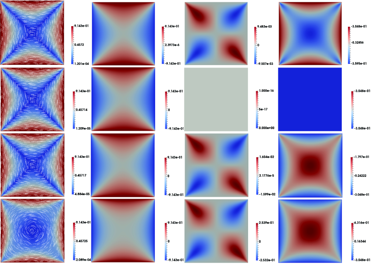
We investigate the effect of $\hat{L}_{2}$ on the $WORS$-profile, using asymptotic methods. The $WORS$ in the form of (12), given by the triplet $(q,0,-B/6C)$ at the fixed temperature $A=-B^{2}/3C$, where $q$ is a solution of the Allen-Cahn equation, as in canevari2017order. With the leading order approximation given by $(q,0,-B/6C)$, we expand $q_{1},q_{2},q_{3}$ in powers of $\hat{L}_{2}$ as follows:

	$\displaystyle q_{1}(x,y)$	$\displaystyle=q(x,y)+\hat{L}_{2}f(x,y)+\dots$		(35)
	$\displaystyle q_{2}(x,y)$	$\displaystyle=\hat{L}_{2}g(x,y)+\dots$
	$\displaystyle q_{3}(x,y)$	$\displaystyle=-\frac{B}{6C}+\hat{L}_{2}h(x,y)+\dots$

for some functions $f,g,h$ which vanish on the boundary.

For $\lambda$ small enough, one can show that the corrections $(f,g,h)$ are unique, $g\equiv 0$ on $\Omega$ and $f(x,y)=0$ on diagonals. Hence, for $\lambda$ small enough, the cross structure of the $WORS$ is lost mainly because of effects of $\hat{L}_{2}$ on the component $q_{3}$.

We work at the fixed temperature $A=-B^{2}/3C$ for all the following numerical results. We perform a parameter sweep of $\bar{\lambda}^{2}$, from $5$ to $500$, and find one of the symmetric solution branches constructed in Proposition VI.1, with various fixed $\hat{L}_{2}$. The solutions with $\bar{\lambda}^{2}=500$ are plotted in Fig. 12. When $\hat{L}_{2}=0$, we recover the familiar $WORS$ for all $\lambda>0$. When $-1<\hat{L}_{2}<0$, the solution exhibits a $+1$-defect at the square center, and we refer to it as the $Ring^{+}$ solution. When $\hat{L}_{2}$ is positive and moderate in value, we recover the $Ring^{+}$ solution branch and $q_{3}>-s_{+}/6$ at the square centre. When $\hat{L}_{2}$ is large enough, we discover a new symmetric solution which is approximately constant, $(q_{1},q_{2},q_{3})=(0,0,s_{+}/3)$, away from the square edges, as shown in the fourth row of Fig. 12 for $\hat{L}_{2}=10$. We refer to this novel solution as the Constant solution.

References

- [1] Friedrich Reinitzer. Beiträge zur kenntniss des cholesterins. Monatshefte für Chemie, 9(1):421–441, 1888.
- [2] Jan PF Lagerwall. An introduction to the physics of liquid crystals. Fluids, Colloids and Soft Materials: An. Introduction to Soft Matter Physics; Fernandez-Nieves, A., Puertas, AM, Eds, pages 307–340, 2016.
- [3] Georges Friedel. Les états mésomorphes de la matière. In Annales de physique, volume 9, pages 273–474, 1922.
- [4] Pierre Gilles de Gennes and J Prost. The Physics of Liquid Crystals, volume 83. Oxford university press, 1995.
- [5] Peter Palffy-Muhoray. Orientationally ordered soft matter: The diverse world of liquid crystals. Electronic-Liquid Crystal Communications (e-LC), 2007.
- [6] Birendra Bahadur. Liquid Crystal-Applications And Uses (Volume 1), volume 1. World scientific, 1990.
- [7] Jan PF Lagerwall and Giusy Scalia. A new era for liquid crystal research: Applications of liquid crystals in soft matter nano-, bio-and microtechnology. Current Applied Physics, 12(6):1387–1412, 2012.
- [8] VSR Jampani, RH Volpe, K Reguengo de Sousa, J Ferreira Machado, CM Yakacki, and JPF Lagerwall. Liquid crystal elastomer shell actuators with negative order parameter. Science advances, 5(4):eaaw2476, 2019.
- [9] Lars Onsager. The effects of shape on the interaction of colloidal particles. Annals of the New York Academy of Sciences, 51(4):627–659, 1949.
- [10] Wilhelm Maier and Alfred Saupe. Eine einfache molekulare theorie des nematischen kristallinflüssigen zustandes. Zeitschrift für Naturforschung A, 13(7):564–566, 1958.
- [11] J. L. Ericksen. Liquid crystals with variable degree of orientation. Arch. Rational Mech. Anal., 113(2):97–120, 1990.
- [12] CW Oseen. The theory of liquid crystals. Transactions of the Faraday Society, 29(140):883–899, 1933.
- [13] Apala Majumdar and Arghir Zarnescu. Landau-de Gennes theory of nematic liquid crystals: the Oseen-Frank limit and beyond. Archive for rational mechanics and analysis, 196(1):227–280, 2010.
- [14] Y. Han, J. Harris, L. Zhang, and A. Majumdar. Elastic anisotropy of nematic liquid crystals in the two-dimensional Landau–de Gennes model. arXiv preprint arXiv:2105.10253, 2021.
- [15] Apala Majumdar. Equilibrium order parameters of nematic liquid crystals in the landau-de gennes theory. European Journal of Applied Mathematics, 21(2):181–203, 2010.
- [16] Maurice Kléman. Defects in liquid crystals. Reports on Progress in Physics, 52(5):555, 1989.
- [17] Halim Kusumaatmaja and Apala Majumdar. Free energy pathways of a multistable liquid crystal device. Soft matter, 11(24):4809–4817, 2015.
- [18] J Cliff Jones. Defects, flexoelectricity and rf communications: the zbd story. Liquid Crystals, 44(12-13):2133–2160, 2017.
- [19] C Tsakonas, AJ Davidson, CV Brown, and Nigel J Mottram. Multistable alignment states in nematic liquid crystal filled wells. Applied physics letters, 90(11):111913, 2007.
- [20] Jong-Hyun Kim, Makoto Yoneya, and Hiroshi Yokoyama. Tristable nematic liquid-crystal device using micropatterned surface alignment. Nature, 420(6912):159–162, 2002.
- [21] Silvan Gantenbein, Kunal Masania, Wilhelm Woigk, Jens PW Sesseg, Theo A Tervoort, and André R Studart. Three-dimensional printing of hierarchical liquid-crystal-polymer structures. Nature, 561(7722):226–230, 2018.
- [22] Iain W Stewart. The static and dynamic continuum theory of liquid crystals: a mathematical introduction. Crc Press, 2019.
- [23] YC Han, A Majumdar, and L Zhang. A reduced study for nematic equilibria on two-dimensional polygons. SIAM Journal on Applied Mathematics, 80(4):1678–1703, 2020.
- [24] Lidong Fang, Apala Majumdar, and Lei Zhang. Surface, size and topological effects for some nematic equilibria on rectangular domains. Mathematics and Mechanics of Solids, 25(5):1101–1123, 2020.
- [25] YC Han, JY Yin, PW Zhang, A Majumdar, and L Zhang. Solution landscape of a reduced Landau–de Gennes model on a hexagon. Nonlinearity, 34(4), 2021.
- [26] Epifanio G Virga. Variational theories for liquid crystals, volume 8. CRC Press, 1995.
- [27] Fang Hua Lin and Chun Liu. Static and dynamic theories of liquid crystals. J. Partial Differential Equations, 14(4):289–330, 2001.
- [28] N. J. Mottram and C. Newton. Introduction to Q-tensor theory. Technical Report 10, Department of Mathematics, University of Strathclyde, 2004.
- [29] Henricus H Wensink. Polymeric nematics of associating rods: Phase behavior, chiral propagation, and elasticity. Macromolecules, 52(21):7994–8005, 2019.
- [30] Peter J Wojtowicz, Ping Sheng, and EB Priestley. Introduction to liquid crystals. Springer, 1975.
- [31] Chong Luo, Apala Majumdar, and Radek Erban. Multistability in planar liquid crystal wells. Physical Review E, 85(6):061702, 2012.
- [32] Dmitry Golovaty, José Alberto Montero, and Peter Sternberg. Dimension reduction for the Landau-de Gennes model in planar nematic thin films. Journal of Nonlinear Science, 25(6):1431–1451, 2015.
- [33] Y. C. Han, Y. C. Hu, P. W. Zhang, and L. Zhang. Transition pathways between defect patterns in confined nematic liquid crystals. Journal of Computational Physics, 396:1–11, 2019.
- [34] A Sonnet, A Kilian, and S Hess. Alignment tensor versus director: Description of defects in nematic liquid crystals. Physical Review E, 52(1):718, 1995.
- [35] Giacomo Canevari, Apala Majumdar, and Amy Spicer. Order reconstruction for nematics on squares and hexagons: A Landau-de Gennes study. SIAM Journal on Applied Mathematics, 77(1):267–293, 2017.
- [36] Yiwei Wang, Giacomo Canevari, and Apala Majumdar. Order reconstruction for nematics on squares with isotropic inclusions: A Landau-de Gennes study. SIAM Journal on Applied Mathematics, 79(4):1314–1340, 2019.
- [37] Samo Kralj and Apala Majumdar. Order reconstruction patterns in nematic liquid crystal wells. Proceedings of the Royal Society A: Mathematical, Physical and Engineering Sciences, 470(2169):20140276, 2014.
- [38] Alexander H Lewis, Ioana Garlea, José Alvarado, Oliver J Dammone, Peter D Howell, Apala Majumdar, Bela M Mulder, MP Lettinga, Gijsje H Koenderink, and Dirk GAL Aarts. Colloidal liquid crystals in rectangular confinement: theory and experiment. Soft Matter, 10(39):7865–7873, 2014.
- [39] Martin Robinson, Chong Luo, Patrick E Farrell, Radek Erban, and Apala Majumdar. From molecular to continuum modelling of bistable liquid crystal devices. Liquid Crystals, 44(14-15):2267–2284, 2017.
- [40] Giacomo Canevari, Joseph Harris, Apala Majumdar, and Yiwei Wang. The well order reconstruction solution for three-dimensional wells, in the Landau-de Gennes theory. arXiv preprint arXiv:1903.03873, 2019.
- [41] Fabrice Bethuel, Haïm Brezis, Frédéric Hélein, et al. Ginzburg-Landau Vortices, volume 13. Springer, 1994.
- [42] Michael A Brilleslyper, Michael J Dorff, Jane M McDougall, James S Rolf, Lisbeth E Schaubroek, Richard L Stankewitz, and Kenneth Stephenson. Explorations in complex analysis, volume 40. Mathematical Association of America, 2012.
- [43] Fabrice Bethuel, Haïm Brezis, and Frédéric Hélein. Asymptotics for the minimization of a Ginzburg-Landau functional. Calculus of Variations and Partial Differential Equations, 1(2):123–148, 1993.
- [44] Lidong Fang, Apala Majumdar, and Lei Zhang. Surface, size and topological effects for some nematic equilibria on rectangular domains. Mathematics and Mechanics of Solids, 25(5):1101–1123, 2020.
- [45] Patricia Bauman, Jinhae Park, and Daniel Phillips. Analysis of nematic liquid crystals with disclination lines. Archive for Rational Mechanics and Analysis, 205(3):795–826, 2012.
- [46] X. Lamy. Bifurcation analysis in a frustrated nematic cell. J. Nonlinear Sci., 24(6):1197–1230, 2014.
- [47] J. W. Milnor, M. Spivak, and R. Wells. Morse theory, volume 1. Princeton university press Princeton, 1969.
- [48] L. Zhang, W. Q. Ren, A. Samanta, and Q. Du. Recent developments in computational modelling of nucleation in phase transformations. NPJ Computational Materials, 2:16003, 2016.
- [49] Jianyuan Yin, Yiwei Wang, Jeff ZY Chen, Pingwen Zhang, and Lei Zhang. Construction of a pathway map on a complicated energy landscape. Physical review letters, 124(9):090601, 2020.
- [50] YC Han, J Harris, and A Majumdar. Tailored nematic and magnetization profiles on two-dimensional polygons. Physical Review E, 103(052702), 2021.
- [51] Ruma Rani Maity, Apala Majumdar, and Neela Nataraj. Discontinuous galerkin finite element methods for the landau–de gennes minimization problem of liquid crystals. IMA Journal of Numerical Analysis, 41(2):1130–1163, 2021.
- [52] Ruma Rani Maity, Apala Majumdar, and Neela Nataraj. Error analysis of nitsche’s and discontinuous galerkin methods of a reduced landau–de gennes problem. Computational Methods in Applied Mathematics, 21(1):179–209, 2021.
- [53] Wells GE Logg A, Mardal KA. Automated solution of differential equations by the finite element method: the FEniCS book, volume 84. Springer Science and Business Media, 2012.
- [54] JC Fabero, Alfredo Bautista, and Luis Casasús. An explicit finite differences scheme over hexagonal tessellation. Applied Mathematics Letters, 14(5):593–598, 2001.
- [55] Jianyuan Yin, Lei Zhang, and Pingwen Zhang. High-index optimization-based shrinking dimer method for finding high-index saddle points. SIAM Journal on Scientific Computing, 41(6):A3576–A3595, 2019.