Revisiting near the using analyticity and the left-cut structure
Abstract
Amplitudes of the form appear as sub-processes in the computation of the muon . We test a proposed theoretical modelling against very precise experimental measurements by the KLOE collaboration at . Starting from an exact parameter-free dispersive representation for the -wave satisfying QCD asymptotic constraints and Low’s soft photon theorem we derive, in an effective theory spirit, a two-channel Omnès integral representation which involves two subtraction parameters. The discontinuities along the left-hand cuts which, for timelike virtualities, extend both on the real axis and into the complex plane are saturated by the contributions from the light vector mesons. In the case of , we show that a very good fit of the KLOE data can be achieved with two real parameters, using a -matrix previously determined from scattering data. This indicates a good compatibility between the two data sets and confirms the validity of the -matrix. The resulting amplitude is also found to be compatible with the chiral soft pion theorem. Applications to the scalar form factors and to the resonance complex pole are presented.
1 Introduction
The discrepancy between the experimental determinations of the muon and its calculation within the Standard Model (e.g. [1]) has recently been confirmed by a new measurement [2]. Since the soft hadronic contribution to the has the largest error in the calculation it seems necessary to further investigate the theoretical descriptions of amplitudes involving light mesons together with real or virtual photons and to also further improve our knowledge of the interactions of these mesons among themselves and the properties of the associated light resonances.
We reconsider here the description of amplitudes of the form involving one real and one virtual photon. In the context of the , the channel is the most relevant one. It was considered in refs. [3, 4], also in the case of two virtual photons, using a method which applies when the energy of the system is much smaller than 1 GeV. Recently, a generalisation was performed [5], from which the contribution of the resonance to the muon was estimated. We develop here a similar approach, in the case of one virtual photon, which can be applied in an energy region of the system slightly larger than 1 GeV. We focus on the case where , and will test the method against the very precise measurements performed by the KLOE collaboration close to the meson peak [6] (earlier results can be found in [7, 8, 9, 10]). The amplitudes , have large resonant contributions induced by the scalar mesons , respectively. Initial interest in measuring such amplitudes was stimulated by the claim [11] that this would allow to clearly discriminate between models of these presumably exotic mesons (the [12] versus the molecule model [13, 14]) but some disagreements with this claim have been expressed (e.g. [15]). We refer to [16] for a review on this topic.
Our objective here is rather to probe both the quality of the description of the radiative amplitude which can be achieved and the properties of the -wave -matrix globally in the low/medium energy range. While the existence of a sharp scalar resonance coupling to both and channels was established long ago [17, 18] the detailed behaviour of the phase shifts is still controversial. The pattern which was established in lattice QCD simulations [19] at MeV may or may not extend down to the physical pion mass value, depending on the extrapolation model [20]. A very similar phase shift pattern was found to emerge in the meson-meson scattering model developed in ref. [21] which was applied to scattering in ref. [22] and found to describe reasonably well the data by the Belle collaboration [23]. However, the mass and width properties of the resonance in this model are not compatible with the PDG values. Moreover, a determination of the scattering matrix performed in ref. [24] using the same set of data, together with data on from [25] and from [26] obtained different results for the phase shifts and for the properties of the resonance.
Our approach is based on the general analyticity structure of the partial waves and the use of the Omnès method [27] (extended to several channels [28]) which ensures, by construction, that two-channel unitarity is exactly satisfied. In some previous work [11, 29, 30] the emphasis has been on a quick determination of the parameters, but the amplitude models eventually violate unitarity, which may introduce a bias in this determination. The amplitude models used in refs. [31, 32] based on a unitarisation of the leading order chiral expansion (uPT) do fulfil unitarity (the relation to our formalism is worked out in appendix A) but the underlying -matrix is possibly somewhat unrealistic (having e.g. no left-hand cuts).
We develop an Omnès-type representation for -waves which involves explicit integrations over the left-cut. When the virtuality is negative or vanishing, this left-cut has a simple structure, lying on the negative real axis, but this changes for timelike virtualities. In that case, the left-cut has several components extending in the complex plane [33]. The integrations have to be done carefully and we explain this in detail. One component of this left-cut eventually overlaps with part of the unitarity cut and turns around the threshold point. In addition the Born amplitude has a pole singularity which also lies on top of the unitarity cut. These singularities induce a deviation of the phase of the partial wave from the the elastic phase shift such that Watson’s theorem does not apply [34]. A further consequence concerns the Adler zero which, in the partial wave, is moved to an unphysical Riemann sheet.
This coupled-channel dispersive representation involves two real subtraction parameters. The presence of subtraction parameters is a necessary and unavoidable consequence of the effective-theory nature of dispersion relations and should not be omitted, they absorb required corrections to the higher energy parts of the integrations. The minimal number of subtractions is determined from the asymptotic bounds on the partial waves and the dynamical constraints which must be satisfied, like the exact soft photon zero in the present case [35]. Because of the very small number of undetermined parameters which are involved, the amplitudes , similarly to , are very good probes of the final-state interaction -matrix. We will show that a rather good fit of the KLOE data [6] on can be achieved with two fit parameters, using a -matrix previously determined from data [24]. We will also study how combining the two sets of data can help improve the determination of the -matrix and the properties of the resonance.
The plan of the paper is as follows. After recalling some general properties related to gauge invariance we discuss the origin of the cuts in the partial waves and the approximations to be used for evaluating the discontinuities, based on vector meson exchanges in crossed channels. Starting form a general, exact, dispersive representation for the partial waves of interest we derive a coupled-channel Omnès representation valid in the considered energy region. This representation involves two subtraction parameters and a number of integrals over both the unitarity cut and the left cuts. We then discuss the evaluation of the vector meson coupling constants which are needed (including their relative signs) using experimental inputs together with flavour, chiral and asymptotic constraints. After explaining how to accurately compute all the integrals over the complex contours we perform a detailed comparison with the experimental data and discuss some consequences.
2 General formalism
2.1 Tensor and helicity amplitudes
We first recall that amplitudes involving two real or virtual photons and two pseudo-scalar mesons can be derived from a correlation function involving two electromagnetic currents
| (1) |
Current conservation implies that the tensor must satisfy the two Ward identities
| (2) |
One can then expand over a basis of five independent tensors (e.g. [36]) satisfying (2) formed with the three independent momenta , and ,
| (3) |
We consider here more specifically the situation where one photon is real and the other is virtual,
| (4) |
In this case, the tensors , are not physically relevant.
The dependence as a function of the virtuality is expected to display large Breit-Wigner peaks associated with the light vector resonances ,,, such that
| (5) |
where describes the amplitude for the vector meson to decay into . We will consider here the situation where is close to the peak of the resonance i.e. , and focus on the construction of the amplitude , assuming that the background contributions from the the other vector resonances can be neglected or have been subtracted. In the sequel, the index will be dropped. This amplitude can be expanded in terms of the independent tensors as
| (6) |
where the functions , , are Lorentz scalars depending on the external masses and on the Mandelstam invariants , , ,
| (7) |
which satisfy . We can derive the helicity amplitudes by contracting the tensorial amplitude with the polarisation vectors of the photon and the meson
| (8) |
(with a conventional minus sign). The scattering angle is defined as the angle between and in the centre-of-mass system of the two pseudoscalar mesons (see fig. 1). The Mandelstam variables , are expressed as follows as a function of
| (9) |
where
| (10) |
with
| (11) |
The three independent helicity amplitudes, finally, can be written in terms of the three functions , , as
| (12) |

2.2 Partial waves and their singularities
We will designate the helicity amplitudes of interest as
| (13) |
The isospin amplitudes are related to the , ones by
| (14) |
and we consider here the coupled-channel system of the two -waves with
| (15) |
The angular integration can be expressed in terms of the -variable, e.g. for the amplitude
| (16) |
with
| (17) |
Let us first examine the singularities of the partial wave when and :
- 1)
Singularity when : When , the lower integration boundary in eq. (16) goes to since one has
(18) which leads to a singular behaviour of (see [37]). The behaviour of the amplitude in the regime when and is driven by the Regge trajectory which gives,
(19) with , . Using this in eq. (16) one obtains for the -wave near ,
(20) - 2)
Singularities when : When performing the -integration (16) with a fixed value of the energy one must pay attention to the cuts of the function in the variable. In the -channel, which we can write the lightest unitarity contributions are from isoscalar states which generates a cut in the variable lying on the real axis from to . Similarly, in the channel the lightest unitarity contributions are from isovector states. This generates a cut in the variable extending from to with . This cut can be shifted away from the real axis by appending an infinitesimal imaginary part to
(21) When is in the physical region, is real and one easily verifies that
(22) The integration path in eq. (16) therefore lies in between the two cuts without touching them for finite values of . The situation changes when is in the unphysical region where is imaginary. The path of integration must then be distorted to turn around the cut as illustrated in fig. 2. As a consequence, the partial wave diverges when approaches the threshold from below since the integral in eq. (16) remains finite while in the denominator vanishes. A similar divergence occurs when approaches the pseudo-threshold from above. The discontinuities of when moves across the points reflect the fact that crosses the cut of the partial-wave amplitude at these points. This cut will be described in more detail below.
The singularities of the partial waves when crosses the points affects the position of the Adler zero. The existence of an Adler zero in the chiral limit when the pion is soft, i.e. , implies that the physical helicity amplitude should have an Adler zero at , . The Adler zero is also present in the partial wave for small enough virtualities11 1 The condition for to be a smooth function in the whole range is that when . This is satisfied when , GeV2.. When increases the zero is no longer present in the first Riemann sheet.

2.3 Partial-wave dispersion relations
One can estimate the asymptotic behaviour of the amplitudes or when while (or ) remains finite, based on Regge theory. It is also possible to make estimates in the regime where all three Mandelstam variables go to infinity based on quark counting rules [38]. These arguments suggest that the partial waves and should remain bounded by asymptotically and should thus satisfy once-subtracted dispersion relations. These should be constrained to satisfy Low’s soft photon theorem [35],
| (23) |
where is the , projection of the pole contribution to . As we will review below (in sec. 3.4) the -wave amplitude has the following form
| (24) |
where, for real values of , the function is given by
| (25) |
The function is an analytic function of with a cut along the negative real axis,
| (26) |
The amplitude is thus also an analytic function of except for a cut on the negative axis and a pole at (which corresponds to the soft photon limit). It satisfies the following dispersive representation
| (27) |
with
| (28) |
The amplitudes are symmetric in the , variables due to -invariance. Singularities in the crossed channels , apart from the charged kaon pole , are induced by unitarity contributions from states: , . We will approximate these by the resonance contribution: . These cross-channel singularities generate a cut in the partial-wave amplitude, denoted as illustrated in fig. 5 below. This cut includes the negative real axis and also has a complex component.
The amplitudes are not symmetric in the variables ,. This leads to two different cuts in the partial waves which we will denote as and (see fig. 5). The cut corresponds to unitarity contributions in the -channel which has isospin i.e. they are generated from , , , intermediate states. We will approximate these by the and resonance contributions: . In the -channel the unitarity contributions have states ( , , , ) and will be approximated by the -meson contribution: . In addition to these left-hand (and complex) cuts the partial wave amplitudes have a unitarity right-hand cut on the positive real axis .
On must also check for the possible presence of an anomalous threshold. Anomalous thresholds occur when one of the endpoints of the left-hand cut requires a deformation of the unitarity cut [39] (see [40] for a review). This happens for amplitudes involving two virtual photons (e.g. , see [41, 4]). In our case, only one photon is virtual. With the , -channel exchanges which we have considered and the two-body channels included in the unitarity relation we have checked that no anomalous threshold gets generated when varying the virtuality .
Finally, taking the soft-photon constraints and the asymptotic bounds into account one can write the following dispersive integral representations for the partial waves , ,
| (29) |
and
| (30) |
with
| (31) |
The discontinuity along the real axis is defined as
| (32) |
Along the complex contour, the corresponding definition is given in terms of the parametric representation in eq. (105) below.
The dispersive integral representations given in eqs. (29) (30) can be considered as exact. In practice, one intends to estimate the partial-wave amplitudes in the energy region relevant for the decay i.e. . The dispersive equations (29) (30) must be used in an effective theory sense: one tries to perform accurate approximations to the integrands in a limited energy region e.g. while absorbing the remaining higher energy contributions into a finite number of low energy parameters. In this work, we implement the following approximations:
- a)
Along the left-hand and complex cuts we approximate the discontinuities by those of the light vector mesons (, , , ) and by the exchange contributions to the amplitudes,
(33) - b)
Along the right-hand cut we evaluate the discontinuity from the unitarity relations, including two channels
(34) where is the two-channel -wave -matrix with
(35) and
(36)
Using these approximations for the discontinuities in eqs. (29) (30) generates a closed set of coupled-channel Muskhelishvili equations [42]. The solutions of these equations will include subtraction parameters which account for the contributions of the higher energy regions in the dispersive integrals where the approximations made above are no longer valid.
2.4 Coupled-channel Omnès-Muskhelishvili representation
The fundamental ingredient for expressing the solutions of these equations is the matrix [42]. The matrix elements are defined to be real-analytic functions of , having a cut on the positive real axis and the discontinuity across this cut being given by
| (37) |
In order to write dispersion relations for the matrix elements we make the assumption that when . Other choices can obviously be made22 2 In non-relativistic scattering theory, for instance, the corresponding Jost matrix is defined such as to go to the identity when [43] but this one is convenient because it reproduces the asymptotic behaviour of scalar form-factors in QCD. The form factors are then related to the matrix elements by simple linear relations (see [44] and ref. [45] for the analogous case). Writing unsubtracted dispersion representations for the functions provides a relation between and the -wave -matrix in the form of a singular integral matrix equation
| (38) |
In general, this equation must be solved numerically but the determinant of can be expressed analytically in terms of the two phase shifts , ,
| (39) |
The phases are defined as continuous functions and the following asymptotic condition is imposed
| (40) |
where is the so-called Noether index [46, 42]. Taking ensures that eq. (38) has a unique solution with . One also sees from eq. (39) that the determinant of the Omnès matrix does not vanish (except at infinity) such that the inverse of is defined for all . We will use the (conventional [47]) notation for this inverse
| (41) |
As a simple consequence of the unitarity relations satisfied by the amplitudes , and by the matrix eqs. (34), (37), the two functions obtained by multiplying the amplitudes by the inverse of the Omnès matrix, have no discontinuity across ,
| (42) |
Based on this property, one can write various types of Omnès representations involving either only right-cut integrations [27] or only left-cut integrations [48] or both, which are exactly equivalent. We consider here a representation starting from the following two functions,
| (43) |
The terms subtracted from remove the soft-photon singularity at such that the functions , vanish at the soft photon point. These functions have both left and right-hand cuts.
When the matrix elements while the amplitudes , are expected to grow no faster than (see [24]). One can thus express , as twice-subtracted dispersion relations. It is natural to take as one of the subtraction points while the second one, , can be chosen arbitrarily. A variation of is compensated by a variation of the subtraction constants , . It is convenient to choose to lie on the real axis and away from the cuts, in the subthreshold region i.e. in the range . In this case we can expect the subtraction constants to be essentially real. The dispersive representations of , involve both left-cut and right-cut integrations. They can be written as follows, taking the soft photon constraints into account
| (44) |
where , are subtraction constants and the integrals along the cuts have the following form
| (45) |
Let us now express these integrals in more detail.
- 1)
Right-cut integrals: The discontinuities of the functions along the right-hand cut are driven by the singular parts of the Born amplitude. Their expressions are deduced from (43) using (42)
(46) Using the analyticity properties of the matrix elements these right-cut integrals can be calculated explicitly and one obtains
(47) with
(48) - 2)
Left-cut integrals: Along the left-hand cuts now, the discontinuities of the functions are proportional to those of the amplitudes , . Using the model defined in eq. (33), one can write the integrals in eq. (43) as a sum over five terms
(49) The integrals are associated with the left-cut discontinuity induced by the kaon pole, they read
(50) One remarks that the double pole at in the integrand does not cause any numerical difficulty when and that the integrals are real when is in the physical region (also assuming that the subtraction point is real and positive).
The transitions , or are all kinematically forbidden. In those cases, ignoring the width of the vector resonances is a good approximation. In the zero-width limit, the expressions for the integrals appearing in (49) are as follows, using the results from the next section on the discontinuities of the vector-exchange amplitudes,
(51) where
(52) and is a sign factor, (see sec. 4.2). The parameters , , are related to resonance chiral Lagrangian coupling constants introduced in the next section,
(53) In the case of the meson, the effect of the width must be taken into account because the transition is kinematically allowed. This can be done in a simple way, consistently with the analyticity properties, by replacing the -channel pole by a Källen-Lehmann dispersive representation [49, 50]. Denoting the zero-width limit of the integrals as with
(54) where
(55) one can express the finite-width result as an integral involving the corresponding Källen-Lehmann spectral function ,
(56) We will show in sec. 4.3 how to simplify this expression using integration by parts.
The radiative decay amplitudes have often been expressed in a form which involves the charged kaon (or charged pion) one-loop triangle function(e.g. [11, 51, 52, 53, 54, 55, 31, 56]), which seems different from the Omnès representations presented above. We show in appendix A that expressions in terms of the triangle loop function can indeed be derived from our dispersive representation for certain specific models of -matrices which, in particular, have no left-hand cut. Physically, of course, all the -matrix elements for scattering do have left-hand cuts (and a complex cut in the case of ) such that the Kaon-loop representation is not exactly valid.
3 Born and vector-exchange amplitudes
In this section we review the evaluation of the Born amplitude and that of the vector-exchange amplitudes based on a resonance chiral Lagrangian. The Born amplitude is proportional to the coupling constant, the magnitude of which can be evaluated from experiment. The vector meson exchange contributions to and involve the product of a radiative decay coupling, the magnitude of which can be determined from experiment, and a hadronic coupling. Among those, only the and couplings can be estimated from experiment. We can use flavour symmetry and large arguments in order to derive estimates for the other couplings which are needed. This will also allow us to relate the sign of the Born amplitude to those of the vector exchange amplitudes.
3.1 Resonance chiral Lagrangian and mixing angle
We start from the following resonance chiral Lagrangian [57]
| (57) |
with . We differ from ref. [57] in considering a nonet (rather than an octet) of vector mesons, which are encoded in a matrix with
| (58) |
The Lagrangian (57) is of leading order in the large and in the chiral expansions i.e. , . We consider only the couplings which are relevant to the amplitudes of interest here. In the terms proportional to we use the same notation as [58]. The pseudoscalar fields are encoded, as usual, in a unitary matrix and with . The external vector and axial-vector sources can be set to , , so that
| (59) |
where is the photon field. With these definitions we can express the matrix element of the electromagnetic current,
| (60) |
In order to get the correct pattern for the masses of the vector mesons we must add mass terms which break both the flavour and the nonet symmetries,
| (61) |
where is the quark mass matrix and the parameter is sub-leading in the large expansion i.e. . These flavour and nonet symmetry-breaking terms induce a mixing between the and the mesons, with a mixing angle , such that the matrices attached to the physical and mesons can be written as
| (62) |
with
| (63) |
where is the “ideal” mixing angle. We can first derive two relations between the Lagrangian parameters and the and meson masses and then, the masses of the and mesons are obtained by diagonalising the singlet-octet mass matrix. After a rotation by the ideal mixing angle this matrix reads
| (64) |
In this form, it is easy to see that the experimental fact that implies that . To leading order in , one obtains for the angle
| (65) |
This formula shows that , even though numerically small, is actually chirally enhanced because the denominator is . This provides some justification for neglecting further Lagrangian terms which break the nonet symmetry. The masses of the and mesons (i.e. the eigenvalues of ) are given by
| (66) |
to leading order in . This implies the mass relation
| (67) |
which is verified within 4%. This small discrepancy, however, gives rise to a significant relative uncertainty in the evaluation of . Using the mass gives while using the mass gives .
3.2 Signs of the coupling constants
One can derive useful information on the signs of the coupling constants by using asymptotic constraints on the form factors. Let us define the form-factor as follows
| (68) |
where . We have factored out the coupling such that the form factor must satisfy , which ensures that the amplitude becomes equal to when . Computing the form factor in the flavour symmetry limit from the Lagrangian (57) one obtains [58]
| (69) |
Requiring that the form factor goes to zero when goes to infinity gives
| (70) |
Combining this result with the relation
| (71) |
which can be derived from a similar asymptotic constraint on the axial form factor [57] one obtains
| (72) |
This relation fixes the relative signs between the vector-exchange amplitudes which are proportional to and the Born amplitude which is proportional to . Without loss of generality we can choose , and to be positive.
3.3 and coupling constants
We will need a set of and couplings which can be defined from the Lagrangians
| (73) |
The magnitude of the couplings which are needed can all be determined from the experimental values of the radiative decay widths,
| (74) |
The results are collected in table 1 which also shows the expressions of these couplings using the resonance chiral chiral Lagrangian (57) with the leading order nonet symmetry breaking terms (61). For the amplitudes which involve an meson we use a simple mixing description such that the matrix attached to the meson is
| (75) |
and take . These expressions allow us to determine the signs of the couplings as shown in the table.
| flavour | exp. (GeV | flavour | exp.(GeV | ||
|---|---|---|---|---|---|
.
Let us now consider the couplings. As is well known, one can estimate the two couplings , from the experimental values of the decay widths. The decay amplitude derived from the resonance chiral Lagrangian (57) can be written in the following form
| (76) |
with
| (77) |
where is the -meson propagator taking the width into account (see sec. 4.2). Imposing the following asymptotic constraint33 3 This can be justified by matching to the asymptotic behaviour in the Brodsky-Lepage regime[59]: , fixed. on
| (78) |
and using that when yields the following relation which determines the value of
| (79) |
The amplitude (76) then becomes identical to that of the original GSW model [60] and to the one obtained from effective Lagrangians implementing a hidden-gauge symmetry [61]. From the expression of the width which reads
| (80) |
with
| (81) |
one obtains the following values for the couplings
| (82) |
The value of is compatible with the result derived from the experimental measurements of the form factor in the region in ref [62]. The errors quoted in eq. (82) do not contain the uncertainties induced by the modelling. Varying from the value given by eq. (79) by 20% induces a variation of by 14% and a variation of by 8%. It must also be kept in mind that these simple modellings of the amplitudes and of the form factors do not correctly account for the unitarity relations and the related dispersive representations [63, 64, 65, 66]. We finally ascribe a 20% uncertainty to the values of and . Using these two inputs, together with the couplings as shown in the table one can determine the values of the parameters , and from a least-squares fit. This yields
| (83) |
One can then deduce estimates for the values of the couplings , and which are needed in order to evaluate all the relevant vector-exchange amplitudes, The corresponding numerical values of the effective couplings which appear in front of the partial-wave amplitudes (see (53) (55)) are given by
| (84) |

3.4 Born amplitude
The Born amplitude in (see fig. 3) can now be computed from the Lagrangian (57). Including the contributions proportional to the two couplings and gives
| (85) |
with
| (86) |
This contribution is suppressed because of the approximate relation . Actually, our Omnès representations use only the singular parts of the tree amplitudes, other contributions being absorbed into the subtraction constants. Terms like (86) which make a constant contribution to the -wave can thus be omitted. We can replace in eq. (85) using the relation with the coupling
| (87) |
The coupling can be determined from the decay width,
| (88) |
which gives,
| (89) |
recalling that was chosen to have a positive sign. The three independent Born helicity amplitudes deduced from eq. (85) read
| (90) |
The partial-wave amplitude is then easily obtained
| (91) |
where was given in eq. (25).


3.5 Vector-exchange amplitudes
We can now express the vector-exchange amplitudes (see fig. 4) in terms of the couplings listed in table 1. These amplitudes involve the following two combinations of the three independent tensors
| (92) |
The exchange contributions to read
| (93) |
and the contributions from , and exchanges to read
| (94) |
These expressions are derived in the zero-width limit. Finite width effects will be discussed in sec. 4.2.
The helicity amplitudes corresponding to eqs. (93), (94) are deduced using the relations (12) and the partial-wave amplitudes are then easily computed. The partial-wave projections can be expressed in terms of the following generic function
| (95) |
with
| (96) |
and
| (97) |
The expressions of the and -wave amplitudes associated with vector meson exchanges are given below in terms of the functions,
| (98) |
and
| (99) |
4 Integrations along the complex cuts
4.1 Parametric representations of the cuts
It is easy to check that the function vanishes in the limit , as it should. Concerning the singularities, has a pole at when the two masses , are different. The function has square-root singularities at but these are not present in because it is an even function of . The remaining singularity of is a cut generated by the log functions. This cut is given by the values of such that the argument of one of the log’s is a negative real number, that is,
| (100) |
Solving for as a function of provides the following parametric representation of the cut,
| (101) |
An important point is that the shape of the cut does not depend on the mass of the exchanged vector meson. Only the lower bound on the variable depends on this mass, see (100). The cut of the amplitudes has two components, denoted as and corresponding to eq. (101) with and respectively. The left-cut of the amplitudes, denoted as is given by eq. (101) with . The cuts lie on the real axis when or otherwise they are complex. One sees that goes to when . The function can be re-written as
| (102) |
which shows that goes to 0 when . We also note that in the kinematical configuration where the endpoints of the cut are located on top of the unitarity cut. This corresponds to the triangle diagram singularities interpreted in ref. [67].


4.2 Testing the dispersive representations on the vector-exchange amplitudes
We first consider the partial-wave projections of the vector-exchange amplitudes and discuss their dispersive representations as integrals over the complex cuts. This allows us to check the correctness and the numerical accuracy of such integrals before extending them to the complete Omnès representation of the -wave.
The generic function which appears in the expressions of the -waves (see (95)) must satisfy the following Cauchy representation as an integral over the cut ,
| (103) |
with
| (104) |
taking into account the asymptotic behaviour, the pole44 4 As discussed in sec. 2.2 the singularity at in the full amplitude is weaker than a pole. at and the cut. The discontinuity across the cut is defined as follows
| (105) |
(where ). Using the explicit form of (eq. (95)) the discontinuity reads
| (106) |
where , depending on which one of the two log functions in generates the discontinuity. The integrations along the cut are expressed as follows, using the parametric representations
| (107) |
Fig. 5 illustrates the three different cuts , , which are involved and shows the regions where the sign factor in the discontinuity (106) is or in different colour. For the sign change occurs when the parameter and for when . Along the cut there are several sign changes which are indicated in table 2.
These three cuts include the negative real axis , as we have seen, and a complex component. In addition, the cuts extend along the positive real axis. These cuts can be shifted away from the unitarity cut by appending an infinitesimally small positive imaginary part to . Nevertheless, the cut crosses the real axis at the two points . When the energy crosses one of these points the discontinuity of the partial wave exhibits a divergence induced by the factor . This is in accordance with the discussion in sec. 2.2 on the path of integration for performing the partial-wave projection when is in the range .
Vector mesons are resonances and thus have a finite width. The width can be simply taken into account, in a way compatible with analyticity properties, by replacing the pole in the or variable in the tensorial vector-exchange amplitudes (93) (94) by a dispersive Källen-Lehmann [49, 50] representation
| (108) |
where in the case of the . We will assume that the spectral function satisfies the normalisation condition
| (109) |
which ensures that the propagator goes as when goes to infinity. In the case of the meson, for instance, we will use the following model for the spectral function55 5 This model differs from the one used in ref. [68] by a factor , which gives rise to somewhat simpler formulae.
| (110) |
where is proportional to the physical width
| (111) |
and is adjusted such that eq. (109) is satisfied. It is easy to see that the model (110) satisfies the condition that should tend to a function when the width goes to zero,
| (112) |
Using the finite width propagators (108), the vector-exchange partial-wave amplitudes, get expressed as integrals over , e.g.
| (113) |
The corresponding dispersive representations have the same form as eq. (103) in which the functions are expressed as double integrals,
| (114) |
These expressions can be simplified using integration by parts. Let us introduce the following two integrals of ,
| (115) |
which can be computed analytically using the model (110) (see appendix B). Integrating by parts, the functions get expressed in the following way in terms of and
| (116) |
which involves a single integration. The two terms involving are boundary contributions which will be detailed below. A remark is in order here: one sees from eq. (101) that , both vanish when . This generates a potentially highly singular term in the integral of eq. (116). This problem only affects the contour since, in this case, which lies within the range of integration. The functions , were chosen such as to vanish when (see (115)) and this removes completely these singularities in the -integral (116). The singular integrations are now contained in the two functions ,
| (117) |
They can be evaluated analytically in terms of the function , see (96)
| (118) |

4.3 Omnès integrations with a finite resonance width
Let us now return to the Omnès representations and reconsider the left-cut integrals , which were given in eq. (56) in the form of double integrals. The discussion in the preceding section can be easily adapted to derive expressions in the form of single integrals which are easy and fast to compute. One obtains,
| (119) |
where parametrise the contour and the functions are given by
| (120) |
These integrals must be computed numerically. When is in the physical range of the decay, , the numerical integration can be performed in a way which avoids the singularities at and by deforming the contour. Taking into account the exact cancellations in the regions of overlapping branches which have a different sign factor (see fig. 5) the contour can be deformed into a) the segment on the real axis (note that ), b) the four segments starting from and joining and c) the negative real axis. This deformed contour, showing the directions of integrations, is illustrated in fig. 6.
4.4 Recovering the Adler zero
The component of the complex cut in the partial wave which is induced by the meson exchange (and more generally by -channel exchanges) is responsible for the disappearance of the Adler zero, as was mentioned above. Indeed, this cut crosses the real axis at the two points and and this causes a divergence of the partial wave when approaches from below or from above. It is possible to recover the Adler zero by considering an analytical continuation of the amplitude to an unphysical Riemann sheet which we will call the Riemann sheet. Let us illustrate this in the case of the simple -exchange amplitude . The Riemann sheet extension is defined such as to match continuously with upon crossing the portion of the cut which extends from to . In the zero-width limit the two functions are simply related by
| (121) |
This formula is easily generalised to the case of a finite width using the integral representation of the amplitude and one finds
| (122) |
where the , are integrals of the spectral function which vanish at (see (160)). These -exchange partial-wave amplitudes are illustrated in fig. 7 which shows that the B-sheet extension displays an Adler zero close to .

5 Comparison with experiment
Given a -matrix satisfying two-channel unitarity and appropriate asymptotic conditions the -matrix (and its inverse ) can be determined numerically in a unique way. It is then only necessary to compute the left-cut integrals which appear in eqs. (44) and one obtains an expression for the two -wave decay amplitudes , in terms of two parameters , . An important check of the numerical implementation (which we have performed) is to verify that the discontinuities of the obtained solutions for , across the unitarity cut are exactly given by the unitarity equations (34).
In the numerical results presented below we use the two-channel -matrix model introduced in ref. [44]. In this model, two-channel unitarity is implemented using a -matrix approach. The form of this -matrix is recalled in appendix C: it is constrained such that the low-energy expansion of the corresponding -matrix matches with the chiral expansion (PT) up to NLO and it involves six phenomenological parameters. Determinations of these parameters were obtained in ref. [24] by performing fits to experimental measurements of , differential cross sections in an energy range GeV (a set of 688 data points was used). These fits are based on Omnès representations of the -wave amplitudes, exactly analogous to eqs. (43), (44) which depend on two subtraction parameters in addition to the -matrix parameters. Two different sets of -matrix parameters were actually found in the fits, giving approximately similar minimum values. One of these sets gives rise to a “narrow” resonance and has some unphysical features, it will not be considered here.
5.1 Left-cut and right-cut integrals


Let us now re-write the expressions of the -wave amplitudes in the Omnès-dispersive approach
| (123) |
in which we have defined to be the part of the the amplitude which vanishes at the soft photon point i.e.
| (124) |
The expressions of the four integrals , were given in eqs. (47) (48), (49), (51). The integrals are shown in fig. 8 along with the various vector meson contributions to the left-cut integrals . The contributions from the are enhanced by the fact that the effective coupling is one order of magnitude larger than the other couplings (see eq. (84)). The integrands of are proportional to the matrix elements , of the matrix (eqs. (51), (54)). At one has , and in the important integration region GeV2 the off diagonal matrix elements are suppressed in magnitude by roughly a factor of five as compared to the diagonal ones . This explains e.g. why , . A priori, one would expect the right-cut integrals to be dominant over the left-cut ones since they are induced by the diverging part of the Born amplitude. This turns out to be true in the case of the integrals as can be seen from fig. 8 (top). In the case of the integrals, however, one sees from the figure that is larger than the real part of .
5.2 Detailed comparison with KLOE results
In the physical decay region, the helicity amplitudes are dominated by the -wave. The amplitudes are approximated by the tree-level vector-exchange contributions. We have also made an estimate of the amplitude induced by the tensor meson exchange in the -channel (, see appendix D). This contribution turns out to be essentially negligible in the physical region. Using these amplitudes, the differential decay width of the mode as a function of the invariant mass squared can be expressed as follows in terms of the three independent helicity amplitudes
| (125) |
where are tree-level vector-exchange amplitudes with . We will compare the results from this theoretical model with the experimental measurements of the single differential decay width performed by the KLOE collaboration [6]. They are presented in table 5 of ref. [6] in the form of 49 data points which have been corrected from the background and the energy resolution effects. We will not include the last two points in the (see the discussion below). The is then computed from the following formula,
| (126) |
where is the error on the data point, MeV is the size of the energy bins, is the total width of the (we take MeV and the value of the photon virtuality MeV as in ref. [6]).
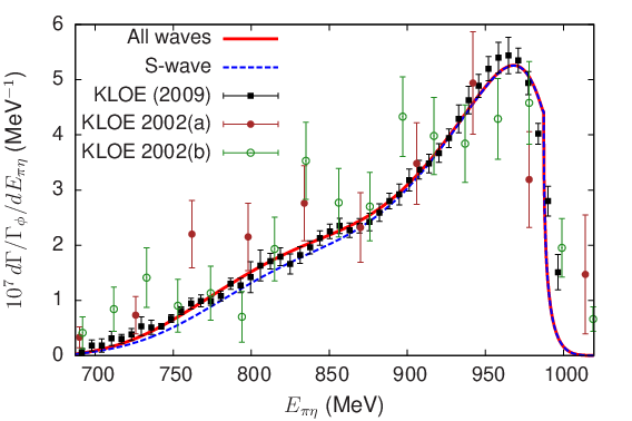
The determination of the -matrix parameters performed in ref. [24] is based on a dispersive Omnès description of the amplitudes involving two subtractions parameters. One of these was fixed by assuming a given position of the Adler zero in the -wave amplitude. Using the -matrix which corresponds to in the computation of the decay amplitudes and fitting the two parameters , to the KLOE data on gets . Taking a slightly larger value for the amplitude Adler zero:66 6 This value gives a somewhat better description of the data: using 688 data points (instead of ) and also a better description of the decay width distribution (see fig.10 in ref. [24] ) gives a -matrix which provides an even better fit to the decay data with and the values of , are
| (127) |
The ability to reproduce the decay data in the whole physical energy region with only two fit parameters77 7 For comparison, the fits performed in ref. [6] used either 5 parameters (KL model [11, 29]) or 7 parameters (NS model [30]) indicates a good compatibility between these data and the scattering data concerning the final-state rescattering -matrix.


The differential decay width corresponding to this fit is displayed in fig. 9 showing separately the contribution of the -wave. One sees a small but visible contribution from the higher waves in the energy region below 900 MeV. This contribution is dominated by the amplitude which is allowed for when . The two -wave amplitudes and obtained from this fit are plotted in fig. 10 and compared with the tree-level vector-exchange amplitudes. The amplitude is seen to qualitatively agree in size with the sum of the exchange and the regular part of the Born amplitude for energies below 0.8 . In contrast, the behaviour of the amplitude is dominated by the rescattering mechanism even at low energy. In the energy region below the threshold the Riemann sheet extension is shown (see sec. 4.4), which is expected to display an Adler zero . The figure shows that this is indeed the case. The central value of this zero is located at and its position varies in the range when varying the input values of the coupling constants which control the left-hand cut discontinuities. These features indicate that the fitted values of the two parameters , have a physically reasonable size.
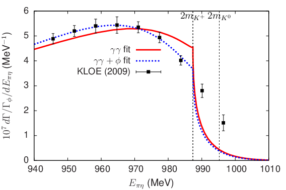
5.3 Combined and decay fits
We have seen that the -matrix determined from data is compatible with the decay data from KLOE. It is interesting to study how the -matrix parameters would be modified if the two data sets were combined. We have performed such a fit in which we have increased the weight of the decay data by a factor of two. In this way, the following total values are obtained,
| (128) |
showing a significant improvement in the data . At the same time the value of the data remains acceptable. For comparison, the fit including only data (with ) gives
| (129) |
The differential decay width in the two fits differ essentially in the higher energy region MeV. This is illustrated in fig. 11 which also shows the location of the , thresholds. One observes, in particular, a significant improvement on the last two points below the threshold (points 46 and 47) in the combined fit. However, the two points which are above (points 48 and 49) are not well described in either one of the fits. One observes that the energy of the point 48 is located in between the and the thresholds. It is possible that the discrepancy could be explained by isospin breaking effects which were predicted to be enhanced in this energy region [69]. In our model, isospin symmetry is assumed, and we have taken for the kaon mass in order to have the correct mass in the Born amplitude. Because of the importance of the Born amplitude in the rescattering dynamics it seems plausible that the cusp at the threshold should be significantly more pronounced than the one at the threshold. A complete treatment of isospin breaking effects is difficult since they induce couplings between the channels considered here and as well as channels. One must then use a six-channel -matrix and it is clearly not possible to determine all the -matrix elements in a model independent way. An example of a plausible modelling has been proposed e.g. in ref. [70].
On the experimental side, a clear observation of a two-particle threshold effect requires a very good energy resolution (for an example, see ref. [71]). The data points tabulated in ref. [6] are obtained after implementing a procedure for unfolding the energy resolution effects and subtracting the background. It is possible that this procedure becomes somewhat inaccurate near the tip of the Dalitz plot region.
Details of the numerical values of the -matrix parameters corresponding to different fits are given in appendix C. Fig. 12 shows the phase shifts and inelasticity parameter of the -matrix corresponding to two different fits. We observe that in these determinations the phase shift increases above the threshold while decreases. This pattern differs from the one found in the lattice QCD simulation [19].


5.4 complex pole and couplings
In the determinations of the two-channel -matrix performed in ref. [24] based on analysing scattering data, the resonance was always found to correspond to a pole of the -matrix located on the second Riemann sheet. No pole was found on the third or fourth Riemann sheet with a real part close to 1 . We recall the formulae which define the second sheet extension of the -matrix elements (see e.g. [40])
| (130) |
with
| (131) |
It is indeed easy to verify that the matrix elements satisfy the continuity equation across the cut
| (132) |
Simple definitions of the coupling constants can be associated with residues of the -matrix poles,
| (133) |
A formal definition of the width can be associated with the coupling ,
| (134) |
The coupling to , which is often quoted, is related to by
| (135) |
The magnitude of the couplings , as defined above should be approximately equal to those defined in refs. [11, 30].
The analytic extensions of the radiative decay -wave amplitudes to the 2nd Riemann sheet are defined as
| (136) |
which shows that they should display an pole. A coupling constant can be defined from the residue
| (137) |
This definition (which takes into account the presence of the nearby soft photon zero) matches to the one introduced in ref. [30].
The central values of the mass, width and couplings, corresponding to several fits are collected in table 3. The last column corresponds to a fit which combines the data and the data. In this fit, the mass is somewhat smaller as well as the coupling . As discussed in [24] an important source of uncertainty is generated by the “fixed” parameters in the -matrix, mainly the couplings and the ratio (see eqs. (171) (172)), as well as the value of the Adler zero in the amplitude. We have performed fits in which these parameters are varied around their central values in the same way as in [24] except for which we vary here in the range . As a result of this, we would quote the following determination of the mass/width from these data
| (138) |
and for the couplings
| (139) |
| fit | fit | fit | |
|---|---|---|---|
| (MeV) | 1000.6 | 1002.8 | 988.8 |
| (MeV) | 71.1 | 79.1 | 75.6 |
| (GeV) | 2.14 | 2.35 | 2.07 |
| (GeV) | 2.85 | 2.89 | 2.74 |
| (GeV-1) | 3.26 | 3.21 | 1.96 |


5.5 Scalar form factors
As already mentioned, the and scalar form factors are linearly related to the Omnès matrix elements which have been probed by the and the processes. In view of their applications to decays, it is convenient to define the scalar form factors from the matrix elements of the charged scalar current as
| (140) |
where and is the chiral coupling proportional to the quark condensate [72]. In a minimal construction, the form factors are related to the Omnès matrix simply by
| (141) |
(the minus sign being caused by ). At leading chiral order, the values at are given by
| (142) |
Expressions for the NLO corrections can be found e.g. in [44, 73]. Using the determination BE14 [74] for the chiral coupling constants (as used also here for the -matrix) one finds for the central values
| (143) |
Other chiral constraints that one might consider concern the scalar radii
| (144) |
which are not difficult to compute at order (see [44]). Using the BE14 value for the coupling , , one gets
| (145) |
The minimal dispersive model gives a result which is too small by 50% for the radius and too large by 40% for the one as compared to the values. While these differences can be ascribed, in part, to higher order corrections, it seems interesting to consider a non-minimal dispersive model in which one enforces exactly the values for both and . This is easily achieved by replacing in eq. (141) by linear functions of , , and adjusting the slope parameters . Fig. 13 shows results for the real and imaginary parts of the form factor in the minimal dispersive model using either LO or NLO values for and the result from the non-minimal model. Differences between the models remain rather small in the region of the resonance which is important for the decay. Our results are rather similar to those presented recently in ref. [73] but differ somewhat from ref. [75].
6 Summary and conclusions
We have re-examined the radiative decay amplitudes based on coupled-channel Omnès-type dispersive representations for the -waves, which seems not to have been done previously. By construction, these amplitudes have the correct analytic structure, with a left-hand cut having several components in addition to the unitarity cut, and the representation involves explicit integrations along these cuts. The discontinuities across the left-hand cut components were assumed to be dominated by the contributions from the light vector-meson resonance exchanges. The coupling constants which are needed can be determined approximately (including the relative signs) by combining experimental inputs with flavour and chiral symmetry arguments. This approach, which uses only the discontinuities of the vector-exchange amplitudes has the advantage of being insensitive to the off-shell behaviour of the resonance propagators (polynomial ambiguities, form factors) and allows to take into account the effects of the resonance widths in a numerically fast way.
The kaon exchange Born contribution to the amplitude plays an important role in the dynamics, as is well known, because it carries a pole when . It proved convenient to split this amplitude into a singular part and a regular part (which vanishes in the soft photon limit). The integrals involving the first part can be computed analytically in terms of matrix elements of the matrix. In practice, we describe the scattering using a two-channel unitary -matrix model proposed in [44], which has both left and right-hand cuts, and involves six phenomenological parameters. The corresponding (and ) matrices are computed numerically by solving a set of Muskhelishvili integral equations. In some previous work an apparently different representation was used (e.g. [11, 51, 52, 53, 54, 55, 31] ) which involves a one-loop triangle function and the -matrix itself. As shown in appendix A this representation holds only for restricted classes of -matrices which, in particular, have no left-hand cuts.
We have shown that a rather good description of the experimental data on can be obtained fitting only two subtraction parameters, while using in the -matrix a set of parameters determined previously from photon-photon scattering data. The fitted values of the two subtraction parameters were shown to be physically reasonable, such that the amplitude displays an Adler zero and the amplitude is dominated by the sum of the -exchange and the regular part of the -exchange amplitudes at low energy.
These results seem to confirm the validity of the two-channel -matrix model and the corresponding matrix. As an application, we give results for the and the scalar form factors (which are simply related to the matrix), they were shown to be well determined in the region of the resonance using chiral constraints at . The form factor is measurable, in principle, from the decay mode. Finally, we give some results on the complex pole, performing combined fits of data and radiative decay data.
Acknowledgements:
This work is supported by the European Union’s Horizon2020 research
and innovation programme (HADRON-2020) under the Grant Agreement n∘
824093.
Appendix A Relation between the Omnès and the kaon-loop representations
In this appendix we show that the Omnès representations for the amplitudes can be recast, for certain classes of -matrices, in a form which involves one-loop triangle functions. The kaon loop function, in particular, can be written in dispersive form as follows88 8 Analytical expressions can be found in refs. [11, 53]
| (146) |
Let us illustrate this in the case of the -matrices based on unitarised PT used in refs. [55, 31]. In these models the -matrices have no left-hand cut and the and matrices can be expressed explicitly as follows
| (147) |
where is the chiral -matrix and are one-loop functions which satisfy
| (148) |
In the Omnès representations we had separated the Born amplitude into a singular and a regular part
| (149) |
we can first express the right-cut integrals as
| (150) |
using the unitarity relation for the matrix elements
| (151) |
where the first equality is general and the second one follows from (147). The fact that are linear functions of is the key to the simplification. Indeed, we can express the Born left-cut integrals using a dispersive representation for the product (which remains finite when ) obtaining
| (152) |
Then, replacing with (151) and adding the two integrals one gets
| (153) |
We can then choose the subtraction point such that is a constant, which effectively pulls out from the integral. The remaining integral is equal to the kaon loop function . Finally, one arrives at the following form for the two amplitudes,
| (154) |
using that in this model. The integrals associated with meson exchanges e.g. in the Omnès representation can be similarly re-expressed in terms of simple triangle loop functions using eq. (151) which allows one to recover the formulae of ref. [32].
Appendix B -meson spectral function
Integrals involving the spectral function which describe the width of the meson, in particular , (eqs. (115)), are easily computed in the model given by eq. (110) by writing the denominator of , which is a cubic polynomial, as a product of three factors,
| (155) |
where is a real root and are complex conjugated. These roots must be computed numerically. The integrals of interest involve the following functions
| (156) |
For instance, one has
| (157) |
with
| (158) |
Taking the limit , one can determine from the normalisation condition (109) which yields
| (159) |
We can express in a similar way the following two integrals,
| (160) |
as
| (161) |
with
| (162) |
and
| (163) |
with
| (164) |
The integrals , introduced in eq. (115) are simply related to , ,
| (165) |
Finally, using this model, the propagator of the meson (eq. (108)) is expressed as a sum of four terms
| (166) |
Appendix C -matrix parametrisation
We briefly recall below the parametrisation of the two-channel (, ) -wave scattering amplitudes introduced in ref. [44]. The matrix is expressed in terms of a symmetric -matrix,
| (167) |
Two-channel unitarity is satisfied, as is well known, provided that the -matrix elements are real in the physical region and the -matrix satisfies
| (168) |
We use a -matrix which involves four phenomenological parameters
| (169) |
where are one-loop functions as defined in ref. [72], which satisfy and . The parameters , are real and assumed to be of chiral order .
The -matrix is written as a sum of three terms of increasing chiral order in which the terms of order and are determined by matching to the chiral expansion of the -matrix i.e.
| (170) |
where is the part of . The chiral expansions of up to NLO were first derived in [76] and in [77, 78]. The matching can be performed exactly for the matrix elements , but only approximately for in order to have real. The matrix elements depend on the Gasser-Leutwyler [72] coupling constants . In this work, their values were taken from table 3 of ref. [74] (BE14 set). The third term, , implements a -matrix pole
| (171) |
where and are phenomenological parameters while the form of is derived from a resonance chiral Lagrangian[79]
| (172) |
The central values of , were taken as
| (173) |
The form described above is used in a limited energy region with GeV. The -matrix must also be defined for in order to solve for the matrix. In this region, a simple interpolation of the two phase shifts (such that the sum goes to at infinity) and of the inelasticity (going to 1 at infinity) is implemented. We collect the numerical values of the sets of parameters corresponding to the fits described in sec. 5.4 in table 4 below.
| fit | fit | fit | |
|---|---|---|---|
| 0.996820807 | 0.984091282 | 1.0386891 | |
| -0.494739205 | -0.495522797 | -0.48956928 | |
| (GeV-1) | -4.14119816 | -3.78536367 | -4.5487204 |
| (GeV-1) | -0.185484648 | -0.120648287 | -0.16840835 |
| (GeV) | 0.899005413 | 0.910190940 | 0.88816762 |
| 1.06326795 | 1.07898855 | 1.0276550 |
Appendix D Estimate of the contribution
The contributions to the helicity amplitudes induced by the tensor resonance, i.e. have the following form,
| (174) |
where the constant is proportional to the product of the and couplings. Unfortunately, there is no experimental information on decay. It is possible to get a qualitative estimate of the coupling, relating it to the known coupling, using vector meson dominance ideas, following ref. [80]. This gives
| (175) |
where the coupling constants , , defined in [24], have the values
| (176) |
According to this estimate, one finds that the contribution from the resonance is rather small as compared to the vector-exchange contributions. For instance, at , defining the ratios one obtains
| (177) |
References
- [1] F. Jegerlehner, A. Nyffeler, Phys.Rept. 477, 1 (2009), 0902.3360
- [2] B. Abi et al. (Muon g-2), Phys. Rev. Lett. 126(14), 141801 (2021), 2104.03281
- [3] G. Colangelo, M. Hoferichter, M. Procura, P. Stoffer, JHEP 04, 161 (2017), 1702.07347
- [4] M. Hoferichter, P. Stoffer, JHEP 07, 073 (2019), 1905.13198
- [5] I. Danilkin, M. Hoferichter, P. Stoffer, Phys. Lett. B 820, 136502 (2021), 2105.01666
- [6] F. Ambrosino et al. (KLOE Collaboration), Phys.Lett. B681, 5 (2009), 0904.2539
- [7] A. Aloisio et al. (KLOE Collaboration), Phys.Lett. B536, 209 (2002), hep-ex/0204012
- [8] M. Achasov, S. Baru, K. Beloborodov, A. Berdyugin, A. Bozhenok et al., Phys.Lett. B479, 53 (2000), hep-ex/0003031
- [9] R.R. Akhmetshin et al. (CMD-2), Phys. Lett. B 462, 380 (1999), hep-ex/9907006
- [10] M.N. Achasov et al., Phys. Lett. B 438, 441 (1998), hep-ex/9809010
- [11] N. Achasov, V. Ivanchenko, Nucl. Phys. B 315, 465 (1989)
- [12] R.L. Jaffe, Phys. Rev. D 15, 267 (1977)
- [13] J.D. Weinstein, N. Isgur, Phys. Rev. Lett. 48, 659 (1982)
- [14] J.D. Weinstein, N. Isgur, Phys. Rev. D 27, 588 (1983)
- [15] Y.S. Kalashnikova, A.E. Kudryavtsev, A.V. Nefediev, C. Hanhart, J. Haidenbauer, Eur. Phys. J. A 24, 437 (2005), hep-ph/0412340
- [16] E. Klempt, A. Zaitsev, Phys.Rept. 454, 1 (2007), 0708.4016
- [17] A. Astier, L. Montanet, M. Baubillier, J. Duboc, Phys.Lett. B25, 294 (1967)
- [18] R. Ammar, R. Davis, W. Kropac, J. Mott, D. Slate, B. Werner, M. Derrick, T. Fields, F. Schweingruber, Phys. Rev. Lett. 21, 1832 (1968)
- [19] J.J. Dudek, R.G. Edwards, D.J. Wilson (Hadron Spectrum), Phys. Rev. D93(9), 094506 (2016), 1602.05122
- [20] Z.H. Guo, L. Liu, U.G. Meißner, J.A. Oller, A. Rusetsky, Phys. Rev. D95(5), 054004 (2017), 1609.08096
- [21] I.V. Danilkin, L.I.R. Gil, M.F.M. Lutz, Phys. Lett. B703, 504 (2011), 1106.2230
- [22] I. Danilkin, O. Deineka, M. Vanderhaeghen, Phys. Rev. D96(11), 114018 (2017), 1709.08595
- [23] S. Uehara et al. (Belle), Phys.Rev. D80, 032001 (2009), 0906.1464
- [24] J. Lu, B. Moussallam, Eur. Phys. J. C 80(5), 436 (2020), 2002.04441
- [25] S. Uehara et al. (Belle), PTEP 2013(12), 123C01 (2013), 1307.7457
- [26] H. Albrecht et al. (ARGUS), Z. Phys. C48, 183 (1990)
- [27] R. Omnès, Nuovo Cim. 8, 316 (1958)
- [28] J.D. Bjorken, Phys. Rev. Lett. 4, 473 (1960)
- [29] N.N. Achasov, A.V. Kiselev, Phys. Rev. D 68, 014006 (2003), hep-ph/0212153
- [30] G. Isidori, L. Maiani, M. Nicolaci, S. Pacetti, JHEP 0605, 049 (2006), hep-ph/0603241
- [31] E. Marco, S. Hirenzaki, E. Oset, H. Toki, Phys. Lett. B 470, 20 (1999), hep-ph/9903217
- [32] J. Palomar, L. Roca, E. Oset, M. Vicente Vacas, Nucl. Phys. A 729, 743 (2003), hep-ph/0306249
- [33] J. Kennedy, T.D. Spearman, Phys. Rev. 126, 1596 (1962), https://link.aps.org/doi/10.1103/PhysRev.126.1596
- [34] M.J. Creutz, M.B. Einhorn, Phys.Rev. D1, 2537 (1970)
- [35] F. Low, Phys.Rev. 110, 974 (1958)
- [36] W.A. Bardeen, W.K. Tung, Phys. Rev. 173, 1423 (1968), [Erratum: Phys.Rev.D 4, 3229–3229 (1971)]
- [37] H. Jakob, F. Steiner, Z. Phys. 228, 353 (1969)
- [38] S.J. Brodsky, G.P. Lepage, Phys. Rev. D24, 1808 (1981)
- [39] S. Mandelstam, Phys.Rev.Lett. 4, 84 (1960)
- [40] G. Barton, Introduction to dispersion techniques in field theory, Lecture notes and supplements in physics (W.A. Benjamin, New York, 1965)
- [41] M. Hoferichter, G. Colangelo, M. Procura, P. Stoffer (2013), 1309.6877
- [42] N.L. Muskhelishvili, Singular Integral Equations (P. Noordhof, Groningen, 1953)
- [43] R. Newton, Scattering Theory of Waves and Particles, Dover Books on Physics (Dover Publications, 2002), ISBN 9780486425351
- [44] M. Albaladejo, B. Moussallam, Eur. Phys. J. C 75(10), 488 (2015), 1507.04526
- [45] J.F. Donoghue, J. Gasser, H. Leutwyler, Nucl.Phys. B343, 341 (1990)
- [46] F. Noether, Math. Ann. 82, 42 (1921)
- [47] G.F. Chew, S. Mandelstam, Phys. Rev. 119, 467 (1960)
- [48] W.R. Frazer, J.R. Fulco, Phys. Rev. Lett. 2, 365 (1959)
- [49] G. Källen, Helv. Phys. Acta 25, 417 (1952)
- [50] H. Lehmann, Nuovo Cim. 11, 342 (1954)
- [51] S. Nussinov, T.N. Truong, Phys. Rev. Lett. 63, 1349 (1989), [Erratum: Phys. Rev. Lett.63,2002(1989)]
- [52] J.L. Lucio Martinez, J. Pestieau, Phys. Rev. D 42, 3253 (1990)
- [53] F. Close, N. Isgur, S. Kumano, Nucl. Phys. B 389, 513 (1993), hep-ph/9301253
- [54] A. Bramon, A. Grau, G. Pancheri, Phys. Lett. B 289, 97 (1992)
- [55] J.A. Oller, Phys. Lett. B 426, 7 (1998), hep-ph/9803214
- [56] A. Bramon, R. Escribano, J.L. Lucio M., M. Napsuciale, G. Pancheri, Phys. Lett. B 494, 221 (2000), hep-ph/0008188
- [57] G. Ecker, J. Gasser, H. Leutwyler, A. Pich, E. de Rafael, Phys. Lett. B 223, 425 (1989)
- [58] J. Prades, Z. Phys. C 63, 491 (1994), [Erratum: Z.Phys.C 11, 571 (1999)], hep-ph/9302246
- [59] G.P. Lepage, S.J. Brodsky, Phys.Rev. D22, 2157 (1980)
- [60] M. Gell-Mann, D. Sharp, W. Wagner, Phys. Rev. Lett. 8, 261 (1962)
- [61] T. Fujiwara, T. Kugo, H. Terao, S. Uehara, K. Yamawaki, Prog. Theor. Phys. 73, 926 (1985)
- [62] M. Achasov et al., Phys. Rev. D 94(11), 112001 (2016), 1610.00235
- [63] F. Niecknig, B. Kubis, S.P. Schneider, Eur. Phys. J. C 72, 2014 (2012), 1203.2501
- [64] S.P. Schneider, B. Kubis, F. Niecknig, Phys. Rev. D 86, 054013 (2012), 1206.3098
- [65] I.V. Danilkin, C. Fernández-Ramírez, P. Guo, V. Mathieu, D. Schott, M. Shi, A.P. Szczepaniak, Phys. Rev. D 91(9), 094029 (2015), 1409.7708
- [66] M. Albaladejo, I. Danilkin, S. Gonzàlez-Solís, D. Winney, C. Fernández-Ramírez, A.H. Blin, V. Mathieu, M. Mikhasenko, A. Pilloni, A. Szczepaniak (2020), 2006.01058
- [67] S. Coleman, R.E. Norton, Nuovo Cim. 38, 438 (1965)
- [68] B. Moussallam, Eur. Phys. J. C 73, 2539 (2013), 1305.3143
- [69] N. Achasov, S. Devyanin, G. Shestakov, Phys.Lett. B88, 367 (1979)
- [70] C. Hanhart, B. Kubis, J.R. Peláez, Phys.Rev. D76, 074028 (2007), 0707.0262
- [71] J.R. Batley et al. (NA48/2), Phys. Lett. B 633, 173 (2006), hep-ex/0511056
- [72] J. Gasser, H. Leutwyler, Nucl.Phys. B250, 465 (1985)
- [73] Y.J. Shi, C.Y. Seng, F.K. Guo, B. Kubis, U.G. Meißner, W. Wang, JHEP 04, 086 (2021), 2011.00921
- [74] J. Bijnens, G. Ecker, Ann. Rev. Nucl. Part. Sci. 64, 149 (2014), 1405.6488
- [75] R. Escribano, S. Gonzalez-Solis, P. Roig, Phys. Rev. D 94(3), 034008 (2016), 1601.03989
- [76] V. Bernard, N. Kaiser, U.G. Meißner, Phys.Rev. D44, 3698 (1991)
- [77] F. Guerrero, J.A. Oller, Nucl.Phys. B537, 459 (1999), hep-ph/9805334
- [78] A. Gómez Nicola, J. Peláez, Phys.Rev. D65, 054009 (2002), hep-ph/0109056
- [79] G. Ecker, J. Gasser, A. Pich, E. de Rafael, Nucl.Phys. B321, 311 (1989)
- [80] B. Renner, Nucl. Phys. B 30, 634 (1971)