Local regions with expanding extra dimensions
Abstract
We study possible spatial domains containing expanding extra dimensions. We show that they are predicted in the framework of gravity and could appear due to quantum fluctuations during inflation. Their interior is characterized by the multidimensional curvature ultimately tending to zero and a slowly growing size of the extra dimensions.
1 Introduction
It is usually assumed that the nucleation of our Universe is related to quantum processes at the Planck energy scale [1, 2, 3]. After nucleation, various manifolds evolve classically, forming a set of manifolds, one of which is our Universe. It is a serious problem to fix the Lagrangian parameters to satisfy the observations. The complexity of this problem is aggravated by inclusion of extra dimensions. The latter are of particular interest because the idea of extra space is widely used in modern research dealing with such problems as grand unification [4, 5], the cosmological constant problem [6, 7, 8] and so on. The assumption of extra space compactness immediately leads to the question: why is a specific number of dimensions stable or slowly expanding [9, 10, 11]. Stabilizing factors could be, for example, scalar fields [12, 9] or gauge fields [13]. A static solution can be obtained using the Casimir effect [14, 15] or form fields [16]. A contradiction with observations can be avoided if the extra-dimensional scale factor varies sufficiently slowly [17, 18].
One of the ways to stabilize the extra dimensions is based on gravity with higher derivatives, which is widely used in modern research. One of the most promising models of inflation is the Starobinsky model using a purely gravitational action [19]. Attempts to avoid the Ostrogradsky instabilities are made [20], and extensions of the Einstein-Hilbert action attract much attention. Our model contains gravity with addition of the Kretchmann invariant and the Ricci tensor squared. Its action can be considered as a basis for an effective field theory [21, 22]
The recent paper [23] studied the evolution of manifolds after their creation on the basis of a pure gravitational Lagrangian with higher derivatives. The final metrics may differ in different spatial regions if the model admits several stationary states. It is precisely the case for the model discussed in [24] where one of the stationary states was studied. The Lagrangian parameters at low energies are chosen in such a way as to supply an (almost) Minkowski space for the present Universe, the stationarity of the extra-space metric, and to reproduce an inflationary stage of the expansion with the Hubble parameter of the order of GeV. Here we will discuss another final state admitted by our model, with a comparatively small curvature of the extra dimensions which can still be compatible with observations. Some 3D spatial regions in the Universe could be characterized by such a metric, and it is of interest to study this possibility.
2 Outlook
Self-stabilization of the extra dimensions is one of necessary elements of models based on compact extra spaces. It has been shown in [33, 34] that the models with higher derivatives could lead to stationary solutions. The analysis was based on the model where the initial action was taken in the form [31, 32]
| (1) |
where capital Latin indices cover all coordinates, , is a smooth function of the -dimensional scalar curvature , are constants, is a matter Lagrangian, and is the -dimensional Planck mass, so that is a fundamental length in this theory.11 1 Throughout this paper we use the conventions on the curvature tensor and for the Ricci tensor . The metric signature and the units are also used. As , we can consider the Casimir energy density in space-time with the metric
| (2) |
where are the observable four space-time coordinates, and is the metric on a unit sphere . The space-time is a direct product . The function is taken in a general quadratic form,
| (3) |
Assuming , we have obtained an effective scalar-tensor theory with the potential presented in Fig. 1. Here, the internal Ricci scalar actually plays the role of a scalar field . Details can be found in [33, 24]
According to the experimental data, the scale of extra dimensions cannot be larger than cm. For example, the Ricci scalar from Fig. 1 is very large, so that the inequality
| (4) |
looks natural. Here and are the Ricci scalars of the extra dimensions and of our 4D space-time, respectively. The inequality (4) was used in the derivation of the effective potential in Fig. 1.
The scalar field could tend to any minimum, depending on the initial conditions. Hence, different spatial regions could be filled with different states of , that with or with a small Ricci scalar due to the metric fluctuations at high energies.
The metric evolution around the solution could reproduce the inflationary scenario. One can adjust the model parameters to describe the observational properties of the inflationary stage. As usual, strong fine tuning is necessary to produce a small, almost zero 4D cosmological constant.
In this paper, we intend to analyze the space-time metric that can emerge near the minimum . Naively, an effective 4D cosmological constant should tend to zero automatically in such regions of space. Is it applicable for life formation? The question is important even if the answer is negative. Even if we live at the standard minimum where , some neighboring regions could be filled with another minimum where .
Notice that we are interested in those regions where the Ricci scalar tends to zero. In this case, the inequality (4) may look suspicious, but it should evidently hold if the extra dimensions are spherical and small enough to be invisible by modern instruments. But more than that, close to the limit one more inequality,
| (5) |
must hold, which strongly facilitates the analysis.
3 Field equations
The action (1) is then reduced to 4 dimensions, in which it takes the form inherent to a scalar-tensor theory specified in 4D space-time with the metric :
| (6) |
where , , and is the volume of a unit sphere .
The standard transition to the Einstein frame with the 4D metric
| (7) |
brings the action to the form (up to a full divergence)
| (8) |
where overbars mark quantities obtained from or with .
Now, if we use (8) to describe cosmological models with the Einstein-frame metric
| (9) |
and the effective scalar field , we have the Einstein-scalar equations (only two of them are independent, and ):
| (10) | |||
| (11) | |||
| (12) |
with the potential given by
| (13) |
The last term is related to the Casimir effect, with of the order , see [31, 32] and references therein.
As is shown in the next section, the first term in the potential (3) dominates.
4 Can we live in a region with ? Some estimates
Consider the dimensionless version of the potential , with ,
| (14) |
Let us determine the order of magnitude of the variable such that the condition (5) will be satisfied. It can be estimated by analogy with the well-known 4D models that employ and, in particular, quadratic gravity. In such models, e.g., [19, 35, 36], it is supposed that quadratic corrections to GR become important at energy scales of Grand Unification theories, which approximately corresponds to in (3), where is of the order of the Planck length. The same assumption was used in some models predicting a semiclassical bounce instead of a Schwarzschild singularity inside a black hole [37, 38]. Now, assuming that the curvature is of the order and substituting this into the condition (5), we obtain
| (15) |
With such values of and the above-mentioned values of , it is clear that the Casimir contribution to the potential (14) is also quite negligible, and we can restrict to the first two terms.
Other restrictions on admissible values of follow from two evident conditions: (i) A classical space-time description requires that the size of the extra dimensions, should be much larger than the fundamental length , hence ; (ii) This size should be small enough for the extra dimensions to be invisible for modern instruments, that is, cm, approximately corresponding to the TeV energy scale. If we assume that , it follows . Admitting that may be some orders of magnitude smaller than and recalling (15), we can more or less safely assume
| (16) |
For a further study and further estimates, it is necessary to make an assumption on a conformal frame in which we interpret the observations. This choice ultimately depends on how fermions are included in a (so far unknown) underlying unification theory of all physical interactions. We will consider two options: the Jordan frame with the action (6), directly derived from the original D-dimensional theory, and the Einstein frame with the action (8).
The Einstein frame
Assuming that our observed space-time corresponds to the Einstein frame, we have Eqs. (11) and (12) for the scale factors and . The Hubble parameter of the present Universe, , is of the order if ; evidently, should be at most of the same order, therefore the same is required from . Then it follows from Eq. (11)
| (17) |
Assuming (well in the range (16)), and using Eq. (17), we can consider the following two options:
(i) .
The Jordan frame
If we assume that the observed space-time metric is , we can write down the cosmological metric as
| (18) |
where is cosmological time such that , and is the Jordan-frame scale factor.
Now, the Hubble parameter is defined as
| (19) |
which leads to the estimate
| (20) |
On the other hand, is subject to the observational constraint on possible variations of the effective gravitational constant (it is a true constant in the Einstein frame but varies in Jordan’s proportionally to , see (6)): according to [39, 40], we must have , whence it follows
| (21) |
It means that we can neglect the second term in (20) and simply take . Applying this to Eq. (11) in the same manner as in the Einstein frame, we arrive at the relation
| (22) |
which means, for any reasonable choice of , an unnatural fine tuning of the value of . Recalling that varies with time while , we come to the conclusion that the Jordan frame does not lead to a plausible cosmology in the present statement of the problem.
5 The metric of a region with . Numerical simulations
The main result of the previous discussion is the following: if an observer is inside such a region, then an unnaturally strong fine tuning of the model parameter is necessary (except for in the Einstein frame). Also, the first and second-order derivatives of the potential are not defined at the point , so that there are no oscillations around such a minimum. But such oscillations are necessary for a successful reheating just after inflation. Therefore, our Universe is hardly described by the metric discussed above.
Nevertheless, such regions could exist somewhere in the Universe, probably not too close to our Milky Way galaxy, otherwise it could disturb too strongly the well-known observable picture. It is a separate problem how we, being external observers for such regions, could detect signals coming from there. Let us note that a similar problem was discussed some years ago concerning possible large-scale antimatter regions [25, 26].
It looks worthwhile to analyze the possible metric inside such regions. The first field equation for (excluding with (11)) reads
| (23) |
The second equation (11) is necessary for obtaining the 4D scale factor.
We are not restricted by the observational arguments if a region in question is much smaller than the whole Universe, but it should be assumed to be large and homogeneous enough, so that the cosmological metric (9) could be applicable. On the other hand, no such severe fine tuning is needed there for the model parameters since it is not necessary to require an extreme smallness of the extra dimensions.
The field motion near a nonzero minimum of in Fig. 1 corresponds to the observable inflation for specific parameter values [24]. We need only one of them, . Also, we put , see (3). A numerical solution to these equations is presented in Fig. 2. One can see that the extra dimensions expand very slowly — we show the dynamics during the most interesting time interval from the sub-Planckian time scale to the post-inflationary period ( s in our units). The behavior of the curves remains roughly the same up to the present time. It is of interest that the expansion rate strongly depends on the number of extra dimensions: it is inversely proportional to .
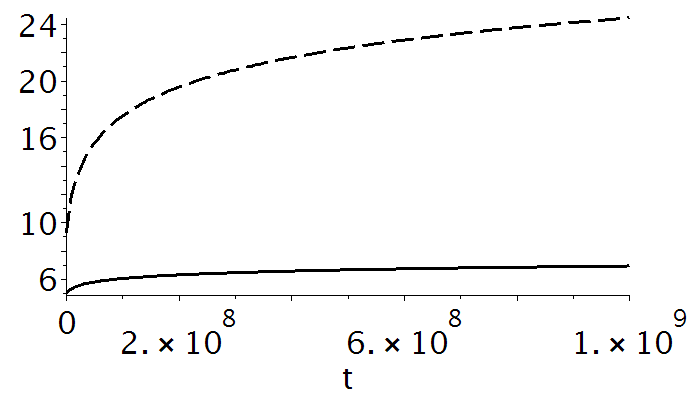
It was the Einstein frame. A transition to the Jordan frame, written explicitly using Eq. (18), gives no new results simply because of a very slow variation of the extra-space metric.
6 Conclusion
The space domains containing the expanding extra dimensions like those described above could exists in our Universe. It would be of interest to study light propagation from there. Also, ordinary matter could penetrate inside a domain possessing unusual properties, or they could be connected with our space through wormholes [41, 42, 27] It is also of interest to study the stability of such regions from the point of view of an external observer: do they expand or shrink?
Another possibility arises if we recall that the potential maximum separates two minima as in Fig. 1. In this case, a closed wall is formed [43], which could expand or shrink, sweeping out the internal domain. As was discussed in [34, 28, 29], shrinking walls could cause multiple formation of black holes in the Universe. It could solve the problem of primordial black hole formation [25, 30].
Acknowledgment
This work has been supported by the Ministry of Science and Higher Education of the Russian Federation, Project “Fundamental properties of elementary particles and cosmology” N 0723-2020-0041. The work of S.R/ was also supported by RFBR grant No. 19-02-00930, and the work of K.B. by RFBR grant No. 19-02-00346.
References
- [1] H. van Elst, J. E. Lidsey, and R. Tavakol. Quantum cosmology and higher-order Lagrangian theories. Classical Quant. Grav. 11, 2483–2497 (1994).
- [2] Raphael Bousso and Andrei D. Linde. Quantum creation of a universe with : Singular and nonsingular instantons. Phys. Rev. D 58, 083503 (1998).
- [3] J. J. Halliwell. Introductory Lectures on Quantum Cosmology (1990), arXiv: 0909.2566.
- [4] Nima Arkani-Hamed, Savas Dimopoulos, and G. R. Dvali. The Hierarchy problem and new dimensions at a millimeter. Phys. Lett. B 429, 263–272 (1998).
- [5] K. R. Dienes, E. Dudas, and T. Gherghetta. Grand unification at intermediate mass scales through extra dimensions. Nucl. Phys. B 537, 47–108 (1999).
- [6] Varun Sahni and Alexei A. Starobinsky. The Case for a positive cosmological Lambda term. Int. J. Mod. Phys. D 9, 373–444 (2000).
- [7] U. Günther, P. Moniz, and A. Zhuk. Nonlinear multidimensional cosmological models with form fields: Stabilization of extra dimensions and the cosmological constant problem. Phys. Rev. D 68 (4), 044010 (2003).
- [8] Sergey G. Rubin. Inhomogeneous extra space as a tool for the top-down approach. Adv. High Energy Phys., 2018, 2767410 (2018).
- [9] B. Greene and J. Levin. Dark energy and stabilization of extra dimensions. Journal of High Energy Physics 11, 96 (2007).
- [10] S. M. Carroll et al. Classical stabilization of homogeneous extra dimensions. Phys. Rev. D 66 (2), 024036 (2002).
- [11] S. Nasri, P. J. Silva, G. D. Starkman, and M. Trodden. Radion stabilization in compact hyperbolic extra dimensions. Phys. Rev. D 66 (4), 045029 (2002).
- [12] S. V. Ketov and H. Nakada. Inflation from (R + Rn-2 ) gravity in higher dimensions. Phys. Rev. D 95 (10), 103507 (2017).
- [13] H. Kihara, M. Nitta, M. Sasaki, C.-M. Yoo, and I. Zaballa. Dynamical compactification and inflation in Einstein-Yang-Mills theory with higher derivative coupling. Phys. Rev. D 80 (6), 066004 (2009).
- [14] P. Candelas and S. Weinberg. Calculation of gauge couplings and compact circumferences from self-consistent dimensional reduction. Nuclear Physics B 237, 397–441 (1984).
- [15] S. V. Bolokhov and K. A. Bronnikov. On cosmology in nonlinear multidimensional gravity with multiple factor spaces. Grav. Cosmol. 24, 154–160 (2018).
- [16] P. G. O. Freund and M. A. Rubin. Dynamics of dimensional reduction. Physics Letters B 97, 233–235 (1980).
- [17] M. Yoshimura. Effective action and cosmological evolution of scale factors in higher-dimensional curved spacetime. Phys. Rev. D 30, 344–356 (1984).
- [18] K. A. Bronnikov, V. N. Melnikov, S. G. Rubin, and I. V. Svadkovsky. Nonlinear multidimensional gravity and the Australian dipole. General Relativity and Gravitation 45, 2509–2528 (2013).
- [19] Alexei A. Starobinsky. A new type of isotropic cosmological models without singularity. Phys. Lett. B 91, 99–102 (1980).
- [20] B. Paul. Removing the Ostrogradski ghost from degenerate gravity theories. Phys. Rev. D 96 (4), 044035 (2017).
- [21] John F. Donoghue. General relativity as an effective field theory: The leading quantum corrections. Phys. Rev. D 50, 3874–3888 (1994).
- [22] C. P. Burgess. An Introduction to Effective Field Theory. Annual Review of Nuclear and Particle Science 57, 329–362 (2007).
- [23] Yana Lyakhova, Arkady A. Popov, and Sergey G. Rubin. Classical evolution of subspaces. Eur. Phys. J. C 78 (9), 764 (2018).
- [24] Júlio C. Fabris, Arkady A. Popov, and Sergey G. Rubin. Multidimensional gravity with higher derivatives and inflation. Phys. Lett. B 806 135458 (2020).
- [25] M. Yu. Khlopov and S. G. Rubin. Cosmological Pattern of Microphysics in the Inflationary Universe. Kluwer Academic Publishers, P.O. Box 17, 3300 AA Dordrecht, The Netherlands, 2004.
- [26] Maxim Yu. Khlopov, Sergei G. Rubin, and Alexander S. Sakharov. Possible origin of antimatter regions in the baryon dominated universe. Phys. Rev. D 62, 083505 (2000).
- [27] S. G. Rubin. Interpenetrating subspaces as a funnel to extra space. Physics Letters B 759, 622–625 (2016).
- [28] Konstantin M. Belotsky, Vyacheslav I. Dokuchaev, Yury N. Eroshenko, Ekaterina A. Esipova, Maxim Yu. Khlopov, Leonid A. Khromykh, Alexander A. Kirillov, Valeriy V. Nikulin, Sergey G. Rubin, and Igor V. Svadkovsky. Clusters of primordial black holes. Eur. Phys. J. C 79 (3), 246 (2019).
- [29] S. G. Rubin, M. Y. Khlopov, and A. S. Sakharov. Primordial black holes from non-equilibrium second order phase transition, arXiv: hep-ph/0005271.
- [30] Maxim Yu Khlopov. Primordial black holes. Research in Astronomy and Astrophysics 10 (6), 495–528 (2010).
- [31] S.V. Bolokhov and K.A. Bronnikov. On nonlinear multidimensional gravity and the Casimir effect. Grav. Cosmol. 22, 323–328 (2016).
- [32] S.V. Bolokhov and K.A. Bronnikov. Cosmology in nonlinear multidimensional gravity and the Casimir effect. J. Phys. Conf. series 798, 012091 (2017); arXiv: 1612.04177.
- [33] K.A. Bronnikov and S.G. Rubin, Self-stabilization of extra dimensions, Phys. Rev. D 73, 124019 (2006); gr-qc/0510107.
- [34] K.A. Bronnikov and S.G. Rubin, Black Holes, Cosmology and Extra Dimensions (World Scientific, 2013).
- [35] S.V. Ketov and A.A. Starobinsky, Inflation and nonminimal scalar-curvature coupling in gravity and supergravity, J. Cosmol. Astropart. Phys. 2012, 022 (2012), 022.
- [36] K. Bamba and S.D. Odintsov, Inflationary cosmology in modified gravity theories. Symmetry 7, 220 (2015).
- [37] S.V. Bolokhov, K.A. Bronnikov, and M.V. Skvortsova, The Schwarzschild singularity: a semiclassical bounce? Grav. Cosmol. 24, 315–320 (2018); arXiv: 1808.03717.
- [38] K.A. Bronnikov, S.V. Bolokhov, and M.V. Skvortsova Matter accretion versus semiclassical bounce in Schwarzschild interior, Universe 6, 178 (2020); arXiv: 2009.06330.
- [39] J. Mueller and L. Biskupek, Variations of the gravitational constant from lunar laser ranging data. Class. Quantum Gravity 24, 4533–4538 (2007).
- [40] E.V. Pitjeva, Updated IAA RAS planetary ephemerides-EPM2011 and their use in scientific research. Astron. Vestnik 47 (5), 419–435 (2013); arXiv: 1308.6416.
- [41] K.A. Bronnikov and M.V. Skvortsova. Wormholes leading to extra dimensions. Grav. Cosmol. 22, 316–322 (2016); arXiv: 1608.04974.
- [42] K.A. Bronnikov, P.A. Korolyov, A. Makhmudov, and M.V. Skvortsova. Wormholes and black universes communicated with extra dimensions. J. Phys. Conf. series 798, 012090 (2017); arXiv: 1612.04205.
- [43] M. Yu. Khlopov, R. V. Konoplich, S. G. Rubin, and A. S. Sakharov. Formation of black holes in first order phase transitions, arXiv: hep-ph/9807343.