跳到论文正文
W Papers独立论文阅读器 arXiv:2107.13610 论文正文 计算阅读时间 · 0%
引用这篇论文根据当前论文元数据生成,正式投稿前建议核对。


License: arXiv.org perpetual non-exclusive license
arXiv:2107.13610v2 [cs.LG] 11 Nov 2022

Large sample spectral analysis of graph-based multi-manifold clustering

Nicolás García Trillos garciatrillo@wisc.edu Affiliation: Department of Statistics Affiliation: University of Wisconsin Affiliation: Madison, Wisconsin, USA    Pengfei He hepengf1@msu.edu Affiliation: Department of Statistics and Probability Affiliation: Michigan State University Affiliation: East Lansing, MI, USA    Chenghui Li cli539@wisc.edu Affiliation: Department of Statistics Affiliation: University of Wisconsin Affiliation: Madison, Wisconsin, USA
Abstract

In this work we study statistical properties of graph-based algorithms for multi-manifold clustering (MMC). In MMC the goal is to retrieve the multi-manifold structure underlying a given Euclidean data set when this one is assumed to be obtained by sampling a distribution on a union of manifolds ℳ=ℳ1∪⋯∪ℳN\mathcal{M}=\mathcal{M}_{1}\cup\dots\cup\mathcal{M}_{N} that may intersect with each other and that may have different dimensions. We investigate sufficient conditions that similarity graphs on data sets must satisfy in order for their corresponding graph Laplacians to capture the right geometric information to solve the MMC problem. Precisely, we provide high probability error bounds for the spectral approximation of a tensorized Laplacian on ℳ\mathcal{M} with a suitable graph Laplacian built from the observations; the recovered tensorized Laplacian contains all geometric information of all the individual underlying manifolds. We provide an example of a family of similarity graphs, which we call annular proximity graphs with angle constraints, satisfying these sufficient conditions. We contrast our family of graphs with other constructions in the literature based on the alignment of tangent planes. Extensive numerical experiments expand the insights that our theory provides on the MMC problem.

††shortheadings: Spectral Analysis for Graph-based MMC / García Trillos, He and Li††firstpage: 1
keywords
multi-manifold clustering, graph Laplacian, spectral convergence, manifold learning, discrete to continuum limit.

1 Introduction

11footnotetext: All authors contributed equally to this work. Their names are listed in alphabetical order by last name.

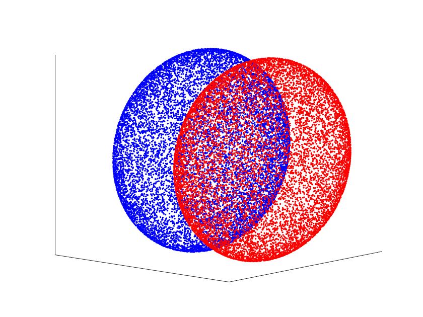
In this work we study the problem of multi-manifold clustering (MMC) from the perspective of spectral geometry. Multi-manifold clustering is the task of identifying the structure of multiple manifolds that underlie an observed data set X={x1,…,xn}X=\{x_{1},\dots,x_{n}\}, its main challenge being that in general the underlying manifolds may be non-linear, may intersect with each other, and may have different dimensions (see Figures 3-3 and Figures 40-40 for some illustrations). While spectral methods for learning have been analyzed by several authors throughout the past two decades in settings as varied as unsupervised, semi-supervised, and supervised learning, less is known about their theoretical guarantees for the specific multi-manifold clustering problem. We analyze MMC algorithms that are based on the construction of suitable similarity graph representations for the data and in turn on the spectra of their associated graph Laplacians. We provide statistical error guarantees for the identification of the underlying manifolds as well as for the recovery of their individual geometry.

Refer to caption
Figure 1:
Refer to caption
Figure 2:
Refer to caption
Figure 3:
Figure 3 illustrates two intersecting ellipsoids (two dimensional). A good multi-manifold clustering algorithm must identify the two underlying ellipsoids. Figure 3 and Figure 3 show the spectral clustering with kk-NN graph and annular proximity graph with angle constraint, respectively; see section 3.

As for most spectral approaches to clustering, we are interested in studying spectral properties of graph Laplacian operators of the form

Δn​u​(xi):=∑ωi​j​(u⁡(xi)−u⁡(xj)),xi∈X.\Delta_{n}u(x_{i}):=\sum\omega_{ij}(u(x_{i})-u(x_{j})),\quad x_{i}\in X. (1.1)

Here, the ωi​j\omega_{ij} are appropriately defined symmetric weights that in general depend on the proximity of points xi,xjx_{i},x_{j}, and, importantly, on a mechanism that detects when points belong to different manifolds even if lying close to each other. Once the graph Laplacian is constructed, we follow the spectral clustering algorithm: the first NN eigenvectors of Δn\Delta_{n} (denoted ψ1,…,ψN\psi_{1},\dots,\psi_{N}) are used to build an embedding of the data set XX into ℝN\mathbb{R}^{N}:

xi∈X⟼(ψ1​(xi)ψN​(xi))∈ℝN.x_{i}\in X\longmapsto\left(\begin{matrix}\psi_{1}(x_{i})\\ \vdots\\ \psi_{N}(x_{i})\end{matrix}\right)\in\mathbb{R}^{N}.

In turn, with the aid of a simple clustering algorithm such as kk-means the embedded data set is clustered. A successful algorithm will produce clusters that are in agreement with the different manifolds underlying the data set.

As can be imagined, the success of spectral clustering when applied to MMC problems relies strongly on the specific similarity weights ωi​j\omega_{ij} that determine the graph Laplacian, its eigenvectors, and ultimately the partitioning of the data. In the literature, authors have considered different types of mechanisms to discriminate points that lie on different manifolds. Some strategies include the use of local tangent planes from data Arias-Castro et al. 2017; Goh and Vidal 2007; Elhamifar and Vidal 2011; Wang et al. 2011 (whose angles are compared), and the construction of paths between different points (e.g. geodesics) that are considered admissible if they do not exhibit sudden turns (effectively imposing a curvature constraint) Babaeian et al. 2015. All these methods are inspired by heuristics that are meaningful at the continuum level (i.e. the infinite data setting) and use second order geometric information to detect the different intersecting manifolds. While these heuristics provide practical insights, in general they do not guarantee the success of the employed methodologies for MMC at the finite sample level. Part of the motivation for this work is precisely to establish a more concrete and mathematically precise link between the heuristic motivation at the continuum level and the actual methodologies that are used in practice. It is worth highlighting that widely known graph constructions such as ε\varepsilon-proximity graphs or kk-NN graphs used for standard data clustering tasks (typically aimed at detecting bottle-necks in data sets) are in general not suitable for MMC. To illustrate this, take for example Figure 3. There, we have used a kk-NN graph to build a graph Laplacian whose first non-trivial eigenvector has been used to obtain the partition illustrated in the figure; as can be observed, from the geometry induced by the kk-NN graph we are unable to distinguish the two underlying ellipsoids.

To start making the results presented in this paper more precise, let us suppose that the data set XX is obtained by sampling a distribution μ\mu supported on a set ℳ\mathcal{M} of the form

ℳ=ℳ1∪⋯∪ℳN,\mathcal{M}=\mathcal{M}_{1}\cup\dots\cup\mathcal{M}_{N}, (1.2)

where the ℳl\mathcal{M}_{l} are smooth compact connected manifolds with no boundary that for the moment are assumed to have the same dimension mm; the manifolds ℳl\mathcal{M}_{l} may have nonempty pairwise intersections, but these are assumed to have measure zero relative to the volume forms of each of the manifolds involved. The distribution μ\mu is assumed to be a mixture model taking the form

d​μ=w1​ρ1​d​volℳ1+⋯+wN​ρN​d​volℳN,d\mu=w_{1}\rho_{1}d\mathrm{vol}_{\mathcal{M}_{1}}+\dots+w_{N}\rho_{N}d\mathrm{vol}_{\mathcal{M}_{N}},

for smooth density functions ρl:ℳl→ℝ\rho_{l}:\mathcal{M}_{l}\rightarrow\mathbb{R} and positive weights wiw_{i} that add to one; henceforth we use d​volℳld\mathrm{vol}_{\mathcal{M}_{l}} to denote integration with respect to the Riemannian volume form associated to ℳl\mathcal{M}_{l}. A tensorized Laplacian Δℳ\Delta_{\mathcal{M}} acting on functions ff on ℳ\mathcal{M} (which will be written as f=(f1,…,fN)f=(f_{1},\dots,f_{N}), where fl:ℳl→ℝf_{l}:\mathcal{M}_{l}\rightarrow\mathbb{R}) can be defined according to

Δℳ​f:=(w1​Δℳ1​f1,…,wN​ΔℳN​fN),\Delta_{\mathcal{M}}f:=(w_{1}\Delta_{\mathcal{M}_{1}}f_{1},\dots,w_{N}\Delta_{\mathcal{M}_{N}}f_{N}), (1.3)

where Δℳl\Delta_{\mathcal{M}_{l}} is a Laplacian operator mapping regular enough functions fl:ℳl→ℝf_{l}:\mathcal{M}_{l}\rightarrow\mathbb{R} into functions Δℳ​fl:ℳl→ℝ\Delta_{\mathcal{M}}f_{l}:\mathcal{M}_{l}\rightarrow\mathbb{R} according to

Δℳl​fl=−1ρl​divℳl​(ρl2​∇ℳlfl).\Delta_{\mathcal{M}_{l}}f_{l}=-\frac{1}{\rho_{l}}\mathrm{div}_{\mathcal{M}_{l}}\left(\rho_{l}^{2}\nabla_{\mathcal{M}_{l}}f_{l}\right).

In other words, the operator Δℳ\Delta_{\mathcal{M}} acts in a coordinatewise fashion, effectively treating each manifold ℳi\mathcal{M}_{i} independently. It is then straightforward to show that eigenfunctions of Δℳ\Delta_{\mathcal{M}} are spanned by functions of the form

(0,…,fl,…,0)(0,\dots,f_{l},\dots,0)

for some ll, where flf_{l} is an eigenfunction of Δℳl\Delta_{\mathcal{M}_{l}}. This means that the spectrum of Δℳ\Delta_{\mathcal{M}} splits the geometries of the ℳl\mathcal{M}_{l}. In particular, the different ℳl\mathcal{M}_{l} can be detected by retrieving the eigenfunctions with zero eigenvalue.

Our first main results (Theorem 2.6 and Theorem 2.8) state that, provided that the weights ωi​j\omega_{ij} defining the graph Laplacian operator Δn\Delta_{n} in (1.1) satisfy two conditions referred to as full inner connectivity and sparse outer connectivity, the eigenvalues (appropriately scaled) and eigenvectors of Δn\Delta_{n} approximate the eigenvalues and eigenfunctions of the tensorized Laplacian Δℳ\Delta_{\mathcal{M}}; we obtain high probability quantitative bounds for the error of this approximation. The bottom line is that our results imply that the spectral methods studied here are guaranteed, at least for large enough nn, to recover the underlying multi-manifold structure of the data; see Figure 3 for an illustration. Our work extends the growing literature of works that study the connection between graph Laplacians on data sets and their continuum analogues. This literature, which we review in section 1.1.1, has mostly focused on the smooth setting where multiple intersecting manifolds are not allowed.

In our second main result (Theorem 2.10), we present some results for the case when the dimensions of the manifolds ℳi\mathcal{M}_{i} do not agree. In this more general setting, the spectrum of the graph Laplacian Δn\Delta_{n} does not recover the tensorized geometry captured by Δℳ\Delta_{\mathcal{M}} as introduced earlier, but rather, only the tensorized geometry of the manifolds with the largest dimension, effectively quotienting out the geometric information of manifolds with dimension strictly smaller than the maximum dimension.

After presenting our general results, we move on to discussing specific examples of graph constructions that satisfy the full inner connectivity and sparse outer connectivity conditions. In particular, we discuss a family of annular proximity graphs with angle constraints (see section 3) that we show satisfies the desired connectivity conditions. In the final section of the paper, we present some insights into the behavior of this graph construction and its ability to tackle the MMC problem in concrete numerical examples, as well as present a performance comparison with other existing spectral-based MMC approaches.

1.1 Related work

In this section we provide an overview of some related works that study spectral clustering and its connection with manifold learning, as well as other works that study the specific multi-manifold clustering problem.

1.1.1 Spectral clustering and manifold learning

In the past two decades, several authors have attempted to establish precise connections between operators such as graph Laplacians built from random data and analogous differential operators defined at the continuum level. To make this connection mathematically precise, one can assume that the data are sampled from some distribution supported on a certain geometric object ℳ\mathcal{M}. In the setting where ℳ\mathcal{M} is a smooth compact manifold embedded in ℝd\mathbb{R}^{d} that has no boundary, several authors have studied the connection between ε\varepsilon-graph-based Laplacians and weighted versions of Laplace Beltrami operators on ℳ\mathcal{M}. For pointwise consistency results we refer the reader to Singer 2006; Hein et al. 2005; Hein et al. 2007; Belkin and Niyogi 2005; Ting et al. 2010; Giné and Koltchinskii 2006). Regarding spectral convergence of graph Laplacians, a notion of convergence that is relevant for spectral clustering, the regime n→∞n\rightarrow\infty and ε\varepsilon constant is studied in von Luxburg et al. 2008 and also in Singer and Wu 2017. The latter analyzes connection Laplacians, which are operators acting on vector fields as opposed to functions. Works that have studied regimes where ε\varepsilon is allowed to decay to zero include Tao and Shi 2020; Burago et al. 2014; García Trillos et al. 2019; Lu 2022; Calder and García Trillos 2022; Dunson et al. 2021; Wormell and Reich 2021. The mathematical theory around graph Laplacians in the smooth manifold setting has developed considerably and even regularity estimates of graph Laplacian eigenvectors are now available (see Calder et al. 2022).

In the setting of a smooth compact manifold ℳ\mathcal{M} with boundary, graph Laplacians are seen to behave differently around the manifold’s boundary than in their interior. This has been observed in works like Vaughn et al. 2019; Wu and Wu 2018, which study this setting and obtain expansions for graph Laplacians that hold all the way up to the boundary. Earlier works such as García Trillos and Slepčev 2018 use variational methods to provide spectral asymptotic consistency results in this setting but don’t obtain convergence rates nor describe the behavior of graph Laplacians close to the boundary. The work Lu 2022 provides rates for spectral convergence in the setting of manifolds with boundary and also considers the case where ℳ\mathcal{M} is of the form (1.2). However, in contrast to what we do here, the aim in Lu 2022 is not to analyze graph constructions that guarantee the recovery of the multi-manifold structure of the data, focusing instead on analyzing intrinsic proximity graphs to the union of the intersecting manifolds. Our analysis shares aspects and ideas with this and some of the other works previously mentioned, but to fulfill our goals we must introduce new constructions and estimates not currently available. In addition, to the best of our knowledge, we are the first to present an analysis of the full spectrum of graph Laplacians when data points are supported on a union of intersecting manifolds that have different dimensions. Previous work Arias-Castro 2011 had analyzed the null space of a graph Laplacian when the generators (manifolds), although potentially of different dimensions, were assumed to be separated from each other.

From a methodological perspective, it is also worth highlighting several other works that have studied the use of metrics different from the Euclidean one to build proximity graphs for clustering and other unsupervised learning tasks. The idea in those papers is to use the modified metrics to improve the performance of spectral clustering when applied to data sets with some special geometric structure. Examples include: Ahmed et al. 2015; Rosenfeld and Pfaltz 1966; Normand et al. 2011; Fischer et al. 2001; Chang and Yeung 2008; Little et al. 2020; Little et al. 2022. In a sense, our approach in this paper is in line with the general perspective taken in the previously mentioned works, only that in our case we have a different geometric structure in mind, i.e., we consider multiple intersecting manifolds.

1.1.2 Multi-manifold clustering

In contrast to the graph constructions which are analyzed in most of the works mentioned in section 1.1.1 (i.e. standard ε\varepsilon-graphs and kk-NN graphs), graph constructions for multi-manifold clustering must incorporate a mechanism to discriminate between points that lie on different manifolds. One such mechanism relies on the approximation of approximate tangent planes around every point. Pairs of nearby points are then endowed high weights whenever their corresponding tangent planes are aligned, as proposed in Arias-Castro et al. 2017. The recovery of tangent planes from data is a problem that has been studied theoretically in papers such as Aamari and Levrard 2018 (see also references within). The methodology proposed in Singer and Wu 2017, which uses a connection Laplacian, can be considered as a MMC algorithm since it also uses tangent plane information to inform the affinity between points. The LLMC algorithm from Goh and Vidal 2007 is also based on locally fitting planes to points and their nearest neighbors. Sparse Manifold Clustering and Embedding(SMCE) in Elhamifar and Vidal 2011 implicitly attempts to recover tangent planes too; a sparse representation of points in a neighborhood is sought via a local l1l^{1} optimization problem. Another work that considers affinities based on local tangent planes is Wang et al. 2011. In section 3.2 we will discuss some properties of the tangent plane based graphs and their effect on spectral clustering for MMC. Wang et al. 2014 also consider estimating tangent planes to solve the MMC problem, but now in a generalized setting where the ambient space is a curved manifold and not ℝd\mathbb{R}^{d}.

At a high level, all multi-manifold clustering algorithms use curvature information to detect pairs of points that, while close to each other, lie on different manifolds. Measuring the difference of tangent planes is one way to capture curvature, but there are alternative ways. For example, works like Chen and Lerman 2009b; Chen and Lerman 2009a use the notion of polar curvature between collections of points to define an algorithm known as spectral curvature clustering (SCC). In Chen and Lerman 2009a the authors present some theoretical analysis of SCC in the setting where the data are sampled from multiple flats with the same dimension. In Arias-Castro et al. 2011, a localized spectral curvature clustering algorithm is proposed to find local curvature information by constructing similarity graphs that are obtained by aggregating certain alignment score for a collection of data tuples of high enough order. This method is computationally too intensive given that it requires to consider tuples of order larger than the dimension of the manifolds. Besides, from a theoretical perspective, the method scales very poorly with the dimensionality of the underlying manifolds, and the authors indicate that it can only solve the MMC problem in the setting of intersecting curves, i.e. 1d manifolds.

Curvature can also be captured by measuring how quickly paths turn as proposed in Babaeian et al. 2015. Our graph construction from section 3 is inspired by the one proposed in Babaeian et al. 2015, but with some important differences that we will motivate and explain throughout the paper. These differences, in particular, allow us to provide a comprehensive theoretical analysis and provide theoretical guarantees for the success of our algorithms.

To wrap up this brief literature review, it is worth mentioning a special setting where the manifolds ℳl\mathcal{M}_{l} are linear subspaces of the ambient space. In that case, the multi-manifold clustering problem reduces to subspace clustering (SubC), a problem that has received considerable attention in the past decades due to its multiple applications in tasks such as image segmentation, motion segmentation, and image representation (see Vidal 2011). Many algorithms in SubC rely strongly on the assumed global flat structure of the data and on the fact that the origin is known to lie on the intersection of the spaces. Unfortunately, these approaches can not be used directly for a general multi-manifold clustering task, so we will not discuss them in more detail. Conversely, while it is possible to use general MMC approaches to solve SubC problems, it is clear that the performance of general MMC methods will in general be far from satisfactory when compared to the performance of SubC approaches, which actively target the subspace structure of the manifolds. We refer the reader interested in the SubC problem to the following list of papers and their references: Boult and Brown 1991; Yan and Pollefeys 2006; Zhang et al. 2012; Park et al. 2014; Vidal et al. 2005; Ying Wu et al. 2001; Vidal et al. 2005; Ying Wu et al. 2001; Elhamifar and Vidal 2009; Elhamifar and Vidal 2010; Oswal and Nowak 2018; Liu et al. 2010.

1.2 Contributions and outline

We summarize our contributions as follows:

  • •

    We analyze graph Laplacians on families of proximity graphs when the nodes of the graphs are random data points that are supported on a union of unknown intersecting manifolds. The manifolds may all have different dimensions.

  • •

    We introduce two sufficient conditions that similarity graphs must satisfy in order to recover, from a graph Laplacian operator, the geometric information (as contained in the spectrum of weighted Laplace-Beltrami operators) of the individual smooth manifolds underlying the data set. These conditions are referred to as full inner connectivity and sparse outer connectivity.

  • •

    We introduce and analyze annular proximity graphs and their effect on multi-manifold clustering. These are simple extensions of ε\varepsilon-proximity graphs that nonetheless can be shown to be, theoretically and numerically, better than the vanilla ε\varepsilon-graphs for multi-manifold clustering.

  • •

    We analyze a family of annular proximity graphs with angle constraints. This family is shown to satisfy the full inner connectivity and sparse outer connectivity conditions when their parameters are tuned appropriately. We contrast this construction with other constructions such as those based on local PCA, which in general do not satisfy the full inner connectivity condition.

  • •

    Through numerical examples and some heuristic computations, we provide further insights into the use of spectral methods for multi-manifold clustering.

The rest of the paper is organized as follows. Our theoretical framework is presented in section 2, where we formalize the setting for the multi-manifold clustering problem, introduce the definitions of sparsely outer connected and fully inner connected similarity graphs, and state our main theoretical results. In our first results, the ones in section 2.3, we assume that all underlying manifolds have the same dimension, and in section 2.4 we extend to settings where the dimensions of the underlying manifolds can be different. In section 3 we discuss an example of a graph construction that satisfies the full inner connectivity and sparse outer connectivity conditions. In section 4 we present a series of numerical experiments whose goal is to illustrate the theory developed throughout the paper and highlight some drawbacks of the MMC methods discussed in the paper. In Appendix A we present the proofs of all the results from sections 2.3 and 2.4.

2 Set up and main results

Let {ℳl}l=1N\{\mathcal{M}_{l}\}_{l=1}^{N} be a collection of NN smooth, compact manifolds without boundary embedded in ℝd\mathbb{R}^{d}. We denote by mlm_{l} the dimension of manifold ℳl\mathcal{M}_{l} and m=maxl=1,…,N⁡{ml}m=\max_{l=1,\dots,N}\{m_{l}\}. Let ℳ\mathcal{M} be the union:

ℳ:=ℳ1∪⋯∪ℳN.\mathcal{M}:=\mathcal{M}_{1}\cup\dots\cup\mathcal{M}_{N}.

Let X={x1,…,xn}X=\{x_{1},\dots,x_{n}\} be i.i.d. samples from a distribution μ\mu on ℳ\mathcal{M} of the form:

d​μ=∑l=1Nwl​ρl​(x)​d​volℳl​(x),where​wl>0,∑l=1Nwl=1.d\mu=\sum_{l=1}^{N}w_{l}\rho_{l}(x)d\mathrm{vol}_{\mathcal{M}_{l}}(x),\ \ \text{where}\ w_{l}>0,\quad\sum_{l=1}^{N}w_{l}=1. (2.1)

In the above, for each ll, d​volℳld\mathrm{vol}_{\mathcal{M}_{l}} is used to denote integration with respect to the Riemannian volume form associated to the manifold ℳl\mathcal{M}_{l}, and the probability density ρl:ℳl→ℝ\rho_{l}:\mathcal{M}_{l}\rightarrow\mathbb{R} is assumed to be C2​(ℳl)C^{2}(\mathcal{M}_{l}) and satisfy

1cρ≤ρl(x)≤cρ,∀l=1,…,N\frac{1}{c_{\rho}}\leq\rho_{l}(x)\leq c_{\rho},\quad\forall l=1,\dots,N

for some positive constant cρ>1c_{\rho}>1. We use μl\mu_{l} to denote the probability measure ρl​d​volℳl\rho_{l}d\mathrm{vol}_{\mathcal{M}_{l}}. Notice that from (2.1) it follows that the number of data points nln_{l} in manifold ℳl\mathcal{M}_{l} is with very high probability within the interval [wl​n−t,wl​n+t][w_{l}n-t,w_{l}n+t] for some tolerance level tt at least in the order of n\sqrt{n}.

While we will not require the manifolds ℳl\mathcal{M}_{l} to be separated from each other in a distance sense (i.e., we allow manifolds to intersect with each other), we will assume that they are sufficiently “well separated” in an angular sense that we specify below and that we illustrate in Figure 4.

Assumption 1.

For every l,kl,k we assume:

  1. 1.

    The intersection ℳl​k:=ℳl∩ℳk\mathcal{M}_{lk}:=\mathcal{M}_{l}\cap\mathcal{M}_{k} is either the empty set or a smooth manifold of dimension mk​lm_{kl} satisfying 0≤mk​l<min⁡{ml,mk}0\leq m_{kl}<\min\{m_{l},m_{k}\}. In particular, ℳl​k\mathcal{M}_{lk} is of measure zero according to volℳl\mathrm{vol}_{\mathcal{M}_{l}} and volℳk\mathrm{vol}_{\mathcal{M}_{k}}.

  2. 2.

    For every point xx in ℳl∩ℳk\mathcal{M}_{l}\cap\mathcal{M}_{k} we have:

    supv∈𝒯xℳl​k⟂l,v~∈𝒯xℳl​k⟂k|∠(v,v~)−π2|≤β,\sup_{v\in\mathcal{T}_{x}\mathcal{M}_{lk}^{\perp_{l}},\widetilde{v}\in\mathcal{T}_{x}\mathcal{M}_{lk}^{\perp_{k}}}|\angle(v,\widetilde{v})-\frac{\pi}{2}|\leq\beta, (2.2)

    for some fixed β\beta strictly smaller than π2\frac{\pi}{2}. In the above, ∠⁡(v,v~)\angle(v,\widetilde{v}) denotes the angle between vectors v,v~v,\tilde{v} (recall that all manifolds are embedded in the ambient space ℝd\mathbb{R}^{d}), and 𝒯xℳl​k⟂l\mathcal{T}_{x}\mathcal{M}_{lk}^{\perp_{l}} denotes the orthogonal complement of 𝒯x​ℳl​k\mathcal{T}_{x}\mathcal{M}_{lk} in 𝒯x​ℳl\mathcal{T}_{x}\mathcal{M}_{l}, and 𝒯xℳl​k⟂k\mathcal{T}_{x}\mathcal{M}_{lk}^{\perp_{k}} is defined analogously.

Refer to caption

Figure 4: 𝒯​ℳk​l⟂k\mathcal{T}\mathcal{M}_{kl}^{\perp k} is the orthogonal complement of 𝒯​ℳk​l\mathcal{T}\mathcal{M}_{kl} in 𝒯​ℳk\mathcal{T}\mathcal{M}_{k}. 𝒯​ℳk​l⟂l\mathcal{T}\mathcal{M}_{kl}^{\perp l} is defined analogously. The second part in Assumption 1 is better satisfied when the angle between these spaces is close to ninety degrees.

In the above, and in the remainder, we use 𝒯x​ℳl\mathcal{T}_{x}{\mathcal{M}_{l}} to denote the tangent plane to ℳl\mathcal{M}_{l} at the point x∈ℳlx\in\mathcal{M}_{l}; also, we use 𝒯​ℳl\mathcal{T}\mathcal{M}_{l} to denote the tangent bundle associated to ℳl\mathcal{M}_{l}. Notice that the second condition in Assumption 1 states that if two manifolds ℳl\mathcal{M}_{l} and ℳk\mathcal{M}_{k} do intersect, they do so in a non-tangential way; see Figure 4 below.

2.1 Fully inner connected, and sparsely outer connected graphs

We endow the data set XX with a weighted graph structure (X,ω)(X,\omega), where the weights ω\omega are specified by the data. In this section we present the definitions of fully inner connected and sparsely outer connected graphs. The notion of full inner connectivity depends on a prespecified family of base proximity graphs that we introduce next.

Definition 2.1.

Given 0≤ε−<ε+0\leq\varepsilon_{-}<\varepsilon_{+} and data points xi,xjx_{i},x_{j}, we define their ε+,ε−\varepsilon_{+},\varepsilon_{-}-weight as:

ωi​jε+,ε−:={1 if ​ε−≤|xi−xj|≤ε+0otherwise.\omega_{ij}^{\varepsilon_{+},\varepsilon_{-}}:=\begin{cases}1\quad\text{ if }\varepsilon_{-}\leq|x_{i}-x_{j}|\leq\varepsilon_{+}\\ 0\quad\text{otherwise}.\end{cases}

We use ωi​jε\omega_{ij}^{\varepsilon} as shorthand notation for ωi​jε,0\omega_{ij}^{\varepsilon,0}. Notice that with this definition we have the identity:

ωy​xε+,ε−=ωy​xε+−ωy​xε−.\omega^{\varepsilon_{+},\varepsilon_{-}}_{yx}=\omega^{\varepsilon_{+}}_{yx}-\omega^{\varepsilon_{-}}_{yx}.
Remark 2.2.

The above definition extends the notion of ε\varepsilon-proximity graph and in principle allows pairs of points that are too close to each other to have zero weight. While in the literature this annular proximity graphs have not been given any attention, we will see later on that this extended notion is convenient from qualitative and quantitative points of view for the MMC problem; see the discussion surrounding Lemmas 3.19 and 3.20.

Definition 2.3 (Fully inner Connected graphs).

Let X=x1,…,xnX={x_{1},\dots,x_{n}} be samples from μ\mu as defined in (2.1). A weighted graph (X,ω)(X,\omega) is said to be fully inner connected relative to the ε+,ε−\varepsilon_{+},\varepsilon_{-} weights as n→∞n\rightarrow\infty, if with probability 1−C1​(n)1-C_{1}(n), where C1​(n)→0C_{1}(n)\rightarrow 0 as n→∞n\rightarrow\infty, for any pair of points xi,xjx_{i},x_{j} belonging to the same manifold ℳk\mathcal{M}_{k} we have ωxi,xj=ωxi,xjε+,ε−\omega_{x_{i},x_{j}}=\omega^{\varepsilon_{+},\varepsilon_{-}}_{x_{i},x_{j}}.

Remark 2.4.

It is possible to generalize the definition of full inner connectivity considered here and adapt it to other base proximity graph constructions like weighted proximity graphs. Indeed, the essential requirement that the full inner connectivity condition imposes on (X,ω)(X,\omega) is that it should behave like a graph that can capture the underlying geometry of each individual manifold. We have chosen annular proximity graphs here because 1) they can be used to capture the geometry of the underlying manifolds (as shown by our analysis: just take Theorems 2.6 and 2.8 and consider the case where the number of manifolds is equal to one), and 2) because they introduce an extra degree of flexibility that, as we show later on, allows us to prove better recovery guarantees for MMC than what we can show for standard ε\varepsilon-graphs; see Remark 2.2.

Next, we introduce the notion of spare outer connectivity.

Definition 2.5 (Sparsely Outer Connected graphs).

Let X=x1,…,xnX={x_{1},\dots,x_{n}} be samples from μ\mu as defined in (2.1), and let (X,ω)(X,\omega) be a weighted graph. Let Ns​lN_{sl} be the number of connections between xi∈ℳsx_{i}\in\mathcal{M}_{s} and xj∈ℳlx_{j}\in\mathcal{M}_{l} such that ωi​j>0\omega_{ij}>0, and let

N0:=maxl≠s⁡{Nl​s}.N_{0}:=\max_{l\not=s}\{N_{ls}\}.

The graph is said to be sparsely outer connected relative to ε+\varepsilon_{+} and ε−\varepsilon_{-} converging to zero as n→∞n\rightarrow\infty if with probability one N0n2​(ε+m+2−ε−m+2)→0\frac{N_{0}}{n^{2}(\varepsilon_{+}^{m+2}-\varepsilon_{-}^{m+2})}\rightarrow 0 as n→∞n\rightarrow\infty. We recall that m=maxl=1,…,N⁡mlm=\max_{l=1,\dots,N}m_{l}.

The above notions will capture the intuitive desire of giving high weights to pairs of points that are close to each other when they belong to the same manifold (full inner connectivity condition) and to give low weights to pairs of points when they lie on different manifolds (sparse outer connectivity condition). These notions are geometric adaptations to the setting of interest of general notions explored in the literature to describe the feasibility of a clustering problem. We elaborate on this next.

In the setting considered in Ng et al. 2001, for example, given a network (X,W)(X,W), four conditions on the network (that depend on the Laplacian and degree function of the network) are proposed to ensure that a certain spectral embedding constructed from (X,W)(X,W) maps the original set of nodes XX to points that are close to a set of orthogonal vectors in Euclidean space; notice that the conditions in Ng et al. 2001 do not rely on any specific modelling assumption on the generative process that produces the data set XX. Works like Schiebinger et al. 2015 and García Trillos et al. 2021 have taken a different perspective and introduced sufficient geometric conditions on certain families of generative models that, at the “ground-truth” level, guarantee the feasibility of a certain ground-truth level clustering problem. These works then show that, when their proposed modelling assumptions hold, the conditions in Ng et al. 2001 are satisfied with high probability by certain network constructions (X,W)(X,W), where XX is a set of samples from the generative model, and WW is a suitable weight matrix over XX. The notions of inner connectivity and outer connectivity considered here can be interpreted as conditions that a given weight matrix WW built over a data set XX sampled from a model like (2.1) must satisfy in order for the network (X,W)(X,W) to: 1) satisfy the conditions in Ng et al. 2001 and 2) have clusters that are consistent with the underlying manifolds in the generative model (2.1). In this sense, the results that we present in this paper are analogous to those in Schiebinger et al. 2015; García Trillos et al. 2021, except that the geometric structure of the generative models in our paper is substantially different from the ones in those works. Other works in the literature such as Vu 2018 have considered other types of “clusterability” conditions, requiring data points within each cluster to be close to each other and points from different clusters to be far away from each other. These conditions are certainly not satisfied in this paper, mainly because the separation between manifolds can in fact be equal to zero.

Before we finish this section, we remark that the discussion in the upcoming sections 2.2-2.4 will not be restricted to any particular graph construction. In the results presented there, we quantify the error of approximation of the spectra of tensorized Laplacians at the continuum level from the graph Laplacian associated to (X,ω)(X,\omega). This approximation error will naturally depend on the quantities C1​(n)C_{1}(n) and N0N_{0} appearing in the definition of the inner and outer connectivity conditions. In section 3, we provide one example of a family of graphs that satisfies the inner and outer connectivity conditions. The graphs in that family are obtained by pruning an ε+,ε−\varepsilon_{+},\varepsilon_{-} graph, removing edges between points for which there is no almost straight path connecting them. In section 3.2, we discuss other popular choices of weights ω\omega that are based on the comparison of local tangent planes, but that, as we will discuss, do not, in general, satisfy the full inner connectivity condition.

2.2 Basic properties of the spectrum of the operator Δℳ\Delta_{\mathcal{M}}

In order to state our main theoretical results in sections 2.3 and 2.4 we first discuss some basic properties of the spectrum of the operator Δℳ\Delta_{\mathcal{M}} in (1.3) and its relation to the MMC problem.

Let L2​(μ)L^{2}(\mu) be the space of NN tuples (f1,…,fN)(f_{1},\dots,f_{N}) where each fl∈L2​(μl)f_{l}\in L^{2}(\mu_{l}). We endow the space L2​(μ)L^{2}(\mu) with the tensorized inner product:

⟨f,g⟩L2​(μ):=∑l=1Nwl​⟨fl,gl⟩L2​(μl)=∑l=1Nwl​∫ℳlfl​(x)​gl​(x)​d​μl​(x),\langle f,g\rangle_{L^{2}(\mu)}:=\sum_{l=1}^{N}w_{l}\langle f_{l},g_{l}\rangle_{L^{2}(\mu_{l})}=\sum_{l=1}^{N}w_{l}\int_{\mathcal{M}_{l}}f_{l}(x)g_{l}(x)d\mu_{l}(x),

where f=(f1,…,fN)∈L2​(μ)f=(f_{1},\dots,f_{N})\in L^{2}(\mu) and g=(g1,…,gN)∈L2​(μ)g=(g_{1},\dots,g_{N})\in L^{2}(\mu). A tensorized Sobolev space H1​(μ)H^{1}(\mu) is defined as the space of f=(f1,…,fN)∈L2​(μ)f=(f_{1},\dots,f_{N})\in L^{2}(\mu) for which fl∈H1​(ℳl)f_{l}\in H^{1}(\mathcal{M}_{l}) for each l=1,…,Nl=1,\dots,N. In particular, for elements f∈H1​(μ)f\in H^{1}(\mu) the quantity

∑l=1Nwl2​∫ℳl|∇fl​(x)|2​ρl2​(x)​𝑑x\sum_{l=1}^{N}w_{l}^{2}\int_{\mathcal{M}_{l}}|\nabla f_{l}(x)|^{2}\rho^{2}_{l}(x)dx

is finite. We then define the weighted Dirichlet energy:

D⁡(f):={∑l=1Nwl2​∫ℳl|∇fl​(x)|2​ρl2​(x)​d​volℳl​(x), if ​f∈H1​(μ),+∞, if ​f∈L2​(μ)∖H1​(μ).D(f):=\begin{cases}\sum_{l=1}^{N}w_{l}^{2}\int_{\mathcal{M}_{l}}|\nabla f_{l}(x)|^{2}\rho^{2}_{l}(x)d\mathrm{vol}_{\mathcal{M}_{l}}(x),\quad\text{ if }f\in H^{1}(\mu),\\ +\infty,\quad\text{ if }f\in L^{2}(\mu)\setminus H^{1}(\mu).\end{cases} (2.3)

Now, notice that the operator Δℳ\Delta_{\mathcal{M}} is self-adjoint with respect to the inner product ⟨⋅,⋅⟩L2​(μ)\langle\cdot,\cdot\rangle_{L^{2}(\mu)} simply because each of the operators Δℳl\Delta_{\mathcal{M}_{l}} is self-adjoint w.r.t. ⟨⋅,⋅⟩L2​(μl)\langle\cdot,\cdot\rangle_{L^{2}(\mu_{l})} (e.g. see García Trillos and Slepčev 2018). Given that each L2​(ℳl,ρl)L^{2}(\mathcal{M}_{l},\rho_{l}) admits an orthonormal basis {flk}k∈ℕ\{f_{l}^{k}\}_{k\in\mathbb{N}} of eigenvectors of Δℳl\Delta_{\mathcal{M}_{l}}, we can see that the set of fk∈L2​(μ)f^{k}\in L^{2}(\mu) of the form

fk=(0,…,1wl​flk,…,0)f^{k}=(0,\dots,\frac{1}{\sqrt{w_{l}}}f_{l}^{k},\dots,0) (2.4)

for k∈ℕk\in\mathbb{N} and l=1,…,Nl=1,\dots,N is an orthonormal basis for L2​(μ)L^{2}(\mu). In addition, for such fkf^{k} we have

Δℳ​fk=(0,…,wlwl​Δℳl​flk,…,0)=wl​λ​(0,…,1wl​flk,…,0)=wl​λ​fk\Delta_{\mathcal{M}}f^{k}=(0,\dots,\frac{w_{l}}{\sqrt{w_{l}}}\Delta_{\mathcal{M}_{l}}f_{l}^{k},\dots,0)=w_{l}\lambda(0,\dots,\frac{1}{\sqrt{w_{l}}}f_{l}^{k},\dots,0)=w_{l}\lambda f^{k}

for some eigenvalue λ\lambda of Δℳl\Delta_{\mathcal{M}_{l}}. In conclusion, we can build an orthonormal basis for L2​(μ)L^{2}(\mu) consisting of eigenfunctions of Δℳ\Delta_{\mathcal{M}} of the form (2.4). From the above we can also conclude that the set of eigenvalues of Δℳ\Delta_{\mathcal{M}} is the set of numbers of the form wl​λw_{l}\lambda for some ll, where λ\lambda is an eigenvalue of Δℳl\Delta_{\mathcal{M}_{l}}. In terms of the Dirichlet energy defined in (2.3), the eigenvalues of Δℳ\Delta_{\mathcal{M}}, arranged in increasing order according to multiplicity, can be written as

λl=minS∈𝔖l⁡maxf∈S\{0}​D⁡(f)‖f‖L2​(μ)2.\lambda_{l}=\min_{S\in\mathfrak{S}_{l}}\max_{f\in S\backslash\{0\}}\frac{D(f)}{\|f\|_{L^{2}(\mu)}^{2}}. (2.5)

where 𝔖l\mathfrak{S}_{l} denotes the set of all linear subspaces of L2​(μ)L^{2}(\mu) of dimension ll.

Regarding the zero eigenvalue of Δℳ\Delta_{\mathcal{M}}, notice that since the manifolds ℳl\mathcal{M}_{l} were assumed to be connected, the multiplicity of the zero eigenvalue for the operator Δℳ\Delta_{\mathcal{M}} is equal to NN. Moreover, an orthonormal basis for this eigenspace is the set of functions of the form (0,…,cl​𝟙ℳl,…,0)(0,\dots,c_{l}\mathds{1}_{\mathcal{M}_{l}},\dots,0) where clc_{l} is a normalization constant. This observation is the key property that allows us to think of the multi-manifold clustering problem in terms of the spectrum of the operator Δℳ\Delta_{\mathcal{M}}. However, it should be clear that the tensorized Laplacian has much more information than that needed to solve the MMC problem.

For convenience, we also introduce Dirichlet energies associated to each manifold ℳl\mathcal{M}_{l}:

Dl​(fl):={∫ℳl|∇fl​(x)|2​ρl2​(x)​d​volℳl​(x), if ​fl∈H1​(μl),+∞if​f∈L2​(μl)∖H1​(μl).D_{l}(f_{l}):=\begin{cases}\int_{\mathcal{M}_{l}}|\nabla f_{l}(x)|^{2}\rho^{2}_{l}(x)d\mathrm{vol}_{\mathcal{M}_{l}}(x),\quad\text{ if }f_{l}\in H^{1}(\mu_{l}),\\ \\ +\infty\quad\text{if}f\in L^{2}(\mu_{l})\setminus H^{1}(\mu_{l}).\end{cases} (2.6)

2.3 Convergence results in the m1=⋯=mNm_{1}=\dots=m_{N} case

In this section we establish high probability error bounds between the spectrum of a rescaled version of the graph Laplacian Δn\Delta_{n} defined in (1.1) and the spectrum of Δℳ\Delta_{\mathcal{M}} under the additional assumption that all manifolds ℳk\mathcal{M}_{k} have the same dimension. The results presented in this section apply to generic weighted graphs (X,ω)(X,\omega), but the error estimates are only meaningful when the quantities N0N_{0}, C1​(n)C_{1}(n) and ε+\varepsilon_{+} from section 2.1 scale appropriately with the number of data points. In section 3 we present a specific construction for (X,ω)(X,\omega) where we can make our error estimates concrete.

In what follows we make the following assumptions on the parameters ε+,ε−,δ~,θ\varepsilon_{+},\varepsilon_{-},\widetilde{\delta},\theta. Here δ~\tilde{\delta} and θ\theta are small parameters that we use to tune the probabilities of some random events defined in corollary A.25.

Assumption 2.

We assume that the quantities ε+,ε−,δ~,θ\varepsilon_{+},\varepsilon_{-},\tilde{\delta},\theta satisfy:

  1. (1)

    ε+≤min{1,R2,CK−1/2,i0}\varepsilon_{+}\leq\min\{1,\frac{R}{2},CK^{-1/2},i_{0}\}, where R,KR,K are uniform upper bounds on the reach and on the absolute values of the sectional curvatures for all the manifolds, i0i_{0} is a lower bound on the injectivity radius of all manifolds, and CC is a constant no larger than 1.

  2. (2)

    ε−≤14​ε+\varepsilon_{-}\leq\frac{1}{4}\varepsilon_{+}; the 14\frac{1}{4} here is an arbitrary number smaller than 11.

  3. (3)

    cn1/m<δ~\frac{c}{n^{1/m}}<\widetilde{\delta}

  4. (4)

    C⁡(δ~+θ)≤12​cρC(\widetilde{\delta}+\theta)\leq\frac{1}{2c_{\rho}}, where 1cρ\frac{1}{c_{\rho}} is the lower bound of ρ\rho .

With the above assumptions we can make sure that with the underlying ε+,ε−\varepsilon_{+},\varepsilon_{-}-weighted graph we can approximate the operators Δℳk\Delta_{\mathcal{M}_{k}} in each of the ℳk\mathcal{M}_{k}; this part does not rely on the assumption that all manifolds have the same dimension, and only depends on the full inner connectivity property. For the spectrum of the graph Laplacian associated to (X,ω)(X,\omega) to successfully recover the spectrum of Δℳ\Delta_{\mathcal{M}} we need (X,ω)(X,\omega) to be fully inner connected and sparsely outer connected as we will make explicit in our first theorem.

Theorem 2.6 (Convergence rate for eigenvalues).

Let μ\mu be a probability measure on ℳ\mathcal{M} as in (2.1). Suppose that the ℳk\mathcal{M}_{k} forming the ℳ\mathcal{M} satisfy Assumptions 1, and assume also that m1=⋯=mNm_{1}=\dots=m_{N}. Let X={x1,…,xn}X=\{x_{1},\dots,x_{n}\} be i.i.d. samples from μ\mu. Let (X,ω)(X,\omega) be a symmetric weighted graph and let ℒ\mathcal{L} be the rescaled graph Laplacian:

ℒ​u​(x):=1n2​(ε+m+2−ε−m+2)​∑y∈Xωx​y​(u⁡(x)−u⁡(y)),x∈X,u:X→ℝ.\mathcal{L}u(x):=\frac{1}{n^{2}(\varepsilon_{+}^{m+2}-\varepsilon_{-}^{m+2})}\sum_{y\in X}\omega_{xy}(u(x)-u(y)),\quad x\in X,u:X\rightarrow\mathbb{R}. (2.7)

Suppose that the quantities δ~,θ,ε+,ε−\widetilde{\delta},\theta,\varepsilon_{+},\varepsilon_{-} satisfy Assumptions 2. Let λkε+,ε−\lambda_{k}^{\varepsilon_{+},\varepsilon_{-}} be the kk-th eigenvalue of ℒ\mathcal{L} and let λk\lambda_{k} be the kk-th eigenvalue of Δℳ\Delta_{\mathcal{M}}, where Δℳ\Delta_{\mathcal{M}} is the tensorized Laplacian from (1.3). Finally, let t:=n​ωmin2t:=\frac{n\omega_{\min}}{2}. Then there exists a constant CC (independent of kk) such that, with probability at least 1−∑l=1N(n​wl+t)​exp⁡(−C⁡(n​wl−t)​θ2​δ~m)−2​N​exp⁡(−2​t2n)−C1​(n)1-\sum_{l=1}^{N}(nw_{l}+t)\exp\left(-{C}(nw_{l}-t)\theta^{2}\widetilde{\delta}^{m}\right)-2N\exp\left(\frac{-2t^{2}}{n}\right)-C_{1}(n), for every k∈ℕk\in\mathbb{N} for which

C​δ~​λk+C⁡(θ+δ~)<1k,C\widetilde{\delta}\sqrt{\lambda_{k}}+C(\theta+\widetilde{\delta})<\frac{1}{k},

we have:

|λkε+,ε−−ση​λk|≤ek+C⁡(ε+​(λk+1)+θ+δ~ε+)​λk.\left|\lambda_{k}^{\varepsilon_{+},\varepsilon_{-}}-\sigma_{\eta}\lambda_{k}\right|\leq e_{k}+C\left(\varepsilon_{+}(\sqrt{\lambda_{k}}+1)+\theta+\frac{\widetilde{\delta}}{\varepsilon_{+}}\right)\lambda_{k}.

In the above, ek=C​N0n2​(ε+m+2−ε−m+2)​(1+C′​(λkm/2+1+δ~​λk+θ+δ~))e_{k}=\frac{CN_{0}}{n^{2}(\varepsilon_{+}^{m+2}-\varepsilon_{-}^{m+2})}\left(1+C^{\prime}(\lambda_{k}^{m/2+1}+\widetilde{\delta}\sqrt{\lambda_{k}}+\theta+\widetilde{\delta})\right), and C1​(n)C_{1}(n) and N0N_{0} are introduced in Definition 2.3 and Definition 2.5, respectively. The constant ση\sigma_{\eta} is given by:

ση:=∫ℝm|y1|2​η​(|y|)​𝑑y,\sigma_{\eta}:=\int_{\mathbb{R}^{m}}|y_{1}|^{2}\eta(|y|)dy, (2.8)

where η=𝟙r≤1\eta=\mathds{1}_{r\leq 1} and y1y_{1} is the first coordinate of yy.

Remark 2.7.
  1. 1.

    In general, we should expect a trade-off between the quantities C1​(n)C_{1}(n) and N0N_{0}. That is, in general, an attempt at making N0N_{0} smaller (i.e., erase connections between different manifolds) will typically result in a smaller probability of having a graph that is well connected within each manifold ℳl\mathcal{M}_{l}.

  2. 2.

    The benefits that come from taking ε−>0\varepsilon_{-}>0 for the MMC problem are not explicit in the error bounds from Theorem 2.6. However, as we will see later on, by tuning ε−\varepsilon_{-} appropriately, one can substantially eliminate connections between data points in different manifolds when one considers ε−∼ε+\varepsilon_{-}\sim\varepsilon_{+}. This means a substantial decrease in N0N_{0}. We explain this in Remark 3.17 for the specific annular graph construction with angle constraints. The fact that we can improve the performance of MMC algorithms by introducing ε+,ε−\varepsilon_{+},\varepsilon_{-}-graphs motivates the theoretical analysis that we present in the Appendix.

  3. 3.

    The proof of the estimates in Theorem 2.6 relies on a variational approach that compares Dirichlet energies at discrete and continuum levels. This approach has been used before in Burago et al. 2014; García Trillos et al. 2019; Lu 2022. However, the structure of the ε+,ε−\varepsilon_{+},\varepsilon_{-}-graph that we consider here forces us to modify the analysis and present new proofs. Even for a single manifold ℳ=ℳ1\mathcal{M}=\mathcal{M}_{1}, the analysis of graph Laplacians on ε+,ε−\varepsilon_{+},\varepsilon_{-}-graphs is a technical contribution of this work. The actual proof of Theorem 2.6 appears in section A.5 in the Appendix. Several technical preliminary results are established in the preceding sections.

  4. 4.

    The scaling factor relating ℒ\mathcal{L} and Δn\Delta_{n} in (2.7) is irrelevant in practice because the eigenvectors of Δn\Delta_{n} are the same as those for ℒ\mathcal{L}, and the ratio between eigenvalues of Δn\Delta_{n} coincides with the ratio of eigenvalues of ℒ\mathcal{L}. In other words, in practice we can work directly with Δn\Delta_{n} without having to compute the rescaling factor.

  5. 5.

    If we choose 1≫ε+≫(log⁡(n)n)1/m1\gg\varepsilon_{+}\gg\left(\frac{\log(n)}{n}\right)^{1/m}, then, with high probability, the error of approximation of eigenvalues scales like:

    N0n2​ε+m+2+(log⁡(n)n)1/mε++ε+.\frac{N_{0}}{n^{2}\varepsilon_{+}^{m+2}}+\frac{\left(\frac{\log(n)}{n}\right)^{1/m}}{\varepsilon_{+}}+\varepsilon_{+}.

    This result is analogous to results in Burago et al. 2014 and García Trillos et al. 2019, except that now we have the extra N0n2​ε+m+2\frac{N_{0}}{n^{2}\varepsilon_{+}^{m+2}} term. In order for this error estimate to converge to zero in the large data limit we thus need to require the graph to satisfy the sparse outer connectivity condition.

Theorem 2.8 (Convergence rate for eigenvectors).

Under the same setting and assumptions as in Theorem 2.6, for every k∈ℕk\in\mathbb{N} there is a constant ck=ck​(ℳ)c_{k}=c_{k}(\mathcal{M}) such that if

ek+C⁡(ε+​λk+ε+2+θ+δ~ε+)≤ck,e_{k}+C\left(\varepsilon_{+}\sqrt{\lambda_{k}}+\varepsilon_{+}^{2}+\theta+\frac{\widetilde{\delta}}{\varepsilon_{+}}\right)\leq c_{k},

then, with probability at least 1−∑l=1N(n​wl+t)​exp⁡(−C⁡(n​wl−t)​θ2​δ~m)−2​N​exp⁡(−2​t2n)−C1​(n)1-\sum_{l=1}^{N}(nw_{l}+t)\exp\left(-{C}(nw_{l}-t)\theta^{2}\widetilde{\delta}^{m}\right)-2N\exp\left(\frac{-2t^{2}}{n}\right)-C_{1}(n), for every vkv_{k} normalized eigenvector of ℒ\mathcal{L} with eigenvalue λk\lambda_{k}, there is a normalized eigenfunction fkf_{k} of Δℳ\Delta_{\mathcal{M}} with eigenvalue λk\lambda_{k} such that

∥fk−vk∥L2​(μn)≤[Cek+C(ε+λk+ε+2+θ+δ~ε+)]1/2+Cℳ,λδ~,\lVert f_{k}-v_{k}\lVert_{L^{2}(\mu^{n})}\leq\left[Ce_{k}+C\left(\varepsilon_{+}\sqrt{\lambda_{k}}+\varepsilon_{+}^{2}+\theta+\frac{\widetilde{\delta}}{\varepsilon_{+}}\right)\right]^{1/2}+C_{\mathcal{M},\lambda}\widetilde{\delta},

where eke_{k} is the same as in Theorem 2.6.

The proof of this theorem is presented in section A.6 in the Appendix.

Remark 2.9.

The sparse outer connectivity condition N0n2​(ε+m+2−ε−m+2)→0\frac{N_{0}}{n^{2}(\varepsilon_{+}^{m+2}-\varepsilon_{-}^{m+2})}\to 0 is imposed to guarantee the recovery of the full spectrum of the tensorized Laplacian in the large data limit. However, we highlight that our error estimates continue to be meaningful even if we only impose N0n2​(ε+m+2−ε−m+2)\frac{N_{0}}{n^{2}(\varepsilon_{+}^{m+2}-\varepsilon_{-}^{m+2})} to be asymptotically smaller than some small tolerance level cc.

2.4 Mixed dimensions.

We generalize our results from section 2.3 to a setting where the manifolds ℳk\mathcal{M}_{k} may have different dimensions. For convenience, we introduce some notation first.

Without the loss of generality we can assume that the manifolds ℳk\mathcal{M}_{k} are indexed in decreasing order of dimension, i.e. m=m1≥m2≥⋯≥mNm=m_{1}\geq m_{2}\geq\dots\geq m_{N}. We let NmaxN_{\max} be the number of manifolds with the maximum dimension mm, i.e. m1=⋯=mNmax>mNmax+1m_{1}=\dots=m_{N_{\max}}>m_{N_{\max}+1}. We set ℳmax:=ℳ1∪⋯∪ℳNmax\mathcal{M}_{\max}:=\mathcal{M}_{1}\cup\dots\cup\mathcal{M}_{N_{\max}} and write ⟨f,g⟩L2​(ℳmax)\langle f,g\rangle_{L^{2}(\mathcal{M}_{\max})} to represent:

⟨f,g⟩L2​(ℳmax)=∑i=1Nmaxwi​⟨fi,gi⟩L2​(μi)=∑i=1Nmaxwi​∫ℳifi​(x)​gi​(x)​d​μi​(x).\langle f,g\rangle_{L^{2}(\mathcal{M}_{\max})}=\sum_{i=1}^{N_{\max}}w_{i}\langle f_{i},g_{i}\rangle_{L^{2}(\mu_{i})}=\sum_{i=1}^{N_{\max}}w_{i}\int_{\mathcal{M}_{i}}f_{i}(x)g_{i}(x)d\mu_{i}(x).

We also use ∥f∥L2​(ℳmax)2=⟨f,f⟩L2​(ℳmax)\lVert f\rVert_{L^{2}(\mathcal{M}_{\max})}^{2}=\langle f,f\rangle_{L^{2}(\mathcal{M}_{\max})}.

Notice that with the above inner product we can identify (isometrically) elements in L2​(ℳmax)L^{2}(\mathcal{M}_{\max}) with elements in L2​(μ)L^{2}(\mu) that are zero outside of ℳmax\mathcal{M}_{\max}; throughout section A.7 in the Appendix we may use this identification without any further explanation. Finally, we use Δℳmax\Delta_{\mathcal{M}_{\max}} to denote the tensorized Laplacian (1.3) for ℳmax\mathcal{M}_{\max} (i.e. just as in (1.3) but with only the first NmaxN_{\max} coordinates); we use DmaxD_{\max} to denote the corresponding Dirichlet energy defined for L2​(ℳmax)L^{2}(\mathcal{M}_{\max}) functions.

Theorem 2.10.

Let μ\mu be a probability measure on ℳ\mathcal{M} as in (2.1). Suppose that the ℳk\mathcal{M}_{k} forming ℳ\mathcal{M} satisfy Assumptions 1, and let Nmax,ℳmax,ΔℳmaxN_{\max},\mathcal{M}_{\max},\Delta_{\mathcal{M}_{\max}} be defined as before. Set λ1,…,λN=0\lambda_{1},\dots,\lambda_{N}=0 and let λN+1≤λN+2≤…\lambda_{N+1}\leq\lambda_{N+2}\leq\dots be the list of non-zero eigenvalues of Δℳmax\Delta_{\mathcal{M}_{\max}} repeated according to multiplicity.

Let X={x1,…,xn}X=\{x_{1},\dots,x_{n}\} be i.i.d. samples from μ\mu, let (X,ω)(X,\omega) be a symmetric weighted graph, and let ℒ\mathcal{L} be the rescaled graph Laplacian from (2.7). Finally, suppose that the quantities δ~,θ,ε+,ε−\widetilde{\delta},\theta,\varepsilon_{+},\varepsilon_{-} satisfy Assumptions 2.

Then, for some constant C=C⁡(ℳ,μ)C=C(\mathcal{M},\mu), with probability at least

1−∑l=1N(n​wl+t)​exp⁡(−C⁡(n​wl−t)​θ2​δ~m)−2​N​exp⁡(−2​t2n)−C1​(n),1-\sum_{l=1}^{N}(nw_{l}+t)\exp\left(-\mathrm{C}(nw_{l}-t)\theta^{2}\widetilde{\delta}^{m}\right)-2N\exp\left(\frac{-2t^{2}}{n}\right)-C_{1}(n),

for every k∈ℕk\in\mathbb{N} for which

C​δ~​λk+C⁡(θ+δ~)<1k,C\widetilde{\delta}\sqrt{\lambda_{k}}+C(\theta+\widetilde{\delta})<\frac{1}{k},

we have:

|λkε+,ε−−ση​λk|≤ek+C⁡(ε+​(λk+1)+θ+δ~ε+)​λk.\left|\lambda_{k}^{\varepsilon_{+},\varepsilon_{-}}-\sigma_{\eta}\lambda_{k}\right|\leq e_{k}+C\left(\varepsilon_{+}(\sqrt{\lambda_{k}}+1)+\theta+\frac{\widetilde{\delta}}{\varepsilon_{+}}\right)\lambda_{k}.

In the above, ek=C​N0n2​(ε+m+2−ε−m+2)​(1+C′​(λkm/2+1+δ~​λk+θ+δ~))e_{k}=\frac{CN_{0}}{n^{2}(\varepsilon_{+}^{m+2}-\varepsilon_{-}^{m+2})}\left(1+C^{\prime}(\lambda_{k}^{m/2+1}+\widetilde{\delta}\sqrt{\lambda_{k}}+\theta+\widetilde{\delta})\right), and C1​(n)C_{1}(n) and N0N_{0} are introduced in Definition 2.3 and Definition 2.5, respectively.

In addition, there is a constant ck=ck​(ℳ)c_{k}=c_{k}(\mathcal{M}) such that if

ek+C⁡(ε+​λk+ε+2+θ+δ~ε+)≤ck,e_{k}+C\left(\varepsilon_{+}\sqrt{\lambda_{k}}+\varepsilon_{+}^{2}+\theta+\frac{\widetilde{\delta}}{\varepsilon_{+}}\right)\leq c_{k},

then, with probability at least 1−∑l=1N(n​wl+t)​exp⁡(−C⁡(n​wl−t)​θ2​δ~m)−2​N​exp⁡(−2​t2n)−C1​(n)1-\sum_{l=1}^{N}(nw_{l}+t)\exp\left(-{C}(nw_{l}-t)\theta^{2}\widetilde{\delta}^{m}\right)-2N\exp\left(\frac{-2t^{2}}{n}\right)-C_{1}(n), for every uku_{k} normalized eigenvector of ℒ\mathcal{L} with eigenvalue λk\lambda_{k}, there is a normalized eigenfunction fkf_{k} of Δℳmax\Delta_{\mathcal{M}_{\max}} with eigenvalue λk\lambda_{k} such that

∥fk−uk∥L2​(μn)≤[Cek+C(ε+λk+ε+2+θ+δ~ε+)]1/2+Cℳ,λδ~.\lVert f_{k}-u_{k}\lVert_{L^{2}(\mu^{n})}\leq\left[Ce_{k}+C\left(\varepsilon_{+}\sqrt{\lambda_{k}}+\varepsilon_{+}^{2}+\theta+\frac{\widetilde{\delta}}{\varepsilon_{+}}\right)\right]^{1/2}+C_{\mathcal{M},\lambda}\widetilde{\delta}.

In the above, we interpret the functions f1,…,fNf_{1},\dots,f_{N} as an orthonormal basis for S​p​a​n​{𝟙ℳ1,…,𝟙ℳN}Span\{\mathds{1}_{\mathcal{M}_{1}},\dots,\mathds{1}_{\mathcal{M}_{N}}\}.

Remark 2.11.
  1. 1.

    The proof of this theorem appears in section A.7 in the Appendix. We remark that the proof of Theorem 2.10 is only based on Theorems 2.6 and 2.8 and on a few associated preliminary results.

  2. 2.

    When manifolds have different dimensions, making sure that the sparse outer connectivity condition is satisfied is more difficult because, in general, Nk​lN_{kl} is much larger when the dimensions of the manifolds ℳk\mathcal{M}_{k} and ℳl\mathcal{M}_{l} are small than when they are large. Indeed, since the number of points in each manifold is in the order of nn, the number of points in a neighborhood of size ε\varepsilon around a point on a manifold with small dimension will be larger than when the manifold has larger dimension.

  3. 3.

    Notice that when manifolds do not intersect the outer sparse connectivity condition is trivially satisfied. If in addition we assume the full inner connectivity condition, then we can conclude that the eigenvectors of the graph Laplacian corresponding to non-zero eigenvalues will only recover the spectra of the manifolds with dimension mm.

3 Annular proximity graphs with angle constraints

In this section we introduce a graph construction that is both fully inner connected and sparsely outer connected. We start with a definition.

Definition 3.12.

Let α∈(0,π/2)\alpha\in(0,\pi/2) and r>0r>0. We call an ordered sequence of data points

(xi1,xi2,…,xim)({x}_{i_{1}},{x}_{i_{2}},...,{x}_{i_{m}})

an (α,r)(\alpha,r)-constrained path between xi1x_{i_{1}} and ximx_{i_{m}} if the following two conditions hold:

  1. 1.

    ∠(xim−xi1,xij+1−xij)<α,∀j=1,2,…,m−1.\angle({x}_{i_{m}}-{x}_{i_{1}},{x}_{i_{j+1}}-{x}_{i_{j}})<\alpha,\forall j=1,2,...,m-1.

  2. 2.

    |xij−xij+1|<r,∀j=1,2,…,m−1.|x_{i_{j}}-x_{i_{j+1}}|<r,\forall j=1,2,\dots,m-1.

The first condition in the definition of an (α,r)(\alpha,r)-constrained path requires the path to be almost straight, while the second condition requires consecutive points in the path to be close enough. The example in Figure 5 shows that it is possible to have two points xx and yy on different manifolds for which there is an (α,r)(\alpha,r)-constrained path between them. The intuition motivating this definition, however, is that the number of such pairs is small under Assumption 1.

Refer to caption

Figure 5: An example of an (α,r)(\alpha,r)-constrained path where xi1x_{i_{1}} and xi5x_{i_{5}} are on different manifolds. To satisfy the constraints, the segments xij​xij+1x_{i_{j}}x_{i_{j+1}} and xi1​ximx_{i_{1}}x_{i_{m}} must almost align.

We now introduce the family of annular proximity graphs with angle constraints (X,ω)(X,\omega) that we study throughout the rest of this section.

Definition 3.13 (Annular proximity graphs with angle constraints).

Suppose that xi,xjx_{i},x_{j} are two data points such that |xi−xj|≤ε−|x_{i}-x_{j}|\leq\varepsilon_{-} or |xi−xj|≥ε+|x_{i}-x_{j}|\geq\varepsilon_{+}, then we set ωi​j=0\omega_{ij}=0. If ε−<|xi−xj|<ε+\varepsilon_{-}<|x_{i}-x_{j}|<\varepsilon_{+} and there is an (α,r)(\alpha,r)-constrained path between xix_{i} and xjx_{j}, then we set ωi​j=1\omega_{ij}=1, otherwise we set ωi​j=0\omega_{ij}=0. We refer to this type of graph as an annular proximity graph with angle constraints.

Input: source nodes y1,y2y_{1},y_{2}; data points {yi}i=3n~\{y_{i}\}_{i=3}^{\widetilde{n}} such that |yi−y1|≤ϵ+|y_{i}-y_{1}|\leq\epsilon_{+}; parameters ε+,ε−,r,α\varepsilon_{+},\varepsilon_{-},r,\alpha, where ε+>ε−>r>0\varepsilon_{+}>\varepsilon_{-}>r>0.
Output: the shortest angle constrained path between y1y_{1} and y2y_{2}.
    
if |y1−y2|>ε+|y_{1}-y_{2}|>\varepsilon_{+} or |y1−y2|<ε−|y_{1}-y_{2}|<\varepsilon_{-} then
  Output w=0w=0.
end if
Construct rr-graph EE on {yi}i=1n~\{y_{i}\}_{i=1}^{\widetilde{n}}, that is ei​j=𝟙|yi−yj|≤re_{ij}=\mathds{1}_{|y_{i}-y_{j}|\leq r}.
for ei​j=1e_{ij}=1 and ⟨yj−yi,y2−y1⟩|yj−yi|⋅|y2−y1|<cos⁡α\frac{\langle y_{j}-y_{i},y_{2}-y_{1}\rangle}{|y_{j}-y_{i}|\cdot|y_{2}-y_{1}|}<\cos\alpha do
   Denote ei​j=0e_{ij}=0.
end for
Apply Dijkstra algorithm to find the shortest path between y1y_{1} and y2y_{2} using EE.
Algorithm 1 Annular proximity graph with angle constraints

At the beginning of section 4 we discuss the computational complexity of building annular graphs with angle constraints. As discussed there, ω\omega can be constructed following a simple modification of the constrained Dijkstra’s algorithm from Babaeian et al. 2015; see Algorithm 1. On the other hand, from a theoretical perspective, we show that with the right choice of parameters (ε+,ε−,α,r\varepsilon_{+},\varepsilon_{-},\alpha,r), these graphs satisfy the full inner connectivity and sparse outer connectivity conditions; the precise statements are contained in Theorem 3.14 and Theorem 3.15 below. In particular, in Theorem 3.15 (see also Remark 3.17 and an illustration in Figure 10) we quantify the benefits of considering annular graphs with ε−∼ε+\varepsilon_{-}\sim\varepsilon_{+}. In section 4.2.1, we revisit the benefits of considering annular graphs for MMC, this time from a numerical perspective.

Theorem 3.14.

Let nkn_{k} be the number of data points in X∩ℳkX\cap\mathcal{M}_{k}, let α∈[0,π/4)\alpha\in[0,\pi/4) and let r≤C​ε+r\leq C\varepsilon_{+}. Then, with probability at least

1−Ck​n2​ε+r​exp⁡(−Ck​nk​rmk​(tan⁡α)mk−1),1-\frac{C_{k}n^{2}\varepsilon_{+}}{r}\exp\left(-C_{k}n_{k}r^{m_{k}}(\tan\alpha)^{m_{k}-1}\right),

for any two points xi,xj∈ℳlx_{i},x_{j}\in\mathcal{M}_{l} such that |xi−xj|<ε+|x_{i}-x_{j}|<\varepsilon_{+}, there exists an (α,r)(\alpha,r)-constrained path between xix_{i} and xjx_{j}. In the above, CkC_{k} is a constant that depends on ℳk\mathcal{M}_{k} and ρk\rho_{k}.

Theorem 3.15.

Suppose that Assumption 1 and Assumption 2.1, 2.2 hold, and suppose that ℳk​l=ℳk∩ℳl≠∅\mathcal{M}_{kl}=\mathcal{M}_{k}\cap\mathcal{M}_{l}\not=\emptyset.

  1. (1)

    If α<arcsin⁡(Ck,l​rε+)\alpha<\arcsin(\frac{C_{k,l}r}{\varepsilon_{+}}) , and r≤c​ε+r\leq c\varepsilon_{+}, then, with probability no less than

    1−Ck,l​n​exp⁡(−Ck,l​n​min⁡{rmk−mk​l,rml−mk​l,ε+mk,ε+ml}),1-C_{k,l}n\exp(-C_{k,l}n\min\{r^{m_{k}-m_{kl}},r^{m_{l}-m_{kl}},\varepsilon_{+}^{m_{k}},\varepsilon_{+}^{m_{l}}\}),

    Nk​lN_{kl}, the number of connections between points in X∩ℳkX\cap\mathcal{M}_{k} and X∩ℳlX\cap\mathcal{M}_{l}, satisfies

    Nk​l≤Ck,l​n2​max⁡{rmk−mk​l​ε+ml,rml−mk​l​ε+mk}.N_{kl}\leq C_{k,l}n^{2}\max\{r^{m_{k}-m_{kl}}\varepsilon_{+}^{m_{l}},r^{m_{l}-m_{kl}}\varepsilon_{+}^{m_{k}}\}.
  1. (2)

    If in (1) we further assume the lower bound ε−≥c​ε+\varepsilon_{-}\geq c\varepsilon_{+}, then, with probability no less than

    1−Ck,l​n​exp⁡(−Ck,l​n​min⁡{(r2ε++r​ε+)mk−mk​l,(r2ε++r​ε+)mk−mk​l,ε+mk,ε+ml}),1-C_{k,l}n\exp(-C_{k,l}n\min\{(\frac{r^{2}}{\varepsilon_{+}}{\color[rgb]{0,0,0}+r\varepsilon_{+}})^{m_{k}-m_{kl}},(\frac{r^{2}}{\varepsilon_{+}}{\color[rgb]{0,0,0}+r\varepsilon_{+}})^{m_{k}-m_{kl}},\varepsilon_{+}^{m_{k}},\varepsilon_{+}^{m_{l}}\}),

    we have

    Nk​l≤Ck,l​n2​max⁡{(r2ε++r​ε+)mk−mk​l​ε+ml,(r2ε++r​ε+)mk−mk​l​ε+mk}.N_{kl}\leq C_{k,l}n^{2}\max\{(\frac{r^{2}}{\varepsilon_{+}}{\color[rgb]{0,0,0}+r\varepsilon_{+}})^{m_{k}-m_{kl}}\varepsilon_{+}^{m_{l}},(\frac{r^{2}}{\varepsilon_{+}}{\color[rgb]{0,0,0}+r\varepsilon_{+}})^{m_{k}-m_{kl}}\varepsilon_{+}^{m_{k}}\}.
Remark 3.16.

To illustrate our results and obtain concrete error estimates in Theorem 2.6, for example, consider the case where all manifolds have the same dimension mm. Going back to the last point in Remark 2.7, we need to tune the parameters rr and α\alpha so that N0≪n2​ε+m+2N_{0}\ll n^{2}\varepsilon_{+}^{m+2} and also, following Theorem 3.14, we should have nrmtan(α)m−1≫1nr^{m}\tan(\alpha)^{m-1}\gg 1. Now, from Theorem 3.15 it follows that we need r≪ε+3/2r\ll\varepsilon_{+}^{3/2} (assuming the worst case scenario where the dimension mk​l=m−1m_{kl}=m-1, and assuming we impose the lower bound on ε−\varepsilon_{-}, i.e. we treat ε−∼ε+\varepsilon_{-}\sim\varepsilon_{+}). On the other hand, if we set sin⁡(α)=C​rε+\sin(\alpha)=C\frac{r}{\varepsilon_{+}} we see from Theorem 3.14 that we need r2​m−1/ε+m−1≫1nr^{2m-1}/\varepsilon_{+}^{m-1}\gg\frac{1}{n} (omitting logarithmic terms). Thus, if we take r∼ε+2r\sim\varepsilon_{+}^{2} and we set ε+=C​(1n)13​m−1\varepsilon_{+}=C\left(\frac{1}{n}\right)^{\frac{1}{3m-1}} for large enough constants CC we can satisfy all constraints and get from Remark 2.7 v) the rate (omitting logarithmic terms):

O⁡(1n1/(3​m−1))O\left(\frac{1}{n^{1/(3m-1)}}\right)

for the convergence of the eigenvalues of the graph Laplacian on an annular path with angle constraints towards the eigenvalues of the tensorized Laplacian on ℳ\mathcal{M}. For comparison, recall that the convergence rate obtained in García Trillos et al. 2019 for the regular convergence of graph Laplacians was O⁡(1n1/(2​m))O\left(\frac{1}{n^{1/(2m)}}\right) and the convergence rate in Calder and García Trillos 2022 is O⁡(1n1/(m+4))O\left(\frac{1}{n^{1/(m+4)}}\right). The extra sample complexity in our setting is induced by the additional mechanism that is needed to collect second order geometric information around the data in order to separate the underlying manifolds.

Remark 3.17.

From Theorem 3.15 we can see the quantitative effect of considering a non-zero ε−\varepsilon_{-}. Indeed, when rr is taken to be considerably smaller than ε+\varepsilon_{+}, the number of faulty connections in the ε−∼ε+\varepsilon_{-}\sim\varepsilon_{+} setting is much smaller than when ε−=0\varepsilon_{-}=0 because max⁡{rε+,ε+}\max\{\frac{r}{\varepsilon_{+}},\varepsilon_{+}\} is a small quantity. Intuitively, removing points from a base ε\varepsilon-proximity graph should always reduce the number of faulty connections across different manifolds. However, what Theorem 3.15 states is that, when combined with the angle constraints , the ratio of faulty connections erased by removing an inner ball with volume comparable to that of the outer ball is actually quite significant. This result motivates the theoretical analysis that we present in the Appendix. In our numerical experiments we illustrate further the superior performance of our MMC algorithm when we set ε−∼ε+\varepsilon_{-}\sim\varepsilon_{+}. See an intuitive explanation in Figure 10.

Remark 3.18.

It is not difficult to show that in general one can not relax the requirement that sin⁡(α)≪1\sin(\alpha)\ll 1 in order to get sparsely outer connected graphs. Indeed, take for example two flats ℳk\mathcal{M}_{k} and ℳl\mathcal{M}_{l} with dimension 22 that meet perpendicularly at a straight line ℓ\ell. If α≥c>0\alpha\geq c>0 for constant cc, it is straightforward to see that there is a small enough constant c1c_{1} (depending on the lower bound for α\alpha) such that for all pairs of points x∈ℳkx\in\mathcal{M}_{k} and y∈ℳly\in\mathcal{M}_{l} for which

d​i​s​t​(x,ℳk​l)≤c1​ε+,d​i​s​t​(y,ℳk​l)≤c1​ε+,|x−y|<ε+,dist(x,\mathcal{M}_{kl})\leq c_{1}\varepsilon_{+},\quad dist(y,\mathcal{M}_{kl})\leq c_{1}\varepsilon_{+},\quad|x-y|<\varepsilon_{+},

and for which the angle between y−xy-x and ℓ\ell is smaller than c1c_{1}, there is an (α,r)(\alpha,r) constrained path between xx and yy. This situation is illustrated on the left panel of Figure 6. In turn, from this one can see that the number of connections that a point x∈ℳkx\in\mathcal{M}_{k} with d​i​s​t​(x,ℳk​l)≤c1​ε+dist(x,\mathcal{M}_{kl})\leq c_{1}\varepsilon_{+} has with points in ℳl\mathcal{M}_{l} is O⁡(n​ε+2)O(n\varepsilon_{+}^{2}) (i.e. the same order as with points in ℳk\mathcal{M}_{k}). In that case, N0∼n2​ε+2+1N_{0}\sim n^{2}\varepsilon_{+}^{2+1} and thus N0/(n2​ε+2+2)→∞N_{0}/(n^{2}\varepsilon_{+}^{2+2})\rightarrow\infty.

Refer to caption

Refer to caption

Figure 6: If α≥c>0\alpha\geq c>0, the number of pairs of points in different manifolds that can be connected by paths that are almost tangential to the intersection of the manifolds (as on the left panel) is of the same order as the number of connections between pairs of points on the same manifold that are within distance ε+\varepsilon_{+} from the intersection of the manifolds. Notice that this situation may arise as soon as m≥2m\geq 2. For completeness, on the right panel we illustrate the benign situation of a pair of points on different manifolds that are close enough to each other and have no constrained path connecting them.

3.1 Proofs of Theorems 3.14 and 3.15

Proof [Proof of Theorem 3.14] Given that the manifold ℳk\mathcal{M}_{k} is smooth and compact, and given that we only consider connecting two points x,y∈X∩ℳkx,y\in X\cap\mathcal{M}_{k} when they are within a small distance ε+\varepsilon_{+} from each other, we can (and will) assume for simplicity that ℳk\mathcal{M}_{k} is a flat of dimension mkm_{k}. As will become clear from our argument, the reduction to the flat case is sufficient as all curvature effects only introduce lower order corrections to our estimates.

Consider then the line segment connecting the points xx and yy and consider also the cylinder in ℳk\mathcal{M}_{k} with axis given by the segment y−xy-x and circular base of radius h1h_{1} centered at xx and orthogonal to the segment x​yxy; see Figure 7. We split this bigger cylinder into ll parallel smaller cylinders with height h2h_{2}. The smaller cylinders are labeled as 𝒞1,…,𝒞l\mathcal{C}_{1},\dots,\mathcal{C}_{l}. By taking h2=c​rh_{2}=cr for small enough constant (1/4)>c>0(1/4)>c>0, h1=c2​tan⁡(α)​rh_{1}=\frac{c}{2}\tan(\alpha)r, and assuming that |x−y|>4​c​r|x-y|>4cr, we can guarantee that

  1. 1.

    ll is an odd number.

  2. 2.

    4​h12+9​h22≤r24h_{1}^{2}+9h_{2}^{2}\leq r^{2}.

  3. 3.

    2​h1h2≤tan⁡(α)\frac{2h_{1}}{h_{2}}\leq\tan(\alpha).

With this construction it is clear that if X∩𝒞s≠∅X\cap\mathcal{C}_{s}\not=\emptyset for every even ss, then we can construct an (α,r)(\alpha,r)-constrained path between xx and yy; see Figure 7. Notice that if on the other hand |x−y|≤4​c​r≤r|x-y|\leq 4cr\leq r, then xx and yy can be connected directly.

In the more interesting case ε+≥|x−y|>4​c​r\varepsilon_{+}\geq|x-y|>4cr, the probability that there is at least one sample from the nkn_{k} samples in ℳk\mathcal{M}_{k} in all the cylinders 𝒞s\mathcal{C}_{s} is no smaller than

1−Ck​ε+r​(1−Ck​rmk​(tan⁡α)mk−1)nk=1−Ck​ε+r​exp⁡(−Ck​nk​rmk​(tan⁡α)mk−1).1-\frac{C_{k}\varepsilon_{+}}{r}\left(1-C_{k}r^{m_{k}}(\tan\alpha)^{m_{k}-1}\right)^{n_{k}}=1-\frac{C_{k}\varepsilon_{+}}{r}\exp\left(-C_{k}n_{k}r^{m_{k}}(\tan\alpha)^{m_{k}-1}\right).

By the discussion above, we conclude that the probability that there exists an (α,r)(\alpha,r)-constrained path between xx and yy is no smaller than the above quantity.

To bound from below the probability that all pairs of points x,y∈X∩ℳkx,y\in X\cap\mathcal{M}_{k} that are within distance ε+\varepsilon_{+} are connected by (α,r)\left(\alpha,r\right)-constrained paths it is sufficient to take a union bound using the above estimates.  

Next we study the outer connectivity condition for annular proximity graphs with angle constraints. We start with a result that applies for all choices of ε−∈[0,14​ε+]\varepsilon_{-}\in[0,\frac{1}{4}\varepsilon_{+}] and then refine the estimates for the case ε−=c​ε+\varepsilon_{-}=c\varepsilon_{+}.

Refer to caption
Figure 7: This is a valid path between xx and yy on the flat.
Lemma 3.19.

Suppose that ℳl∩ℳk≠∅\mathcal{M}_{l}\cap\mathcal{M}_{k}\not=\emptyset, and let x∈ℳlx\in\mathcal{M}_{l} and y∈ℳky\in\mathcal{M}_{k} be such that |x−y|<ε+|x-y|<\varepsilon_{+}. Assume that dist⁡(y,ℳl)≥dist⁡(x,ℳk)>r\mathrm{dist}(y,\mathcal{M}_{l})\geq\mathrm{dist}(x,\mathcal{M}_{k})>r. If yy is such that

Ck,l​dist​(y,ℳl)|x−y|>sin⁡(α),\frac{C_{k,l}\mathrm{dist}(y,\mathcal{M}_{l})}{|x-y|}>\sin(\alpha),

then there is no (α,r)(\alpha,r)-constrained path between xx and yy; in the above, the constant Ck,lC_{k,l} depends on the manifolds ℳk\mathcal{M}_{k} and ℳl\mathcal{M}_{l} through their curvature, the quantity β\beta from Assumption 1, and the curvature of ℳk​l\mathcal{M}_{kl}. In particular, if we set α\alpha to be such that sin⁡(α)≤Ck,l​rε+\sin(\alpha)\leq\frac{C_{k,l}r}{\varepsilon_{+}}, then there is no (α,r)(\alpha,r)-constrained path between points xx and yy.

In addition, suppose that x,yx,y are such that dist⁡(y,ℳl)≥r>dist⁡(x,ℳk)\mathrm{dist}(y,\mathcal{M}_{l})\geq r>\mathrm{dist}(x,\mathcal{M}_{k}), sin⁡(α)≤Ck,l​rε+\sin(\alpha)\leq\frac{C_{k,l}r}{\varepsilon_{+}} and |x−y|≤ε+|x-y|\leq\varepsilon_{+}. Then the first point of any (α,r)(\alpha,r)-constrained path connecting xx and yy starting from xx must belong to ℳk\mathcal{M}_{k}.

Proof

Refer to caption

Figure 8: Illustration of proof for Lemma 3.19

We denote the closest point in ℳk​l\mathcal{M}_{kl} to yy as OyO_{y} and the closest point in ℳk​l\mathcal{M}_{kl} to xx as OxO_{x}, respectively; uniqueness of these closest points, provided that ε+\varepsilon_{+} is small enough, is guaranteed by the discussion in Chapter 6 in Lee 2003. Let 𝒯​ℳl\mathcal{T}\mathcal{M}_{l} and 𝒯​ℳk\mathcal{T}\mathcal{M}_{k} be the tangent planes of ℳl\mathcal{M}_{l} and ℳk\mathcal{M}_{k} at OxO_{x} and OyO_{y}, respectively. Let x∗,y∗x^{*},y^{*} be the closest points from x∈ℳlx\in\mathcal{M}_{l} and y∈ℳky\in\mathcal{M}_{k} to 𝒯​ℳl\mathcal{T}\mathcal{M}_{l} and 𝒯​ℳk\mathcal{T}\mathcal{M}_{k}, respectively. See an illustration in Figure 8. In the remainder of this proof, we assume for the sake of contradiction that there is an (α,r)(\alpha,r)-constrained path between xx and yy.

We start by noticing that y∗−x∗y^{*}-x^{*} can be decomposed as

y∗−x∗=yl⟂​vl⟂+yl​vl,\displaystyle y^{*}-x^{*}=y_{l}^{\perp}v_{l}^{\perp}+y_{l}v_{l}, (3.1)

for unit vectors vl⟂v_{l}^{\perp} and vlv_{l}, where vl⟂v_{l}^{\perp} is vertical to 𝒯​ℳl\mathcal{T}\mathcal{M}_{l} and vlv_{l} is tangent to 𝒯​ℳl\mathcal{T}\mathcal{M}_{l}; yl⟂y_{l}^{\perp} and yly_{l} are non-negative scalars. On the other hand, given the angle constraint between manifolds in the second part of Assumption 1, it is straightforward to show that

|x−Ox|=dist⁡(x,ℳk​l)≤C​dist​(x,ℳk),\displaystyle|x-O_{x}|=\mathrm{dist}(x,\mathcal{M}_{kl})\leq C\mathrm{dist}(x,\mathcal{M}_{k}), (3.2)

for a constant CC that depends on β\beta (this constant degenerates as β\beta approaches π/2\pi/2). A similar relation holds for dist⁡(y,Oy)\mathrm{dist}(y,O_{y}).

If there exists an (α,r)(\alpha,r)-constrained path connecting x∈ℳlx\in\mathcal{M}_{l} and y∈ℳky\in\mathcal{M}_{k}, then the first segment x¯=x1−x\bar{x}=x_{1}-x in this constrained path is such that x1∈ℳlx_{1}\in\mathcal{M}_{l}, because dist⁡(x,ℳk)>r\mathrm{dist}(x,\mathcal{M}_{k})>r. Denote the closest point to x1x_{1} on 𝒯​ℳl\mathcal{T}\mathcal{M}_{l} as x1∗x_{1}^{*} and in turn define x¯∗:=x1∗−x∗\bar{x}^{*}:=x_{1}^{*}-x^{*}. Notice that x¯\bar{x} satisfies

x¯=x¯∗+sx​vx,\displaystyle\bar{x}=\bar{x}^{*}+s_{x}v_{x}, (3.3)

where vxv_{x} is a unit norm vector vertical to 𝒯​ℳl\mathcal{T}\mathcal{M}_{l} and the scalar sxs_{x} satisfies

sx≤C​|x¯|⋅|x−Ox|+C​|x¯|2≤C​|x¯|⋅dist⁡(x,ℳk)+C​|x¯|2\displaystyle s_{x}\leq C|\bar{x}|\cdot|x-O_{x}|+C|\bar{x}|^{2}\leq C|\bar{x}|\cdot\mathrm{dist}(x,\mathcal{M}_{k})+C|\bar{x}|^{2} (3.4)

because locally around the point OxO_{x} the manifold ℳl\mathcal{M}_{l} can be represented by a quadratic function as illustrated in Figure 9.

Refer to caption

Figure 9: A manifold is locally the graph of a function ff which can be approximated by a quadratic function around OxO_{x}, thus we have |f⁡(z)−f⁡(z+Δ​z)|≈|(z−Ox)2−(z+Δ​z−Ox)2|≤C​|z−Ox|⋅|Δ​z|+C​|Δ​z|2|f(z)-f(z+\Delta z)|\approx|(z-O_{x})^{2}-(z+\Delta z-O_{x})^{2}|\leq C|z-O_{x}|\cdot|\Delta z|+C|\Delta z|^{2} . Here we have illustrated the case where ff is a scalar function, and the general case follows by using the scalar case componentwise.

On the other hand, we have

y−x=(y−y∗)+(y∗−x∗)+(x∗−x),\displaystyle y-x=(y-y^{*})+(y^{*}-x^{*})+(x^{*}-x), (3.5)

where

|y−y∗|≤C​|y−Oy|2≤C​dist​(y,ℳl)2.\displaystyle|y-y^{*}|\leq C|y-O_{y}|^{2}\leq C\mathrm{dist}(y,\mathcal{M}_{l})^{2}. (3.6)

Indeed, the first inequality follows from the quadratic approximation of the manifold around OyO_{y}, the fact that OyO_{y} is the closest point to yy in ℳk​l\mathcal{M}_{kl}, and the angle constraint between manifolds in Assumption 1, which allows us to bound dist⁡(y,ℳk​l)\mathrm{dist}(y,\mathcal{M}_{kl}) by a constant times dist⁡(y,ℳl)\mathrm{dist}(y,\mathcal{M}_{l}). Notice that x∗−x⟂x¯∗x^{*}-x\perp\bar{x}^{*} and that |x−x∗||x-x^{*}| satisfies a similar relationship to |y−y∗||y-y^{*}|, namely

|x−x∗|≤C​|x−Ox|2≤C​dist​(x,ℳk)2.\displaystyle|x-x^{*}|\leq C|x-O_{x}|^{2}\leq C\mathrm{dist}(x,\mathcal{M}_{k})^{2}. (3.7)

Now, since vxv_{x} is vertical to 𝒯​ℳl\mathcal{T}\mathcal{M}_{l}, we have

⟨y−x∗,vx⟩=⟨y−y∗,vx⟩+⟨y∗−x∗,vx⟩≤|y−y∗|+yl⟂≤C​dist​(y,ℳl)2+yl⟂,\begin{split}\langle y-x^{*},v_{x}\rangle=\langle y-y^{*},v_{x}\rangle+\langle y^{*}-x^{*},v_{x}\rangle\leq|y-y^{*}|+y_{l}^{\perp}\leq C\mathrm{dist}(y,\mathcal{M}_{l})^{2}+y_{l}^{\perp},\end{split} (3.8)

after using (3.1), ⟨vl,vx⟩=0\langle v_{l},v_{x}\rangle=0, and (3.6).

Since x¯\bar{x} is a segment in the (α,r)(\alpha,r)-constrained path, we must have

cos⁡(α)≤⟨y−x,x¯⟩|y−x|⋅|x¯|\displaystyle\cos(\alpha)\leq\frac{\langle y-x,\bar{x}\rangle}{|y-x|\cdot|\bar{x}|} =⟨y−x,x¯∗⟩|y−x|⋅|x¯|+⟨y−x,sx​vx⟩|y−x|⋅|x¯|.\displaystyle=\frac{\langle y-x,\bar{x}^{*}\rangle}{|y-x|\cdot|\bar{x}|}+\frac{\langle y-x,s_{x}v_{x}\rangle}{|y-x|\cdot|\bar{x}|}. (3.9)

Using the Cauchy-Schwartz inequality and combining (3.3), (3.5), and the fact that x¯\bar{x} is a segment in the (α,r)(\alpha,r)-constrained path, we deduce

⟨y−x,x¯∗⟩|y−x|⋅|x¯|=⟨y−y∗+(y∗−x∗)+(x∗−x),x¯∗⟩|y−x|⋅|x¯|=⟨y−y∗,x¯∗⟩|y−x|⋅|x¯|+⟨y∗−x∗,x¯∗⟩|y−x|⋅|x¯|=⟨y−y∗,x¯∗⟩|y−x|⋅|x¯|+⟨yl​vl,x¯∗⟩|y−x|⋅|x¯|≤C​dist​(y,ℳl)2|y−x|+⟨yl​vl,x¯∗⟩|y−x|⋅|x¯|≤C​dist​(y,ℳl)2|y−x|+|yl||y−x|\displaystyle\begin{split}\frac{\langle y-x,\bar{x}^{*}\rangle}{|y-x|\cdot|\bar{x}|}&=\frac{\langle y-y^{*}+(y^{*}-x^{*})+(x^{*}-x),\bar{x}^{*}\rangle}{|y-x|\cdot|\bar{x}|}\\ &=\frac{\langle y-y^{*},\bar{x}^{*}\rangle}{|y-x|\cdot|\bar{x}|}+\frac{\langle y^{*}-x^{*},\bar{x}^{*}\rangle}{|y-x|\cdot|\bar{x}|}\\ &=\frac{\langle y-y^{*},\bar{x}^{*}\rangle}{|y-x|\cdot|\bar{x}|}+\frac{\langle y_{l}v_{l},\bar{x}^{*}\rangle}{|y-x|\cdot|\bar{x}|}\\ &\leq\frac{C\mathrm{dist}(y,\mathcal{M}_{l})^{2}}{|y-x|}+\frac{\langle y_{l}v_{l},\bar{x}^{*}\rangle}{|y-x|\cdot|\bar{x}|}\\ &\leq\frac{C\mathrm{dist}(y,\mathcal{M}_{l})^{2}}{|y-x|}+\frac{|y_{l}|}{|y-x|}\end{split} (3.10)

where the second equality is from ⟨x∗−x,x¯∗⟩=0\langle x^{*}-x,\bar{x}^{*}\rangle=0, the third equality is from ⟨vl⟂,x¯∗⟩=0\langle v_{l}^{\perp},\bar{x}^{*}\rangle=0, and the inequalities are from |x¯∗|≤|x¯||\bar{x}^{*}|\leq|\bar{x}|, Cauchy-Schwartz inequality, and (3.6). On the other hand, from Cauchy-Schwartz inequality,

⟨y−x,sx​vx⟩|y−x|⋅|x¯|=⟨y−x∗,sx​vx⟩|y−x|⋅|x¯|+⟨x∗−x,sx​vx⟩|y−x|⋅|x¯|≤C⁡(dist​(y,ℳl)2+yl⟂)⋅(dist⁡(x,ℳk)+|x¯|)|y−x|+C​dist​(y,ℳl)3|x−y|≤C​dist​(y,ℳl)3|y−x|+C​yl⟂⋅dist⁡(y,ℳl)|y−x|\begin{split}\frac{\langle y-x,s_{x}v_{x}\rangle}{|y-x|\cdot|\bar{x}|}&=\frac{\langle y-x^{*},s_{x}v_{x}\rangle}{|y-x|\cdot|\bar{x}|}+\frac{\langle x^{*}-x,s_{x}v_{x}\rangle}{|y-x|\cdot|\bar{x}|}\\ &\leq\frac{C\left(\mathrm{dist}(y,\mathcal{M}_{l})^{2}+y_{l}^{\perp}\right)\cdot(\mathrm{dist}(x,\mathcal{M}_{k})+|\overline{x}|)}{|y-x|}+\frac{C\mathrm{dist}(y,\mathcal{M}_{l})^{3}}{|x-y|}\\ &\leq\frac{C\mathrm{dist}(y,\mathcal{M}_{l})^{3}}{|y-x|}+\frac{Cy_{l}^{\perp}\cdot\mathrm{dist}(y,\mathcal{M}_{l})}{|y-x|}\end{split} (3.11)

where the first inequality is from (3.8), (3.7), the assumption dist⁡(x,ℳk)≤dist⁡(y,ℳl)\mathrm{dist}(x,\mathcal{M}_{k})\leq\mathrm{dist}(y,\mathcal{M}_{l}), the fact that |x¯|≤r≤dist⁡(y,ℳl)|\overline{x}|\leq r\leq\mathrm{dist}(y,\mathcal{M}_{l}) , and (3.4); the second inequality is from dist⁡(x,ℳk)≤dist⁡(y,ℳl)\mathrm{dist}(x,\mathcal{M}_{k})\leq\mathrm{dist}(y,\mathcal{M}_{l}) and the fact that |x¯|≤r≤dist⁡(y,ℳl)|\overline{x}|\leq r\leq\mathrm{dist}(y,\mathcal{M}_{l}).

Therefore, combining (3.9), (3.10) and (3.11), we obtain

cos⁡(α)≤|yl||y−x|+C​yl⟂|y−x|​dist​(y,ℳl)+C​dist​(y,ℳl)2|y−x|.\displaystyle\cos(\alpha)\leq\frac{|y_{l}|}{|y-x|}+\frac{Cy_{l}^{\perp}}{|y-x|}\mathrm{dist}(y,\mathcal{M}_{l})+\frac{C\mathrm{dist}(y,\mathcal{M}_{l})^{2}}{|y-x|}. (3.12)

Notice that we have used the fact that dist​(y,ℳl)2\mathrm{dist}(y,\mathcal{M}_{l})^{2} dominates dist​(y,ℳl)3\mathrm{dist}(y,\mathcal{M}_{l})^{3}. This is the case because dist⁡(y,ℳl)≤ε+≪1\mathrm{dist}(y,\mathcal{M}_{l})\leq\varepsilon_{+}\ll 1.

From the Pythagorean theorem we have yl2+(yl⟂)2=|x∗−y∗|2y_{l}^{2}+(y^{\perp}_{l})^{2}=|x^{*}-y^{*}|^{2}. Therefore, we have

yl2=|x∗−y∗|2−(yl⟂)2≤(|x−y|+C​dist​(y,ℳl)2)2−(yl⟂)2\begin{split}y_{l}^{2}&=|x^{*}-y^{*}|^{2}-(y_{l}^{\perp})^{2}\\ &\leq(|x-y|+C\mathrm{dist}(y,\mathcal{M}_{l})^{2})^{2}-(y_{l}^{\perp})^{2}\end{split} (3.13)

where the inequality is from (3.5), (3.6), (3.7), and the assumption that dist⁡(y,ℳl)≥dist⁡(x,ℳk)\mathrm{dist}(y,\mathcal{M}_{l})\geq\mathrm{dist}(x,\mathcal{M}_{k}). Also,

yl⟂=dist⁡(y∗,𝒯​ℳl)≥dist⁡(y,𝒯​ℳl)−|y−y∗|≥dist⁡(y,ℳl)−|y−y∗|−C​|x−y|2≥dist⁡(y,ℳl)−C​|x−y|2\begin{split}y_{l}^{\perp}&=\mathrm{dist}(y^{*},\mathcal{T}\mathcal{M}_{l})\geq\mathrm{dist}(y,\mathcal{T}\mathcal{M}_{l})-|y-y^{*}|\\ &\geq\mathrm{dist}(y,\mathcal{M}_{l})-|y-y^{*}|-C|x-y|^{2}\\ &\geq\mathrm{dist}(y,\mathcal{M}_{l})-C|x-y|^{2}\end{split} (3.14)

where the first inequality is from the triangle inequality; the third inequality is from (3.6); the second inequality is obtained as follows: denote the closest point to yy in 𝒯​ℳl\mathcal{T}\mathcal{M}_{l} as 𝒫𝒯​ℳl​(y)\mathcal{P}_{\mathcal{T}\mathcal{M}_{l}}(y), and let 𝒫𝒯​ℳl−1​(𝒫𝒯​ℳl​(y))\mathcal{P}^{-1}_{\mathcal{T}\mathcal{M}_{l}}(\mathcal{P}_{\mathcal{T}\mathcal{M}_{l}}(y)) be the point in ℳl\mathcal{M}_{l} such that the closest point to 𝒫𝒯​ℳl−1​(𝒫𝒯​ℳl​(y))\mathcal{P}^{-1}_{\mathcal{T}\mathcal{M}_{l}}(\mathcal{P}_{\mathcal{T}\mathcal{M}_{l}}(y)) in 𝒯​ℳl\mathcal{T}\mathcal{M}_{l} is 𝒫𝒯​ℳl​(y)\mathcal{P}_{\mathcal{T}\mathcal{M}_{l}}(y); the existence of the point 𝒫𝒯​ℳl−1​(𝒫𝒯​ℳl​(y))\mathcal{P}^{-1}_{\mathcal{T}\mathcal{M}_{l}}(\mathcal{P}_{\mathcal{T}\mathcal{M}_{l}}(y)) follows from the local representation of ℳl\mathcal{M}_{l} as a function of points in a neighborhood in 𝒯​ℳl\mathcal{T}\mathcal{M}_{l} around OxO_{x}. Then,

dist⁡(y,ℳl)−dist⁡(y,𝒯​ℳl)≤|y−𝒫𝒯​ℳl−1​(𝒫𝒯​ℳl​(y))|−|y−𝒫𝒯​ℳl​(y)|≤|𝒫𝒯​ℳl−1​(𝒫𝒯​ℳl​(y))−𝒫𝒯​ℳl​(y)|≤C​|𝒫𝒯​ℳl​(y)−Ox|2≤C​|𝒫𝒯​ℳl​(y)−𝒫𝒯​ℳl​(x)|2+C​|𝒫𝒯​ℳl​(x)−Ox|2≤C​|y−x|2+C​|x−Ox|2≤C​|x−y|2.\displaystyle\begin{split}\mathrm{dist}(y,\mathcal{M}_{l})-\mathrm{dist}(y,\mathcal{T}\mathcal{M}_{l})&\leq|y-\mathcal{P}^{-1}_{\mathcal{T}\mathcal{M}_{l}}(\mathcal{P}_{\mathcal{T}\mathcal{M}_{l}}(y))|-|y-\mathcal{P}_{\mathcal{T}\mathcal{M}_{l}}(y)|\\ &\leq|\mathcal{P}^{-1}_{\mathcal{T}\mathcal{M}_{l}}(\mathcal{P}_{\mathcal{T}\mathcal{M}_{l}}(y))-\mathcal{P}_{\mathcal{T}\mathcal{M}_{l}}(y)|\\ &\leq C|\mathcal{P}_{\mathcal{T}\mathcal{M}_{l}}(y)-O_{x}|^{2}\\ &\leq C|\mathcal{P}_{\mathcal{T}\mathcal{M}_{l}}(y)-\mathcal{P}_{\mathcal{T}\mathcal{M}_{l}}(x)|^{2}+C|\mathcal{P}_{\mathcal{T}\mathcal{M}_{l}}(x)-O_{x}|^{2}\\ &\leq C|y-x|^{2}+C|x-O_{x}|^{2}\\ &\leq C|x-y|^{2}.\end{split} (3.15)

Similarly, one can derive an upper bound for yl⟂y_{l}^{\perp} of the form:

yl⟂≤dist⁡(y,ℳl)+C​|x−y|2.\begin{split}y_{l}^{\perp}\leq\mathrm{dist}(y,\mathcal{M}_{l})+C|x-y|^{2}.\end{split} (3.16)

Using the condition 1≫ε+≥dist⁡(y,ℳl)≥dist⁡(x,ℳk)1\gg\varepsilon_{+}\geq\mathrm{dist}(y,\mathcal{M}_{l})\geq\mathrm{dist}(x,\mathcal{M}_{k}), we infer

sin2⁡(α)\displaystyle\sin^{2}(\alpha) ≥1−(|yl||y−x|+C​yl⟂|y−x|​dist​(y,ℳl)+C​dist​(y,ℳl)2|y−x|)2\displaystyle\geq 1-\left(\frac{|y_{l}|}{|y-x|}+\frac{Cy_{l}^{\perp}}{|y-x|}\mathrm{dist}(y,\mathcal{M}_{l})+\frac{C\mathrm{dist}(y,\mathcal{M}_{l})^{2}}{|y-x|}\right)^{2}
≥1−yl2|y−x|2−C​yl​yl⟂|y−x|2​dist​(y,ℳl)−C​dist​(y,ℳl)2|y−x|\displaystyle\geq 1-\frac{y_{l}^{2}}{|y-x|^{2}}-\frac{Cy_{l}y_{l}^{\perp}}{|y-x|^{2}}\mathrm{dist}(y,\mathcal{M}_{l})-\frac{C\mathrm{dist}(y,\mathcal{M}_{l})^{2}}{|y-x|}
≥(yl⟂)2|x−y|2−C​yl​yl⟂|y−x|2​dist​(y,ℳl)−C​dist​(y,ℳl)2|y−x|\displaystyle\geq\frac{(y_{l}^{\perp})^{2}}{|x-y|^{2}}-\frac{Cy_{l}y_{l}^{\perp}}{|y-x|^{2}}\mathrm{dist}(y,\mathcal{M}_{l})-\frac{C\mathrm{dist}(y,\mathcal{M}_{l})^{2}}{|y-x|}
≥C​dist​(y,ℳl)2|y−x|2−C​dist​(y,ℳl)2|y−x|,\displaystyle\geq\frac{C\mathrm{dist}(y,\mathcal{M}_{l})^{2}}{|y-x|^{2}}-C\frac{\mathrm{dist}(y,\mathcal{M}_{l})^{2}}{|y-x|},

where the first inequality is from (3.12); we only keep the leading term in the second inequality; in the third inequality we use (3.13) and dist⁡(x,ℳk)≤dist⁡(y,ℳl)\mathrm{dist}(x,\mathcal{M}_{k})\leq\mathrm{dist}(y,\mathcal{M}_{l}), and in the last inequality we use (3.14), (3.16), and dist⁡(y,ℳl)≤|x−y|≪1\mathrm{dist}(y,\mathcal{M}_{l})\leq|x-y|\ll 1. Noticing that |y−x|≤ε+≪1|y-x|\leq\varepsilon_{+}\ll 1, we can further simplify the above inequality as

sin⁡(α)≥C​dist​(y,ℳl)|y−x|.\displaystyle\sin(\alpha)\geq\frac{C\mathrm{dist}(y,\mathcal{M}_{l})}{|y-x|}.

As a consequence, if the above relationship is not satisfied, there can not exist an (α,r)(\alpha,r)-constrained path between xx and yy. This completes the proof of the first part.

For the second part, we assume for the sake of contradiction that there is an (α,r)(\alpha,r)-constrained path between xx and yy such that the first step (starting from xx) in the path belongs to ℳl\mathcal{M}_{l}; we call this first step x1x_{1}. Since the only condition used for dist⁡(x,ℳk)\mathrm{dist}(x,\mathcal{M}_{k}) in the first part is that dist⁡(x,ℳk)≤dist⁡(y,ℳl)\mathrm{dist}(x,\mathcal{M}_{k})\leq\mathrm{dist}(y,\mathcal{M}_{l}), and this also holds for dist⁡(x,ℳk)<r≤dist⁡(y,ℳl)\mathrm{dist}(x,\mathcal{M}_{k})<r\leq\mathrm{dist}(y,\mathcal{M}_{l}), we can then repeat the same argument as above with x′=x1−xx^{\prime}=x_{1}-x to conclude that if sin⁡(α)<C​dist​(y,ℳl)|y−x|\sin(\alpha)<\frac{C\mathrm{dist}(y,\mathcal{M}_{l})}{|y-x|}, then we would reach a contradiction.


The next lemma helps us justify why, for the multi-manifold clustering problem, choosing ε−\varepsilon_{-} of the same order as ε+\varepsilon_{+} is better than choosing ε−=0\varepsilon_{-}=0 (or in general ε−\varepsilon_{-} much smaller than ε+\varepsilon_{+}). Intuitively, as illustrated in Figure 10, by directly omitting connections between points that are too close to each other we can remove edges between points on different manifolds that the angle constraint condition may not be able to remove. We quantify the gain of considering this step in the next lemma.

Refer to caption

Figure 10: When dist⁡(x,ℳk)≤dist⁡(y,ℳl)\mathrm{dist}(x,\mathcal{M}_{k})\leq\mathrm{dist}(y,\mathcal{M}_{l}) and the first step x1x_{1} of a constrained path is on ℳk\mathcal{M}_{k}, the angle ∠​x1​x​y\angle x_{1}xy is larger than the angle ∠​x1​y​x\angle x_{1}yx. This means that the value of ∠​x1​x​y\angle x_{1}xy dictates whether the path satisfies the angle constraints or not. In turn, we see that for points x,yx,y with a larger value of |x−y||x-y| this angle will be larger than when |x−y||x-y| is smaller, making it easier for the angle condition to detect that x,yx,y are in different manifolds when their distance is larger.
Lemma 3.20.

Suppose that ℳl∩ℳk≠∅\mathcal{M}_{l}\cap\mathcal{M}_{k}\not=\emptyset and let x∈ℳlx\in\mathcal{M}_{l} and y∈ℳky\in\mathcal{M}_{k} be such that ε−<|x−y|<ε+\varepsilon_{-}<|x-y|<\varepsilon_{+}, where ε−=c​ε+\varepsilon_{-}=c\varepsilon_{+}. Let α>0\alpha>0 be such that

sin⁡(α)<C​rε+.\sin(\alpha)<\frac{Cr}{\varepsilon_{+}}.

If dist⁡(x,ℳk)>C⁡(r2ε++r​ε+)\mathrm{dist}(x,\mathcal{M}_{k})>C(\frac{r^{2}}{\varepsilon_{+}}+r\varepsilon_{+}) and dist⁡(y,ℳl)>r\mathrm{dist}(y,\mathcal{M}_{l})>r, then there can not exist an (α,r)(\alpha,r)-constrained path between xx and yy.

Proof

Refer to caption

Figure 11: Illustration of proof for Lemma 3.20

If dist⁡(x,ℳk)>r\mathrm{dist}(x,\mathcal{M}_{k})>r, then by Lemma 3.19 there can not exist an (α,r)(\alpha,r)-constrained path between x,yx,y. Thus, without the loss of generality we can assume that dist⁡(x,ℳk)≤r\mathrm{dist}(x,\mathcal{M}_{k})\leq r.

Assume for the sake of contradiction that there is an (α,r)(\alpha,r)-constrained path between xx and yy. Denote the closest point to xx in ℳk​l\mathcal{M}_{kl} as OxO_{x}, and let 𝒯​ℳk\mathcal{T}\mathcal{M}_{k} be the tangent plane to ℳk\mathcal{M}_{k} at OxO_{x} (notice that this definition is different from the one in Lemma 3.19). Let y∗y^{*} be the closest point to yy in 𝒯​ℳk\mathcal{T}\mathcal{M}_{k}, and let zz be the closest point to xx in 𝒯​ℳk\mathcal{T}\mathcal{M}_{k}. Let t:=|x−z|t:=|x-z| and d:=|y∗−x|d:=|y^{*}-x|; see an illustration in Figure 11. Notice that we have

|y∗−x|≥|y−x|−|y∗−y|>ε−−C​ε+2≥C​ε+,\displaystyle|y^{*}-x|\geq|y-x|-|y^{*}-y|>\varepsilon_{-}-C\varepsilon_{+}^{2}\geq C\varepsilon_{+}, (3.17)

due to the fact that

|y−y∗|≤C​|y∗−Ox|2≤C​|y∗−z|2+C​|z−Ox|2≤C​|x−y|2+C​|x−Ox|2=C​|x−y|2+C​dist​(x,ℳk​l)2≤C​|x−y|2+C​dist​(x,ℳk)2≤C​|x−y|2≤C​ε+2.\displaystyle\begin{split}|y-y^{*}|&\leq C|y^{*}-O_{x}|^{2}\leq C|y^{*}-z|^{2}+C|z-O_{x}|^{2}\\ &\leq C|x-y|^{2}+C|x-O_{x}|^{2}\\ &=C|x-y|^{2}+C\mathrm{dist}(x,\mathcal{M}_{kl})^{2}\\ &\leq C|x-y|^{2}+C\mathrm{dist}(x,\mathcal{M}_{k})^{2}\\ &\leq C|x-y|^{2}\leq C\varepsilon_{+}^{2}.\end{split} (3.18)

By the second part of Lemma 3.19 we know that the first step in the constrained path (starting from xx) must lie in ℳk\mathcal{M}_{k}; we denote by x1x_{1} this first step and let x1∗x_{1}^{*} be the closest point to x1x_{1} in 𝒯​ℳk\mathcal{T}\mathcal{M}_{k}. We have

t=|x−z|=dist⁡(x,𝒯​ℳk)≤|x−x1∗|≤|x−x1|+|x1−x1∗|≤r+C​r2≤C​r.\displaystyle t=|x-z|=\mathrm{dist}(x,\mathcal{T}\mathcal{M}_{k})\leq|x-x_{1}^{*}|\leq|x-x_{1}|+|x_{1}-x_{1}^{*}|\leq r+Cr^{2}\leq Cr. (3.19)

In fact, |x1−x1∗||x_{1}-x_{1}^{*}| can be bounded by C​|x1−x|2C|x_{1}-x|^{2}, as it follows from the next computation:

|x1−x1∗|≤C​|x1−Ox|2≤C​|x−x1|2+C​|x−Ox|2=C​|x−x1|2+C​dist​(x,ℳk​l)2≤C​|x−x1|2+C​dist​(x,ℳk)2≤C​|x−x1|2.\begin{split}|x_{1}-x_{1}^{*}|\leq C|x_{1}-O_{x}|^{2}&\leq C|x-x_{1}|^{2}+C|x-O_{x}|^{2}\\ &=C|x-x_{1}|^{2}+C\mathrm{dist}(x,\mathcal{M}_{kl})^{2}\\ &\leq C|x-x_{1}|^{2}+C\mathrm{dist}(x,\mathcal{M}_{k})^{2}\\ &\leq C|x-x_{1}|^{2}.\end{split} (3.20)

In particular, we also have

|x1−x1∗|≤C​r​|x−x1|.\displaystyle|x_{1}-x_{1}^{*}|\leq Cr|x-x_{1}|. (3.21)

We will also use the following inequality:

|x−x1∗|2=|x1∗−z|2+|x−z|2≤|x1−z|2+2​|x−x1|2+2​|x1−z|2≤2​|x−x1|2+3​|x1−x1∗|2+3​|x1∗−z|2≤C​|x−x1|2+3​|x1−x1∗|2≤C​|x−x1|2+C​|x−x1|4≤C​|x−x1|2,\displaystyle\begin{split}|x-x_{1}^{*}|^{2}&=|x_{1}^{*}-z|^{2}+|x-z|^{2}\leq|x_{1}-z|^{2}+2|x-x_{1}|^{2}+2|x_{1}-z|^{2}\\ &\leq 2|x-x_{1}|^{2}+3|x_{1}-x_{1}^{*}|^{2}+3|x_{1}^{*}-z|^{2}\leq C|x-x_{1}|^{2}+3|x_{1}-x_{1}^{*}|^{2}\\ &\leq C|x-x_{1}|^{2}+C|x-x_{1}|^{4}\leq C|x-x_{1}|^{2},\end{split} (3.22)

where the second to last inequality follows from (3.19) and (3.20).

The angle condition for the constrained path then gives

cos⁡α≤⟨y−x,x1−x⟩|y−x|⋅|x1−x|=⟨y∗−x,x1∗−x⟩|y−x|⋅|x1−x|+⟨y−y∗,x1∗−x⟩|y−x|⋅|x1−x|+⟨y∗−x,x1−x1∗⟩|y−x|⋅|x1−x|+⟨y−y∗,x1−x1∗⟩|y−x|⋅|x1−x|≤|y∗−x|⋅|x1∗−x||y−x|⋅|x1−x|​cos⁡ϑ+⟨y−y∗,z−x⟩|y−x|⋅|x1−x|+C​r≤|y∗−x|⋅|x1∗−x||y−x|⋅|x1−x|​cos⁡ϑ+C​|y−x|​t|x−x1∗|+C​r≤d|y−x|​cos⁡ϑ+C​|y−x|​t|x−x1∗|+C​r,\begin{split}\cos\alpha&\leq\frac{\langle y-x,x_{1}-x\rangle}{|y-x|\cdot|x_{1}-x|}\\ &=\frac{\langle y^{*}-x,x^{*}_{1}-x\rangle}{|y-x|\cdot|x_{1}-x|}+\frac{\langle y-y^{*},x^{*}_{1}-x\rangle}{|y-x|\cdot|x_{1}-x|}+\frac{\langle y^{*}-x,x_{1}-x_{1}^{*}\rangle}{|y-x|\cdot|x_{1}-x|}+\frac{\langle y-y^{*},x_{1}-x_{1}^{*}\rangle}{|y-x|\cdot|x_{1}-x|}\\ &\leq\frac{|y^{*}-x|\cdot|x_{1}^{*}-x|}{|y-x|\cdot|x_{1}-x|}\cos\vartheta+\frac{\langle y-y^{*},z-x\rangle}{|y-x|\cdot|x_{1}-x|}+Cr\\ &\leq\frac{|y^{*}-x|\cdot|x_{1}^{*}-x|}{|y-x|\cdot|x_{1}-x|}\cos\vartheta+C\frac{|y-x|t}{|x-x_{1}^{*}|}+Cr\\ &\leq\frac{d}{|y-x|}\cos\vartheta+C\frac{|y-x|t}{|x-x_{1}^{*}|}+Cr,\end{split} (3.23)

where ϑ\vartheta is the angle between the vectors y∗−xy^{*}-x and x1∗−xx_{1}^{*}-x as illustrated in Figure 11. The second inequality is from the fact that ⟨z−x1∗,y−y∗⟩=0\langle z-x_{1}^{*},y-y^{*}\rangle=0, (3.18), and (3.21). The third inequality is from (3.18) and (3.21); the last inequality is from the following:

||y∗−x|⋅|x1∗−x||y−x|⋅|x1−x|−d|x−y||\displaystyle\left|\frac{|y^{*}-x|\cdot|x_{1}^{*}-x|}{|y-x|\cdot|x_{1}-x|}-\frac{d}{|x-y|}\right| =||y∗−x|​(|x1∗−x|−|x1−x|)|x−y|⋅|x1−x||\displaystyle=\left|\frac{|y^{*}-x|(|x_{1}^{*}-x|-|x_{1}-x|)}{|x-y|\cdot|x_{1}-x|}\right|
≤|y∗−x|⋅|x1−x1∗||x−y|⋅|x1−x|\displaystyle\leq\frac{|y^{*}-x|\cdot|x_{1}-x_{1}^{*}|}{|x-y|\cdot|x_{1}-x|}
≤(|y−x|+|y−y∗|)​|x1−x1∗||x−y|⋅|x1−x|\displaystyle\leq\frac{\left(|y-x|+|y-y^{*}|\right)|x_{1}-x_{1}^{*}|}{|x-y|\cdot|x_{1}-x|}
≤C⁡(|y−x|+|y−y∗|)​r|x−y|≤C​r.\displaystyle\leq\frac{C\left(|y-x|+|y-y^{*}|\right)r}{|x-y|}\leq Cr.

In turn, we have

d−|x−y|≤|z−y∗|+|z−x|−|x−y|≤t.\displaystyle d-|x-y|\leq|z-y^{*}|+|z-x|-|x-y|\leq t. (3.24)

Combining (3.23) and (3.24), we conclude that

cos⁡α≤cos⁡ϑ+C​t|y−x|+C​|y−x|​t|x−x1∗|+C​r.\displaystyle\cos\alpha\leq\cos\vartheta+\frac{Ct}{|y-x|}+C\frac{|y-x|t}{|x-x_{1}^{*}|}+Cr.

This implies

sin2⁡α≥sin2⁡ϑ−C​t|y−x|−C​|y−x|​t|x−x1∗|−C​r,\displaystyle\sin^{2}\alpha\geq\sin^{2}\vartheta-\frac{Ct}{|y-x|}-C\frac{|y-x|t}{|x-x_{1}^{*}|}-Cr, (3.25)

where we drop some lower order terms.

Since s−C​s3≤sin⁡(s)≤ss-Cs^{3}\leq\sin(s)\leq s when s≥0s\geq 0 is small enough, we can write (3.25) as,

ϑ−C​ϑ3≤α2+C​t|y−x|+C​|y−x|​t|x−x1∗|+C​r\displaystyle\vartheta-C\vartheta^{3}\leq\sqrt{\alpha^{2}+\frac{Ct}{|y-x|}+C\frac{|y-x|t}{|x-x_{1}^{*}|}+Cr}

Let us denote α2+C​t|y−x|+C​|y−x|​t|x−x1∗|+C​r\sqrt{\alpha^{2}+\frac{Ct}{|y-x|}+C\frac{|y-x|t}{|x-x_{1}^{*}|}+Cr} by α0\alpha_{0}.

From a simple geometric observation (just consider the triangles △​x​y∗​z\triangle xy^{*}z and △​x1∗​x​z\triangle x_{1}^{*}xz), we have

α0+C​ϑ3>ϑ≥arccos⁡td−arccos⁡t|x−x1∗|=:f⁡(d,t).\alpha_{0}+C\vartheta^{3}>\vartheta\geq\arccos\frac{t}{d}-\arccos\frac{t}{|x-x_{1}^{*}|}=:f(d,t).

When fixing |x−x1∗||x-x_{1}^{*}|, the function f⁡(d,t)f(d,t) is strictly increasing in both coordinates because ∂df⁡(d,t)=td2⋅11−t2d2>0\partial_{d}f(d,t)=\frac{t}{d^{2}}\cdot\frac{1}{\sqrt{1-\frac{t^{2}}{d^{2}}}}>0 and ∂tf⁡(d,t)=1|x−x1∗|2−t2−1d2−t2>0\partial_{t}f(d,t)=\frac{1}{\sqrt{|x-x_{1}^{*}|^{2}-t^{2}}}-\frac{1}{\sqrt{d^{2}-t^{2}}}>0. In particular, f⁡(d,t)≥f⁡(C​ε+,t)f(d,t)\geq f(C\varepsilon_{+},t) because of (3.17). We see that if t>t0t>t_{0}, where

t0:=C​|x−x1∗|​ε+​sin⁡(α0+C​ϑ3)(ε−−C​ε+2)2−2​C​|x−x1∗|​ε+​cos⁡(α0+C​ϑ3)+|x−x1∗|2,t_{0}:=\frac{C|x-x_{1}^{*}|\varepsilon_{+}\sin(\alpha_{0}+C\vartheta^{3})}{\sqrt{(\varepsilon_{-}-C\varepsilon_{+}^{2})^{2}-2C|x-x_{1}^{*}|\varepsilon_{+}\cos(\alpha_{0}+C\vartheta^{3})+|x-x_{1}^{*}|^{2}}},

then

α0+C​ϑ3≥f⁡(d,t)≥f⁡(C​ε+,t)>f⁡(C​ε+,t0)=α0+C​ϑ3,\alpha_{0}+C\vartheta^{3}\geq f(d,t)\geq f(C\varepsilon_{+},t)>f(C\varepsilon_{+},t_{0})=\alpha_{0}+C\vartheta^{3},

and thus we would reach a contradiction. A simpler upper bound for t0t_{0} is the following:

t0<C​|x−x1∗|​ε+​sin⁡(α0)ε+​cos⁡(α0)−|x−x1∗|≤C​|x−x1∗|​sin⁡(α0).t_{0}<\frac{C|x-x_{1}^{*}|\varepsilon_{+}\sin(\alpha_{0})}{\varepsilon_{+}\cos(\alpha_{0})-|x-x_{1}^{*}|}\leq C|x-x_{1}^{*}|\sin(\alpha_{0}).

In particular, if t>C​|x−x1∗|​sin⁡(α0)t>C|x-x_{1}^{*}|\sin(\alpha_{0}), then there can not be an (α,r)(\alpha,r)-constrained path between yy and xx. We can rewrite this condition as

t>C​|x−x1∗|​(rε++t|y−x|+|y−x|​t|x−x1∗|+r)\displaystyle t>C|x-x_{1}^{*}|(\frac{r}{\varepsilon_{+}}+\frac{\sqrt{t}}{\sqrt{|y-x|}}+\frac{\sqrt{|y-x|}\sqrt{t}}{\sqrt{|x-x_{1}^{*}|}}+\sqrt{r}) (3.26)

where we have used the assumption sin⁡α≤C​rε+\sin\alpha\leq C\frac{r}{\varepsilon_{+}}. Notice that the right hand side of the inequality is an increasing function with respect to |x−x1∗||x-x_{1}^{*}|, so we can replace |x−x1∗||x-x_{1}^{*}| with the upper bound C​rCr as in (3.22). Also, using ε−≤|y−x|≤ε+\varepsilon_{-}\leq|y-x|\leq\varepsilon_{+} and ε−=c​ε+\varepsilon_{-}=c\varepsilon_{+}, we can change (3.26) to

t>C​r​(rε++tε++t​ε+r+r).\displaystyle t>Cr(\frac{r}{\varepsilon_{+}}+\frac{\sqrt{t}}{\sqrt{\varepsilon_{+}}}+\frac{\sqrt{t\varepsilon_{+}}}{\sqrt{r}}+\sqrt{r}). (3.27)

This in turn can be changed to

t>C⁡(r2ε++r​ε+),\displaystyle t>C(\frac{r^{2}}{\varepsilon_{+}}+r\varepsilon_{+}), (3.28)

after using the fact that r2ε++r​ε+≥2​r​r\frac{r^{2}}{\varepsilon_{+}}+r\varepsilon_{+}\geq 2r\sqrt{r}. In summary, what we have shown is that if t=dist⁡(x,𝒯​ℳk)>C⁡(r2ε++r​ε+)t=\mathrm{dist}(x,\mathcal{T}\mathcal{M}_{k})>C(\frac{r^{2}}{\varepsilon_{+}}+r\varepsilon_{+}), then there can not be a constrained path between xx and yy.

To finalize the proof, we must now find a condition on dist⁡(x,ℳk)\mathrm{dist}(x,\mathcal{M}_{k}) that implies (3.28). For this purpose, we use notation analogous to the one in (3.15) and compute

dist⁡(x,ℳk)−dist⁡(x,𝒯​ℳk)\displaystyle\mathrm{dist}(x,\mathcal{M}_{k})-\mathrm{dist}(x,\mathcal{T}\mathcal{M}_{k}) ≤|x−𝒫𝒯​ℳk−1​(z)|−|x−z|\displaystyle\leq|x-\mathcal{P}^{-1}_{\mathcal{T}\mathcal{M}_{k}}(z)|-|x-z|
≤|𝒫𝒯​ℳk−1​(z)−z|≤C​|z−Ox|2≤C​r2,\displaystyle\leq|\mathcal{P}^{-1}_{\mathcal{T}\mathcal{M}_{k}}(z)-z|\leq C|z-O_{x}|^{2}\leq Cr^{2},

where the last inequality is because |z−Ox|≤|x−Ox|≤C​dist​(x,ℳk)≤C​r|z-O_{x}|\leq|x-O_{x}|\leq C\mathrm{dist}(x,\mathcal{M}_{k})\leq Cr. Given that r2≪r​ε+r^{2}\ll r\varepsilon_{+}, we conclude that

dist⁡(x,ℳk)>C⁡(r2ε++r​ε+)\displaystyle\mathrm{dist}(x,\mathcal{M}_{k})>C(\frac{r^{2}}{\varepsilon_{+}}+r\varepsilon_{+})

implies (3.28), completing in this way the proof.


With Theorem 3.14 and Lemmas 3.19 and 3.20 in hand we can now prove the main result in this section.

Proof [Proof Theorem 3.15]

  1. 1.

    For arbitrary ε−≤(1/4)​ε+\varepsilon_{-}\leq(1/4)\varepsilon_{+} we can use Lemma 3.19 and a standard concentration bound to see that with probability no less than

    1−Ck,l​n​exp⁡(−Ck,l​n​min⁡{rmk−mk​l,rml−mk​l,ε+mk,ε+ml}CLOSE,1-C_{k,l}n\exp(-C_{k,l}n\min\{r^{m_{k}-m_{kl}},r^{m_{l}-m_{kl}},\varepsilon_{+}^{m_{k}},\varepsilon_{+}^{m_{l}}\},

    Nk​lN_{kl}, the number of connections between points in X∩ℳkX\cap\mathcal{M}_{k} and X∩ℳlX\cap\mathcal{M}_{l}, satisfies

    Nk​l≤Ck,l​n2​max⁡{rmk−mk​l​ε+ml,rml−mk​l​ε+mk}.N_{kl}\leq C_{k,l}n^{2}\max\{r^{m_{k}-m_{kl}}\varepsilon_{+}^{m_{l}},r^{m_{l}-m_{kl}}\varepsilon_{+}^{m_{k}}\}.
  2. 2.

    When we have the lower bound ε−≥c​ε+\varepsilon_{-}\geq c\varepsilon_{+} we can proceed as above but now using Lemma 3.20.

 
Remark 3.21.

According to Theorem 3.15, to satisfy the sparse outer connectivity when ε−=c​ε+\varepsilon_{-}=c\varepsilon_{+} one needs

n2​max⁡{(r2ε++r​ε+)mk−mk​l​ε+ml,(r2ε++r​ε+)mk−mk​l​ε+mk}n2​ε+m+2→0.\displaystyle\frac{n^{2}\max\{(\frac{r^{2}}{\varepsilon_{+}}+r\varepsilon_{+})^{m_{k}-m_{kl}}\varepsilon_{+}^{m_{l}},(\frac{r^{2}}{\varepsilon_{+}}+r\varepsilon_{+})^{m_{k}-m_{kl}}\varepsilon_{+}^{m_{k}}\}}{n^{2}\varepsilon_{+}^{m+2}}\to 0. (3.29)

In the worst case for (3.29), one requires

r≪min⁡{ε+m+1−minl⁡ml,ε+m+3−minl⁡ml2},\displaystyle r\ll\min\{\varepsilon_{+}^{m+1-\min_{l}m_{l}},\varepsilon_{+}^{\frac{m+3-\min_{l}m_{l}}{2}}\}, (3.30)

which is a quite restrictive condition when there is a large discrepancy between the dimensions of the manifolds, as one would require a very small value of rr and in turn a very large number of data points for condition (3.30) to be satisfied while simultaneously satisfying the inner connectivity condition. The above estimate, however, is quite pessimistic, and in particular assumes that all manifolds intersect with each other. In general, one can replace minl⁡ml\min_{l}m_{l} with the minimum dimension of manifolds that actually intersect the manifolds with larger dimension. If the gap between mm and this restricted minimum is not too large, from moderate number of samples we would expect the spectral clustering algorithm with path constraints to be able to separate the data coming from manifolds with larger dimension from the rest of the data set. At that stage, one can consider a new iteration of the algorithm, this time with a data set with fewer points and with a smaller largest dimension. The exploration of this iterative pruning strategy is beyond the scope of this work.

3.2 A local PCA approach to MMC

An alternative spectral approach to the multimanifold clustering problem that is popular in the literature (e.g. see Arias-Castro et al. 2017) is based on building weights ωi​j\omega_{ij} that depend on the level of alignment of local tangent planes around nearby data points. To be precise, as in the path-construction from section 3 we only consider giving an edge to a pair of data points xi,xjx_{i},x_{j} if ε−<|xi−xj|<ε+\varepsilon_{-}<|x_{i}-x_{j}|<\varepsilon_{+}. If this condition is satisfied, we then set ωxi​xj=1\omega_{x_{i}x_{j}}=1 provided that the angle between T^xi\hat{T}_{x_{i}} (a local tangent plane around xix_{i}) and T^xj\hat{T}_{x_{j}} is smaller than a certain threshold, and otherwise we set ωxi​xj=0\omega_{x_{i}x_{j}}=0. These local “tangent” planes can be constructed from the observed data using local PCA. Namely, the idea is to run PCA with the data set X∩B⁡(xi,r)X\cap B(x_{i},r) for some small enough rr in order to obtain a collection of principal directions which are then used as generators for the plane T^​(xi)\hat{T}(x_{i}); see Arias-Castro et al. 2017 for more details.

Using the estimates from Arias-Castro et al. 2017 (and some additional computations) it is possible to show that the local PCA graph construction satisfies the sparse outer connectivity condition (with very high probability), provided that the parameter rr is tuned appropriately. However, from a theoretical perspective, one should not expect that the full inner connectivity holds with high probability. This is an observation already made in Arias-Castro et al. 2017 (although not with the exact same words). Indeed, let xix_{i} be a point in the manifold ℳl\mathcal{M}_{l} that is close to the intersection of ℳl\mathcal{M}_{l} and ℳk\mathcal{M}_{k} (closer than rr). For points xj∈ℳlx_{j}\in\mathcal{M}_{l} within distance ε+\varepsilon_{+} from xix_{i} and away enough from the intersection ℳk∩ℳl\mathcal{M}_{k}\cap\mathcal{M}_{l}, we expect their PCA-based tangent planes to resemble those of the actual manifold ℳl\mathcal{M}_{l} at those same points (if rr has been chosen so that there is consistency in the approximation of tangent planes). However, xix_{i}’s empirical tangent plane will be influenced by the presence of the points in ℳk\mathcal{M}_{k} that belong to the ball B⁡(xi,r)B(x_{i},r) and thus one should not expect this plane to be aligned with the planes of all the other points xj∈ℳlx_{j}\in\mathcal{M}_{l} lying nearby. In contrast, the full inner connectivity for the path-based graph construction from section 3 just depends on the points on each single manifold: having additional points can only help with the full inner connectivity (more points means more possible paths) but never tamper with it.

One of the implications of the above discussion is that the local PCA approach to MMC may in principle produce more clusters than desirable, and for example groups of points that lie close to the intersection of two manifolds may form their own clusters; see the discussion in section 3 in Arias-Castro et al. 2017. It is thus possible that some of the manifolds get split into different components and in particular one may not be able to recover the multi-manifold structure underlying the data without information on the actual location of the manifolds’ intersections.

4 Numerical experiments

The purpose of this section is twofold. On the one hand, we want to explore the limitations and difficulties that may arise when using the MMC methodologies based on spectral clustering with path-based graphs that we have introduced in section 3. On the other hand, we want to provide further insights into the theoretical results that we have presented throughout the paper. We present a series of numerical experiments aimed at achieving these two goals. In addition, at the end of this section we compare the performance of spectral clustering using path-based graphs with other spectral-based algorithms by testing them on synthetic and real data sets.

In our experiments, we consider our graph construction directly as presented in section 3, or in its nearest neighbor version, where we change all parameters that have a lengthscale interpretation with parameters that specify the number of neighbors to a point. Precisely, instead of fixing the two length scales ε+,ε−\varepsilon_{+},\varepsilon_{-}, we can alternatively fix two natural numbers k+>k−k_{+}>k_{-} and substitute the conditions |y1−y2|>ε+|y_{1}-y_{2}|>\varepsilon_{+} and |y1−y2|<ε−|y_{1}-y_{2}|<\varepsilon_{-} in Algorithm 1 with the conditions “neither y1y_{1} is one of the k+k_{+}-nearest neighbors of y2y_{2}, nor y2y_{2} is one of the k+k_{+}-nearest neighbors of y1y_{1}” and “y1y_{1} is one of the k−k_{-} nearest neighbors of y2y_{2} or viceversa”, respectively. Likewise, the lengthscale rr is substituted with a parameter κ∈ℕ\kappa\in\mathbb{N}, and the second condition in (3.12) is changed to “xijx_{i_{j}} is one of the κ\kappa nearest neighbors of xij+1x_{i_{j+1}} or viceversa”. Unless otherwise noted, whenever we use the nearest neighbor version of our algorithm we will select k−=2/3​k+k_{-}=2/3k_{+} and tune k+k_{+} in order to minimize the misclustering rate of the output clusters. In the toy examples where we use the (ε+,ε−)(\varepsilon_{+},\varepsilon_{-}) version of our algorithm, we tune ε+\varepsilon_{+} and ε−\varepsilon_{-} so that vm​ε+m=:k+∈ℕv_{m}\varepsilon_{+}^{m}=:k_{+}\in\mathbb{N} and vm​ε−m=:k−∈ℕv_{m}\varepsilon_{-}^{m}=:k_{-}\in\mathbb{N}, where vmv_{m} is the volume of the unit ball in ℝm\mathbb{R}^{m}. The other parameters in the algorithm, α\alpha and κ\kappa (or rr), are tuned to minimize the misclustering rate. 11 1 The implementation of our algorithm can be found in github.com/chl781/manifold-clustering

Before we proceed with our experiments, we discuss the theoretical computational complexity of building angle-constrained path proximity graphs in their nearest neighbor version, where we can more directly quantify the contributions of the different steps in the construction. Let |V||V| be the number of neighbors around a point in the base proximity graph, and let |E||E| be the number of edges among these neighbors. The computational complexity of Algorithm 1 is 𝒪⁡((|V|+|E|)​log⁡|V|){\mathcal{O}((|V|+|E|)\log|V|)}, which is essentially the same as the complexity of Dijkstra’s algorithm using the Fibonacci heap Fredman and Tarjan 1987. Therefore, the total computational complexity of constructing k+,k−k_{+},k_{-}-graph with angle constraints is 𝒪⁡(n⁡(k+−k−)​κ​k+​log⁡(κ​k+)+n2​log⁡k+)\mathcal{O}\left(n(k_{+}-k_{-})\kappa k_{+}\log(\kappa k_{+})+n^{2}\log k_{+}\right), where 𝒪⁡(n2​log⁡k+)\mathcal{O}(n^{2}\log k_{+}) is the computational cost of constructing the k+,k−k_{+},k_{-}-nearest neighbor base graph. By using the adapted graph construction in section 4.2.3, it is possible to speed up the construction to 𝒪~​(n​κ​k++n2​log⁡k+)\widetilde{\mathcal{O}}\left(n\kappa k_{+}+n^{2}\log k_{+}\right). If the parameters are chosen as suggested in Remark 3.16 for the setting of manifolds with the same dimension mm, i.e. we use vm​ε+m=k+v_{m}\varepsilon_{+}^{m}=k_{+}, vm​ε−m=k−v_{m}\varepsilon_{-}^{m}=k_{-}, and vm​rm=κv_{m}r^{m}=\kappa, then the computational complexity of the adapted method and Algorithm 1 are, in terms of the total number of data points, 𝒪~​(n6​m−33​m−1+n2)\widetilde{\mathcal{O}}\left(n^{\frac{6m-3}{3m-1}}+n^{2}\right) and 𝒪~​(n8​m−43​m−1)\widetilde{\mathcal{O}}\left(n^{\frac{8m-4}{3m-1}}\right), respectively. In contrast, the computational complexity of building a vanilla kk-nearest neighbor graph is 𝒪⁡(n2​log⁡k)\mathcal{O}(n^{2}\log k) by using a priority queue structure. Therefore, by using the adapted structure for the angle-constrained path construction, we can build graphs at the same computational complexity as the one for vanilla kk-nearest neighbor graphs. It is worth highlighting that once the similarity matrix has been constructed, the computational complexity for the eigendecomposition needed to run spectral clustering will typically depend on the level of sparsity of the input weight matrix ω\omega. In this regard, it is important to notice that the angle-constrained graph will always be sparser than its base proximity graph. Finally, we remark that our algorithm may not be as efficient in practice as the previous theoretical analysis would suggest because, in general, we need to use denser graphs than if no curvature constraints were imposed. In this regard, the use of landmark points in the algorithm by Babaeian et al. 2015 is an alternative to speed up the computation, although at the expense of weaker theoretical consistency guarantees.

4.1 Bottlenecks and multiple manifolds

Our theoretical results imply that the spectra of suitable graphs resemble the spectrum of a tensorized Laplacian on the union of smooth manifolds underlying the data set. In particular, when using spectral clustering on finite data sets with a multi-manifold structure, it is possible to obtain a partition of the data into multiple smooth manifolds and/or into regions that are separated by thin bottlenecks. In this section we explore numerically the “confounding” role that bottlenecks may play in MMC.

First, let us consider the bottle and plane example illustrated in Figures 14, 14, and 14. There, data set XX is sampled uniformly from the set ℳ=ℳ1∪ℳ2\mathcal{M}=\mathcal{M}_{1}\cup\mathcal{M}_{2}, where ℳ1\mathcal{M}_{1} is a plane and ℳ2\mathcal{M}_{2} is a 2-dimensional dumbbell with a bottleneck at its center. A graph (X,ω)(X,\omega) has been constructed as in section 3 for appropriate values of ε−,ε+,r,α\varepsilon_{-},\varepsilon_{+},r,\alpha. Intuitively, this graph should help identify the two manifolds given that they meet perpendicularly (i.e., β\beta is zero in (2.2)). On the other hand, the same graph captures the internal geometry of ℳ2\mathcal{M}_{2} and thus should also detect the bottleneck in ℳ2\mathcal{M}_{2}. Figure 14 shows the sign of the first non-trivial eigenvector of the graph Laplacian, which, as we can observe from the picture, is able to detect the bottleneck. Figure 14 shows the sign of the second non-trivial eigenvector (orthogonal to the first non-trivial eigenvector). In our experiments, our graph Laplacian’s first two non-zero eigenvalues are close to zero, and their relative difference is quite small compared to the relative difference between the second and third non-zero eigenvalues. The partition illustrated in Figure 14 is not directly interpretable. However, when considering a suitable linear combination of the first and second non-trivial eigenvectors, we recover the partition illustrated in Figure 14 which correctly separates the two manifolds. This linear combination is obtained by minimizing the Ratio cut functional (see Von Luxburg 2007 for a definition) among all the partitions induced by norm one linear combination of the first two non-trivial eigenvectors. In this case, it is a simple one-dimensional search.

This example illustrates that bottlenecks are indeed confounders for MMC when using spectral methods. Still, even in the presence of competitor bottlenecks, we see that the graph Laplacian’s spectrum possesses the information needed to recover the desired partition of the data, and the combination of spectral clustering with Ratio cut minimization is shown to help in the detection of the desired partition. Warm start initialization for balanced cut minimization using spectral clustering has been considered in the literature before (e.g. Bresson and Laurent 2012; Bresson et al. 2013a; Bresson et al. 2013b; Bresson et al. 2012a; Bresson et al. 2012b).

Refer to caption
Figure 12: Ratio cut: 0.129
Refer to caption
Figure 13: Ratio cut: 0.240
Refer to caption
Figure 14: Ratio cut: 0.083

Another example where multiple manifolds and bottlenecks are present is the one illustrated in Figures 18 and 18 which we will refer to as the dollar sign example. We again build the graph Laplacian as in section 3. Figure 18 shows the sign of the first non-trivial eigenvector, which, as we can observe, can detect the “bottleneck” at the center of the dollar sign shape. Figure 18 shows the sign of the second non-trivial eigenvector. Notice that the multi-manifold structure is identified correctly using this eigenvector. In this example, the partition induced by the second non-trivial eigenvector is a minimizer of the Ratio cut functional among partitions induced by linear combinations of the first two non-trivial eigenvectors. For comparison, in Figures 18 and 18 we illustrate the partitions induced by the first and second non-trivial eigenvectors of a graph Laplacian on a standard ε\varepsilon-graph with no path constraints. We can see that with that graph construction we can not retrieve the desired multimanifold structure.

Refer to caption
Figure 15:
Refer to caption
Figure 16:
Refer to caption
Figure 17:
Refer to caption
Figure 18:
In Figures 18 and 18 2nd and 3th eigenvectors from annular graph with angle constraints. In Figures 18 and 18 2nd and 3th eigenvectors from standard ε\varepsilon-proximity graph.
Remark 4.22.

When using ratio cut for MMC the important energy to consider is the cut functional/total variation functional:

T​Vn​(u)∼1n2​ε+m+1​∑i,jωi​j​|u⁡(xi)−u⁡(xj)|.TV_{n}(u)\sim\frac{1}{n^{2}\varepsilon^{m+1}_{+}}\sum_{i,j}\omega_{ij}|u(x_{i})-u(x_{j})|.

Notice that the correct scaling factor 1n2​ε+m+1\frac{1}{n^{2}\varepsilon_{+}^{m+1}} for T​VnTV_{n} is different from the one for the graph Dirichlet energy which scales like 1n2​ε+m+2\frac{1}{n^{2}\varepsilon_{+}^{m+2}} (see (A.2) in the Appendix). In general, this discrepancy in scaling factors explains the superior performance of Ratio cut over spectral clustering on MMC problems. To see this, we return to the discussion in Remark 3.18, and notice that in order to create a very cheap balanced cut that captures the multi-manifold structure underlying the data it is sufficient to choose the angle α\alpha to be small enough without making it arbitrarily small.

While in general ratio cut minimization is expected to be superior to spectral clustering from a theoretical perspective, it is at the algorithmic level that ratio cut is less appealing. In general, using spectral clustering as a warm start for ratio cut minimization is a reasonable strategy to consider as we have illustrated in the dumbbell-and-plane and dollar sign examples.

4.2 Comparison of different proximity graphs

We consider the setting illustrated in Figures 20 and 20 where we have generated 6500 points on the horizontal line and 2000 points on the vertical line, i.e., an uneven setting. We can see that when we add angle constraints to a k+,k−k_{+},k_{-}-NN base graph, we do not recover the two lines as we do when we use the ε+,ε−\varepsilon_{+},\varepsilon_{-}-graph setting. The outcomes illustrated here are markedly different from the ones in the even case where the NN approach provides more stable results, as is the case with vanilla spectral clustering using a standard kk-NN graph. The reason is that around the intersection of the two lines, a kk-NN neighborhood of a point in the vertical line mostly picks points in the horizontal line (since there is a higher density of points there), which results in very few connections with other points on the vertical line.

In general, we expect the NN setting to struggle in settings where the densities of points are different around the intersections of the manifolds, as illustrated by the “inclusion problem” in the setting from Figures 22 and 22. In Figure 22 we illustrate the clusters output by spectral clustering in the path constrained NN setting. We see that the part of the plane contained inside the cone has been merged with the cone despite the fact that a strong angle constraint was used. The points in the inner part of the plane around the boundary have many more nearest neighbors in the cone than in the external portion of the plane, thus effectively discarding connections that would otherwise keep the plane better connected (as it is the case with the ε+,ε−\varepsilon_{+},\varepsilon_{-} construction as shown in Figure 22).

We remark that the effect of density in clustering can be reduced by considering suitable normalized versions of proximity graphs as in Coifman and Lafon 2006, where in particular one can take the random walk Laplacian associated to a new set of weights ωi​jα\omega^{\alpha}_{ij} of the form:

ωi​jα=ωi​jdiα​djα,{\omega}^{\alpha}_{ij}=\frac{\omega_{ij}}{d_{i}^{\alpha}d_{j}^{\alpha}},

for some α∈(0,1]\alpha\in(0,1], where did_{i} and djd_{j} are the degrees of xix_{i} and xjx_{j} relative to the original weight matrix ω\omega. It is possible to show that with the choice α=1\alpha=1 one can effectively remove the effect of density in clustering. We notice that in the multi-manifold clustering setting, when manifolds have different dimensions, the role of density is more severe than when manifolds have the same dimension. This is because we are assuming that the number of points in each manifold is roughly the same, and so, densities on smaller dimensional objects tend to be considerably larger than densities on larger dimensional objects. The use of appropriate normalized Laplacians may thus help considerably with multi-manifold clustering problems.

Refer to caption
Figure 19: k+,k−k_{+},k_{-} NN with angle constraint
Refer to caption
Figure 20: ε+,ε−\varepsilon_{+},\varepsilon_{-} graph with angle constraint
Refer to caption
Figure 21: k+,k−k_{+},k_{-} NN setting with angle constraint
Refer to caption
Figure 22: ε+,ε−\varepsilon_{+},\varepsilon_{-} graph with angle constraint

4.2.1 Role of ε−\varepsilon_{-} in annular graphs

Here we illustrate the effect of ε−\varepsilon_{-} in the performance of spectral clustering. We focus on two possible choices: ε−=0\varepsilon_{-}=0 Vs ε−∼ε+\varepsilon_{-}\sim\varepsilon_{+}. We consider points uniformly sampled from two intersecting 2-dimensional spheres with radius 11 and distance between their centers equal to 0.60.6 as illustrated in Figures 24 and 24. We can observe the discrepancy between the clusters obtained in both settings and how when we set ε−∼ε+\varepsilon_{-}\sim\varepsilon_{+}, the two manifolds are correctly identified. ε+\varepsilon_{+} is the same in both cases.

Notice that our theory shows that, in principle, any choice of ε−\varepsilon_{-} (not too close to ε+\varepsilon_{+}) can provide correct identification of the manifolds as long as the number of samples is large enough. On the other hand, our theory also suggests that a non-zero ε−\varepsilon_{-} can reduce the error of approximation (see Remark 3.17) as more faulty connections can be removed between points that are too close to the intersection. Our numerical experiments complement our theoretical findings.

Refer to caption
Figure 23: (k+,0)(k_{+},0)-graph with angle constraint
Refer to caption
Figure 24: (k+,2​k+3)(k_{+},\frac{2k_{+}}{3})-graph with angle constraint

4.2.2 Path constraint graphs Vs other proximity graphs: self-intersections

In general, the use of fully inner connected and sparsely outer connected graphs on data sets imposes a specific geometric structure on the set ℳ\mathcal{M} that is not necessarily inherited from the ambient space ℝd\mathbb{R}^{d}. This is true in the multi-manifold setting or even in the case of a single self-intersecting manifold (a setting not considered in our theoretical results). Take for example the self-intersecting manifold illustrated in Figures 27-27. When running spectral clustering with the annular graph with angle constraints, we get a partition of the data corresponding to the one we would have obtained when clustering a one-dimensional curve with no self-intersections. This is illustrated in Figure 27. Figures 27 and 27, on the other hand, show the clusters obtained when running spectral clustering based on a standard kk-NN graph and a standard ε\varepsilon-proximity graph respectively. As can be observed, these partitions are markedly different from the one in Figure 27. Notice that the MMC method can detect the self-intersection point in the manifold from this example.

Figures 27-27 illustrate the effect of different graphs on the output clusters. Likewise, different graphs capture the underlying manifold differently when using higher eigenmodes to summarize additional geometric content (a specific geometric content) of the self-intersecting manifold.

Refer to caption
Figure 25: ε+,ε−\varepsilon_{+},\varepsilon_{-}-graph with angle constraint
Refer to caption
Figure 26: standard kk-NN
Refer to caption
Figure 27: standard ε\varepsilon-neighbor

4.2.3 Other path algorithms

The path-based similarity weights we study in this paper are inspired by an algorithm proposed in Babaeian et al. 2015. There, a less stringent notion of a “smooth” discrete path is used to construct a proximity graph on the data set. In our construction, we force discrete paths to satisfy that every line segment in the path must be aligned with the segment connecting the first and last point in the path (i.e., essentially requiring a straight path). In contrast, in Babaeian et al. 2015 the constraint is that any two consecutive segments in the path must be aligned (i.e., a path that does not turn too quickly). It is straightforward to see that when two manifolds with a dimension larger than two intersect, it is possible to construct paths connecting points in the two manifolds that meet the criterion in Babaeian et al. 2015 but not our criterion. In summary, the more stringent constraint we impose helps remove more connections (faulty and correct). The removal of faulty connections seems more significant, and overall, our path algorithm outperforms the one in Babaeian et al. 2015.

Another sensible path algorithm to build graphs for MMC is to directly find geodesic paths along the graph using Dijkstra’s algorithm and then check whether they satisfy the angle constraints or not. The theoretical analysis for this approach is more involved since one needs to check that geodesics do satisfy the angle constraint in the cases where one expects them to (i.e., when connecting two points on the same manifold). Still, in practice this graph construction behaves comparably to the path algorithm we analyze mathematically. Our path construction and the geodesic based one are two examples of a more general procedure where one seeks a path that connects a pair of points satisfying the angle constraints and whose length is no larger than a constant parameter times the geodesic distance along the path between the two points. This construction can be analyzed by combining ideas similar to the ones we have presented in section 3 with some analysis of the geodesic distance in a proximity graph.

4.3 Sensitivity of theoretical assumptions

4.3.1 Angles

We test the performance of spectral clustering on an annular graph with angle constraints when trying to separate manifolds as their angles of intersection decrease (i.e. β\beta in (2.2) grows). In our experiment, we consider the simple setting of two intersecting planes.

Refer to caption
Figure 28: 75​°75\degree
Refer to caption
Figure 29: 50​°50\degree
Refer to caption
Figure 30: 30​°30\degree
Refer to caption
Figure 31: 10​°10\degree

We see that in Figures 31-31 we recover the two planes, while in Figure 31 we do not. The results here are reasonable because when the angle of intersection is too small, a much smaller threshold value for the angle constraint is needed to discriminate different manifolds at the expense of removing connections between points that should have been connected otherwise. For these experiments we have used the NN version of our algorithm.

4.3.2 Orthogonal noise

In our theoretical results, we assumed data points to lie exactly on top of a set of the form ℳ=ℳ1∪⋯∪ℳK\mathcal{M}=\mathcal{M}_{1}\cup\dots\cup\mathcal{M}_{K}. However, a natural question is whether spectral clustering with the similarity graph constructed with the path algorithm continues to perform well when orthogonal noise is added to the data. Figures 34 and 34 show two examples of data sets contaminated by orthogonal noise. In both cases, the multi-manifold structure is readily apparent: three intersecting lines at a single point. However, in the setting depicted in Figure 34, where the noise level is large, we see that the path algorithm does not recover the multi-manifold structure correctly. This suggests that the path algorithm is quite sensitive to noise. For these experiments we have used the NN version of our algorithm.

We can use the number of connections to see how much the noise affects the algorithm. For example, in Figure 34, where we exhibit the clean data, the total number of connections between data points is 579208, while the number of faulty connections is 1126. When noise is added, the number of total connections is 193426, while the number of faulty connections is 5414. That is, in general, we expect noise to worsen both inner and outer connectivities.

A potential remedy is to pre-process the data set by running a denoiser. However, some naive denoising methods, including the centering method or projected PCA, do not improve the performance. In Figure 34 we illustrate the outcome of spectral clustering on an annular proximity graph with angle constraints on the denoised data set. Specifically, using the centering method, the total number of connections was 215260, and the number of faulty connections was 5418. For the projected PCA method, the total number of connections is 271498, and the number of faulty connections is 6956. Roughly speaking, these methods can improve the inner connectivity while worsening the outer connectivity. How to implement a good denoising strategy in the MMC setting is an interesting direction to explore.

Refer to caption
Figure 32: Small Perturbation
Refer to caption
Figure 33: Large Perturbation
Refer to caption
Figure 34: After denoising

4.3.3 Small Vs large number of data points

In this section, we consider data sets supported on the union of three intersecting planes as illustrated in Figures 36 and 36. In both figures, the underlying planes are the same, and the only thing that changes from one figure to the other is the sample size.

Refer to caption
Figure 35: nn data points
Refer to caption
Figure 36: 2​n2n data points

As can be observed, the three planes are not appropriately identified in the small sample size regime from Figure 36. In contrast, when we duplicate the amount of data as in Figure 36 the three planes are identified correctly.

This simple example illustrates some crucial drawbacks of the MMC methods based on spectral clustering discussed throughout the paper. In order to correctly construct local paths (or local tangent planes) to, in turn, detect the underlying manifolds, one needs to consider a large enough neighborhood around every point containing enough samples for the variance of the estimation to be small at the expense of increasing the bias considerably. Building MMC methods that can operate at smaller sample sizes is an interesting direction to explore in future research. For example, one could attempt to design a hybrid method that uses both path-based and local tangent plane information to make the method more robust to lower sample size; this is motivated by the fact that local PCA approaches can more accurately operate at smaller sample sizes when considering points that are far away from the intersection of manifolds.

4.4 Different dimensions

In section 2.4 we presented a series of theoretical results for multi-manifold clustering when ℳ\mathcal{M} is the union of smooth manifolds with different dimensions. We now illustrate these results with a few simple numerical examples.

4.4.1 Planes and lines

We consider a data set uniformly sampled from the union of two planes and two lines that meet orthogonally, as illustrated in Figures 40-40. We run spectral clustering with K=2,3,4,5K=2,3,4,5 to understand how the geometries of the manifolds get captured.

Refer to caption
Figure 37: 2 Clusters
Refer to caption
Figure 38: 3 Clusters
Refer to caption
Figure 39: 4 Clusters
Refer to caption
Figure 40: 5 Clusters

In Figure 40, when we consider K=2K=2, the whole data set splits into two parts: lines and planes, indicating that manifolds with different dimensions are separated, and manifolds with the same dimension are put into the same cluster. In Figure 40, when we try K=3K=3 clusters, the two planes get separated perfectly while the lines are clustered as one; this is supported by our theory which indeed suggests that the geometry of the higher dimensional objects is detected first. When K=4K=4, lines get separated as shown in Figure 40. The case K=5K=5 illustrates the theory developed in this paper quite well. It shows how the internal geometry of the higher dimensional manifolds (in this case, the planes) is detected because the internal geometry of lines is more expensive than planes.

Another illustration of the behavior of spectral clustering with constrained annular proximity graphs is presented in Figures 43- 43. Here the data set is supported in the union of a 22-dimensional sphere and three lines that connect at one point. The same observations we made in the planes and lines example also apply to this setting.

Refer to caption
Figure 41: 2 clusters
Refer to caption
Figure 42: 3 clusters
Refer to caption
Figure 43: 4 clusters

4.5 Comparison with other MMC approaches

In this section, we compare the performances of spectral clustering using annular proximity graphs with angle constraints, SMCE (Sparse Manifold Clustering and Embedding) Elhamifar and Vidal 2011, and SC with local PCA Arias-Castro et al. 2017; both SMCE and SC with local PCA have been designed for MMC tasks. For SMCE, we follow the parameter choices in Elhamifar and Vidal 2011 and grid search for optimal parameters. For local PCA, we follow the parameter setting as in Arias-Castro et al. 2017 and tune the radius parameter and dimension by running a grid search to get the lowest misclustering rate. Since the algorithm in Arias-Castro et al. 2017 is a randomized algorithm, we run the algorithm 100 times and report the average misclustering rate. We use both kk-NN and ε\varepsilon graphs in the setting of Arias-Castro et al. 2017 and report the results of the best performing settings. For SC with the constrained path algorithm, we use its nearest neighbor version as discussed at the beginning of section 4. We first compare all algorithms when we run them on synthetic data sets and then conduct a comparison when running them on the MNIST data set.

4.5.1 Synthetic data sets

We generate data points from five different settings of intersecting manifolds; see Table 1. We see that SC with the angle-constrained path algorithm achieves, overall, the lowest misclustering rate, outperforming the competing algorithms. We can see that SC with local PCA can work well for the settings of 2 spheres and 1 sphere with 1 plane; in those settings, most misclustered points are points close to the intersections of manifolds. For the 3 planes example from section 4.3.3, i.e. three planes intersecting at the same line, we sample 3000 points. Local PCA has particular difficulty distinguishing points close to the intersection, and only until the sample size has been increased considerably we recover the correct clustering with that algorithm. The 2 planes with 1 line and 1 sphere with 1 line examples are used to evaluate the performance of the algorithms when manifolds have different dimensions, a setting that is not the original target of Arias-Castro et al. 2017, where a dimension parameter must be chosen. On the other hand, SMCE is not particularly designed to handle intersecting manifolds, and we see the overall low performance in most of the experiments run.

Algorithm 3planes 2spheres 2planes 1line 1sphere 1line 1sphere 1plane
path 14.72%14.72\% 0.49%0.49\% 0.38%0.38\% 0.22%0.22\% 0.78%0.78\%
SMCE 48.9%48.9\% 16.2%16.2\% 31.1%31.1\% 26.8%26.8\% 42.7%42.7\%
local PCA 43.66%43.66\% 3.1%3.1\% 32.17%32.17\% 16.43%16.43\% 1.19%1.19\%
Table 1: Misclustering rate

4.5.2 MNIST

In this section we compare misclustering rates when we test algorithms on subsets of the MNIST data set consisting of different pairs of digits. Following the same preprocessing step as in Babaeian 2018, we first utilize the SURF feature of the Bag of words model to represent the features of each image. The original feature vectors have a size of 500. Then, for some pairs of digits, we use PCA to reduce the dimension of the image vector to 1010. In the final step we apply the unsupervised algorithms to the data sets. We only present the results for some examples of pairs of digits for brevity (see Table 2), but similar observations to the ones that we discuss below can be drawn from other choices of digits. Like in the synthetic data experiments, we grid search the optimal parameters for every algorithm and for every task. In all the tasks considered in this section we also run vanilla SC algorithm with a standard kkNN graph, tuning kk to achieve the best misclustering rate. In contrast to the experiments in section 4.5.1, here it is not clear that the considered data sets possess an underlying multi-manifold geometric structure.

SC with the angle-constrained path algorithm can be seen as a generalization to vanilla SC, and we can see that it improves SC significantly in some tasks, such as clustering between digits [0,2], and at least behaves comparably to vanilla SC in other tasks; presumably, the improved performance over vanilla SC is manifested when the data manifolds corresponding to different digits do intersect. Notice that for the [0,7] digits SC with path algorithm and vanilla SC fail, while SMCE does perform very well. Overall, local PCA performs poorly for the tasks discussed here.

We want to highlight that the performance of the MMC algorithms that we have compared in these experiments may strongly depend on the manifold assumption (which may not hold on first place), and thus, if one was to stick to the theoretical assumptions discussed in this paper, one would need to guarantee, for example, that the data embedding methods in the preprocessing steps preserve or enhance these assumptions. The experiments that we have considered here are thus not meant to suggest that one algorithm is always better than the others. Instead, we wanted to evaluate the performance of algorithms with theoretical guarantees such as SC using path-based graphs on real data sets to test their capabilities and highlight that other methods used in the literature may underperform in some standard real data tasks.

Algorithm [0,1] [0,2] [0,3] [0,4] [0,5] [0,6] [0,7] [0,8] [0,9]
path 14.0%14.0\% 5.6%5.6\% 1.9%1.9\% 1.8%1.8\% 2.6%2.6\% 7.7%7.7\% 46.4%46.4\% 9.7%9.7\% 1.9%1.9\%
local PCA 6.4%6.4\% 25.9%25.9\% 30.0%30.0\% 45.5%45.5\% 34.8%34.8\% 34.5%34.5\% 34.1%34.1\% 26.6%26.6\% 25.1%25.1\%
SMCE 20.0%20.0\% 25.5%25.5\% 6.9%6.9\% 9.2%9.2\% 24.1%24.1\% 12.1%12.1\% 2.9%2.9\% 17.8%17.8\% 3.8%3.8\%
SC 18.8%18.8\% 12.8%12.8\% 1.8%1.8\% 2.2%2.2\% 2.6%2.6\% 10.0%10.0\% 46.4%46.4\% 11.8%11.8\% 2.3%2.3\%
Table 2: Misclustering rates for some subsets of MNIST
acknowledgments-disclosure-of-funding.
NGT was supported by NSF-DMS grant 2005797. Support for this research was provided by the Office of the Vice Chancellor for Research and Graduate Education at the University of Wisconsin-Madison with funding from the Wisconsin Alumni Research Foundation. The authors would like to thank the IFDS at UW-Madison and NSF through TRIPODS grant 2023239 for their support.

References

  • Aamari and Levrard (2018) Eddie Aamari and Clément Levrard. Stability and minimax optimality of tangential delaunay complexes for manifold reconstruction. Discrete & Computational Geometry, 59(4):923–971, 2018.
  • Ahmed et al. (2015) Mahmuda Ahmed, Brittany Terese Fasy, Kyle S Hickmann, and Carola Wenk. A path-based distance for street map comparison. ACM Transactions on Spatial Algorithms and Systems (TSAS), 1(1):1–28, 2015.
  • Arias-Castro (2011) Ery Arias-Castro. Clustering based on pairwise distances when the data is of mixed dimensions. IEEE Transactions on Information Theory, 57(3):1692–1706, 2011.
  • Arias-Castro et al. (2011) Ery Arias-Castro, Guangliang Chen, Gilad Lerman, et al. Spectral clustering based on local linear approximations. Electronic Journal of Statistics, 5:1537–1587, 2011.
  • Arias-Castro et al. (2017) Ery Arias-Castro, Gilad Lerman, and Teng Zhang. Spectral clustering based on local pca. The Journal of Machine Learning Research, 18(1):253–309, 2017.
  • Aubin (1998) Thierry Aubin. Some nonlinear problems in Riemannian geometry. Springer Science & Business Media, 1998.
  • Babaeian (2018) Amir Babaeian. Multiple manifold clustering using curvature constrained path. arXiv preprint arXiv:1812.02327, 2018.
  • Babaeian et al. (2015) Amir Babaeian, Mohammadreaza Babaee, Alireza Bayestehtashk, and Mojtaba Bandarabadi. Nonlinear subspace clustering using curvature constrained distances. Pattern Recognition Letters, 68:118–125, 2015.
  • Belkin and Niyogi (2005) Mikhail Belkin and Partha Niyogi. Towards a theoretical foundation for Laplacian-based manifold methods. In International Conference on Computational Learning Theory, pages 486–500. Springer, 2005.
  • Boult and Brown (1991) Terrance E Boult and Lisa Gottesfeld Brown. Factorization-based segmentation of motions. In Proceedings of the IEEE workshop on visual motion, pages 179–186. IEEE, 1991.
  • Bresson and Laurent (2012) Xavier Bresson and Thomas Laurent. Asymmetric cheeger cut and application to multi-class unsupervised clustering. CAM report, pages 12–27, 2012.
  • Bresson et al. (2012a) Xavier Bresson, Thomas Laurent, David Uminsky, and James von Brecht. Convergence and energy landscape for cheeger cut clustering. Advances in Neural Information Processing Systems, 25, 2012a.
  • Bresson et al. (2012b) Xavier Bresson, Xue-Cheng Tai, Tony F Chan, and Arthur Szlam. Multi-class transductive learning based on l1 relaxations of Cheeger cut and mumford-shah-potts model. UCLA CAM Report, pages 12–03, 2012b.
  • Bresson et al. (2013a) Xavier Bresson, Thomas Laurent, David Uminsky, and James von Brecht. Multiclass total variation clustering. In Advances in Neural Information Processing Systems, pages 1421–1429, 2013a.
  • Bresson et al. (2013b) Xavier Bresson, Thomas Laurent, David Uminsky, and James von Brecht. An adaptive total variation algorithm for computing the balanced cut of a graph. preprint arXiv:1302.2717, 2013b.
  • Burago et al. (2014) Dmitri Burago, Sergei Ivanov, and Yaroslav Kurylev. A graph discretization of the Laplace-Beltrami operator. Journal of Spectral Theory, 4(4):675–714, 2014.
  • Calder and García Trillos (2022) Jeff Calder and Nicolás García Trillos. Improved spectral convergence rates for graph laplacians on ε\varepsilon-graphs and k-nn graphs. Applied and Computational Harmonic Analysis, 60:123–175, 2022.
  • Calder et al. (2022) Jeff Calder, Nicolás García Trillos, and Marta Lewicka. Lipschitz regularity of graph laplacians on random data clouds. SIAM Journal on Mathematical Analysis, 54(1):1169–1222, 2022.
  • Chang and Yeung (2008) Hong Chang and Dit Yan Yeung. Robust path-based spectral clustering. Pattern Recognition, 41(1):191–203, 2008.
  • Chen and Lerman (2009a) Guangliang Chen and Gilad Lerman. Foundations of a multi-way spectral clustering framework for hybrid linear modeling. Foundations of Computational Mathematics, 9(5):517–558, 2009a.
  • Chen and Lerman (2009b) Guangliang Chen and Gilad Lerman. Spectral curvature clustering (scc). International Journal of Computer Vision, 81(3):317–330, 2009b.
  • Coifman and Lafon (2006) Ronald R Coifman and Stéphane Lafon. Diffusion maps. Applied and computational harmonic analysis, 21(1):5–30, 2006.
  • Dunson et al. (2021) David B Dunson, Hau Tieng Wu, and Nan Wu. Spectral convergence of graph laplacian and heat kernel reconstruction in l∞l^{\infty} from random samples. Applied and Computational Harmonic Analysis, 55:282–336, 2021.
  • Elhamifar and Vidal (2009) Ehsan Elhamifar and René Vidal. Sparse subspace clustering. In 2009 IEEE Conference on Computer Vision and Pattern Recognition, pages 2790–2797. IEEE, 2009.
  • Elhamifar and Vidal (2010) Ehsan Elhamifar and René Vidal. Clustering disjoint subspaces via sparse representation. In 2010 IEEE International Conference on Acoustics, Speech and Signal Processing, pages 1926–1929. IEEE, 2010.
  • Elhamifar and Vidal (2011) Ehsan Elhamifar and René Vidal. Sparse manifold clustering and embedding. Advances in neural information processing systems, 24, 2011.
  • Evans (2010) Lawrence C. Evans. Partial differential equations, volume 19 of Graduate Studies in Mathematics. American Mathematical Soc., second edition, 2010.
  • Federer (1959) Herbert Federer. Curvature measures. Transactions of the American Mathematical Society, 93(3):418–491, 1959.
  • Fischer et al. (2001) Bernd Fischer, Thomas Zöller, and Joachim M Buhmann. Path based pairwise data clustering with application to texture segmentation. In International Workshop on Energy Minimization Methods in Computer Vision and Pattern Recognition, pages 235–250. Springer, 2001.
  • Fredman and Tarjan (1987) Michael L Fredman and Robert Endre Tarjan. Fibonacci heaps and their uses in improved network optimization algorithms. Journal of the ACM (JACM), 34(3):596–615, 1987.
  • García Trillos and Slepčev (2018) Nicolás García Trillos and Dejan Slepčev. A variational approach to the consistency of spectral clustering. Applied and Computational Harmonic Analysis, 45(2):239–281, 2018.
  • García Trillos et al. (2019) Nicolás García Trillos, Moritz Gerlach, Matthias Hein, and Dejan Slepčev. Error estimates for spectral convergence of the graph laplacian on random geometric graphs toward the laplace–beltrami operator. Foundations of Computational Mathematics, pages 1–61, 2019.
  • García Trillos et al. (2021) Nicolás García Trillos, Franca Hoffmann, and Bamdad Hosseini. Geometric structure of graph laplacian embeddings. Journal of Machine Learning Research, 22:63–1, 2021.
  • Giné and Koltchinskii (2006) Evarist Giné and Vladimir Koltchinskii. Empirical graph Laplacian approximation of Laplace-Beltrami operators: large sample results. In High dimensional probability, volume 51, pages 238–259. JSTOR, 2006.
  • Goh and Vidal (2007) Alvina Goh and René Vidal. Segmenting motions of different types by unsupervised manifold clustering. In 2007 IEEE Conference on Computer Vision and Pattern Recognition, pages 1–6. IEEE, 2007.
  • Hein et al. (2005) Matthias Hein, Jean-Yves Audibert, and Ulrike Von Luxburg. From graphs to manifolds–weak and strong pointwise consistency of graph laplacians. In International Conference on Computational Learning Theory, pages 470–485. Springer, 2005.
  • Hein et al. (2007) Matthias Hein, Jean-Yves Audibert, and Ulrike von Luxburg. Graph laplacians and their convergence on random neighborhood graphs. Journal of Machine Learning Research, 8(Jun):1325–1368, 2007.
  • Lee (2003) John M. Lee. Introduction to Smooth Manifolds. Graduate Texts in Mathematics. Springer, 2003.
  • Little et al. (2020) Anna Little, Mauro Maggioni, and James M. Murphy. Path-based spectral clustering: Guarantees, robustness to outliers, and fast algorithms. Journal of Machine Learning Research, 21(6):1–66, 2020.
  • Little et al. (2022) Anna Little, Daniel McKenzie, and James M. Murphy. Balancing geometry and density: Path distances on high-dimensional data. SIAM Journal on Mathematics of Data Science, 4(1):72–99, 2022.
  • Liu et al. (2010) Guangcan Liu, Zhouchen Lin, Yong Yu, et al. Robust subspace segmentation by low-rank representation. In International Conference on Machine Learning, volume 1, page 8. Citeseer, 2010.
  • Lu (2022) Jinpeng Lu. Graph approximations to the laplacian spectra. Journal of Topology and Analysis, 14(01):111–145, 2022.
  • Ng et al. (2001) Andrew Ng, Michael Jordan, and Yair Weiss. On spectral clustering: Analysis and an algorithm. Advances in neural information processing systems, 14, 2001.
  • Normand et al. (2011) Nicolas Normand, Robin Strand, Pierre Evenou, and Aurore Arlicot. Path-based distance with varying weights and neighborhood sequences. In Discrete Geometry for Computer Imagery, pages 199–210, 2011.
  • Oswal and Nowak (2018) Urvashi Oswal and Robert Nowak. Scalable sparse subspace clustering via ordered weighted l1l_{1} regression. In 2018 56th Annual Allerton Conference on Communication, Control, and Computing (Allerton), pages 305–312. IEEE, 2018.
  • Park et al. (2014) Dohyung Park, Constantine Caramanis, and Sujay Sanghavi. Greedy subspace clustering. In Advances in neural information processing systems, pages 2753–2761, 2014.
  • Rosenfeld and Pfaltz (1966) Azriel Rosenfeld and John L. Pfaltz. Sequential operations in digital picture processing. The Journal of the ACM, page 471–494, 1966.
  • Schiebinger et al. (2015) Geoffrey Schiebinger, Martin J Wainwright, and Bin Yu. The geometry of kernelized spectral clustering. The Annals of Statistics, 43(2):819–846, 2015.
  • Singer (2006) Amit Singer. From graph to manifold laplacian: The convergence rate. Applied and Computational Harmonic Analysis, 21(1):128–134, 2006.
  • Singer and Wu (2017) Amit Singer and Hau Tieng Wu. Spectral convergence of the connection Laplacian from random samples. Information and Inference: A Journal of the IMA, 6(1):58–123, 2017.
  • Tao and Shi (2020) Wenqi Tao and Zuoqiang Shi. Convergence of laplacian spectra from random samples. Journal of Computational Mathematics, 38(6):952–984, 2020.
  • Ting et al. (2010) Daniel Ting, Ling Huang, and Michael I. Jordan. An analysis of the convergence of graph laplacians. In Proceedings of the 27th International Conference on International Conference on Machine Learning, page 1079–1086, 2010.
  • Vaughn et al. (2019) Ryan Vaughn, Tyrus Berry, and Harbir Antil. Diffusion maps for embedded manifolds with boundary with applications to pdes. arXiv preprint arXiv:1912.01391, 2019.
  • Vidal (2011) René Vidal. Subspace clustering. IEEE Signal Processing Magazine, 28(2):52–68, 2011.
  • Vidal et al. (2005) Rene Vidal, Yi Ma, and Shankar Sastry. Generalized principal component analysis (gpca). IEEE transactions on pattern analysis and machine intelligence, 27(12):1945–1959, 2005.
  • Von Luxburg (2007) Ulrike Von Luxburg. A tutorial on spectral clustering. Statistics and computing, 17(4):395–416, 2007.
  • von Luxburg et al. (2008) Ulrike von Luxburg, Mikhail Belkin, and Olivier Bousquet. Consistency of spectral clustering. The Annals of Statistics, 36(2):555–586, 2008.
  • Vu (2018) Van Vu. A simple svd algorithm for finding hidden partitions. Combinatorics, Probability and Computing, 27(1):124–140, 2018.
  • Wang et al. (2014) Xu Wang, Konstantinos Slavakis, and Gilad Lerman. Riemannian multi-manifold modeling. arXiv preprint arXiv:1410.0095, 2014.
  • Wang et al. (2011) Yong Wang, Yuan Jiang, Yi Wu, and Zhi-Hua Zhou. Spectral clustering on multiple manifolds. IEEE Transactions on Neural Networks, 22(7):1149–1161, 2011.
  • Wormell and Reich (2021) Caroline L Wormell and Sebastian Reich. Spectral convergence of diffusion maps: Improved error bounds and an alternative normalization. SIAM Journal on Numerical Analysis, 59(3):1687–1734, 2021.
  • Wu and Wu (2018) Hau Tieng Wu and Nan Wu. When locally linear embedding hits boundary. arXiv preprint arXiv:1811.04423, 2018.
  • Yan and Pollefeys (2006) Jingyu Yan and Marc Pollefeys. A general framework for motion segmentation: Independent, articulated, rigid, non-rigid, degenerate and non-degenerate. In Computer Vision – ECCV 2006, pages 94–106, 2006.
  • Ying Wu et al. (2001) Ying Wu, Zhengyou Zhang, T. S. Huang, and J. Y. Lin. Multibody grouping via orthogonal subspace decomposition. In Proceedings of the 2001 IEEE Computer Society Conference on Computer Vision and Pattern Recognition. CVPR 2001, volume 2, pages II–II. IEEE, 2001.
  • Zhang et al. (2012) Teng Zhang, Arthur Szlam, Yi Wang, and Gilad Lerman. Hybrid linear modeling via local best-fit flats. International journal of computer vision, 100(3):217–240, 2012.

Appendix A Proofs of main results

A.1 Discrete Dirichlet energies

It is well known that an operator like ℒε+,ε−\mathcal{L}^{\varepsilon_{+},\varepsilon_{-}} (defined in (2.7)) is positive semi-definite with respect to ⟨⋅,⋅⟩L2​(μn)\langle\cdot,\cdot\rangle_{L^{2}(\mu^{n})} (e.g. Von Luxburg 2007); here and in the remainder we use μn\mu^{n} to denote the empirical measure of XX. Notice that ℒε+,ε−\mathcal{L}^{\varepsilon_{+},\varepsilon_{-}}’s eigenvalues, labeled in ascending order as

0=λ1ε+,ε−≤λ2ε+,ε−≤λ3ε+,ε−≤⋯≤λnε+,ε−,0=\lambda_{1}^{\varepsilon_{+},\varepsilon_{-}}\leq\lambda_{2}^{\varepsilon_{+},\varepsilon_{-}}\leq\lambda_{3}^{\varepsilon_{+},\varepsilon_{-}}\leq\dots\leq\lambda_{n}^{\varepsilon_{+},\varepsilon_{-}},

can be characterized variationally according to the Courant-Fisher minmax principle:

λlε+,ε−=minS∈𝒢l⁡maxu∈S\{0}​bε+,ε−​(u)∥u∥2L2​(μn),\lambda_{l}^{\varepsilon_{+},\varepsilon_{-}}=\min_{S\in\mathcal{G}_{l}}\max_{u\in S\backslash\{0\}}\frac{b^{\varepsilon_{+},\varepsilon_{-}}(u)}{\lVert u\lVert^{2}_{L^{2}(\mu^{n})}}, (A.1)

where 𝒢l\mathcal{G}_{l} denotes the set of all linear subspaces of L2​(μn)L^{2}(\mu^{n}) of dimension ll. Here, bε+,ε−b^{\varepsilon_{+},\varepsilon_{-}} is the Dirichlet energy:

bε+,ε−​(u):=1n2​(ε+m+2−ε−m+2)​∑xi,xj∈𝒳nωxi​xj​(u⁡(xi)−u⁡(xj))2=12​⟨ℒε+,ε−​u,u⟩L2​(μn)\begin{split}b^{\varepsilon_{+},\varepsilon_{-}}(u):&=\frac{1}{n^{2}(\varepsilon_{+}^{m+2}-\varepsilon_{-}^{m+2})}\sum_{x_{i},x_{j}\in\mathcal{X}_{n}}\omega_{x_{i}x_{j}}(u(x_{i})-u(x_{j}))^{2}=\frac{1}{2}\langle\mathcal{L}^{\varepsilon_{+},\varepsilon_{-}}u,u\rangle_{L^{2}(\mu^{n})}\end{split} (A.2)

where u∈L2​(μn)u\in L^{2}(\mu^{n}).

We introduce inner and outer weights associated to the ω\omega defined as ωxi​xjI=ωxi​xj\omega^{I}_{x_{i}x_{j}}=\omega_{x_{i}x_{j}} and ωxi​xjO=0\omega^{O}_{x_{i}x_{j}}=0 when xi,xjx_{i},x_{j} belong to the same manifold, and ωxi​xjI=0\omega^{I}_{x_{i}x_{j}}=0 and ωxi​xjO=ωxi​xj\omega^{O}_{x_{i}x_{j}}=\omega_{x_{i}x_{j}} otherwise. With this notation in place, we can introduce outer and inner Dirichlet energies associated to ℒε+,ε−\mathcal{L}^{\varepsilon_{+},\varepsilon_{-}} according to:

bOε+,ε−​(u):=1n2​(ε+m+2−ε−m+2)​∑xi,xj∈𝒳nωxi​xjO​(u⁡(xi)−u⁡(xj))2,bIε+,ε−​(u):=1n2​(ε+m+2−ε−m+2)​∑xi,xj∈𝒳nωxi​xjI​(u⁡(xi)−u⁡(xj))2.\begin{split}b_{O}^{\varepsilon_{+},\varepsilon_{-}}(u):&=\frac{1}{n^{2}(\varepsilon_{+}^{m+2}-\varepsilon_{-}^{m+2})}\sum_{x_{i},x_{j}\in\mathcal{X}_{n}}\omega^{O}_{x_{i}x_{j}}(u(x_{i})-u(x_{j}))^{2},\\ b_{I}^{\varepsilon_{+},\varepsilon_{-}}(u):&=\frac{1}{n^{2}(\varepsilon_{+}^{m+2}-\varepsilon_{-}^{m+2})}\sum_{x_{i},x_{j}\in\mathcal{X}_{n}}\omega^{I}_{x_{i}x_{j}}(u(x_{i})-u(x_{j}))^{2}.\end{split} (A.3)

Clearly bε+,ε−=bOε+,ε−+bIε+,ε−b^{\varepsilon_{+},\varepsilon_{-}}=b_{O}^{\varepsilon_{+},\varepsilon_{-}}+b_{I}^{\varepsilon_{+},\varepsilon_{-}}.

It will be convenient for our analysis to decompose bIε+,ε−b_{I}^{\varepsilon_{+},\varepsilon_{-}} further and write it as the sum of Dirichlet energies associated to each of the manifolds ℳk\mathcal{M}_{k}. For that purpose we split the data set XX into disjoint sets X=⋃k=1NXkX=\bigcup_{k=1}^{N}X_{k}, where each of the XkX_{k} can be taken to be, without the loss of generality, equal to Xk=X∩ℳkX_{k}=X\cap\mathcal{M}_{k} (this is due to the first condition in Assumption 1 which implies that with probability one no xix_{i} belongs to two or more of the ℳk\mathcal{M}_{k}). It is worth highlighting that the previous partitioning of the data makes sense mathematically even if it is not meaningful in practice (because we do not know the manifolds ℳk\mathcal{M}_{k}). In what follows and whenever needed we list the points in XkX_{k} as {x1​k,x2​k,⋯,xnk​k}\{x_{1k},x_{2k},\cdots,x_{n_{k}k}\} and use μkn\mu_{k}^{n} to denote their associated empirical probability measure. The number of data points in ℳk\mathcal{M}_{k}, i.e. nkn_{k}, is easily seen to satisfy 𝔼​nl=n​wl\mathbb{E}n_{l}=nw_{l}. Moreover, the following concentration estimate holds.

Proposition A.23.

With probability no less than 1−2​exp⁡(−2​t2n)1-2\exp\left(\frac{-2t^{2}}{n}\right), we have

n​wi−t<ni<n​wi+t.nw_{i}-t<n_{i}<nw_{i}+t. (A.4)

The graph Dirichlet energy associated to an individual manifold is defined by

blε+,ε−​(ul):=1nl2​(ε+m+2−ε−m+2)​∑xi,xj∈χnlωxi​xj​(ul​(xi)−ul​(xj))2,ul∈L2​(μln).b^{\varepsilon_{+},\varepsilon_{-}}_{l}(u_{l}):=\frac{1}{n_{l}^{2}(\varepsilon_{+}^{m+2}-\varepsilon_{-}^{m+2})}\sum_{x_{i},x_{j}\in\chi_{n}^{l}}\omega_{x_{i}x_{j}}(u_{l}(x_{i})-u_{l}(x_{j}))^{2},\quad u_{l}\in L^{2}(\mu_{l}^{n}). (A.5)

It follows that

bIε+,ε−​(u)=∑l=1N(nl2n2)​blε+,ε−​(ul),u∈L2​(μn),b^{\varepsilon_{+},\varepsilon_{-}}_{I}(u)=\sum_{l=1}^{N}\left(\frac{n_{l}^{2}}{n^{2}}\right)b_{l}^{\varepsilon_{+},\varepsilon_{-}}(u_{l}),\quad u\in L^{2}(\mu^{n}),

where in the above and in the remainder we identify a function u:X→ℝu:X\rightarrow\mathbb{R} with a tuple (u1,…,uN)(u_{1},\dots,u_{N}) where each of the uku_{k} is a function from XkX_{k} into ℝ\mathbb{R}.

Remark A.24.

The local discrete Dirichlet energies bkε+,ε−{b}^{\varepsilon_{+},\varepsilon_{-}}_{k} are similar to discrete Dirichlet energies that have been studied in the literature under the smooth manifold assumption. There is however an important difference. Indeed, although the weight matrix ω\omega is assumed to satisfy the full inner connectivity condition, i.e. with high probability the weights ωxi​xj\omega_{x_{i}x_{j}} can be thought of as those coming from a proximity graph, the type of proximity graph that we consider here is not standard since it is built with a kernel that has annular geometric structure. This type of kernel has not been considered nor analyzed before. As observed intuitively, as well as in our experiments, the idea of removing connections between points that are too close to each other significantly helps in reducing the number of connections between points in different manifolds, a feature that is useful for the multi-manifold clustering problem.

A.2 Discretization and interpolation maps

Our first goal is to find a quantitative relationship between the Dirichlet energies DD and bε+,ε−b^{\varepsilon_{+},\varepsilon_{-}} via two conveniently chosen maps P:L2​(μ)→L2​(μn)P:L^{2}(\mu)\rightarrow L^{2}(\mu^{n}) and ℐ:L2​(μn)→L2​(μ)\mathcal{I}:L^{2}(\mu^{n})\rightarrow L^{2}(\mu). We look forward to obtaining inequalities of the form:

ση​D​(I​u)≤(1+e1)​bε+,ε−​(u);bε+,ε−​(P​f)≤(1+e2)​ση​D​(f)+e3\sigma_{\eta}D(Iu)\leq(1+e_{1})b^{\varepsilon_{+},\varepsilon_{-}}(u);\quad b^{\varepsilon_{+},\varepsilon_{-}}(Pf)\leq(1+e_{2})\sigma_{\eta}D(f)+e_{3} (A.6)

where e1,e2,e3e_{1},e_{2},e_{3} are small error terms depending on the problem’s parameters, and ση\sigma_{\eta} is the constant in (2.8).

We start by combining Proposition 2.11 in Calder and García Trillos 2022 with Proposition (A.23) to obtain the probabilistic estimates that we use in the remainder to connect graph-based energies with their continuum counterparts.

Corollary A.25.

With probability at least 1−∑l=1N(n​wl+t)​exp⁡(−C⁡(n​wl−t)​θ2​δ~ml)−2​N​exp⁡(−2​t2n)1-\sum_{l=1}^{N}(nw_{l}+t)\exp\left(-\mathrm{C}(nw_{l}-t)\theta^{2}\widetilde{\delta}^{m_{l}}\right)-2N\exp\left(\frac{-2t^{2}}{n}\right), there exist:

  1. 1.

    probability density functions ρ~ln:ℳl→ℝ\widetilde{\rho}_{l}^{n}:\mathcal{M}_{l}\rightarrow\mathbb{R} satisfying:

    ‖ρl−ρ~ln‖L∞​(ℳl)≤C⁡(θ+δ~)\left\|\rho_{l}-\widetilde{\rho}_{l}^{n}\right\|_{L^{\infty}(\mathcal{M}_{l})}\leq C(\theta+\widetilde{\delta})

    for each l=1,…,Nl=1,\dots,N, and also

  2. 2.

    maps T~1,…,T~N\widetilde{T}_{1},\dots,\widetilde{T}_{N} such that for each ll, T~l:ℳl→Xl\widetilde{T}_{l}:\mathcal{M}_{l}\rightarrow X_{l} is the ∞\infty-OT map between ρ~ln​d​volℳl\widetilde{\rho}_{l}^{n}d\mathrm{vol}_{\mathcal{M}_{l}} and μln\mu_{l}^{n}, and

    supx∈ℳldℳl​(x,T~l​(x))≤δ~.\sup_{x\in\mathcal{M}_{l}}d_{\mathcal{M}_{l}}(x,\widetilde{T}_{l}(x))\leq\widetilde{\delta}.

Each of the maps T~l\widetilde{T}_{l} in the above corollary induces a partition U~1​l,…,U~nl​l\widetilde{U}_{1l},\ldots,\widetilde{U}_{n_{l}l} of ℳl\mathcal{M}_{l}, where:

U~i​l:=T~l−1​({xi​l}).\widetilde{U}_{il}:=\widetilde{T}_{l}^{-1}\left(\left\{x_{il}\right\}\right).

For each l=1,…,N,l=1,\dots,N, a (local) discretization map P~l:L2​(μl)→L2​(μln)\widetilde{P}_{l}:L^{2}(\mu_{l})\rightarrow L^{2}\left(\mu_{l}^{n}\right) is defined as

(P~l​fl)​(xi​l):=nl⋅∫U~i​lf⁡(x)​ρ~ln​(x)​d​volℳl​(x),fl∈L2​(μl),(\widetilde{P}_{l}f_{l})\left(x_{il}\right):=n_{l}\cdot\int_{\widetilde{U}_{il}}f(x)\widetilde{\rho}_{l}^{n}(x)d\mathrm{vol}_{\mathcal{M}_{l}}(x),\quad f_{l}\in L^{2}(\mu_{l}), (A.7)

and an associated (local) extension map P~l∗:L2​(μln)→L2​(μ~ln)\widetilde{P}_{l}^{*}:L^{2}\left(\mu_{l}^{n}\right)\rightarrow L^{2}\left(\widetilde{\mu}_{l}^{n}\right) defined as

P~l∗​u=u∘T~l.\widetilde{P}_{l}^{*}u=u\circ\widetilde{T}_{l}.

The (global) discretization map P:L2​(μ)→L2​(μn)P:L^{2}(\mu)\rightarrow L^{2}(\mu^{n}) can now be defined according to

P​f:=(P1​f1,…,PN​fN)Pf:=(P_{1}f_{1},\dots,P_{N}f_{N})

where f=(f1,…,fN)∈L2​(μ)f=(f_{1},\dots,f_{N})\in L^{2}(\mu). In other words, PP acts on ff according to the coordinatewise action of the PlP_{l} on the flf_{l}. Likewise, we may define P~∗:L2​(μn)→L2​(μ)\widetilde{P}^{*}:L^{2}(\mu^{n})\rightarrow L^{2}(\mu) according to:

P∗​u=(P1∗​u1,…,PN∗​uN).P^{*}u=(P^{*}_{1}u_{1},\dots,P^{*}_{N}u_{N}).

We now introduce the interpolation map ℐ:L2​(μn)→L2​(μ)\mathcal{I}:L^{2}(\mu^{n})\rightarrow L^{2}(\mu). This map takes the form ℐ=Λ​P~∗\mathcal{I}=\Lambda\widetilde{P}^{*}, i.e. it is the composition of the extension map P~∗\widetilde{P}^{*} and a smoothening operator that acts coordinatewise. The smoothening operator is chosen conveniently so as to make the error in the first inequality in (A.6) as small as possible; the first work to our knowledge that attempted to do something similar when analyzing graph Laplacians is Burago et al. 2014. To conduct the analysis in our setting we must introduce new constructions and prove new results given the annular geometry of the kernel used to build the data graph.

Let η:[0,∞)→ℝ\eta:[0,\infty)\rightarrow\mathbb{R} and ψ:[0,∞)→[0,∞)\psi:[0,\infty)\rightarrow[0,\infty) be the functions given by

η⁡(t):={10≤t≤10t>1,ψ⁡(t):=1ση​∫t∞η⁡(s)​s​𝑑s,\eta(t):=\begin{cases}1\quad 0\leq t\leq 1\\ 0\quad t>1,\end{cases}\quad\psi(t):=\frac{1}{\sigma_{\eta}}\int_{t}^{\infty}\eta(s)sds, (A.8)

where recall ση\sigma_{\eta} was defined in (2.8).

For every r1,r2r_{1},r_{2} such that r1>r2r_{1}>r_{2} we define the function:

𝒦r1,r2l​(x,y):=(r12r1m+2−r2m+2​ψ​(dℳl​(x,y)r1)−r22r1m+2−r2m+2​ψ​(dℳl​(x,y)r2)),x,y∈ℳl\mathcal{K}^{l}_{r_{1},r_{2}}(x,y):=\left(\frac{r_{1}^{2}}{r_{1}^{m+2}-r_{2}^{m+2}}\psi\left(\frac{d_{\mathcal{M}_{l}}(x,y)}{r_{1}}\right)-\frac{r_{2}^{2}}{r_{1}^{m+2}-r_{2}^{m+2}}\psi\left(\frac{d_{\mathcal{M}_{l}}(x,y)}{r_{2}}\right)\right),\quad x,y\in\mathcal{M}_{l}

which serves as “kernel” and induces the convolution operator:

Λr1,r2l​f​(x):=1τl​(x)​∫ℳl𝒦r1,r2l​(x,y)​fl​(y)​d​volℳl​(y),\Lambda_{r_{1},r_{2}}^{l}f(x):=\frac{1}{\tau_{l}(x)}\int_{\mathcal{M}_{l}}\mathcal{K}^{l}_{r_{1},r_{2}}(x,y)f_{l}(y)d\mathrm{vol}_{\mathcal{M}_{l}}(y),

which acts on functions fl:ℳl→ℝf_{l}:\mathcal{M}_{l}\rightarrow\mathbb{R}. In the above, τl​(x)\tau_{l}(x) is a normalization factor given by

τl​(x):=∫ℳl𝒦r1,r2l​(x,y)​d​volℳl​(y);\tau_{l}(x):=\int_{\mathcal{M}_{l}}\mathcal{K}^{l}_{r_{1},r_{2}}(x,y)d\mathrm{vol}_{\mathcal{M}_{l}}(y);

notice that 𝒦r1,r2l\mathcal{K}_{r_{1},r_{2}}^{l} is non-negative.

We can put together the action of each convolution operator on each of the manifolds and define:

Λr1,r2​f:=(Λr1,r21​f1,…,Λr1,r2N​fN),f=(f1,…,fN)∈L2​(μ).\Lambda_{r_{1},r_{2}}f:=(\Lambda_{r_{1},r_{2}}^{1}f_{1},\dots,\Lambda_{r_{1},r_{2}}^{N}f_{N}),\quad f=(f_{1},\dots,f_{N})\in L^{2}(\mu).

Our global interpolation operator takes the form:

ℐ​u:=Λ​P~∗​u,u∈L2​(μn);\mathcal{I}u:=\Lambda\widetilde{P}^{*}u,\quad u\in L^{2}(\mu^{n});

In the remainder it will be convenient to write the above in coordinates as:

ℐ​u=(ℐ1​u1,…,ℐN​uN).\mathcal{I}u=(\mathcal{I}_{1}u_{1},\dots,\mathcal{I}_{N}u_{N}).

Having defined the maps PP and ℐ\mathcal{I} we are now ready to state precisely the connection between the Dirichlet energies DD and bb.

Proposition A.26 (Inequality for Dirichlet energies).

Let ε+,ε−,δ~,\varepsilon_{+},\varepsilon_{-},\widetilde{\delta}, and θ\theta be fixed but small enough numbers satisfying Assumptions 2. Let bb be the Dirichlet energy associated to the weighted graph (X,ω)(X,\omega) defined in (A.2) and DD the Dirichlet energy defined in (2.3).

Then, with probability greater than 1−∑l=1N(n​wl+t)​exp⁡(−C⁡(n​wl−t)​θ2​δ~m)−2​N​exp⁡(−2​t2n)−C1​(n)1-\sum_{l=1}^{N}(nw_{l}+t)\exp\left(-\mathrm{C}(nw_{l}-t)\theta^{2}\widetilde{\delta}^{m}\right)-2N\exp\left(\frac{-2t^{2}}{n}\right)-C_{1}(n), we have:

  1. (1)

    For any f∈L2​(μ)f\in L^{2}(\mu),

    ση​D​(ℐ~​u)≤(1+C⁡(ε++δ~ε++θ+δ~))​bε+,ε−​(u)\sigma_{\eta}D(\widetilde{\mathcal{I}}u)\leq\left(1+C(\varepsilon_{+}+\frac{\widetilde{\delta}}{\varepsilon_{+}}+\theta+\widetilde{\delta})\right)b^{\varepsilon_{+},\varepsilon_{-}}(u)
  2. (2)

    For any f∈L2​(μn)f\in L^{2}\left(\mu^{n}\right),

    bIε+,ε−​(P~​f)\displaystyle b_{I}^{\varepsilon_{+},\varepsilon_{-}}(\widetilde{P}f) ≤(1+C⁡(ε++δ~ε++θ+δ~))​ση​D​(f)\displaystyle\leq\left(1+C(\varepsilon_{+}+\frac{\widetilde{\delta}}{\varepsilon_{+}}+\theta+\widetilde{\delta})\right)\sigma_{\eta}D(f)

    In addition, if ff is in the span of Δℳ\Delta_{\mathcal{M}}’s eigenfunctions with corresponding eigenvalue less than λ\lambda, then:

    bOε+,ε−​(P~​f)≤C​N​N0wm​i​n2​n2​(ε+m+2−ε−m+2)​(1+λm/2+2)​‖f‖L2​(ℳ)2b_{O}^{\varepsilon_{+},\varepsilon_{-}}(\widetilde{P}f)\leq\frac{CNN_{0}}{w_{min}^{2}n^{2}(\varepsilon_{+}^{m+2}-\varepsilon_{-}^{m+2})}\left(1+\lambda^{m/2+2}\right)\left\|f\right\|_{L^{2}(\mathcal{M})}^{2}

We recall that the quantity N0N_{0} was introduced in section 2.1 in Definition 2.5 and it represents the largest number of connections in the graph (X,ω)(X,\omega) between two distinct manifolds. The following estimates complement Proposition A.26 and essentially state that the maps ℐ\mathcal{I} and PP are almost isometries.

Proposition A.27 (Discretization and interpolation maps are almost isometries).

Let ε+,ε−,δ~,\varepsilon_{+},\varepsilon_{-},\tilde{\delta}, and θ\theta be fixed but small enough numbers satisfying Assumptions 2. Then, with probability at least 1−∑l=1N(n​wl+t)​exp⁡(−C⁡(n​wl−t)​wl2​δ~m)−2​N​exp⁡(−2​t2n)−C1​(n)1-\sum_{l=1}^{N}(nw_{l}+t)\exp\left(-\mathrm{C}(nw_{l}-t)w_{l}^{2}\widetilde{\delta}^{m}\right)-2N\exp\left(\frac{-2t^{2}}{n}\right)-C_{1}(n), we have:

  1. (1)

    For every f∈L2​(μ)f\in L^{2}(\mu)

    |‖f‖L2​(μ)2−‖P​f‖L2​(μn)2|≤C​δ~​‖f‖L2​(μ)​D⁡(f)+C⁡(θ+δ~)​‖f‖L2​(μ)2\left|\|f\|_{L^{2}(\mu)}^{2}-\|{P}f\|_{L^{2}\left(\mu^{n}\right)}^{2}\right|\leq C\widetilde{\delta}\|f\|_{L^{2}(\mu)}\sqrt{D(f)}+C(\theta+\widetilde{\delta})\|f\|_{L^{2}(\mu)}^{2}
  2. (2)

    For every u∈L2​(μn)u\in L^{2}\left(\mu^{n}\right)

    |‖u‖L2​(μn)2−‖ℐ​u‖L2​(μ)2|≤C​ε+​‖u‖L2​(μn)​bε+,ε−​(u)+C⁡(θ+δ~)​‖u‖L2​(μn)2\left|\|u\|_{L^{2}\left(\mu^{n}\right)}^{2}-\|{\mathcal{I}}u\|_{L^{2}(\mu)}^{2}\right|\leq C\varepsilon_{+}\|u\|_{L^{2}\left(\mu^{n}\right)}\sqrt{b^{\varepsilon_{+},\varepsilon_{-}}(u)}+C(\theta+\widetilde{\delta})\|u\|_{L^{2}\left(\mu^{n}\right)}^{2}

A.3 Preliminary local energy estimates

In order to prove the above results we first establish a sequence of preliminary estimates on each of the individual manifolds ℳl\mathcal{M}_{l}. The results presented in this subsection are independent of the fact that all manifolds forming our model (1.2) have the same dimension or not.

Lemma A.28.

Suppose 0<r2<14​r10<r_{2}<\frac{1}{4}r_{1} are small enough, in particular smaller than half the injectivity radius of the manifold ℳl\mathcal{M}_{l}. Then, there exists an absolute constant C>0C>0 such that

(1+C​ml​Kl​r12)−1≤τl​(x)≤1+C​ml​Kl​r12, and |∇τl​(x)|≤C​ml​Kl​r1ση,(1+Cm_{l}K_{l}r_{1}^{2})^{-1}\leq\tau_{l}(x)\leq 1+Cm_{l}K_{l}r_{1}^{2},\quad\text{ and }\quad|\nabla\tau_{l}(x)|\leq\frac{Cm_{l}K_{l}r_{1}}{\sigma_{\eta}},

for all x∈ℳlx\in\mathcal{M}_{l}. Here KlK_{l} is a uniform bound on the absolute value of sectional curvatures.

Proof First, notice that:

τl​(x)\displaystyle\tau_{l}(x) =r12r1ml+2−r2ml+2​∫ℳlψ⁡(dℳl​(x,y)r1)​d​volℳl​(y)−r22r1ml+2−r2ml+2​∫ℳlψ⁡(dℳl​(x,y)r2)​d​volℳl​(y)\displaystyle=\frac{r_{1}^{2}}{r_{1}^{m_{l}+2}-r_{2}^{m_{l}+2}}\int_{\mathcal{M}_{l}}\psi\left(\frac{d_{\mathcal{M}_{l}}(x,y)}{r_{1}}\right)d\mathrm{vol}_{\mathcal{M}_{l}}(y)-\frac{r_{2}^{2}}{r_{1}^{m_{l}+2}-r_{2}^{m_{l}+2}}\int_{\mathcal{M}_{l}}\psi\left(\frac{d_{\mathcal{M}_{l}}(x,y)}{r_{2}}\right)d\mathrm{vol}_{\mathcal{M}_{l}}(y)
=r12r1ml+2−r2ml+2​∫Bml​(0,r1)ψ⁡(|v|r1)​Jx​(v)​dv−r22r1ml+2−r2ml+2​∫Bml​(0,r2)ψ⁡(|v|r2)​Jx​(v)​dv,\displaystyle=\frac{r_{1}^{2}}{r_{1}^{m_{l}+2}-r_{2}^{m_{l}+2}}\int_{B_{m_{l}}(0,r_{1})}\psi\left(\frac{|v|}{r_{1}}\right)J_{x}(v)dv-\frac{r_{2}^{2}}{r_{1}^{m_{l}+2}-r_{2}^{m_{l}+2}}\int_{B_{m_{l}}(0,r_{2})}\psi\left(\frac{|v|}{r_{2}}\right)J_{x}(v)dv,

where in the above JxJ_{x} denotes the Jacobian of the exponential map expx:Bml​(0,ιl)→Bℳl​(x,ιl)\exp_{x}:B_{m_{l}}(0,\iota_{l})\rightarrow B_{\mathcal{M}_{l}}(x,\iota_{l}). Using a standard estimate for the Jacobian, namely

(1+C​ml​Kl​|v|2)−1≤Jx​(v)≤1+C​ml​Kl​|v|2,∀v∈Bml​(0,ιl/2),(1+Cm_{l}K_{l}|v|^{2})^{-1}\leq J_{x}(v)\leq 1+Cm_{l}K_{l}|v|^{2},\quad\forall v\in B_{m_{l}}(0,\iota_{l}/2), (A.9)

we can see that τl​(x)\tau_{l}(x) satisfies (1+C​ml​Kl​r12)−1​Cα≤τl​(x)≤(1+C​ml​Kl​r12)​Cα(1+Cm_{l}K_{l}r_{1}^{2})^{-1}C_{\alpha}\leq\tau_{l}(x)\leq(1+Cm_{l}K_{l}r_{1}^{2})C_{\alpha} for some constant CC, and for

Cα:=r12r1ml+2−r2ml+2​∫Bml​(0,r1)ψ⁡(|v|r1)​𝑑v−r22r1ml+2−r2ml+2​∫Bml​(0,r2)ψ⁡(|v|r2)​𝑑v.C_{\alpha}:=\frac{r_{1}^{2}}{r_{1}^{m_{l}+2}-r_{2}^{m_{l}+2}}\int_{B_{m_{l}}(0,r_{1})}\psi\left(\frac{|v|}{r_{1}}\right)dv-\frac{r_{2}^{2}}{r_{1}^{m_{l}+2}-r_{2}^{m_{l}+2}}\int_{B_{m_{l}}(0,r_{2})}\psi\left(\frac{|v|}{r_{2}}\right)dv.

A direct computation using polar coordinates and integration by parts reveals that CαC_{\alpha} is actually equal to one. This establishes the first assertion.

To obtain the estimate for the gradient of τl​(x)\tau_{l}(x), we notice that from the the definition of ψ\psi in (A.8), the chain rule, and the fact that ∇dℳl​(⋅,y)​(x)=−1dℳl​(x,y)​expx−1⁡(y)\nabla d_{\mathcal{M}_{l}}(\cdot,y)(x)=-\frac{1}{d_{\mathcal{M}_{l}}(x,y)}\exp_{x}^{-1}(y), it follows:

|∇τl​(x)|\displaystyle|\nabla\tau_{l}(x)| =1ση​(r1ml+2−r2ml+2)​|∫Bℳl​(x,r1)(η⁡(dℳl​(x,y)r1)−η⁡(dℳl​(x,y)r2))​expx−1⁡(y)​d​volℳl​(y)|\displaystyle=\frac{1}{\sigma_{\eta}(r_{1}^{m_{l}+2}-r_{2}^{m_{l}+2})}\left|\int_{B_{\mathcal{M}_{l}}(x,r_{1})}\left(\eta\left(\frac{d_{\mathcal{M}_{l}}(x,y)}{r_{1}}\right)-\eta\left(\frac{d_{\mathcal{M}_{l}}(x,y)}{r_{2}}\right)\right)\exp_{x}^{-1}(y)d\mathrm{vol}_{\mathcal{M}_{l}}(y)\right|
=1ση​(r1ml+2−r2ml+2)​|∫Bml​(r1)η⁡(|v|r1)​v​Jx​(v)​dv−∫Bml​(r1)η⁡(|v|r2)​v​Jx​(v)​dv|\displaystyle=\frac{1}{\sigma_{\eta}(r_{1}^{m_{l}+2}-r_{2}^{m_{l}+2})}\left|\int_{B_{m_{l}}(r_{1})}\eta\left(\frac{|v|}{r_{1}}\right)vJ_{x}(v)dv-\int_{B_{m_{l}}(r_{1})}\eta\left(\frac{|v|}{r_{2}}\right)vJ_{x}(v)dv\right|
≤C​ml​Kl​r12ση​(r1ml+2−r2ml+2)​(∫Bml​(r1)η⁡(|v|r1)​|v​|dv+∫Bml​(r2)η⁡(|v|r2)|​v|​dv)\displaystyle\leq\frac{Cm_{l}K_{l}r_{1}^{2}}{\sigma_{\eta}(r_{1}^{m_{l}+2}-r_{2}^{m_{l}+2})}\left(\int_{B_{m_{l}}(r_{1})}\eta\left(\frac{|v|}{r_{1}}\right)|v|dv+\int_{B_{m_{l}}(r_{2})}\eta\left(\frac{|v|}{r_{2}}\right)|v|dv\right)
≤C​ml​Kl​r12​(r1ml+1+r2ml+1)ση​(r1ml+2−r2ml+2)≤C​ml​Kl​r1ση.\displaystyle\leq\frac{Cm_{l}K_{l}r_{1}^{2}(r_{1}^{m_{l}+1}+r_{2}^{m_{l}+1})}{\sigma_{\eta}(r_{1}^{m_{l}+2}-r_{2}^{m_{l}+2})}\leq\frac{Cm_{l}K_{l}r_{1}}{\sigma_{\eta}}.

Notice that in the first inequality we have used (A.9) and the radial symmetry of the integrands (which induces a cancellation). In the last step we used 0<r2≤14​r10<r_{2}\leq\frac{1}{4}r_{1}.  

The next definitions is used in the subsequent lemmas. For every l=1,…,Nl=1,\dots,N we define

D~N​L,lε+,ε−(fl):=1ε+m+2−ε−m+2∫ℳl∫ℳl[η⁡(dℳl​(x,y)ε+)−η⁡(dℳl​(x,y)ε−)]​(fl​(x)−fl​(y))2ρ~ln​(x)​ρ~ln​(y)​d​volℳl​(x)​d​volℳl​(y),\begin{split}\widetilde{D}_{NL,l}^{\varepsilon_{+},\varepsilon_{-}}(f_{l}):=\frac{1}{\varepsilon_{+}^{m+2}-\varepsilon_{-}^{m+2}}\int_{\mathcal{M}_{l}}\int_{\mathcal{M}_{l}}&\left[\eta\left(\frac{d_{\mathcal{M}_{l}}(x,y)}{\varepsilon_{+}}\right)-\eta\left(\frac{d_{\mathcal{M}_{l}}(x,y)}{\varepsilon_{-}}\right)\right](f_{l}(x)-f_{l}(y))^{2}\\ &\widetilde{\rho}_{l}^{n}(x)\widetilde{\rho}_{l}^{n}(y)d\mathrm{vol}_{\mathcal{M}_{l}}(x)d\mathrm{vol}_{\mathcal{M}_{l}}(y),\end{split} (A.10)

where we recall that the densities ρ~ln\widetilde{\rho}_{l}^{n} are defined in Corollary A.25. We also consider:

Elr​(fl):=∫ℳl∫ℳlη⁡(dℳ​(x,y)r)​(fl​(x)−fl​(y))2​ρ~ln​(x)​ρ~ln​(y)​d​volℳl​(x)​d​volℳl​(y),fl∈L2​(μl)E^{r}_{l}(f_{l}):=\int_{\mathcal{M}_{l}}\int_{\mathcal{M}_{l}}\eta\left(\frac{d_{\mathcal{M}}(x,y)}{r}\right)(f_{l}(x)-f_{l}(y))^{2}\widetilde{\rho}_{l}^{n}(x)\widetilde{\rho}_{l}^{n}(y)d\mathrm{vol}_{\mathcal{M}_{l}}(x)d\mathrm{vol}_{\mathcal{M}_{l}}(y),\quad f_{l}\in L^{2}(\mu_{l}) (A.11)

Notice that for every r1>r2>0r_{1}>r_{2}>0 we have:

(r1m+2−r2m+2)​DN​L,lr1,r2​(fl)=Elr1​(fl)−Elr2​(fl),fl∈L2​(μl).(r_{1}^{m+2}-r_{2}^{m+2})D_{NL,l}^{r_{1},r_{2}}(f_{l})=E_{l}^{r_{1}}(f_{l})-E_{l}^{r_{2}}(f_{l}),\quad f_{l}\in L^{2}(\mu_{l}). (A.12)
Lemma A.29.

Suppose ε+,ε−\varepsilon_{+},\varepsilon_{-} satisfy Assumptions 2. Then, there exists a universal constant C>0C>0 such that for every 0<ε−<14​ε+0<\varepsilon_{-}<\frac{1}{4}\varepsilon_{+} and every fl∈L2​(μl)f_{l}\in L^{2}(\mu_{l})

1ε+m+2−ε−m+2​Elε+​(fl)≤C⁡(1+cρ​Lρl)​DN​L,lε+,ε−​(fl),\frac{1}{\varepsilon_{+}^{m+2}-\varepsilon_{-}^{m+2}}E_{l}^{\varepsilon_{+}}(f_{l})\leq C\left(1+c_{\rho}L_{\rho_{l}}\right)D_{NL,l}^{\varepsilon_{+},\varepsilon_{-}}(f_{l}),

where LρlL_{\rho_{l}} is a constant depending on ρl\rho_{l}.

Proof

The proof is very similar to the one in Lemma 4 in García Trillos et al. 2019. In that Lemma the idea is to cover a larger ball with smaller balls and use the triangle inequality. Here the only difference is that we want to cover a larger ball with a collection of annuli.

 
Lemma A.30.

Suppose that ε+,ε−\varepsilon_{+},\varepsilon_{-} satisfy Assumptions 2. Then, there exists a universal constant C>0C>0 such that

Dl(Λlε+,ε−fl)≤(1+cρLρlε+)[1+CmlKlε+2(1+1+cρ​Lpση)]1σηDN​L,lε+,ε−(fl),∀fl∈L2(ℳl,ρl).\displaystyle D_{l}(\Lambda^{l}_{\varepsilon_{+},\varepsilon_{-}}f_{l})\leq(1+c_{\rho}L_{\rho_{l}}\varepsilon_{+})\left[1+Cm_{l}K_{l}\varepsilon_{+}^{2}\left(1+\frac{\sqrt{1+c_{\rho}L_{p}}}{\sigma_{\eta}}\right)\right]\frac{1}{\sigma_{\eta}}D_{NL,l}^{\varepsilon_{+},\varepsilon_{-}}(f_{l}),\quad\forall f_{l}\in L^{2}(\mathcal{M}_{l},\rho_{l}).

We recall that DlD_{l} was defined in (2.6) and DN​L,lε+,ε−D_{NL,l}^{\varepsilon_{+},\varepsilon_{-}} in (A.10).

Proof We can write ∇(Λε+,ε−l​fl)\nabla(\Lambda^{l}_{\varepsilon_{+},\varepsilon_{-}}f_{l}) as

∇(Λε+,ε−l​fl)=1τl​(x)​A1l​(x)+A2l​(x),\nabla(\Lambda^{l}_{\varepsilon_{+},\varepsilon_{-}}f_{l})=\frac{1}{\tau_{l}(x)}A_{1}^{l}(x)+A_{2}^{l}(x),

where

A1l​(x):=∫Rℳl​(x,ε+,ε−)∇𝒦ε+,ε−l​(⋅,y)​(x)​(fl​(y)−fl​(x))​d​volℳl​(y)A_{1}^{l}(x):=\int_{R_{\mathcal{M}_{l}}(x,\varepsilon_{+},\varepsilon_{-})}\nabla\mathcal{K}^{l}_{\varepsilon_{+},\varepsilon_{-}}(\cdot,y)(x)\left(f_{l}(y)-f_{l}(x)\right)d\mathrm{vol}_{\mathcal{M}_{l}}(y)

and

A2l​(x)=∇(1τl​(x))​∫Rℳl​(x,ε+,ε−)𝒦ε+,ε−l​(x,y)​(fl​(y)−fl​(x))​d​volℳl​(y);A_{2}^{l}(x)=\nabla(\frac{1}{\tau_{l}(x)})\int_{R_{\mathcal{M}_{l}}(x,\varepsilon_{+},\varepsilon_{-})}\mathcal{K}^{l}_{\varepsilon_{+},\varepsilon_{-}}(x,y)\left(f_{l}(y)-f_{l}(x)\right)d\mathrm{vol}_{\mathcal{M}_{l}}(y);

here Rℳl​(x,ε+,ε−):={x~∈ℳl:ε−<dℳl​(x,x~)<ε+}R_{\mathcal{M}_{l}}(x,\varepsilon_{+},\varepsilon_{-}):=\{\tilde{x}\in\mathcal{M}_{l}\>:\>\varepsilon_{-}<d_{\mathcal{M}_{l}}(x,\tilde{x})<\varepsilon_{+}\}.

We find a bound for |A1l​(x)|2|A_{1}^{l}(x)|^{2}; notice that 1τl​(x)≤1+C​ml​Kl​ε+2\frac{1}{\tau_{l}(x)}\leq 1+Cm_{l}K_{l}\varepsilon_{+}^{2} by (A.28). First, notice that:

∇𝒦ε+,ε−l​(⋅,y)​(x)\displaystyle\nabla\mathcal{K}^{l}_{\varepsilon_{+},\varepsilon_{-}}(\cdot,y)(x) =∇[ε+2ε+m+2−ε−m+2​ψ​(dℳl​(x,y)ε+)−ε−2ε+m+2−ε−m+2​ψ​(dℳl​(x,y)ε−)]\displaystyle=\nabla\left[\frac{\varepsilon_{+}^{2}}{\varepsilon_{+}^{m+2}-\varepsilon_{-}^{m+2}}\psi\left(\frac{d_{\mathcal{M}_{l}}(x,y)}{\varepsilon_{+}}\right)-\frac{\varepsilon_{-}^{2}}{\varepsilon_{+}^{m+2}-\varepsilon_{-}^{m+2}}\psi\left(\frac{d_{\mathcal{M}_{l}}(x,y)}{\varepsilon_{-}}\right)\right]
=−1ε+m+2−ε−m+2​(ε+​ψ′​(dℳl​(x,y)ε+)−ε−​ψ′​(dℳl​(x,y)ε−))​expx−1⁡(y)dℳl​(x,y)\displaystyle=-\frac{1}{\varepsilon_{+}^{m+2}-\varepsilon_{-}^{m+2}}\left(\varepsilon_{+}\psi^{\prime}\left(\frac{d_{\mathcal{M}_{l}}(x,y)}{\varepsilon_{+}}\right)-\varepsilon_{-}\psi^{\prime}\left(\frac{d_{\mathcal{M}_{l}}(x,y)}{\varepsilon_{-}}\right)\right)\frac{\exp_{x}^{-1}(y)}{d_{\mathcal{M}_{l}}(x,y)}
=expx−1⁡(y)ση​(ε+m+2−ε−m+2)​[η⁡(dℳl​(x,y)ε+)−η⁡(dℳl​(x,y)ε−)].\displaystyle=\frac{\exp_{x}^{-1}(y)}{\sigma_{\eta}(\varepsilon_{+}^{m+2}-\varepsilon_{-}^{m+2})}\left[\eta\left(\frac{d_{\mathcal{M}_{l}}(x,y)}{\varepsilon_{+}}\right)-\eta\left(\frac{d_{\mathcal{M}_{l}}(x,y)}{\varepsilon_{-}}\right)\right].

Since for A1l​(x)A_{1}^{l}(x) we have |A1l​(x)|=⟨A1l​(x),w⟩|A_{1}^{l}(x)|=\langle A_{1}^{l}(x),w\rangle for some unit vector w∈Tx​ℳlw\in T_{x}\mathcal{M}_{l}, we can combine with the inequality above to obtain:

|A1l​(x)|\displaystyle|A_{1}^{l}(x)| =⟨A1l​(x),w⟩\displaystyle=\langle A_{1}^{l}(x),w\rangle
=1ση​(ε+m+2−ε−m+2)​∫OPENRℳl​(x,ε+,ε−))[η⁡(d⁡(x,y)ε+)−η⁡(d⁡(x,y)ε−)]\displaystyle=\frac{1}{\sigma_{\eta}(\varepsilon_{+}^{m+2}-\varepsilon_{-}^{m+2})}\int_{R_{\mathcal{M}_{l}}(x,\varepsilon_{+},\varepsilon_{-}))}\left[\eta\left(\frac{d(x,y)}{\varepsilon_{+}}\right)-\eta\left(\frac{d(x,y)}{\varepsilon_{-}}\right)\right]
⋅(fl​(y)−fl​(x))​⟨expx−1⁡(y),w⟩​d​volℳl​(y)\displaystyle\cdot\left(f_{l}(y)-f_{l}(x)\right)\langle\exp_{x}^{-1}(y),w\rangle d\mathrm{vol}_{\mathcal{M}_{l}}(y)
=1ση​(ε+m+2−ε−m+2)​∫R⁡(ε+,ε−)[η⁡(|u|ε+)−η⁡(|u|ε−)]​ϕ​(u)​⟨u,w⟩​Jx​(u)​du,\displaystyle=\frac{1}{\sigma_{\eta}(\varepsilon_{+}^{m+2}-\varepsilon_{-}^{m+2})}\int_{R(\varepsilon_{+},\varepsilon_{-})}\left[\eta\left(\frac{|u|}{\varepsilon_{+}}\right)-\eta\left(\frac{|u|}{\varepsilon_{-}}\right)\right]\phi(u)\langle u,w\rangle J_{x}(u)du,

where ϕ⁡(u)=fl​(expx⁡(u))−fl​(x)\phi(u)=f_{l}\left(\exp_{x}(u)\right)-f_{l}(x) and R⁡(ε+,ε−):={u∈ℝml:ε−<|u|<ε+}R(\varepsilon_{+},\varepsilon_{-}):=\{u\in\mathbb{R}^{m_{l}}\>:\>\varepsilon_{-}<|u|<\varepsilon_{+}\}. By the Cauchy-Schwartz inequality,

|A1l​(x)|2≤1ση2​(ε+m+2−ε−m+2)2​∫R⁡(ε+,ε−)|ϕ⁡(u)|2​Jx​(u)2​[η⁡(|u|ε+)−η⁡(|u|ε−)]​𝑑u⋅∫R⁡(ε+,ε−)⟨u,w⟩2​[η⁡(|u|ε+)−η⁡(|u|ε−)]​𝑑u=1ση​(ε+m+2−ε−m+2)​∫R⁡(ε+,ε−)|ϕ⁡(u)|2​Jx​(u)2​[η⁡(|u|ε+)−η⁡(|u|ε−)]​𝑑u≤1+C​ml​Kl​ε+2ση​(ε+m+2−ε−m+2)​∫ℳl[η⁡(dℳl​(x,y)ε+)−η⁡(dℳl​(x,y)ε−)]​(fl​(y)−fl​(x))2​d​volℳl​(y),\displaystyle\begin{split}|A_{1}^{l}(x)|^{2}&\leq\frac{1}{\sigma_{\eta}^{2}(\varepsilon_{+}^{m+2}-\varepsilon_{-}^{m+2})^{2}}\int_{R(\varepsilon_{+},\varepsilon_{-})}|\phi(u)|^{2}J_{x}(u)^{2}\left[\eta\left(\frac{|u|}{\varepsilon_{+}}\right)-\eta\left(\frac{|u|}{\varepsilon_{-}}\right)\right]du\\ &\ \ \ \ \ \cdot\int_{R(\varepsilon_{+},\varepsilon_{-})}\langle u,w\rangle^{2}\left[\eta\left(\frac{|u|}{\varepsilon_{+}}\right)-\eta\left(\frac{|u|}{\varepsilon_{-}}\right)\right]du\\ &=\frac{1}{\sigma_{\eta}(\varepsilon_{+}^{m+2}-\varepsilon_{-}^{m+2})}\int_{R(\varepsilon_{+},\varepsilon_{-})}|\phi(u)|^{2}J_{x}(u)^{2}\left[\eta\left(\frac{|u|}{\varepsilon_{+}}\right)-\eta\left(\frac{|u|}{\varepsilon_{-}}\right)\right]du\\ &\leq\frac{1+Cm_{l}K_{l}\varepsilon_{+}^{2}}{\sigma_{\eta}(\varepsilon_{+}^{m+2}-\varepsilon_{-}^{m+2})}\int_{\mathcal{M}_{l}}\left[\eta\left(\frac{d_{\mathcal{M}_{l}}(x,y)}{\varepsilon_{+}}\right)-\eta\left(\frac{d_{\mathcal{M}_{l}}(x,y)}{\varepsilon_{-}}\right)\right]\left(f_{l}(y)-f_{l}(x)\right)^{2}d\mathrm{vol}_{\mathcal{M}_{l}}(y),\end{split} (A.13)

where the equality comes from

∫R⁡(ε+,ε−)⟨u,w⟩2​[η⁡(|u|ε+)−η⁡(|u|ε−)]​𝑑u=∫Bm​(ε+)⟨u,w⟩2​𝑑u−∫Bm​(ε−)⟨u,w⟩2​𝑑u=ση​(ε+m+2−ε−m+2),\int_{R(\varepsilon_{+},\varepsilon_{-})}\langle u,w\rangle^{2}\left[\eta\left(\frac{|u|}{\varepsilon_{+}}\right)-\eta\left(\frac{|u|}{\varepsilon_{-}}\right)\right]du=\int_{B_{m}(\varepsilon_{+})}\langle u,w\rangle^{2}du-\int_{B_{m}(\varepsilon_{-})}\langle u,w\rangle^{2}du=\sigma_{\eta}(\varepsilon_{+}^{m+2}-\varepsilon_{-}^{m+2}),

and the last inequality from the bound (A.9). Integrating (A.13) against ρl2​d​volℳl\rho_{l}^{2}d\mathrm{vol}_{\mathcal{M}_{l}} and using the Lipschitz continuity of ρl\rho_{l} we deduce

‖A1lτl‖L2​(ℳl,ρl2​volℳl)2\displaystyle\left\lVert\frac{A_{1}^{l}}{\tau_{l}}\right\rVert^{2}_{L^{2}(\mathcal{M}_{l},\rho_{l}^{2}\mathrm{vol}_{\mathcal{M}_{l}})} ≤(1+C​ml​Kl​ε+2)​(1+cρ​Lρl​ε+)ση​(ε+m+2−ε−m+2)\displaystyle\leq\frac{(1+Cm_{l}K_{l}\varepsilon_{+}^{2})(1+c_{\rho}L_{\rho_{l}}\varepsilon_{+})}{\sigma_{\eta}(\varepsilon_{+}^{m+2}-\varepsilon_{-}^{m+2})}
⋅∫ℳl∫Bℳl​(x,ε+,ε−)[η⁡(dℳl​(x,y)ε+)−η⁡(dℳl​(x,y)ε−)]​|fl​(y)−fl​(x)|2​d​μl​(x)​d​μl​(y)\displaystyle\cdot\int_{\mathcal{M}_{l}}\int_{B_{\mathcal{M}_{l}}(x,\varepsilon_{+},\varepsilon_{-})}\left[\eta\left(\frac{d_{\mathcal{M}_{l}}(x,y)}{\varepsilon_{+}}\right)-\eta\left(\frac{d_{\mathcal{M}_{l}}(x,y)}{\varepsilon_{-}}\right)\right]|f_{l}(y)-f_{l}(x)|^{2}d\mu_{l}(x)d\mu_{l}(y)
≤(1+C​ml​Kl​ε+2)​(1+cρ​Lρl​ε+)ση​DN​L,lε+,ε−​(fl).\displaystyle\leq\frac{(1+Cm_{l}K_{l}\varepsilon_{+}^{2})(1+c_{\rho}L_{\rho_{l}}\varepsilon_{+})}{\sigma_{\eta}}D_{NL,l}^{\varepsilon_{+},\varepsilon_{-}}(f_{l}).

Now we analyze the term A2l​(x)A_{2}^{l}(x). First, recall that |∇(τl−1)|≤C​ml​Kl​ε+ση|\nabla(\tau_{l}^{-1})|\leq\frac{Cm_{l}K_{l}\varepsilon_{+}}{\sigma_{\eta}} and τl≤1+C​ml​Kl​ε+2\tau_{l}\leq 1+Cm_{l}K_{l}\varepsilon_{+}^{2} by Lemma A.28. Using the mean value theorem, it is straightforward to show that

𝒦ε+,ε−l​(x,y)≤ε+2ε+m+2−ε−m+2​ψ​(dℳl​(x,y)ε+)≤ε+2​η​(dℳl​(x,y)ε+)ση​(ε+m+2−ε−m+2).\begin{split}\mathcal{K}_{\varepsilon_{+},\varepsilon_{-}}^{l}(x,y)\leq\frac{\varepsilon_{+}^{2}}{\varepsilon_{+}^{m+2}-\varepsilon_{-}^{m+2}}\psi(\frac{d_{\mathcal{M}_{l}}(x,y)}{\varepsilon_{+}})\leq\frac{\varepsilon_{+}^{2}\eta(\frac{d_{\mathcal{M}_{l}}(x,y)}{\varepsilon_{+}})}{\sigma_{\eta}(\varepsilon_{+}^{m+2}-\varepsilon_{-}^{m+2})}.\end{split} (A.14)

Thus, by the Cauchy-Schwartz inequality and (A.14), we have

|A2l​(x)|2\displaystyle|A_{2}^{l}(x)|^{2} ≤|∇(1τl​(x))|2​∫ℳl𝒦ε+,ε−l​(x,y)​dμ​(y)​∫ℳl|fl​(x)−fl​(y)|2​𝒦ε+,ε−l​(x,y)​d​μl​(y)\displaystyle\leq|\nabla(\frac{1}{\tau_{l}(x)})|^{2}\int_{\mathcal{M}_{l}}\mathcal{K}^{l}_{\varepsilon_{+},\varepsilon_{-}}(x,y)d\mu(y)\int_{\mathcal{M}_{l}}|f_{l}(x)-f_{l}(y)|^{2}\mathcal{K}^{l}_{\varepsilon_{+},\varepsilon_{-}}(x,y)d\mu_{l}(y)
≤C2​m2​Kl2​ε+2ση3​(ε+m+2−ε−m+2)​∫ℳlε+2​η​(dℳl​(x,y)ε+)​|fl​(x)−fl​(y)|2​d​μl​(y).\displaystyle\leq\frac{C^{2}m^{2}K_{l}^{2}\varepsilon_{+}^{2}}{\sigma_{\eta}^{3}(\varepsilon_{+}^{m+2}-\varepsilon_{-}^{m+2})}\int_{\mathcal{M}_{l}}\varepsilon_{+}^{2}\eta\left(\frac{d_{\mathcal{M}_{l}}(x,y)}{\varepsilon_{+}}\right)|f_{l}(x)-f_{l}(y)|^{2}d\mu_{l}(y).

Integrating both sides of the above inequality with respect to ρl2​d​volℳl\rho_{l}^{2}d\mathrm{vol}_{\mathcal{M}_{l}}, using the Lipschitz continuity of ρl\rho_{l}, and using Lemma A.29, we conclude that

∥A2l∥L2​(ℳl,ρl2​volℳl)≤C​ml​Kl​ε+2​(1+cρ​Lρl​ε+)​1+cρ​Lρlση​1ση​DN​L,lε+,ε−​(fl),\lVert A_{2}^{l}\rVert_{L^{2}(\mathcal{M}_{l},\rho_{l}^{2}\mathrm{vol}_{\mathcal{M}_{l}})}\leq\frac{Cm_{l}K_{l}\varepsilon_{+}^{2}(1+c_{\rho}L_{\rho_{l}}\varepsilon_{+})\sqrt{1+c_{\rho}L_{\rho_{l}}}}{\sigma_{\eta}}\sqrt{\frac{1}{\sigma_{\eta}}D_{NL,l}^{\varepsilon_{+},\varepsilon_{-}}(f_{l})},

for some universal constant CC. Combining the estimates for ‖A1lτl‖L2​(ℳl,ρl2​volℳl)2\left\lVert\frac{A_{1}^{l}}{\tau_{l}}\right\rVert^{2}_{L^{2}(\mathcal{M}_{l},\rho_{l}^{2}\mathrm{vol}_{\mathcal{M}_{l}})} and ∥A2l∥L2​(ℳl,ρl2​volℳl)\lVert A_{2}^{l}\rVert_{L^{2}(\mathcal{M}_{l},\rho_{l}^{2}\mathrm{vol}_{\mathcal{M}_{l}})} we finally obtain:

(Dl​(Λε+,ε−​fl))1/2≤(1+cρ​Lρl​ε+)​[1+C​ml​Kl​ε+2​(1+1+cρ​Lρlση)]​1ση​DN​L,lε+,ε−​(fl).\displaystyle\left(D_{l}(\Lambda_{\varepsilon_{+},\varepsilon_{-}}f_{l})\right)^{1/2}\leq(1+c_{\rho}L_{\rho_{l}}\varepsilon_{+})\left[1+Cm_{l}K_{l}\varepsilon_{+}^{2}\left(1+\frac{\sqrt{1+c_{\rho}L_{\rho_{l}}}}{\sigma_{\eta}}\right)\right]\sqrt{\frac{1}{\sigma_{\eta}}D_{NL,l}^{\varepsilon_{+},\varepsilon_{-}}(f_{l})}.
 
Lemma A.31.

Suppose ε+,ε−\varepsilon_{+},\varepsilon_{-} satisfy Assumptions 2. Then, there exists a universal constant C>0C>0 such that

Dε+,ε−N​L,l​(fl)≤(1+cρ​Lρl​ε+)​(1+C​ml​Kl​ε+2)​ση​Dl​(fl),∀fl∈L⁡(μl).D^{NL,l}_{\varepsilon_{+},\varepsilon_{-}}(f_{l})\leq\left(1+c_{\rho}L_{\rho_{l}}\varepsilon_{+}\right)\left(1+Cm_{l}K_{l}\varepsilon_{+}^{2}\right)\sigma_{\eta}D_{l}(f_{l}),\quad\forall f_{l}\in L(\mu_{l}).

Proof By a density argument we may assume without the loss of generality that flf_{l} is smooth. Now, for every x∈ℳlx\in\mathcal{M}_{l},

∫Rℳl​(x,ε+,ε−)|fl(x)−fl(y)|2dμ(y)=∫R⁡(ε+,ε−)|fl(expx(v))−fl(x)|2ρl(expx(v))Jx(v)dv,\int_{R_{\mathcal{M}_{l}}(x,\varepsilon_{+},\varepsilon_{-})}\lvert f_{l}(x)-f_{l}(y)\lvert^{2}d\mu(y)=\int_{R(\varepsilon_{+},\varepsilon_{-})}|f_{l}(\exp_{x}(v))-f_{l}(x)|^{2}\rho_{l}(\exp_{x}(v))J_{x}(v)dv,

where Rℳl​(x,ε+,ε−)R_{\mathcal{M}_{l}}(x,\varepsilon_{+},\varepsilon_{-}) and R⁡(ε+,ε−)R(\varepsilon_{+},\varepsilon_{-}) are as defined in the proof of Lemma A.30, and JxJ_{x} is the Jacobian of the exponential map at xx. From the Fundamental Theorem of Calculus it follows that

|fl​(expx⁡(v))−fl​(x)|2≤∫01|dd​t​fl​(expx⁡(t​v))|2​𝑑t=∫01|d​fl​(Φt​(x,v)2)|2​𝑑t,|f_{l}(\exp_{x}(v))-f_{l}(x)|^{2}\leq\int_{0}^{1}|\frac{d}{dt}f_{l}\left(\exp_{x}(tv)\right)|^{2}dt=\int_{0}^{1}|df_{l}(\Phi_{t}(x,v)_{2})|^{2}dt,

where Φt\Phi_{t} denotes the time tt geodesic flow on ℳl\mathcal{M}_{l}’s tangent bundle 𝒯​ℳl\mathcal{T}\mathcal{M}_{l}: that is, Φt​(x,v)=(φx,v​(t),φx,v′​(t))∈𝒯​ℳl\Phi_{t}(x,v)=(\varphi_{x,v}(t),\varphi_{x,v}^{\prime}(t))\in\mathcal{T}\mathcal{M}_{l}, where φx,v​(t):=expx⁡(t​v)\varphi_{x,v}(t):=\exp_{x}(tv) and φx,v′​(t)\varphi_{x,v}^{\prime}(t) is obtained by parallel transporting the vector v∈𝒯x​ℳlv\in\mathcal{T}_{x}\mathcal{M}_{l} along the geodesic connecting xx and expx⁡(t​v)\exp_{x}(tv); Φt​(x,v)2\Phi_{t}(x,v)_{2} denotes the second coordinate of Φt​(x,v)\Phi_{t}(x,v). We can then obtain:

∫ℳl∫R⁡(ε+,ε−)|fl​(expx⁡(v))−fl​(x)|2​ρl​(expx⁡(v))​dv​ρl​(x)​d​volℳl​(x)\displaystyle\int_{\mathcal{M}_{l}}\int_{R(\varepsilon_{+},\varepsilon_{-})}|f_{l}(\exp_{x}(v))-f_{l}(x)|^{2}\rho_{l}\left(\exp_{x}(v)\right)dv\rho_{l}(x)d\mathrm{vol}_{\mathcal{M}_{l}}(x)
≤∫01∫ℳ∫R⁡(ε+,ε−)|d​fl​(Φt​(x,v))|2​ρl​(Φ1​(x,v)1)​ρl​(Φ0​(x,v)1)​dv​d​volℳl​(x)​dt,\displaystyle\leq\int_{0}^{1}\int_{\mathcal{M}}\int_{R(\varepsilon_{+},\varepsilon_{-})}|df_{l}\left(\Phi_{t}(x,v)\right)|^{2}\rho_{l}\left(\Phi_{1}(x,v)_{1}\right)\rho_{l}\left(\Phi_{0}(x,v)_{1}\right)dvd\mathrm{vol}_{\mathcal{M}_{l}}(x)dt,

where we use Φ0​(x,v)1\Phi_{0}(x,v)_{1} and Φ1​(x,v)1\Phi_{1}(x,v)_{1} to denote the first coordinates of Φ0​(x,v)\Phi_{0}(x,v) and Φ1​(x,v)\Phi_{1}(x,v) respectively. From the Lipschitz continuity of ρl\rho_{l} it follows ρl​(x)≤(1+cρ​Lρl​ε+)​ρ​(y)\rho_{l}(x)\leq(1+c_{\rho}L_{\rho_{l}}\varepsilon_{+})\rho(y) for all x,y∈ℳlx,y\in\mathcal{M}_{l} satisfying d⁡(x,y)≤ε+d(x,y)\leq\varepsilon_{+}. Combining the fact that Φt\Phi_{t} preserves the canonical volume form volT​ℳl\mathrm{vol}_{T\mathcal{M}_{l}} on T​ℳlT\mathcal{M}_{l} and that

ℛ⁡(ε+,ε−):={ξ=(x,v)∈T​ℳ:ε−≤|v|≤ε+};ℬr:={ξ=(x,v)∈T​ℳ:|v|≤r}\begin{split}&\mathcal{R}(\varepsilon_{+},\varepsilon_{-}):=\left\{\xi=(x,v)\in T\mathcal{M}:\varepsilon_{-}\leq|v|\leq\varepsilon_{+}\right\};\quad\mathcal{B}_{r}:=\{\xi=(x,v)\in T\mathcal{M}:|v|\leq r\}\end{split}

are invariant under Φt\Phi_{t}, we obtain

∫ℳ∫R⁡(ε+,ε−)|fl​(expx⁡(v))−fl​(x)|2​ρl​(expx⁡(v))​dv​ρl​(x)​d​volℳl​(x)\displaystyle\int_{\mathcal{M}}\int_{R(\varepsilon_{+},\varepsilon_{-})}|f_{l}(\exp_{x}(v))-f_{l}(x)|^{2}\rho_{l}\left(\exp_{x}(v)\right)dv\rho_{l}(x)d\mathrm{vol}_{\mathcal{M}_{l}}(x)
≤(1+cρ​Lρl​ε+)​∫01∫ℛ⁡(ε+,ε−)|d​fl​(Φt​(ξ)2)|2​ρl2​(Φt​(ξ1))​d​volT​ℳl​(ξ)​𝑑t\displaystyle\leq(1+c_{\rho}L_{\rho_{l}}\varepsilon_{+})\int_{0}^{1}\int_{\mathcal{R}(\varepsilon_{+},\varepsilon_{-})}|df_{l}\left(\Phi_{t}(\xi)_{2}\right)|^{2}\rho_{l}^{2}\left(\Phi_{t}(\xi_{1})\right)d\mathrm{vol}_{T\mathcal{M}_{l}}(\xi)dt
=(1+cρ​Lρl​ε+)​[∫ℬε+|d​fl​(ξ2)|2​ρl2​(ξ1)​d​volT​ℳl​(ξ)−∫ℬε−|d​fl​(ξ2)|2​ρl2​(ξ1)​d​volT​ℳl​(ξ)]\displaystyle=(1+c_{\rho}L_{\rho_{l}}\varepsilon_{+})\left[\int_{\mathcal{B}_{\varepsilon_{+}}}|df_{l}(\xi_{2})|^{2}\rho_{l}^{2}(\xi_{1})d\mathrm{vol}_{T\mathcal{M}_{l}}(\xi)-\int_{\mathcal{B}_{\varepsilon_{-}}}|df_{l}(\xi_{2})|^{2}\rho_{l}^{2}(\xi_{1})d\mathrm{vol}_{T\mathcal{M}_{l}}(\xi)\right]
=(1+cρ​Lρl​ε+)​ση​(ε+m+2−ε−m+2)​∫ℳ|∇fl|2​ρl2​(x)​d​volℳl​(x).\displaystyle=(1+c_{\rho}L_{\rho_{l}}\varepsilon_{+})\sigma_{\eta}(\varepsilon_{+}^{m+2}-\varepsilon_{-}^{m+2})\int_{\mathcal{M}}|\nabla f_{l}|^{2}\rho_{l}^{2}(x)d\mathrm{vol}_{\mathcal{M}_{l}}(x).

Therefore,

DN​L,lε+,ε−​(fl)\displaystyle D_{NL,l}^{\varepsilon_{+},\varepsilon_{-}}(f_{l}) ≤(1+CmlKlε+2)⋅\displaystyle\leq\left(1+Cm_{l}K_{l}\varepsilon_{+}^{2}\right)\cdot
⋅1ε+m+2−ε−m+2​∫ℳl∫R⁡(ε+,ε−)|fl​(expx⁡(v))−fl​(x)|2​ρl​(expx⁡(v))​dv​ρ​(x)​d​volℳl​(x)\displaystyle\cdot\frac{1}{\varepsilon_{+}^{m+2}-\varepsilon_{-}^{m+2}}\int_{\mathcal{M}_{l}}\int_{R(\varepsilon_{+},\varepsilon_{-})}|f_{l}(\exp_{x}(v))-f_{l}(x)|^{2}\rho_{l}\left(\exp_{x}(v)\right)dv\rho(x)d\mathrm{vol}_{\mathcal{M}_{l}}(x)
≤(1+C​ml​Kl​ε+2)⋅(1+cρ​Lρl​ε+)​ση​Dl​(fl).\displaystyle\leq\left(1+Cm_{l}K_{l}\varepsilon_{+}^{2}\right)\cdot(1+c_{\rho}L_{\rho_{l}}\varepsilon_{+})\sigma_{\eta}D_{l}(f_{l}).
 

The following is an adaptation of Lemma 14 in García Trillos et al. 2019 to the kernel with annular geometry that we consider in this paper.

Lemma A.32.

Suppose δ~,ε+,ε−\widetilde{\delta},\varepsilon_{+},\varepsilon_{-} satisfy Assumptions 2. Then, with probability at least 1−∑l=1N(n​wl+t)​exp⁡(−C⁡(n​wl−t)​θ2​δ~m)−2​N​exp⁡(−2​t2n)1-\sum_{l=1}^{N}(nw_{l}+t)\exp\left(-\mathrm{C}(nw_{l}-t)\theta^{2}\widetilde{\delta}^{m}\right)-2N\exp\left(\frac{-2t^{2}}{n}\right) and for a universal constant C>0C>0, the following statements hold:

  1. (1)

    For every ul:𝒳nl→ℝu_{l}:\mathcal{X}_{n}^{l}\rightarrow\mathbb{R} we have

    DN​L,lε+′,ε−′​(Pl∗​ul)≤(1+C⁡(θ+δ~))​(1+C⁡(δ~ε++ε−2))​blε+,ε−​(ul),D_{NL,l}^{\varepsilon_{+}^{\prime},\varepsilon_{-}^{\prime}}(P^{*}_{l}u_{l})\leq\left(1+C(\theta+\widetilde{\delta})\right)\left(1+C(\frac{\widetilde{\delta}}{\varepsilon_{+}}+\varepsilon_{-}^{2})\right)b^{\varepsilon_{+},\varepsilon_{-}}_{l}(u_{l}),

    where ε+′:=ε+−2​δ~\varepsilon_{+}^{\prime}:=\varepsilon_{+}-2\widetilde{\delta} and ε−′:=ε−+2​δ~+8​ε−′3R2\varepsilon_{-}^{\prime}:=\varepsilon_{-}+2\widetilde{\delta}+\frac{8\varepsilon_{-}^{\prime 3}}{R^{2}}. Applying Assumption 2, C​δ~​ε+m+1+ε−m+4ε+m+2−ε−m+2C\frac{\widetilde{\delta}\varepsilon_{+}^{m+1}+\varepsilon_{-}^{m+4}}{\varepsilon_{+}^{m+2}-\varepsilon_{-}^{m+2}} can be simplified to C1​δ~ε++C2​ε−2C_{1}\frac{\widetilde{\delta}}{\varepsilon_{+}}+C_{2}\varepsilon_{-}^{2}, where C1≤16​C15,C2≤C15C_{1}\leq\frac{16C}{15},C_{2}\leq\frac{C}{15}; or just C⁡(δ~ε++ε−2)C(\frac{\widetilde{\delta}}{\varepsilon_{+}}+\varepsilon_{-}^{2}).

  1. (2)

    For every fl∈H1​(ℳl)f_{l}\in H^{1}(\mathcal{M}_{l})

    blε+,ε−​(Pl​fl)≤(1+C⁡(θ+δ~))​(1+C⁡(δ~ε++ε−2))​DN​L,lε+′′,ε−′′​(fl),b_{l}^{\varepsilon_{+},\varepsilon_{-}}(P_{l}f_{l})\leq\left(1+C(\theta+\widetilde{\delta})\right)\left(1+C(\frac{\widetilde{\delta}}{\varepsilon_{+}}+\varepsilon_{-}^{2})\right)D^{\varepsilon_{+}^{\prime\prime},\varepsilon_{-}^{\prime\prime}}_{NL,l}(f_{l}), (A.15)

    where ε+′′:=ε++8ε+′′3R2+2​δ~\varepsilon_{+}^{\prime\prime}:=\varepsilon_{+}+\frac{8\varepsilon_{+}^{\prime\prime 3}}{R^{2}}+2\widetilde{\delta} and ε−′′:=ε−−2​δ~\varepsilon_{-}^{\prime\prime}:=\varepsilon_{-}-2\widetilde{\delta}. We recall that blb^{l} was introduced in (A.3).

Proof

We first recall a well known relation between the geodesic distance in ℳl\mathcal{M}_{l} and the Euclidean distance in the ambient space ℝd\mathbb{R}^{d}. Namely,

|x−y|≤dℳl(x,y)≤|x−y|+8Rl2|x−y|3,x,y∈ℳl,\lvert x-y\lvert\leq d_{\mathcal{M}_{l}}(x,y)\leq\lvert x-y\lvert+\frac{8}{R_{l}^{2}}\lvert x-y\lvert^{3},\quad x,y\in\mathcal{M}_{l}, (A.16)

where RlR_{l} is the reach of the manifold ℳl\mathcal{M}_{l} (see Federer 1959 for a definition of reach).

To show (1)(1), notice that if |x−y|<ε−\lvert x-y\lvert<\varepsilon_{-}, then from (A.16) we get

|x−y|≤dℳl(x,y)≤|x−y|+8​ε−3Rl2.\begin{split}&\lvert x-y\lvert\leq d_{\mathcal{M}_{l}}(x,y)\leq\lvert x-y\lvert+\frac{8\varepsilon_{-}^{3}}{R_{l}^{2}}.\\ \end{split} (A.17)

We now use the map T~l\widetilde{T}_{l}, the density ρ~ln\widetilde{\rho}_{l}^{n} from Corollary A.25, and the induced partition {U1​l,…,Unl​l}\{U_{1l},\dots,U_{n_{l}l}\} on ℳl\mathcal{M}_{l} of the form Ui​l=T~l−1​(xi​l)U_{il}=\widetilde{T}_{l}^{-1}(x_{il}), where xi​l∈Xlx_{il}\in X_{l}, to write

nl2​(ε+m+2CLOSEOPEN−ε−m+2)​blε+,ε−​(ul)=∑i,j∫Ui​l∫Uj​l[η⁡(|T~l(x)−T~l(y)|ε+)−η⁡(|T~l(x)−T~l(y)|ε−)]⋅|(P∗ul)(x)−(P∗ul)(y)|2ρ~ln(x)ρ~ln(y)dvolℳl(y)dvolℳl(x)≥(1−C⁡(θ+δ~))​∫ℳl∫ℳl[η⁡(d⁡(T~l​(x),T~l​(y))ε+)−η⁡([d⁡(T~l​(x),T~l​(y))−8​ε−3R2]+ε−)]⋅|(P∗ul)(x)−(P∗ul)(y)|2dμl(y)dμl(x)≥(1−C⁡(θ+δ~))​∫ℳl∫ℳl[η⁡(d⁡(x,y)+2​δ~ε+)−η⁡([d⁡(x,y)−8​ε−3R2−2​δ~]+ε−)]⋅|(P∗ul)(x)−(P∗ul)(y)|2dμl(y)dμl(x)≥(1−C⁡(θ+δ~))​(ε+′m+2−ε−′m+2)​DN​L,lε+′,ε−′​(Pl∗​ul),\begin{split}n_{l}^{2}(\varepsilon_{+}^{{m+2}}&-\varepsilon_{-}^{{m+2}})b^{\varepsilon_{+},\varepsilon_{-}}_{l}(u_{l})\\ &=\sum_{i,j}\int_{U_{il}}\int_{U_{jl}}\left[\eta\left(\frac{\lvert\widetilde{T}_{l}(x)-\widetilde{T}_{l}(y)\lvert}{\varepsilon_{+}}\right)-\eta\left(\frac{\lvert\widetilde{T}_{l}(x)-\widetilde{T}_{l}(y)\lvert}{\varepsilon_{-}}\right)\right]\\ &\ \ \ \ \ \cdot\left\lvert\left(P^{*}u_{l}\right)(x)-\left(P^{*}u_{l}\right)(y)\right\lvert^{2}\widetilde{\rho}_{l}^{n}(x)\widetilde{\rho}_{l}^{n}(y)d\mathrm{vol}_{\mathcal{M}_{l}}(y)d\mathrm{vol}_{\mathcal{M}_{l}}(x)\\ &\geq\left(1-C(\theta+\widetilde{\delta})\right)\int_{\mathcal{M}_{l}}\int_{\mathcal{M}_{l}}\left[\eta\left(\frac{d(\widetilde{T}_{l}(x),\widetilde{T}_{l}(y))}{\varepsilon_{+}}\right)-\eta\left(\frac{\left[d(\widetilde{T}_{l}(x),\widetilde{T}_{l}(y))-\frac{8\varepsilon_{-}^{3}}{R^{2}}\right]_{+}}{\varepsilon_{-}}\right)\right]\\ &\ \ \ \ \ \cdot\left\lvert\left(P^{*}u_{l}\right)(x)-\left(P^{*}u_{l}\right)(y)\right\lvert^{2}d\mu_{l}(y)d\mu_{l}(x)\\ &\geq\left(1-C(\theta+\widetilde{\delta})\right)\int_{\mathcal{M}_{l}}\int_{\mathcal{M}_{l}}\left[\eta\left(\frac{d(x,y)+2\widetilde{\delta}}{\varepsilon_{+}}\right)-\eta\left(\frac{\left[d(x,y)-\frac{8\varepsilon_{-}^{3}}{R^{2}}-2\widetilde{\delta}\right]_{+}}{\varepsilon_{-}}\right)\right]\\ &\ \ \ \ \ \cdot\left\lvert\left(P^{*}u_{l}\right)(x)-\left(P^{*}u_{l}\right)(y)\right\lvert^{2}d\mu_{l}(y)d\mu_{l}(x)\\ &\geq\left(1-C(\theta+\widetilde{\delta})\right)(\varepsilon_{+}^{\prime m+2}-\varepsilon_{-}^{\prime m+2})D^{\varepsilon^{\prime}_{+},\varepsilon^{\prime}_{-}}_{NL,l}(P_{l}^{*}u_{l}),\end{split}

where in the first inequality we use i) in Corollary A.25 and (A.17), and in the second inequality we use ii) in Corollary (A.25). Combining the above inequality with Assumptions 2 we conclude that

(1+C⁡(θ+δ~))​(1+C​δ~​ε+m+1+ε−m+4ε+m+2−ε−m+2)​blε+,ε−​(ul)≥DN​L,lε+′,ε−′​(P∗​ul).\left(1+C(\theta+\widetilde{\delta})\right)(1+C\frac{\widetilde{\delta}\varepsilon_{+}^{m+1}+\varepsilon_{-}^{m+4}}{\varepsilon_{+}^{m+2}-\varepsilon_{-}^{m+2}})b^{\varepsilon_{+},\varepsilon_{-}}_{l}(u_{l})\geq D_{NL,l}^{\varepsilon_{+}^{\prime},\varepsilon_{-}^{\prime}}(P^{*}u_{l}).

For (2), we proceed similarly as in the proof of (1) to deduce

blε+,ε−​(P​fl)≤1+C⁡(θ+δ~)ση​(ε+m+2−ε−m+2)​∑i∑j∫Ui​l∫Uj​l[η⁡(|T~(x)−T~(y)|ε+)−η⁡(|T~(x)−T~(y)|ε−)]⋅|fl(y)−fl(x)|2dμl(y)dμl(x)≤1+C⁡(θ+δ~)ση​(ε+m+2−ε−m+2)​∫ℳl∫ℳl[η⁡([d⁡(x,y)−8​ε+3R2−2​δ~]+ε+)−η⁡(d⁡(x,y)+2​δ~ε−)]⋅|fl(y)−fl(x)|2dμl(y)dμl(x)≤1+C⁡(θ+δ~)ση​(ε+m+2−ε−m+2)​[Elε+′′​(fl)−Elε−′′​(fl)]≤(1+C⁡(θ+δ~))​(1+C​ε−m+4+ε+m+1​δ~ε+m+2−ε−m+2)​DN​L,lε+′′,ε−′′​(fl),\begin{split}b_{l}^{\varepsilon_{+},\varepsilon_{-}}(Pf_{l})&\leq\frac{1+C(\theta+\widetilde{\delta})}{\sigma_{\eta}(\varepsilon_{+}^{m+2}-\varepsilon_{-}^{m+2})}\sum_{i}\sum_{j}\int_{U_{il}}\int_{U_{jl}}\left[\eta\left(\frac{\lvert\widetilde{T}(x)-\widetilde{T}(y)\lvert}{\varepsilon_{+}}\right)-\eta\left(\frac{\lvert\widetilde{T}(x)-\widetilde{T}(y)\lvert}{\varepsilon_{-}}\right)\right]\\ &\ \ \ \ \ \cdot\lvert f_{l}(y)-f_{l}(x)\lvert^{2}d\mu_{l}(y)d\mu_{l}(x)\\ &\leq\frac{1+C(\theta+\widetilde{\delta})}{\sigma_{\eta}(\varepsilon_{+}^{m+2}-\varepsilon_{-}^{m+2})}\int_{\mathcal{M}_{l}}\int_{\mathcal{M}_{l}}\left[\eta\left(\frac{\left[d(x,y)-\frac{8\varepsilon_{+}^{3}}{R^{2}}-2\widetilde{\delta}\right]_{+}}{\varepsilon_{+}}\right)-\eta\left(\frac{d(x,y)+2\widetilde{\delta}}{\varepsilon_{-}}\right)\right]\\ &\ \ \ \ \ \cdot\lvert f_{l}(y)-f_{l}(x)\lvert^{2}d\mu_{l}(y)d\mu_{l}(x)\\ &\leq\frac{1+C(\theta+\widetilde{\delta})}{\sigma_{\eta}(\varepsilon_{+}^{m+2}-\varepsilon_{-}^{m+2})}\left[E_{l}^{\varepsilon_{+}^{\prime\prime}}(f_{l})-E_{l}^{\varepsilon_{-}^{\prime\prime}}(f_{l})\right]\\ &\leq\left(1+C(\theta+\widetilde{\delta})\right)\left(1+C\frac{\varepsilon_{-}^{m+4}+\varepsilon_{+}^{m+1}\widetilde{\delta}}{\varepsilon_{+}^{m+2}-\varepsilon_{-}^{m+2}}\right)D^{\varepsilon_{+}^{\prime\prime},\varepsilon_{-}^{\prime\prime}}_{NL,l}(f_{l}),\end{split}

where in the last line we have used (A.11) and Assumptions 2.  

We are ready to prove Proposition A.26.

A.4 Proofs of Propositions A.26 and A.27

Proof [Proof of Proposition A.26]

(1): Let u∈L2​(μn)u\in L^{2}(\mu^{n}). We write uu in coordinates as u=(u1,…,uN)u=(u_{1},\dots,u_{N}). We combine Lemmas A.30 and A.32 to obtain for every l=1,…,Nl=1,\dots,N:

ση​Dl​(ℐl​ul)≤(1+C⁡(θ+δ~))​(1+C​δ~ε+)​(1+cρ​Lρl​ε+)​[1+C​ml​Kl​ε+2​(1+1+cρ​Lρση)]​blε+,ε−​(ul).\displaystyle\sigma_{\eta}D_{l}(\mathcal{I}_{l}u_{l})\leq\left(1+C(\theta+\widetilde{\delta})\right)(1+C\frac{\widetilde{\delta}}{\varepsilon_{+}})(1+c_{\rho}L_{\rho_{l}}\varepsilon_{+})\left[1+Cm_{l}K_{l}\varepsilon_{+}^{2}\left(1+\frac{\sqrt{1+c_{\rho}L_{\rho}}}{\sigma_{\eta}}\right)\right]b_{l}^{\varepsilon_{+},\varepsilon_{-}}(u_{l}).

From the above we deduce that D⁡(ℐ​u)=∑l=1Nwl2​Dl​(ℐl​ul)D(\mathcal{I}u)=\sum_{l=1}^{N}w_{l}^{2}D_{l}(\mathcal{I}_{l}u_{l}) is smaller than:

(1+C⁡(θ+δ~))​(1+C​δ~ε+)​(1+cρ​Lρ​ε+)​[1+C​m​K​ε+2​(1+1+cρ​Lρση)]​∑l=1Nwl2​blε+,ε−​(ul).\displaystyle\left(1+C(\theta+\widetilde{\delta})\right)(1+C\frac{\widetilde{\delta}}{\varepsilon_{+}})(1+c_{\rho}L_{\rho}\varepsilon_{+})\left[1+CmK\varepsilon_{+}^{2}\left(1+\frac{\sqrt{1+c_{\rho}L_{\rho}}}{\sigma_{\eta}}\right)\right]\sum_{l=1}^{N}w_{l}^{2}b_{l}^{\varepsilon_{+},\varepsilon_{-}}(u_{l}).

In turn, Proposition A.23 implies that with probability at least 1−2​N​exp⁡(−2​t2n)1-2N\exp\left(\frac{-2t^{2}}{n}\right) we have

∑l=1Nwl2​blε+,ε−​(ul)≤(1+t)​∑l=1N(nln)2​blε+,ε−​(ul)=(1+t)​bIε+,ε−​(u)≤(1+t)​bε+,ε−​(u).\sum_{l=1}^{N}w_{l}^{2}b_{l}^{\varepsilon_{+},\varepsilon_{-}}(u_{l})\leq(1+t)\sum_{l=1}^{N}\left(\frac{n_{l}}{n}\right)^{2}b_{l}^{\varepsilon_{+},\varepsilon_{-}}(u_{l})=(1+t)b^{\varepsilon_{+},\varepsilon_{-}}_{I}(u)\leq(1+t)b^{\varepsilon_{+},\varepsilon_{-}}(u).

Putting together the above inequalities we obtain the desired estimate. Here it is worth highlighting that the last inequality in the above expression comes from the fact that the discrete Dirichlet energy bε+,ε−b^{\varepsilon_{+},\varepsilon_{-}} is the sum of bIε+,ε−b_{I}^{\varepsilon_{+},\varepsilon_{-}} and bOε+,ε−b_{O}^{\varepsilon_{+},\varepsilon_{-}}. As we will see below, in order to obtain a reverse inequality between bε+,ε−b^{\varepsilon_{+},\varepsilon_{-}} and DD one needs to control bOε+,ε−​(P​f)b^{\varepsilon_{+},\varepsilon_{-}}_{O}(Pf) using regularity estimates of ff in each of the ℳl\mathcal{M}_{l}. We will be able to obtain this control when ff is in the span of the eigenfunctions of Δℳ\Delta_{\mathcal{M}} smaller than a certain value (which is all we need in the remainder).

(2): Similarly to (1), we may combine Lemma A.31 and Lemma A.32, to deduce:

bIε+,ε−​(P​f)≤(1+cρLρlε+′′)(1+CmlKlε+′′2)(1+C(ε+m+4+ε+m+1​δ~ε+m+2−ε−m+2+θ+δ~))σηD(f)≤(1+C⁡(ε+′′+δ~ε++θ+δ~)+t)​ση​D​(f).\begin{split}b_{I}^{\varepsilon_{+},\varepsilon_{-}}(Pf)&\leq\left(1+c_{\rho}L_{\rho_{l}}\varepsilon_{+}^{\prime\prime}\right)\left(1+Cm_{l}K_{l}\varepsilon_{+}^{\prime\prime 2}\right)\left(1+C(\frac{\varepsilon_{+}^{m+4}+\varepsilon_{+}^{m+1}\widetilde{\delta}}{\varepsilon_{+}^{m+2}-\varepsilon_{-}^{m+2}}+\theta+\widetilde{\delta})\right)\sigma_{\eta}D(f)\\ &\leq\left(1+C(\varepsilon_{+}^{\prime\prime}+\frac{\widetilde{\delta}}{\varepsilon_{+}}+\theta+\widetilde{\delta})+\color[rgb]{0,0,0}t\right)\sigma_{\eta}D(f).\end{split} (A.18)

where the last step we used Assumption 2.

Let f∈L2​(ℳ)f\in L^{2}(\mathcal{M}) belong to the span of Δℳ\Delta_{\mathcal{M}}’s eigenfunctions with corresponding eigenvalue less than λ\lambda. Then, ff can be written as f=∑l=1Nflf=\sum_{l=1}^{N}f^{l} where each flf^{l} has support on ℳl\mathcal{M}_{l}, and where, abusing notation slightly, each flf^{l} has the form fl=∑qbq​l​fqlf^{l}=\sum_{q}b_{ql}f_{q}^{l} for an orthonormal basis of eigenfunctions of Δℳl\Delta_{\mathcal{M}_{l}}, {fql}\{f_{q}^{l}\}, with corresponding eigenvalues smaller than λ\lambda. It is straightforward to see that:

bOε+,ε−​(P~​f)=1n2​(ε+m+2−ε−m+2)​∑xi,xj∈𝒳nωxi​xjO​(P~​f​(xi)−P~​f​(xj))2≤2ε+m+2−ε−m+2​∑xi∈𝒳n∑xj∈𝒳nωxi​xjO​(P~​f​(xi))2=2ε+m+2−ε−m+2∑l=1N∑s:s≠l∑xi∈ℳl∑xj∈ℳsωOxi​xj|∫Ui​lfl(x)p~nl(x)dvolℳl(x)|2=2ε+m+2−ε−m+2∑l=1N∥fl∥2L∞​(ℳl)nl2∑s:s≠l∑xi∈ℳl∑xj∈ℳsωOxi​xj=2​N⋅N0ε+m+2−ε−m+2​∑l=1N∥fl∥2L∞​(ℳl)nl2≤2​N⋅N0​(1+t)wm​i​n2​n2​(ε+m+2−ε−m+2)​∑l=1N‖fl‖L∞​(ℳl)2.\begin{split}b_{O}^{\varepsilon_{+},\varepsilon_{-}}(\widetilde{P}f)&=\frac{1}{n^{2}(\varepsilon_{+}^{m+2}-\varepsilon_{-}^{m+2})}\sum_{x_{i},x_{j}\in\mathcal{X}_{n}}\omega^{O}_{x_{i}x_{j}}(\widetilde{P}f(x_{i})-\widetilde{P}f(x_{j}))^{2}\\ &\leq\frac{2}{\varepsilon_{+}^{m+2}-\varepsilon_{-}^{m+2}}\sum_{x_{i}\in\mathcal{X}_{n}}\sum_{x_{j}\in\mathcal{X}_{n}}\omega^{O}_{x_{i}x_{j}}(\widetilde{P}f(x_{i}))^{2}\\ &=\frac{2}{\varepsilon_{+}^{m+2}-\varepsilon_{-}^{m+2}}\sum_{l=1}^{N}\sum_{s:s\not=l}\sum_{x_{i}\in\mathcal{M}_{l}}\sum_{x_{j}\in\mathcal{M}_{s}}\omega^{O}_{x_{i}x_{j}}\lvert\int_{U_{il}}f^{l}(x)\widetilde{p}^{n}_{l}(x)d\mathrm{vol}_{\mathcal{M}_{l}}(x)\rvert^{2}\\ &=\frac{2}{\varepsilon_{+}^{m+2}-\varepsilon_{-}^{m+2}}\sum_{l=1}^{N}\frac{\lVert f^{l}\lVert^{2}_{L^{\infty}(\mathcal{M}_{l})}}{n_{l}^{2}}\sum_{s:s\not=l}\sum_{x_{i}\in\mathcal{M}_{l}}\sum_{x_{j}\in\mathcal{M}_{s}}\omega^{O}_{x_{i}x_{j}}\\ &=\frac{2N\cdot N_{0}}{\varepsilon_{+}^{m+2}-\varepsilon_{-}^{m+2}}\sum_{l=1}^{N}\frac{\lVert f^{l}\|^{2}_{L^{\infty}(\mathcal{M}_{l})}}{n_{l}^{2}}\\ &\leq\frac{2N\cdot N_{0}(1+t)}{w^{2}_{min}n^{2}(\varepsilon_{+}^{m+2}-\varepsilon_{-}^{m+2})}\sum_{l=1}^{N}\|f^{l}\|^{2}_{L^{\infty}(\mathcal{M}_{l})}.\end{split} (A.19)

In the above, the last inequality follows with high probability according to Proposition (A.23). To complete the proof we find estimates for each of the terms ‖fl‖L∞​(ℳl)2\|f^{l}\|^{2}_{L^{\infty}(\mathcal{M}_{l})} and to do this we adapt the argument in Lemma 3.3 of Lu 2022. From standard higher order elliptic regularity results (e.g. Theorem 2 in Evans 2010) it follows that for every s∈ℕs\in\mathbb{N}

‖fl‖H2​s​(ℳl)2≤C⁡(ℳl,ρl,s)​(‖Δℳls​fl‖L2​(ℳl)2+‖fl‖L2​(ℳl)2)\begin{aligned} \left\|f^{l}\right\|_{H^{2s}(\mathcal{M}_{l})}^{2}&\leq C(\mathcal{M}_{l},\rho_{l},s)\left(\left\|\Delta_{\mathcal{M}_{l}}^{s}f^{l}\right\|_{L^{2}(\mathcal{M}_{l})}^{2}+\left\|f^{l}\right\|^{2}_{L^{2}(\mathcal{M}_{l})}\right)\end{aligned},

where in the above H2​s​(ℳl)H^{2s}(\mathcal{M}_{l}) is the Sobolev space of functions on ℳl\mathcal{M}_{l} with square-integrable derivatives of order up to 2​s2s; it is at this stage that we use the smoothness of the manifold ℳl\mathcal{M}_{l} and the density ρl\rho_{l}. Moreover, by the Sobolev embedding theorem on compact manifolds (e.g. Theorem 2.20 in Aubin 1998), we have H2​s​(ℳk)⊂C1​(ℳk)H^{2s}(\mathcal{M}_{k})\subset C^{1}(\mathcal{M}_{k}) as long as 2​s>m/2+1.2s>m/2+1. Choosing 2​s=m/2+22s=m/2+2 we obtain:

‖fl‖L∞​(ℳl)≤‖fl‖C1​(ℳl)≤C⁡(ℳl,ρl)​‖fl‖Hm/2+2​(ℳl)≤C⁡(ℳl,ρl)​(λm/4+1+1)​‖fl‖L2​(ℳl).\left\|f^{l}\right\|_{L^{\infty}(\mathcal{M}_{l})}\leq\left\|f^{l}\right\|_{C^{1}(\mathcal{M}_{l})}\leq C\left(\mathcal{M}_{l},\rho_{l}\right)\left\|f^{l}\right\|_{H^{m/2+2}(\mathcal{M}_{l})}\leq C\left(\mathcal{M}_{l},\rho_{l}\right)\left(\lambda^{m/4+1}+1\right)\left\|f^{l}\right\|_{L^{2}(\mathcal{M}_{l})}. (A.20)

Recalling that flf^{l} has the form ∑qbq​l​fql\sum_{q}b_{ql}f_{q}^{l}, where the fqlf_{q}^{l} are orthonormal in L2​(ℳl,ρl)L^{2}(\mathcal{M}_{l},\rho_{l}) and are eigenfunctions of Δℳl\Delta_{\mathcal{M}_{l}} with eigenvalues λql\lambda_{q}^{l} smaller than λ\lambda, we can see that

‖Δℳls​fl‖L2​(ℳl,ρl)2\displaystyle\left\|\Delta_{\mathcal{M}_{l}}^{s}f^{l}\right\|_{L^{2}(\mathcal{M}_{l},\rho_{l})}^{2} =‖∑qbq​l​(λql)s​fql‖L2​(ℳl,ρl)2\displaystyle=\left\|\sum_{q}b_{ql}(\lambda_{q}^{l})^{s}f_{q}^{l}\right\|_{L^{2}(\mathcal{M}_{l},\rho_{l})}^{2}
=∑qbq​l2​(λql)2​s​‖fql‖L2​(ℳl,ρl)2≤λ2​s​∥fl∥L2​(ℳl)2.\displaystyle=\sum_{q}b_{ql}^{2}(\lambda_{q}^{l})^{2s}\left\|f_{q}^{l}\right\|_{L^{2}(\mathcal{M}_{l},\rho_{l})}^{2}\leq\lambda^{2s}\lVert f^{l}\rVert_{L^{2}(\mathcal{M}_{l})}^{2}.

Putting the above estimates together and combining with (A.19) gives us the desired result.


Before proving Proposition A.27 we need one last preliminary estimate.

Lemma A.33.

Suppose ε+,ε−\varepsilon_{+},\varepsilon_{-} satisfy Assumptions 2. Then, there exists a universal constant C>0C>0 such that

∥Λε+,ε−f∥L2​(ℳ,ρ)2≤(1+CcρLρε+)(1+CmKε+2)∥f∥L2​(ℳ,ρ)2,\lVert\Lambda_{\varepsilon_{+},\varepsilon_{-}}f\lVert^{2}_{L^{2}(\mathcal{M},\rho)}\leq(1+Cc_{\rho}L_{\rho}\varepsilon_{+})(1+CmK\varepsilon_{+}^{2})\lVert f\lVert^{2}_{L^{2}(\mathcal{M},\rho)},

and

∥Λε+,ε−f−f∥L2​(ℳ,ρ)2≤C​cρ2​ε+2ση∑l=1NwlDN​L,lε+,ε−(fl)≤C​cρ2​ε+2ση​wminD(f).\lVert\Lambda_{\varepsilon_{+},\varepsilon_{-}}f-f\lVert^{2}_{L^{2}(\mathcal{M},\rho)}\leq\frac{Cc_{\rho}^{2}\varepsilon_{+}^{2}}{\sigma_{\eta}}\sum_{l=1}^{N}w_{l}D^{\varepsilon_{+},\varepsilon_{-}}_{NL,l}(f_{l})\leq\frac{Cc_{\rho}^{2}\varepsilon_{+}^{2}}{\sigma_{\eta}w_{\min}}D(f).

for all f∈L2​(ℳ,ρ)f\in L^{2}(\mathcal{M},\rho). In the above, wmin:=minl=1,…,N⁡wlw_{\min}:=\min_{l=1,\dots,N}w_{l}.

Proof

Since Λε+,ε−\Lambda_{\varepsilon_{+},\varepsilon_{-}} acts on ff coordinatewise, we get

∫ℳ(Λε+,ε−​f​(x))2​dμ​(x)=∑l=1Nwl​∫ℳl(Λε+,ε−l​fl​(x))2​ρl​(x)​d​volℳl​(x)≤∑l=1Nwl​∫ℳl∫ℳl𝒦ε+,ε−l​(x,y)τl​(x)​(fl​(y))2​ρl​(x)​d​volℳl​(y)​d​volℳl​(x)≤(1+C​cρ​Lρ​ε+)​(1+C​m​K​ε+2)​∑l=1Nwl​∫ℳl(fl​(y))2​ρl​(y)​d​volℳl​(y)=(1+C​cρ​Lρ​ε+)​(1+C​m​K​ε+2)​∫ℳ(f⁡(x))2​dμ​(x),\displaystyle\begin{split}\int_{\mathcal{M}}(\Lambda_{\varepsilon_{+},\varepsilon_{-}}f(x))^{2}d\mu(x)&=\sum_{l=1}^{N}w_{l}\int_{\mathcal{M}_{l}}(\Lambda^{l}_{\varepsilon_{+},\varepsilon_{-}}f_{l}(x))^{2}\rho_{l}(x)d\mathrm{vol}_{\mathcal{M}_{l}}(x)\\ &\leq\sum_{l=1}^{N}w_{l}\int_{\mathcal{M}_{l}}\int_{\mathcal{M}_{l}}\frac{\mathcal{K}^{l}_{\varepsilon_{+},\varepsilon_{-}}(x,y)}{\tau_{l}(x)}(f_{l}(y))^{2}\rho_{l}(x)d\mathrm{vol}_{\mathcal{M}_{l}}(y)d\mathrm{vol}_{\mathcal{M}_{l}}(x)\\ &\leq(1+Cc_{\rho}L_{\rho}\varepsilon_{+})(1+CmK\varepsilon_{+}^{2})\sum_{l=1}^{N}w_{l}\int_{\mathcal{M}_{l}}(f_{l}(y))^{2}\rho_{l}(y)d\mathrm{vol}_{\mathcal{M}_{l}}(y)\\ &=(1+Cc_{\rho}L_{\rho}\varepsilon_{+})(1+CmK\varepsilon_{+}^{2})\int_{\mathcal{M}}(f(x))^{2}d\mu(x),\end{split}

where the first inequality follows from Jensen’s inequality, and the second inequality follows from Lemma A.28 and the properties of the density functions ρl\rho_{l}.

For the second inequality, we first calculate the difference between Λε+,ε−l​fl​(x)\Lambda_{\varepsilon_{+},\varepsilon_{-}}^{l}f_{l}(x) and fl​(x)f_{l}(x):

|Λlε+,ε−​fl​(x)−fl​(x)|2\displaystyle|\Lambda^{\varepsilon_{+},\varepsilon_{-}}_{l}f_{l}(x)-f_{l}(x)|^{2} =(1τl​(x)​∫ℳl𝒦ε+,ε−l​(x,y)​(fl​(y)−fl​(x))​d​μl​(y))2\displaystyle=\left(\frac{1}{\tau_{l}(x)}\int_{\mathcal{M}_{l}}\mathcal{K}^{l}_{\varepsilon_{+},\varepsilon_{-}}(x,y)(f_{l}(y)-f_{l}(x))d\mu_{l}(y)\right)^{2}
≤1τl​(x)2​∫ℳl𝒦ε+,ε−l​(x,y)​d​μl​(y)​∫ℳl𝒦ε+,ε−l​(x,y)​(fl​(x)−fl​(y))2​d​μl​(y)\displaystyle\leq\frac{1}{\tau_{l}(x)^{2}}\int_{\mathcal{M}_{l}}\mathcal{K}^{l}_{\varepsilon_{+},\varepsilon_{-}}(x,y)d\mu_{l}(y)\int_{\mathcal{M}_{l}}\mathcal{K}^{l}_{\varepsilon_{+},\varepsilon_{-}}(x,y)(f_{l}(x)-f_{l}(y))^{2}d\mu_{l}(y)
=1τl​(x)​∫ℳl𝒦ε+,ε−l​(x,y)​(fl​(x)−fl​(y))2​d​μl​(y).\displaystyle=\frac{1}{\tau_{l}(x)}\int_{\mathcal{M}_{l}}\mathcal{K}^{l}_{\varepsilon_{+},\varepsilon_{-}}(x,y)(f_{l}(x)-f_{l}(y))^{2}d\mu_{l}(y).

Then we integrate with respect to ρl​(x)​d​volℳl​(x)\rho_{l}(x)d\mathrm{vol}_{\mathcal{M}_{l}}(x) to get:

∥Λε+,ε−lfl−fl∥2L2​(ℳl,ρl)\displaystyle\lVert\Lambda^{\varepsilon_{+},\varepsilon_{-}}_{l}f_{l}-f_{l}\lVert^{2}_{L^{2}(\mathcal{M}_{l},\rho_{l})} ≤(1+C​ml​Kl​ε+2)​∫ℳl∫ℳl𝒦ε+,ε−l​(x,y)​(f⁡(x)−f⁡(y))2​d​μl​(y)​d​μl​(x)\displaystyle\leq(1+Cm_{l}K_{l}\varepsilon_{+}^{2})\int_{\mathcal{M}_{l}}\int_{\mathcal{M}_{l}}\mathcal{K}^{l}_{\varepsilon_{+},\varepsilon_{-}}(x,y)(f(x)-f(y))^{2}d\mu_{l}(y)d\mu_{l}(x)
≤(1+C​ml​Kl​ε+2)​ε+2ση​(ε+m+2−ε−m+2)​∫ℳl∫ℳlη⁡(d⁡(x,y)ε+)​(f⁡(x)−f⁡(y))2​d​μl​(y)​d​μl​(x)\displaystyle\leq\frac{(1+Cm_{l}K_{l}\varepsilon_{+}^{2})\varepsilon_{+}^{2}}{\sigma_{\eta}(\varepsilon_{+}^{m+2}-\varepsilon_{-}^{m+2})}\int_{\mathcal{M}_{l}}\int_{\mathcal{M}_{l}}\eta\left(\frac{d(x,y)}{\varepsilon_{+}}\right)(f(x)-f(y))^{2}d\mu_{l}(y)d\mu_{l}(x)
≤C​cρ2​ε+2ση​DN​L,lε+,ε−​(fl),\displaystyle\leq\frac{Cc_{\rho}^{2}\varepsilon_{+}^{2}}{\sigma_{\eta}}D^{\varepsilon_{+},\varepsilon_{-}}_{NL,l}(f_{l}),

where the second inequality follows from the fact that η≤1ση​ψ\eta\leq\frac{1}{\sigma_{\eta}}\psi (recall (A.8)), and the third inequality follows from Lemma A.29. Multiplying the above by wlw_{l}, adding over ll, and using Lemma A.31 we get the desired result.  

Proof [Proof of Proposition A.27] (1): For each l=1,…,Nl=1,\dots,N, we use estimates proved in Calder and García Trillos 2022 (appearing in Pages 24-25 in the proof of Proposition 4.2) to conclude that there is a constant CC for which

|∥fl∥2L2​(μ~ln)−∥fl∥2L2​(μl)|≤C(θ+δ~)∥fl∥2L2​(μl)\displaystyle\left|\color[rgb]{0,0,0}\lVert f_{l}\rVert^{2}_{L^{2}(\widetilde{\mu}_{l}^{n})}-\lVert f_{l}\lVert^{2}_{L^{2}(\mu_{l})}\right|\leq C(\theta+\widetilde{\delta})\lVert f_{l}\lVert^{2}_{L^{2}(\mu^{l})}
‖|Pl~fl∥2L2​(μln)−∥fl∥2L2​(μl)|≤C∥fl∥L2​(μl)∥Pl~∗Pl~fl−fl∥L2​(μ~nl)+C(θ+δ~)∥fl∥2L2​(μl)\displaystyle\left\lVert|\widetilde{P_{l}}f_{l}\lVert^{2}_{L^{2}(\mu^{n}_{l})}-\lVert f_{l}\lVert^{2}_{L^{2}(\mu^{l})}\right|\leq C\lVert f_{l}\lVert_{L^{2}(\mu^{l})}\lVert\widetilde{P_{l}}^{*}\widetilde{P_{l}}f_{l}-f_{l}\lVert_{L^{2}(\widetilde{\mu}^{l}_{n})}+C(\theta+\widetilde{\delta})\lVert f_{l}\lVert^{2}_{L^{2}(\mu^{l})}
∥Pl~∗Pl~fl−fl∥2L2​(μ~nl)≤Cδ~2Dl(fl),\displaystyle\lVert\widetilde{P_{l}}^{*}\widetilde{P_{l}}f_{l}-f_{l}\lVert^{2}_{L^{2}(\widetilde{\mu}^{l}_{n})}\leq C\widetilde{\delta}^{2}D_{l}(f_{l}),

for every fl∈L2​(μl)f_{l}\in L^{2}(\mu_{l}); in the above we use μ~nl\widetilde{\mu}_{n}^{l} to denote the measure ρ~nl​d​volℳl​(x)\widetilde{\rho}_{n}^{l}d\mathrm{vol}_{\mathcal{M}_{l}}(x). Combining the previous inequalities, we deduce that:

‖|P~f∥2L2​(μ)−∥f∥2L2​(μ)|\displaystyle\left\lVert|\widetilde{P}f\lVert^{2}_{L^{2}(\mu)}-\lVert f\lVert^{2}_{L^{2}(\mu)}\right| ≤∑l=1Nwl‖|Pl~fl∥2L2​(μln)−∥fl∥2L2​(μl)|\displaystyle\leq\sum_{l=1}^{N}w_{l}\left\lVert|\widetilde{P_{l}}f_{l}\lVert^{2}_{L^{2}(\mu^{n}_{l})}-\lVert f_{l}\lVert^{2}_{L^{2}(\mu^{l})}\right|
≤C∑l=1Nwl∥fl∥L2​(μl)∥Pl~∗Pl~fl−fl∥L2​(μ~nl)+C(θ+δ~)∥f∥2L2​(μ).\displaystyle\leq C\sum_{l=1}^{N}w_{l}\lVert f_{l}\lVert_{L^{2}(\mu^{l})}\lVert\widetilde{P_{l}}^{*}\widetilde{P_{l}}f_{l}-f_{l}\lVert_{L^{2}(\widetilde{\mu}^{l}_{n})}+C(\theta+\widetilde{\delta})\lVert f\lVert^{2}_{L^{2}(\mu)}.

Now, the first term in the last inequality above is controlled by Cδ~∥f∥L2​(μ)D⁡(f)C\widetilde{\delta}\lVert f\lVert_{L^{2}(\mu)}\sqrt{D(f)}. Indeed, this follows from Cauchy-Schwartz inequality:

(∑l=1Nwl∥fl∥L2​(μl)∥Pl~∗Pl~fl−fl∥L2​(μ~nl))2\displaystyle\left(\sum_{l=1}^{N}w_{l}\lVert f_{l}\lVert_{L^{2}(\mu^{l})}\lVert\widetilde{P_{l}}^{*}\widetilde{P_{l}}f_{l}-f_{l}\lVert_{L^{2}(\widetilde{\mu}^{l}_{n})}\right)^{2} ≤(∑l=1Nwl∥fl∥2L2​(μl))(∑l=1Nwl∥Pl~∗Pl~fl−fl∥2L2​(μ~nl))\displaystyle\leq\left(\sum_{l=1}^{N}w_{l}\lVert f_{l}\lVert^{2}_{L^{2}(\mu^{l})}\right)\left(\sum_{l=1}^{N}w_{l}\lVert\widetilde{P_{l}}^{*}\widetilde{P_{l}}f_{l}-f_{l}\lVert^{2}_{L^{2}(\widetilde{\mu}^{l}_{n})}\right)
≤Cδ~2wmin∥f∥L2​(μ)2D(f).\displaystyle\leq C\frac{\widetilde{\delta}^{2}}{\color[rgb]{0,0,0}w_{\min}}\lVert f\lVert_{L^{2}(\mu)}^{2}D(f).

Putting things together we finally deduce

‖|P~f∥L2​(μn)2−∥f∥L2​(μ)2|≤Cδ~wmin∥f∥L2​(μ)D⁡(f)+C(θ+δ~)∥f∥L2​(μ)2.\left\lVert|\widetilde{P}f\lVert^{2}_{L^{2}(\mu^{n})}-\lVert f\lVert^{2}_{L^{2}(\mu)}\right|\leq C\frac{\widetilde{\delta}}{\color[rgb]{0,0,0}\sqrt{w_{\min}}}\lVert f\lVert_{L^{2}(\mu)}\sqrt{D(f)}+C(\theta+\widetilde{\delta})\lVert f\lVert^{2}_{L^{2}(\mu)}.

(2): From the identity ∥ul∥L2​(μln)=∥Pl~∗ul∥L2​(μ~ln)\lVert u_{l}\lVert_{L^{2}(\mu^{n}_{l})}=\lVert\widetilde{P_{l}}^{*}u_{l}\lVert_{L^{2}(\widetilde{\mu}^{n}_{l})} (which follows automatically from the fact that the map T~l\widetilde{T}_{l} is a transport map between μ~ln\widetilde{\mu}_{l}^{n} and μln\mu_{l}^{n}) and the triangle inequality we get

‖|ℐlul∥L2​(μ~ln)−∥ul∥L2​(μln)|\displaystyle\left\lVert|{\mathcal{I}_{l}}u_{l}\lVert_{L^{2}(\widetilde{\mu}^{n}_{l})}-\lVert u_{l}\lVert_{L^{2}(\mu^{n}_{l})}\right| ≤∥Λε+,ε−lP~l∗ul−P~l∗ul∥L2​(μ~ln)\displaystyle\leq\lVert\Lambda^{\varepsilon_{+},\varepsilon_{-}}_{l}\widetilde{P}_{l}^{*}u_{l}-\widetilde{P}_{l}^{*}u_{l}\lVert_{L^{2}(\widetilde{\mu}^{n}_{l})}
≤(1+cρ∥ρl−ρ~nl∥L∞​(ℳl))⋅∥Λε+,ε−lP~l∗ul−P~l∗ul∥L2​(μl)\displaystyle\leq\left(1+c_{\rho}\lVert\rho_{l}-\widetilde{\rho}^{n}_{l}\lVert_{L^{\infty}(\mathcal{M}_{l})}\right)\cdot\lVert\Lambda^{\varepsilon_{+},\varepsilon_{-}}_{l}\widetilde{P}_{l}^{*}u_{l}-\widetilde{P}_{l}^{*}u_{l}\lVert_{L^{2}(\mu_{l})}
≤(1+cρ∥ρl−ρ~nl∥L∞​(ℳl))⋅Cε+DN​L,lε+,ε−​(P~l∗​ul)\displaystyle\leq\left(1+c_{\rho}\lVert\rho_{l}-\widetilde{\rho}^{n}_{l}\lVert_{L^{\infty}(\mathcal{M}_{l})}\right)\cdot C\varepsilon_{+}\sqrt{D^{\varepsilon_{+},\varepsilon_{-}}_{NL,l}(\widetilde{P}^{*}_{l}u_{l})}
≤C​ε+​blε+,ε−​(ul),\displaystyle\color[rgb]{0,0,0}\displaystyle\leq C\varepsilon_{+}\sqrt{b_{l}^{\varepsilon_{+},\varepsilon_{-}}(u_{l})},

where the third inequality comes from Lemma A.33 and the last one follows from Lemma A.32. Also, notice that

∥ℐlul∥L2​(μ~ln)=∥Λlε+,ε−P~l∗ul∥L2​(μ~ln)≤C∥P~l∗ul∥L2​(μ~ln)=C∥ul∥L2​(μln).\lVert\mathcal{I}_{l}u_{l}\lVert_{L^{2}(\widetilde{\mu}_{l}^{n})}=\lVert\Lambda_{l}^{\varepsilon_{+},\varepsilon_{-}}\widetilde{P}^{*}_{l}u_{l}\lVert_{L^{2}(\widetilde{\mu}_{l}^{n})}\leq C\lVert\widetilde{P}^{*}_{l}u_{l}\lVert_{L^{2}(\widetilde{\mu}_{l}^{n})}=C\lVert u_{l}\lVert_{L^{2}(\mu^{n}_{l})}.

This inequality is also a consequence of Lemma A.33. So far we have proved that

‖|ℐlul∥2L2​(μ~ln)−∥ul∥2L2​(μln)|≤Cε+blε+,ε−​(u)∥ul∥L2​(μln).\displaystyle\left\lVert|\mathcal{I}_{l}u_{l}\lVert^{2}_{L^{2}(\widetilde{\mu}^{n}_{l})}-\lVert u_{l}\lVert^{2}_{L^{2}(\mu^{n}_{l})}\right|\leq C\varepsilon_{+}\sqrt{b_{l}^{\varepsilon_{+},\varepsilon_{-}}(u)}\lVert u_{l}\lVert_{L^{2}(\mu^{n}_{l})}.

Next, we compare ∥ℐlul∥L2​(μ~ln)2\lVert\mathcal{I}_{l}u_{l}\lVert^{2}_{L^{2}(\widetilde{\mu}^{n}_{l})} and ∥ℐlul∥L2​(μl)2\lVert\mathcal{I}_{l}u_{l}\lVert^{2}_{L^{2}(\mu_{l})}, bounding their difference with

‖|ℐl~ul∥2L2​(μ~ln)−∥ℐl~ul∥2L2​(μl)|\displaystyle\left\lVert|\widetilde{\mathcal{I}_{l}}u_{l}\lVert^{2}_{L^{2}(\widetilde{\mu}_{l}^{n})}-\lVert\widetilde{\mathcal{I}_{l}}u_{l}\lVert^{2}_{L^{2}(\mu_{l})}\right| ≤C(θ+δ~)∥ℐl~ul∥2L2​(μ~ln)≤Ccρ(θ+δ~)∥ul∥2L2​(μln),\displaystyle\leq C(\theta+\widetilde{\delta})\lVert\widetilde{\mathcal{I}_{l}}u_{l}\lVert^{2}_{L^{2}(\widetilde{\mu}_{l}^{n})}\leq C\color[rgb]{0,0,0}c_{\rho}(\theta+\widetilde{\delta})\lVert u_{l}\lVert^{2}_{L^{2}(\mu_{l}^{n})},

as it follows from the fact that the difference between ρl\rho_{l} and ρ~ln\widetilde{\rho}_{l}^{n} is uniformly controlled with very high probability, i.e. i) in Corollary A.25.

Finally, we obtain

‖|ul∥2L2​(μln)−∥ℐl~ul∥2L2​(μl)|\displaystyle\left\lVert|u_{l}\lVert^{2}_{L^{2}(\mu^{n}_{l})}-\lVert\widetilde{\mathcal{I}_{l}}u_{l}\lVert^{2}_{L^{2}(\mu_{l})}\right| ≤‖|ℐl~ul∥2L2​(μ~ln)−∥ul∥2L2​(μln)|+‖|ℐl~ul∥2L2​(μ~ln)−∥ℐl~ul∥2L2​(μl)|\displaystyle\leq\left\lVert|\widetilde{\mathcal{I}_{l}}u_{l}\lVert^{2}_{L^{2}(\widetilde{\mu}_{l}^{n})}-\lVert u_{l}\lVert^{2}_{L^{2}(\mu^{n}_{l})}\right|+\left\lVert|\widetilde{\mathcal{I}_{l}}u_{l}\lVert^{2}_{L^{2}(\widetilde{\mu}_{l}^{n})}-\lVert\widetilde{\mathcal{I}_{l}}u_{l}\lVert^{2}_{L^{2}(\mu_{l})}\right|
≤Cε+blε+,ε−​(ul)∥ul∥L2​(μln)+Ccρ(θ+δ~)∥ul∥2L2​(μln).\displaystyle\leq C\varepsilon_{+}\sqrt{b_{l}^{\varepsilon_{+},\varepsilon_{-}}(u_{l})}\lVert u_{l}\lVert_{L^{2}(\mu^{n}_{l})}+Cc_{\rho}(\theta+\widetilde{\delta})\lVert u_{l}\lVert^{2}_{L^{2}(\mu^{n}_{l})}.

Adding over all l=1,…,Nl=1,\dots,N and using Cauchy-Schwarz inequality we obtain the desired estimate:

‖|u∥2L2​(μn)−∥ℐ~u∥2L2​(μ)|\displaystyle\left\lVert|u\lVert^{2}_{L^{2}(\mu^{n})}-\lVert\widetilde{\mathcal{I}}u\lVert^{2}_{L^{2}(\mu)}\right| =|∑l=1N∥ul∥2L2​(μln)−∑l=1Nwl∥ℐl~ul∥2L2​(μl)|\displaystyle=\left|\sum_{l=1}^{N}\lVert u_{l}\lVert^{2}_{L^{2}(\mu^{n}_{l})}-\sum_{l=1}^{N}w_{l}\lVert\widetilde{\mathcal{I}_{l}}u_{l}\lVert^{2}_{L^{2}(\mu_{l})}\right|
≤Cε+∑l=1Nwlblε+,ε−​(u)∥ul∥L2​(μln)+Ccρ(θ+δ~)∑l=1Nwl∥ul∥2L2​(μln)\displaystyle\leq C\varepsilon_{+}\sum_{l=1}^{N}w_{l}\sqrt{b_{l}^{\varepsilon_{+},\varepsilon_{-}}(u)}\lVert u_{l}\lVert_{L^{2}(\mu^{n}_{l})}+Cc_{\rho}(\theta+\widetilde{\delta})\sum_{l=1}^{N}w_{l}\lVert u_{l}\lVert^{2}_{L^{2}(\mu_{l}^{n})}
≤Cε+∥u∥L2​(μn)bε+,ε−​(u)+Ccρ(θ+δ~)∥u∥2L2​(μn).\displaystyle\leq C\varepsilon_{+}\lVert u\lVert_{L^{2}(\mu^{n})}\sqrt{b^{\varepsilon_{+},\varepsilon_{-}}(u)}+Cc_{\rho}(\theta+\widetilde{\delta})\lVert u\lVert^{2}_{L^{2}(\mu^{n})}.
 

A.5 Proof of Theorem 2.6

Proof [Proof of Theorem 2.6] With the aid of Propositions A.26 and A.27 we can now compare λkε+,ε−\lambda^{\varepsilon_{+},\varepsilon_{-}}_{k} and λk\lambda_{k}, the kk-th eigenvalues of ℒ\mathcal{L} and Δℳ\Delta_{\mathcal{M}} (listed according to multiplicity) respectively.

First, to find an upper bound for λkε+,ε−\lambda_{k}^{\varepsilon_{+},\varepsilon_{-}} in terms of λk\lambda_{k}, let f1,…,fkf^{1},\dots,f^{k} be an orthonormal set (w.r.t. L2​(μ)L^{2}(\mu)) consisting of eigenfunctions of Δℳ\Delta_{\mathcal{M}} corresponding to its first kk eigenvalues (and let us label them λ1≤⋯≤λk\lambda_{1}\leq\dots\leq\lambda_{k}). Let

vi:=P~fi,∀i=1,…,k.v_{i}:=\widetilde{P}f_{i},\forall i=1,\dots,k.

Applying Proposition A.27 to every ff of the form

f:=fi−fj,f:=f_{i}-f_{j},

we deduce that

|⟨fi,fj⟩L2​(μ)−⟨vi,vj⟩L2​(μn)|≤C​δ~​λk+C⁡(θ+δ~)<1k.|\langle f_{i},f_{j}\rangle_{L^{2}(\mu)}-\langle v_{i},v_{j}\rangle_{L^{2}(\mu^{n})}|\leq C\widetilde{\delta}\sqrt{\lambda_{k}}+C(\theta+\widetilde{\delta})<\frac{1}{k}.

We can then conclude that v1,…,vkv_{1},\dots,v_{k} are linearly independent and that the subspace S:=S​p​a​n​{v1,…,vk}S:=Span\{v_{1},\dots,v_{k}\} has dimension kk. From (A.1) we deduce that

λkε+,ε−≤maxv∈S,∥v∥L2​(μn)=1⁡bε+,ε−​(v).\lambda_{k}^{\varepsilon_{+},\varepsilon_{-}}\leq\max_{v\in S,\lVert v\rVert_{L^{2}(\mu^{n})}=1}b^{\varepsilon_{+},\varepsilon_{-}}(v).

For v∈Sv\in S, written as v=∑i=1kai​vi=∑i=1kai​P~​fiv=\sum_{i=1}^{k}a_{i}v_{i}=\sum_{i=1}^{k}a_{i}\widetilde{P}f_{i}, we can write v:=P~​fv:=\widetilde{P}f where f=∑i=1kai​fif=\sum_{i=1}^{k}a_{i}f_{i}. This ff satisfies:

D(f)=⟨Δℳf,f⟩L2​(μ)≤λk∥f∥L2​(μ)2D(f)=\langle\Delta_{\mathcal{M}}f,f\rangle_{L^{2}(\mu)}\leq\lambda_{k}\lVert f\lVert^{2}_{L^{2}(\mu)}

according to the spectral decomposition of Δℳ\Delta_{\mathcal{M}}. Applying part (2) of Proposition (A.26) we obtain:

bε+,ε−​(v)\displaystyle b^{\varepsilon_{+},\varepsilon_{-}}(v)
≤C​N​N0wm​i​n2​n2​(ε+m+2−ε−m+2)​(1+λkm/2+2)​‖f‖L2​(ℳ)2+(1+C⁡(ε+′′+δ~ε+))​ση​D​(f)\displaystyle\leq\frac{CNN_{0}}{w_{min}^{2}n^{2}(\varepsilon_{+}^{m+2}-\varepsilon_{-}^{m+2})}\left(1+\lambda_{k}^{m/2+2}\right)\left\|f\right\|_{L^{2}(\mathcal{M})}^{2}+\left(1+C(\varepsilon_{+}^{\prime\prime}+\frac{\widetilde{\delta}}{\varepsilon_{+}})\right)\sigma_{\eta}D(f)
≤C​N​N0wm​i​n2​n2​(ε+m+2−ε−m+2)(1+λkm/2+2)‖f‖L2​(ℳ)2+(1+C(ε+′′+δ~ε+))λkση⋅∥f∥2L2​(μ).\displaystyle\leq\frac{CNN_{0}}{w_{min}^{2}n^{2}(\varepsilon_{+}^{m+2}-\varepsilon_{-}^{m+2})}\left(1+\lambda_{k}^{m/2+2}\right)\left\|f\right\|_{L^{2}(\mathcal{M})}^{2}+\left(1+C(\varepsilon_{+}^{\prime\prime}+\frac{\widetilde{\delta}}{\varepsilon_{+}})\right)\lambda_{k}\sigma_{\eta}\cdot\lVert f\lVert^{2}_{L^{2}(\mu)}.

Finally, from Proposition A.27 applied to a v∈Sv\in S with norm one, we deduce that vv’s corresponding ff satisfies:

∥f∥L2​(μ)2≤1+C(δ~λk+θ+δ~).\lVert f\lVert^{2}_{L^{2}(\mu)}\leq 1+C(\widetilde{\delta}\sqrt{\lambda_{k}}+\theta+\widetilde{\delta}).

From this we conclude that

1ση​λkε+,ε−\displaystyle\frac{1}{\sigma_{\eta}}\lambda_{k}^{\varepsilon_{+},\varepsilon_{-}} ≤C​N​N0wm​i​n2​n2​(ε+m+2−ε−m+2)​(1+C′​(λkm/2+2+δ~​λk+θ+δ~))\displaystyle\leq\frac{CNN_{0}}{w_{min}^{2}n^{2}(\varepsilon_{+}^{m+2}-\varepsilon_{-}^{m+2})}\left(1+C^{\prime}(\lambda_{k}^{m/2+2}+\widetilde{\delta}\sqrt{\lambda_{k}}+\theta+\widetilde{\delta})\right)
+(1+C⁡(ε+′′+δ~​λk+θ+δ~ε+))​λk.\displaystyle+\left(1+C(\varepsilon_{+}^{\prime\prime}+\widetilde{\delta}\sqrt{\lambda_{k}}+\theta+\frac{\widetilde{\delta}}{\varepsilon_{+}})\right)\lambda_{k}.

This establishes the upper bound for λkε+,ε−\lambda_{k}^{\varepsilon_{+},\varepsilon_{-}} in terms of λk\lambda_{k}.

For the lower bound, we follow completely analogous arguments as the ones above, relating functions u∈L2​(μn)u\in L^{2}(\mu^{n}) with f∈L2​(μ)f\in L^{2}(\mu) via the map ℐ\mathcal{I} and applying Propositions A.26 and A.27.


A.6 Proof of Theorem 2.8

Proof [Proof of Theorem 2.8] We use an energy estimate based on Proposition A.26 to find a relationship between eigenvectors of ℒε+,ε−\mathcal{L}^{\varepsilon_{+},\varepsilon_{-}} and eigenfunctions of Δℳ\Delta_{\mathcal{M}}. We follow a similar strategy to the one in García Trillos et al. 2019.

Let λ\lambda be an eigenvalue of Δℳ\Delta_{\mathcal{M}} and let k∈ℕk\in\mathbb{N} be the first integer for which λ=λk\lambda=\lambda_{k} (here λk\lambda_{k} is as in (2.5)). Let ll be the multiplicity of λ\lambda so that λ=λk=⋯=λk+l−1<λk+l\lambda=\lambda_{k}=\dots=\lambda_{k+l-1}<\lambda_{k+l}. The gap γλ\gamma_{\lambda} associated to λ\lambda is given by:

γλ:=12​min⁡{|λ−λk−1|,|λ−λk+l|}\gamma_{\lambda}:=\frac{1}{2}\min\{|\lambda-\lambda_{k-1}|,|\lambda-\lambda_{k+l}|\} (A.21)

if λ>0\lambda>0, and γλ:=λl+1=λN+1\gamma_{\lambda}:=\lambda_{l+1}=\lambda_{N+1} otherwise.

Now, we can pick ε+,ε−,θ,δ~\varepsilon_{+},\varepsilon_{-},\theta,\widetilde{\delta} to be small enough so that

e+C⁡(ε++θ+δ~)​λ≤γλe+C\left(\varepsilon_{+}+\theta+\widetilde{\delta}\right)\lambda\leq\gamma_{\lambda}

Then, for these choices of parameters, we know from Theorem 2.6 that

|λε+,ε−−ση​λ|≤γλ|\lambda^{\varepsilon_{+},\varepsilon_{-}}-\sigma_{\eta}\lambda|\leq\gamma_{\lambda} (A.22)

Let SS be a subspace of L2​(μn)L^{2}(\mu^{n}) spanned by all eigenvectors of ℒε+,ε−\mathcal{L}^{\varepsilon_{+},\varepsilon_{-}} with eigenvalues

λkε+,ε−,⋯,λk+l−1ε+,ε−,\lambda^{\varepsilon_{+},\varepsilon_{-}}_{k},\cdots,\lambda_{k+l-1}^{\varepsilon_{+},\varepsilon_{-}},

and let us denote the orthogonal projection onto SS as PSP_{S}, the orthogonal projection onto the span of the eigenvectors of ℒ\mathcal{L} with eigenvalue strictly smaller than λkε+,ε−\lambda_{k}^{\varepsilon_{+},\varepsilon_{-}} as PS−P_{S_{-}}, and the orthogonal projection onto the span of the eigenvectors of ℒ\mathcal{L} with eigenvalue strictly larger than λk+l−1ε+,ε−\lambda_{k+l-1}^{\varepsilon_{+},\varepsilon_{-}} as PS+P_{S_{+}}.

Let ff be a normalized (w.r.t L2​(μ)L^{2}(\mu)) eigenfunction of Δℳ\Delta_{\mathcal{M}} with eigenvalue λ\lambda and let u=P~​fu=\widetilde{P}f. Notice that we can assume without the loss of generality that ff takes the form in (2.4) for one of the manifolds ℳk\mathcal{M}_{k} (in particular the support of ff is ℳk\mathcal{M}_{k}). Based on Proposition A.26 and its proof (specifically the bound (A.20)) we have:

e+ση​[1+C⁡(ε++θ+δ~)]​λ\displaystyle e+\sigma_{\eta}\left[1+C\left(\varepsilon_{+}+\theta+\widetilde{\delta}\right)\right]\lambda ≥e+ση​[1+C⁡(ε++θ+δ~)]​D​(f)\displaystyle\geq e+\sigma_{\eta}\left[1+C\left(\varepsilon_{+}+\theta+\widetilde{\delta}\right)\right]D(f) (A.23)
≥bε+,ε−​(u)=⟨ℒε+,ε−​u,u⟩\displaystyle\geq b^{\varepsilon_{+},\varepsilon_{-}}(u)=\langle\mathcal{L}^{\varepsilon_{+},\varepsilon_{-}}u,u\rangle
≥λkε+,ε−∥PSu∥2L2​(μn)+λε+,ε−k+l∥PS+u∥2L2​(μn)\displaystyle\geq\lambda_{k}^{\varepsilon_{+},\varepsilon_{-}}\lVert P_{S}u\lVert^{2}_{L^{2}(\mu^{n})}+\lambda^{\varepsilon_{+},\varepsilon_{-}}_{k+l}\lVert P_{S_{+}}u\lVert^{2}_{L^{2}(\mu^{n})}
≥λkε+,ε−(∥u∥2L2​(μn)−∥u−PSu∥2L2​(μn))\displaystyle\geq\lambda_{k}^{\varepsilon_{+},\varepsilon_{-}}\left(\lVert u\lVert^{2}_{L^{2}(\mu^{n})}-\lVert u-P_{S}u\lVert^{2}_{L^{2}(\mu^{n})}\right)
+λk+lε+,ε−(∥u−PSu∥2L2​(μn)−∥PS−u∥L2​(μn)2).\displaystyle+\lambda_{k+l}^{\varepsilon_{+},\varepsilon_{-}}\left(\lVert u-P_{S}u\lVert^{2}_{L^{2}(\mu^{n})}-\lVert P_{S_{-}}u\rVert_{L^{2}(\mu^{n})}^{2}\right).

Using the results about γλ\gamma_{\lambda} we obtained above and Proposition A.27 we deduce

|σηλ2−λ2ε+,ε−|≤e+Cση(ε++θ+δ~)λ≤γλ;|1−∥u∥2L2​(μn)|≤C(θ+δ~)\begin{split}&|\sigma_{\eta}\lambda_{2}-\lambda_{2}^{\varepsilon_{+},\varepsilon_{-}}|\leq e+C\sigma_{\eta}\left(\varepsilon_{+}+\theta+\widetilde{\delta}\right)\lambda\leq\gamma_{\lambda};\quad|1-\lVert u\lVert^{2}_{L^{2}(\mu^{n})}|\leq C(\theta+\widetilde{\delta})\end{split}

Here CC is some constant may correspond to λ\lambda. Combining the above inequalities with (A.23), we obtain:

e+ση​[1+C​ση​(ε++θ+δ~)]​λ\displaystyle e+\sigma_{\eta}\left[1+C\sigma_{\eta}\left(\varepsilon_{+}+\theta+\widetilde{\delta}\right)\right]\lambda
≥σηλ+(λ2ε+,ε−−σηλ2)+λ2ε+,ε−(∥u∥2L2​(μn)−1)+(λk+2ε+,ε−−λ2ε+,ε−)∥u−PSu∥2L2​(μn)\displaystyle\geq\sigma_{\eta}\lambda+(\lambda_{2}^{\varepsilon_{+},\varepsilon_{-}}-\sigma_{\eta}\lambda_{2})+\lambda_{2}^{\varepsilon_{+},\varepsilon_{-}}(\lVert u\lVert^{2}_{L^{2}(\mu^{n})}-1)+(\lambda_{k+2}^{\varepsilon_{+},\varepsilon_{-}}-\lambda_{2}^{\varepsilon_{+},\varepsilon_{-}})\lVert u-P_{S}u\lVert^{2}_{L^{2}(\mu^{n})}
−λk+lε+,ε−​∥PS−​u∥L2​(μn)2\displaystyle-\lambda_{k+l}^{\varepsilon_{+},\varepsilon_{-}}\lVert P_{S_{-}}u\rVert^{2}_{L^{2}(\mu^{n})}
≥σηλ−e−C(ε++θ+δ~)+2γλ∥u−PSu∥2L2​(μn)−λk+lε+,ε−∥PS−u∥2L2​(μn).\displaystyle\geq\sigma_{\eta}\lambda-e-C\left(\varepsilon_{+}+\theta+\widetilde{\delta}\right)+2\gamma_{\lambda}\lVert u-P_{S}u\lVert^{2}_{L^{2}(\mu^{n})}-\lambda_{k+l}^{\varepsilon_{+},\varepsilon_{-}}\lVert P_{S_{-}}u\rVert^{2}_{L^{2}(\mu^{n})}.

From this and the upper bound for λk+lε−,ε+\lambda_{k+l}^{\varepsilon_{-},\varepsilon_{+}} in terms of λk+l\lambda_{k+l}:

∥u−PSu∥L2​(μn)≤[eγλ+Cγλ(ε++θ+δ~)]1/2+λk+l∥PS−u∥L2​(μn).\lVert u-P_{S}u\lVert_{L^{2}(\mu^{n})}\leq\left[\frac{e}{\gamma_{\lambda}}+\frac{C}{\gamma_{\lambda}}(\varepsilon_{+}+\theta+\widetilde{\delta})\right]^{1/2}+\sqrt{\lambda_{k+l}}\lVert P_{S_{-}}u\rVert_{L^{2}(\mu^{n})}.

We now compare the functions uu and ff at the data points xix_{i}. Notice that for every data point xi∈ℳkx_{i}\in\mathcal{M}_{k} we have:

|u(xi)−f(xi)|=|P~f(xi)−f(xi)|≤n∫U~i​k|f(x)−f(xi)|ρ~n(x)dvolℳk(x)≤∥∇f∥L∞​(μk)δ~.|u(x_{i})-f(x_{i})|=\lvert\widetilde{P}f(x_{i})-f(x_{i})\rvert\leq n\int_{\widetilde{U}_{ik}}|f(x)-f(x_{i})\rvert\widetilde{\rho}_{n}(x)d\mathrm{vol}_{\mathcal{M}_{k}}(x)\leq\lVert\nabla f\lVert_{L^{\infty}(\mu_{k})}\widetilde{\delta}.

Also, due to (A.20) we know that ∥∇f∥L∞​(μk)≤wkC(ℳk,ρk)(λm/4+1+1)≤C(ℳ,ρ)(λm/4+1+1)\lVert\nabla f\lVert_{L^{\infty}(\mu_{k})}\leq\sqrt{w_{k}}C(\mathcal{M}_{k},\rho_{k})(\lambda^{m/4+1}+1)\leq C(\mathcal{M},\rho)(\lambda^{m/4+1}+1). Thus,

|u⁡(xi)−f⁡(xi)|≤C⁡(ℳ,ρ)​(λm/4+1+1)​δ~,∀xi∈ℳk.|u(x_{i})-f(x_{i})|\leq C(\mathcal{M},\rho)(\lambda^{m/4+1}+1)\widetilde{\delta},\quad\forall x_{i}\in\mathcal{M}_{k}.

Notice that on the other hand, u⁡(xi)=f⁡(xi)=0u(x_{i})=f(x_{i})=0 for xi∈ℳ∖ℳkx_{i}\in\mathcal{M}\setminus\mathcal{M}_{k} by definition of P~\widetilde{P} and the fact that ff is zero outside of ℳk\mathcal{M}_{k}. We conclude that:

∥u−f∥L2​(μn)≤Cℳ,ρ(λm/4+1+1)δ~,\lVert u-f\lVert_{L^{2}(\mu^{n})}\leq C_{\mathcal{M},\rho}(\lambda^{m/4+1}+1)\widetilde{\delta},

and in turn

∥f−PSP~f∥L2​(μn)≤[eγλ+Cγλ(ε++θ+δ~)]1/2+Cℳ,ρ(λm/4+1+1)δ~+λk+l∥PS−P~(f)∥L2​(μn).\lVert f-P_{S}\widetilde{P}f\lVert_{L^{2}(\mu^{n})}\leq\left[\frac{e}{\gamma_{\lambda}}+\frac{C}{\gamma_{\lambda}}(\varepsilon_{+}+\theta+\widetilde{\delta})\right]^{1/2}+C_{\mathcal{M},\rho}(\lambda^{m/4+1}+1)\widetilde{\delta}+\sqrt{\lambda_{k+l}}\lVert P_{S_{-}}\widetilde{P}(f)\rVert_{L^{2}(\mu^{n})}. (A.24)

From this point on the idea is to use an inductive argument. We describe in detail the base case and outline the inductive step. Base Case: When λ=0\lambda=0 (and λ1=⋯=λN=0<λN+1\lambda_{1}=\dots=\lambda_{N}=0<\lambda_{N+1}) we have ∥PS−∥L2​(μn)=0\lVert P_{S_{-}}\rVert_{L^{2}(\mu^{n})}=0 and thus we can drop the last term in (A.24). This means that if f1,⋯,flf_{1},\cdots,f_{l} form an orthonormal basis for the space of eigenfunctions of Δℳ\Delta_{\mathcal{M}} with eigenvalue λ\lambda, then we can find an orthonormal set v1,⋯,vlv_{1},\cdots,v_{l} spanning SS such that

∥fi−vi∥L2​(μn)≤[eγλ+Cγλ(ε++θ+δ~)]1/2+C(ℳ,ρ)δ~.\lVert f_{i}-v_{i}\lVert_{L^{2}(\mu^{n})}\leq\left[\frac{e}{\gamma_{\lambda}}+\frac{C}{\gamma_{\lambda}}(\varepsilon_{+}+\theta+\widetilde{\delta})\right]^{1/2}+C(\mathcal{M},\rho)\widetilde{\delta}.

In turn, this also implies that if u1,⋯,ulu_{1},\cdots,u_{l} form an orthonormal basis of ℒε+,ε−\mathcal{L}^{\varepsilon_{+},\varepsilon_{-}} with corresponding eigenvalues λ2ε+,ε−,⋯,λl+1ε+,ε−\lambda_{2}^{\varepsilon_{+},\varepsilon_{-}},\cdots,\lambda_{l+1}^{\varepsilon_{+},\varepsilon_{-}}, then there exists an orthonormal set f~1,⋯,f~l\widetilde{f}_{1},\cdots,\widetilde{f}_{l} for Δρl\Delta_{\rho_{l}} with eigenvalue λ\lambda satisfying the same inequality above with fif_{i} replaced with f~i\tilde{f}_{i} and viv_{i} replaced with uiu_{i}.

Inductive step: having found the desired relationship for the eigenvectors and eigenfunctions associated to the first portion of the spectrum of Δℳ\Delta_{\mathcal{M}}, we return to (A.24) and notice that by Proposition A.27 we can conclude that the term ∥PS−​P~​f∥L2​(μn)\lVert P_{S_{-}}\widetilde{P}f\rVert_{L^{2}(\mu^{n})} is smaller than

C⁡(ℳ,ρ)​((λ(1/4)+1)​δ~+θ).C(\mathcal{M},\rho)((\lambda^{(1/4)}+1)\sqrt{\widetilde{\delta}}+\sqrt{\theta}).

We can plug this estimate in (A.24) and then proceed as in the base case to obtain the desired result.


A.7 Different dimensions: Proof of Theorem 2.10

We start by writing the discrete Dirichlet form bε+,ε−b^{\varepsilon_{+},\varepsilon_{-}} (A.2) as the sum of three terms:

bε+,ε−​(u)=bm​a​x​(um​a​x)+bS​(uS)+bO​(u),b^{\varepsilon_{+},\varepsilon_{-}}(u)=b_{max}(u_{max})+b_{S}(u_{S})+b_{O}(u),

where

bm​a​x​(v):=1n2​(ε+m+2−ε−m+2)​∑xi,xj∈𝒳n∩ℳm​a​xωxi​xj​(v⁡(xi)−v⁡(xj))2,v∈L2​(𝒳n∩ℳm​a​x),b_{max}(v):=\frac{1}{n^{2}(\varepsilon_{+}^{m+2}-\varepsilon_{-}^{m+2})}\sum_{x_{i},x_{j}\in\mathcal{X}_{n}\cap\mathcal{M}_{max}}\omega_{x_{i}x_{j}}(v(x_{i})-v(x_{j}))^{2},\quad v\in L^{2}(\mathcal{X}_{n}\cap\mathcal{M}_{max}),
bS​(uS):=1n2​(ε+m+2−ε−m+2)​∑k=Nm​a​x+1N∑xi,xj∈𝒳n∩ℳkωxi​xj​(uk​(xi)−uk​(xj))2,uS=(uNm​a​x+1,…,uN),b_{S}(u_{S}):=\frac{1}{n^{2}(\varepsilon_{+}^{m+2}-\varepsilon_{-}^{m+2})}\sum_{k=N_{max}+1}^{N}\sum_{x_{i},x_{j}\in\mathcal{X}_{n}\cap\mathcal{M}_{k}}\omega_{x_{i}x_{j}}(u_{k}(x_{i})-u_{k}(x_{j}))^{2},\quad u_{S}=(u_{N_{max}+1},\dots,u_{N}),

and lastly,

bO​(u):=bε+,ε−​(u)−bm​a​x​(um​a​x)−bS​(uS).b_{O}(u):=b^{\varepsilon_{+},\varepsilon_{-}}(u)-b_{max}(u_{max})-b_{S}(u_{S}).

Notice that bm​a​xb_{max} captures all interactions between points that belong to the manifolds with the maximum dimension mm. For this energy we can use all the results presented in section 2.3 and in particular relate it to the Dirichlet form:

Dm​a​x​(f):={∑i=1Nm​a​xwi2​∫ℳi|∇fi​(x)|2​ρi2​(x)​d​volℳi​(x), if ​f∈H1​(ℳm​a​x)+∞, if ​f∈L2​(ℳm​a​x)∖H1​(ℳm​a​x).D_{max}(f):=\begin{cases}\sum_{i=1}^{N_{max}}w_{i}^{2}\int_{\mathcal{M}_{i}}|\nabla f_{i}(x)|^{2}\rho^{2}_{i}(x)d\mathrm{vol}_{\mathcal{M}_{i}}(x),\quad\text{ if }f\in H^{1}(\mathcal{M}_{max})\\ +\infty,\quad\text{ if }f\in L^{2}(\mathcal{M}_{max})\setminus H^{1}(\mathcal{M}_{max}).\end{cases}

The energy bSb_{S}, on the other hand, captures the interactions between points that are on the same manifold when this manifold is not one of the ones with the largest dimension mm. Using (A.5), we can write bSb_{S} as:

bS​(uS)=∑k=Nm​a​x+1N(nkn)2⋅(ε+mk+2−ε−mk+2ε+m+2−ε−m+2)⋅bk​(uk).b_{S}(u_{S})=\sum_{k=N_{max}+1}^{N}\left(\frac{n_{k}}{n}\right)^{2}\cdot\left(\frac{\varepsilon_{+}^{m_{k}+2}-\varepsilon_{-}^{m_{k}+2}}{\varepsilon_{+}^{m+2}-\varepsilon_{-}^{m+2}}\right)\cdot b_{k}(u_{k}).

Finally, the term bO​(u)b_{O}(u) accounts for all interactions between points in two different manifolds when the two manifolds are among the ones with dimension smaller than mm, or when one of them has dimension mm and the other one does not. In short, bOb_{O} accounts for all interactions not accounted for by the terms bm​a​xb_{max} and bSb_{S} and is thus a non-negative term.

We let ℐ~m​a​x:L2​(𝒳n∩ℳm​a​x)→L2​(ℳm​a​x)\widetilde{\mathcal{I}}_{max}:L^{2}(\mathcal{X}_{n}\cap\mathcal{M}_{max})\rightarrow L^{2}(\mathcal{M}_{max}) and Pm​a​x:L2​(ℳm​a​x)→L2​(𝒳n∩ℳm​a​x)P_{max}:L^{2}(\mathcal{M}_{max})\rightarrow L^{2}(\mathcal{X}_{n}\cap\mathcal{M}_{max}) be the maps constructed in section A.2 applied to the data set 𝒳n∩ℳm​a​x\mathcal{X}_{n}\cap\mathcal{M}_{max} and ℳm​a​x\mathcal{M}_{max}, i.e. the union of manifolds with the same dimension mm. We also consider the following maps:

ℐ′:L2​(𝒳n)→L2​(𝒳n∩ℳm​a​x)\mathcal{I}^{\prime}:L^{2}(\mathcal{X}_{n})\rightarrow L^{2}(\mathcal{X}_{n}\cap\mathcal{M}_{max})
ℐ′:u⟼um​a​x,\mathcal{I}^{\prime}:u\longmapsto u_{max},
P′:L2​(𝒳n∩ℳm​a​x)→L2​(𝒳n)P^{\prime}:L^{2}(\mathcal{X}_{n}\cap\mathcal{M}_{max})\rightarrow L^{2}(\mathcal{X}_{n})
P′:v⟼u=(v,0),P^{\prime}:v\longmapsto u=(v,0),

where by u=(v,0)u=(v,0) we mean that uu coincides with vv for data points in ℳm​a​x\mathcal{M}_{max} and u=0u=0 for data points in ℳ∖ℳm​a​x\mathcal{M}\setminus\mathcal{M}_{max}.

It will be convenient to introduce the norms:

∥uk∥L2​(𝒳n∩ℳk)2:=1n​∑xi∈𝒳n∩ℳk(uk​(xi))2,uk∈L2​(𝒳n∩ℳk),\lVert u_{k}\rVert^{2}_{L^{2}(\mathcal{X}_{n}\cap\mathcal{M}_{k})}:=\frac{1}{n}\sum_{x_{i}\in\mathcal{X}_{n}\cap\mathcal{M}_{k}}(u_{k}(x_{i}))^{2},\quad u_{k}\in L^{2}(\mathcal{X}_{n}\cap\mathcal{M}_{k}),

and

∥v∥L2​(𝒳n∩ℳm​a​x)2:=1n​∑xi∈𝒳n∩ℳm​a​x(v⁡(xi))2,v∈L2​(𝒳n∩ℳm​a​x),\lVert v\rVert^{2}_{L^{2}(\mathcal{X}_{n}\cap\mathcal{M}_{max})}:=\frac{1}{n}\sum_{x_{i}\in\mathcal{X}_{n}\cap\mathcal{M}_{max}}(v(x_{i}))^{2},\quad v\in L^{2}(\mathcal{X}_{n}\cap\mathcal{M}_{max}),

as well as the discrete Laplacians:

ℒk​uk​(x):=1nk​(ε+mk+2−ε−mk+2)​∑y∈𝒳n∩ℳkωx​y​(u⁡(x)−u⁡(y)),x∈X∩ℳk,u:X→ℝ.\mathcal{L}_{k}u_{k}(x):=\frac{1}{n_{k}(\varepsilon_{+}^{m_{k}+2}-\varepsilon_{-}^{m_{k}+2})}\sum_{y\in\mathcal{X}_{n}\cap\mathcal{M}_{k}}\omega_{xy}(u(x)-u(y)),\quad x\in X\cap\mathcal{M}_{k},\quad u:X\rightarrow\mathbb{R}.

We use λ2,kε+,ε−\lambda_{2,k}^{\varepsilon_{+},\varepsilon_{-}} to denote the second eigenvalue of ℒk\mathcal{L}_{k}.

Proof [Proof of Theorem 2.10]

Following the structure of the proofs of Theorems 2.6 and 2.8 we see that we can obtain our desired estimates if we can obtain similar inequalities to the ones in Propositions A.26 and A.27 where now we use the maps ℐm​a​x∘ℐ′\mathcal{I}_{max}\circ\mathcal{I}^{\prime} and P′∘Pm​a​xP^{\prime}\circ P_{max} as interpolation and discretization maps respectively. There is only one small caveat in the almost isometry property of ℐm​a​x∘ℐ′\mathcal{I}_{max}\circ\mathcal{I}^{\prime} as we explain below.

We start by noticing that from the above definitions we have:

bm​a​x​(ℐ′​u)≤bε+,ε−​(u),∀u∈L2​(𝒳n),b_{max}(\mathcal{I}^{\prime}u)\leq b^{\varepsilon_{+},\varepsilon_{-}}(u),\quad\forall u\in L^{2}(\mathcal{X}_{n}),

and by Proposition A.26

ση​Dm​a​x​(ℐm​a​x∘ℐ′​u)≤(1+C⁡(ε++δ~ε++θ+δ~))​bm​a​x​(ℐ′​u),\sigma_{\eta}D_{max}({\mathcal{I}_{max}}\circ\mathcal{I}^{\prime}u)\leq\left(1+C(\varepsilon_{+}+\frac{\widetilde{\delta}}{\varepsilon_{+}}+\theta+\widetilde{\delta})\right)b_{max}(\mathcal{I}^{\prime}u),

so that

ση​Dm​a​x​(ℐm​a​x∘ℐ′​u)≤(1+C⁡(ε++δ~ε++θ+δ~))​bε+,ε−​(u),∀u∈L2​(𝒳n).\sigma_{\eta}D_{max}({\mathcal{I}_{max}}\circ\mathcal{I}^{\prime}u)\leq\left(1+C(\varepsilon_{+}+\frac{\widetilde{\delta}}{\varepsilon_{+}}+\theta+\widetilde{\delta})\right)b^{\varepsilon_{+},\varepsilon_{-}}(u),\quad\forall u\in L^{2}(\mathcal{X}_{n}). (A.25)

The above occurs with probability at least 1−∑l=1N(n​wl+t)​exp⁡(−C⁡(n​wl−t)​θ2​δ~m)−2​N​exp⁡(−2​t2n)−C1​(n)1-\sum_{l=1}^{N}(nw_{l}+t)\exp\left(-\mathrm{C}(nw_{l}-t)\theta^{2}\widetilde{\delta}^{m}\right)-2N\exp\left(\frac{-2t^{2}}{n}\right)-C_{1}(n) .

On the other hand, for arbitrary f∈L2​(ℳm​a​x)f\in L^{2}(\mathcal{M}_{max}) we have

bε+,ε−​(P′∘Pm​a​x​f)=bm​a​x​(Pm​a​x​f)+bO​(P′∘Pm​a​x​f)≤(1+C⁡(ε++δ~ε++θ+δ~))​Dm​a​x​(f)+bO​(P′∘Pm​a​x​f),\displaystyle\begin{split}b^{\varepsilon_{+},\varepsilon_{-}}(P^{\prime}\circ P_{max}f)&=b_{max}(P_{max}f)+b_{O}(P^{\prime}\circ P_{max}f)\\ &\leq\left(1+C(\varepsilon_{+}+\frac{\widetilde{\delta}}{\varepsilon_{+}}+\theta+\widetilde{\delta})\right)D_{max}(f)+b_{O}(P^{\prime}\circ{P}_{max}f),\end{split} (A.26)

whereas

bO​(P′∘P~m​a​x​f)≤C​N​N0wm​i​n2​n2​(ε+m+2−ε−m+2)​(1+λm/2+2)​‖f‖L2​(ℳm​a​x)2,b_{O}(P^{\prime}\circ\widetilde{P}_{max}f)\leq\frac{CNN_{0}}{w_{min}^{2}n^{2}(\varepsilon_{+}^{m+2}-\varepsilon_{-}^{m+2})}\left(1+\lambda^{m/2+2}\right)\left\|f\right\|_{L^{2}(\mathcal{M}_{max})}^{2}, (A.27)

for ff an element in the span of Δℳm​a​x\Delta_{\mathcal{M}_{max}}’s eigenfunctions with corresponding eigenvalue less than λ\lambda, as it follows from a completely analogous computation to the one in (A.19); this holds in the same event of very high probability where (A.25) holds.

We consider now the norm distortion of the maps ℐ∘ℐ′\mathcal{I}\circ\mathcal{I}^{\prime} and P′∘Pm​a​xP^{\prime}\circ P_{max}. First, notice that by definition, for v∈L2​(𝒳n∩ℳm​a​x)v\in L^{2}(\mathcal{X}_{n}\cap\mathcal{M}_{max}) we have

∥P′​v∥L2​(𝒳n)2=∥v∥L2​(𝒳n∩ℳm​a​x)2,\lVert P^{\prime}v\rVert^{2}_{L^{2}(\mathcal{X}_{n})}=\lVert v\rVert^{2}_{L^{2}(\mathcal{X}_{n}\cap\mathcal{M}_{max})},

and thus combining with 1) in Proposition (A.27) we obtain:

|∥P′∘Pm​a​x​f∥L2​(𝒳n)2−∥f∥L2​(ℳm​a​x)2|≤C​δ~​‖f‖L2​(ℳm​a​x)​Dm​a​x​(f)+C⁡(θ+δ~)​‖f‖L2​(ℳm​a​x)2.\left|\lVert P^{\prime}\circ P_{max}f\rVert^{2}_{L^{2}(\mathcal{X}_{n})}-\lVert f\rVert^{2}_{L^{2}(\mathcal{M}_{max})}\right|\leq C\widetilde{\delta}\|f\|_{L^{2}({\mathcal{M}_{max}})}\sqrt{D_{max}(f)}+C(\theta+\widetilde{\delta})\|f\|_{L^{2}(\mathcal{M}_{max})}^{2}. (A.28)

Now, for a given u∈L2​(𝒳n)u\in L^{2}(\mathcal{X}_{n}) we have:

|∥ℐ′​u∥L2​(𝒳n∩ℳm​a​x)2−∥u∥L2​(𝒳n)2|=∑k=Nm​a​x+1N∥uk∥L2​(𝒳n∩ℳk)2.\left\lvert\lVert\mathcal{I}^{\prime}u\rVert^{2}_{L^{2}(\mathcal{X}_{n}\cap\mathcal{M}_{max})}-\lVert u\rVert^{2}_{L^{2}(\mathcal{X}_{n})}\right\rvert=\sum_{k=N_{max}+1}^{N}\lVert u_{k}\rVert_{L^{2}(\mathcal{X}_{n}\cap\mathcal{M}_{k})}^{2}.

Also, if we let u¯k\overline{u}_{k} represent the average of uku_{k} in ℳk∩𝒳n\mathcal{M}_{k}\cap\mathcal{X}_{n} we see that

∥uk−u¯k∥L2​(𝒳n∩ℳk)2≤1λ2,kε+,ε−​⟨ℒk​uk,uk⟩L2​(ℳk∩𝒳n)=1λ2,kε+,ε−​nk2n2​bk​(uk)≤C⁡(ℳk,wk,ρk)​ε+m−mk​b​(u),\lVert u_{k}-\overline{u}_{k}\rVert^{2}_{L^{2}(\mathcal{X}_{n}\cap\mathcal{M}_{k})}\leq\frac{1}{\lambda^{\varepsilon_{+},\varepsilon_{-}}_{2,k}}\langle\mathcal{L}_{k}u_{k},u_{k}\rangle_{L^{2}(\mathcal{M}_{k}\cap\mathcal{X}_{n})}=\frac{1}{\lambda^{\varepsilon_{+},\varepsilon_{-}}_{2,k}}\frac{n_{k}^{2}}{n^{2}}b_{k}(u_{k})\leq C(\mathcal{M}_{k},w_{k},\rho_{k})\varepsilon_{+}^{m-m_{k}}b(u),

for all k=Nm​a​x+1,…,Nk=N_{max}+1,\dots,N, where the last inequality holds with very high probability. Indeed, notice that by Theorem 2.6 applied to a single manifold ℳk\mathcal{M}_{k} we can find a lower bound for λ2,kε+,ε−\lambda_{2,k}^{\varepsilon_{+},\varepsilon_{-}} in terms of the first non-trivial eigenvalue for wk​Δℳkw_{k}\Delta_{\mathcal{M}_{k}}. We have also used the fact that bk​(uk)≤(n/nk)2​ε+m−mk​b​(u)b_{k}(u_{k})\leq(n/n_{k})^{2}\varepsilon_{+}^{m-m_{k}}b(u). This means that

|∥ℐ′​u∥L2​(𝒳n∩ℳm​a​x)2−∥u∥L2​(𝒳n)2|≤C⁡(ℳ,μ)​ε+m−mNm​a​x+1​bε+,ε−​(u)+∑k=Nm​a​x+1N(u¯k)2.\left\lvert\lVert\mathcal{I}^{\prime}u\rVert^{2}_{L^{2}(\mathcal{X}_{n}\cap\mathcal{M}_{max})}-\lVert u\rVert^{2}_{L^{2}(\mathcal{X}_{n})}\right\rvert\leq C(\mathcal{M},\mu)\varepsilon_{+}^{m-m_{N_{max}+1}}b^{\varepsilon_{+},\varepsilon_{-}}(u)+\sum_{k=N_{max}+1}^{N}(\overline{u}_{k})^{2}.

Combining with Proposition A.27 and using the triangle inequality we deduce that

|∥ℐm​a​x∘ℐ′​u∥L2​(ℳm​a​x)2−∥u∥L2​(𝒳n)2|≤C​ε+​‖u‖L2​(μn)​bε+,ε−​(u)+C⁡(θ+δ~)​‖u‖L2​(μn)2+C⁡(ℳ,μ)​∑k=Nm​a​x+1nε+m−mk​bε+,ε−​(u)+∑k=Nm​a​x+1N(u¯k)2.\displaystyle\begin{split}\left\lvert\lVert\mathcal{I}_{max}\circ\mathcal{I}^{\prime}u\rVert^{2}_{L^{2}(\mathcal{M}_{max})}-\lVert u\rVert^{2}_{L^{2}(\mathcal{X}_{n})}\right\rvert&\leq C\varepsilon_{+}\|u\|_{L^{2}\left(\mu^{n}\right)}\sqrt{b^{\varepsilon_{+},\varepsilon_{-}}(u)}\\ &+C(\theta+\widetilde{\delta})\|u\|_{L^{2}\left(\mu^{n}\right)}^{2}+C(\mathcal{M},\mu)\sum_{k=N_{max}+1}^{n}\varepsilon_{+}^{m-m_{k}}b^{\varepsilon_{+},\varepsilon_{-}}(u)\\ &+\sum_{k=N_{max}+1}^{N}(\overline{u}_{k})^{2}.\end{split} (A.29)

Notice that the right hand side in the above expression is small for a uu with low Dirichlet energy only when uu is close to the orthogonal complement of Span​{𝟙ℳNm​a​x+1,…,𝟙ℳN}\text{Span}\{\mathds{1}_{\mathcal{M}_{N_{max}+1}},\dots,\mathds{1}_{\mathcal{M}_{N}}\} (i.e. the u¯k\overline{u}_{k} are small). Because of this, we will only be able to proceed as in the proofs of Theorems 2.6 and 2.8 to obtain all our estimates if first we show that the top NN eigenvectors of ℒ\mathcal{L} are close to the indicator functions of ℳ1∩𝒳n,…,ℳN∩𝒳n\mathcal{M}_{1}\cap\mathcal{X}_{n},\dots,\mathcal{M}_{N}\cap\mathcal{X}_{n}. However, this is straightforward from the following observations:

  1. 1.

    We can obtain an upper bound for the first NN eigenvalues of ℒ\mathcal{L} following the representation (A.1) and computing the graph Dirichlet energy of the indicator functions of the sets ℳk∩𝒳n\mathcal{M}_{k}\cap\mathcal{X}_{n}. Namely, we have:

    λkε+,ε−≤C​N​N0wm​i​n2​n2​(ε+m+2−ε−m+2),k=1,…,N.\lambda_{k}^{\varepsilon_{+},\varepsilon_{-}}\leq\frac{CNN_{0}}{w_{min}^{2}n^{2}(\varepsilon_{+}^{m+2}-\varepsilon_{-}^{m+2})},\quad k=1,\dots,N.
  2. 2.

    Using the alternative representation:

    λN+1ε+,ε−=maxS∈𝒢N⁡minu∈S⟂\{0}​bε+,ε−​(u)∥u∥2L2​(μn)\lambda_{N+1}^{\varepsilon_{+},\varepsilon_{-}}=\max_{S\in\mathcal{G}_{N}}\min_{u\in S^{\perp}\backslash\{0\}}\frac{b^{\varepsilon_{+},\varepsilon_{-}}(u)}{\lVert u\lVert^{2}_{L^{2}(\mu^{n})}}

    we can obtain the lower bound

    λN+1ε+,ε−≥12​ση​λN+1,\lambda_{N+1}^{\varepsilon_{+},\varepsilon_{-}}\geq\frac{1}{2}\sigma_{\eta}\lambda_{N+1},

    with very high probability. Indeed, taking S=Span​{𝟙ℳ1∩𝒳n,…,𝟙ℳN∩𝒳n}S=\text{Span}\{\mathds{1}_{\mathcal{M}_{1}\cap\mathcal{X}_{n}},\dots,\mathds{1}_{\mathcal{M}_{N}\cap\mathcal{X}_{n}}\} and a unit norm u∈Su\in S (in particular u¯k=0\overline{u}_{k}=0 for all k=Nm​a​x+1,…,Nk=N_{max}+1,\dots,N) we see from (A.25) and (A.29) that

    bε+,ε−​(u)≥ση​λN+1​(1−C⁡(ε++ε+​λN+1+ε+m−mNm​a​x+1​λN+1+θ+δ~ε+))≥ση2​λN+1.b^{\varepsilon_{+},\varepsilon_{-}}(u)\geq\sigma_{\eta}\lambda_{N+1}\left(1-C(\varepsilon_{+}+\varepsilon_{+}\sqrt{\lambda_{N+1}}+\varepsilon_{+}^{m-m_{N_{max}+1}}\lambda_{N+1}+\theta+\frac{\widetilde{\delta}}{\varepsilon_{+}})\right)\geq\frac{\sigma_{\eta}}{2}\lambda_{N+1}.
  3. 3.

    Combining the previous steps we get an order one lower bound for the gap between λNε+,ε−\lambda^{\varepsilon_{+},\varepsilon_{-}}_{N} and λN+1ε+,ε−\lambda^{\varepsilon_{+},\varepsilon_{-}}_{N+1}. We can then follow the proof of Theorem 2.8 to show that there exists an orthonormal set v1,…,vNv^{1},\dots,v^{N} consisting of eigenvectors of ℒ\mathcal{L} corresponding to ℒ\mathcal{L}’s first NN eigenvalues such that

    ∥nnk​𝟙ℳk∩𝒳n−vk∥L2​(𝒳n)2≤C⁡(ℳ,μ)​N0n2​(ε+m+2−ε−m+2).\lVert\sqrt{\frac{n}{n_{k}}}\mathds{1}_{\mathcal{M}_{k}\cap\mathcal{X}_{n}}-v^{k}\rVert_{L^{2}(\mathcal{X}_{n})}^{2}\leq\frac{C(\mathcal{M},\mu)N_{0}}{n^{2}(\varepsilon_{+}^{m+2}-\varepsilon_{-}^{m+2})}.

    We deduce that if uu belongs to the orthogonal complement of Span​{v1,…,vN}\text{Span}\{v^{1},\dots,v^{N}\}, then

    (u¯k)2≤C⁡(ℳ,μ)​N0n2​(ε+m+2−ε−m+2),(\overline{u}_{k})^{2}\leq\frac{C(\mathcal{M},\mu)N_{0}}{n^{2}(\varepsilon_{+}^{m+2}-\varepsilon_{-}^{m+2})},

    with very high probability.

As discussed above, with the above estimates in hand we can now proceed as in the proofs of Theorems 2.6 and 2.8.