On-Demand Delivery from Stores: Dynamic Dispatching and Routing with Random Demand
Abstract
On-demand delivery has become increasingly popular around the world. Motivated by a large grocery chain store who offers fast on-demand delivery services, we model and solve a stochastic dynamic driver dispatching and routing problem for last-mile delivery systems where on-time performance is the main target. The system operator needs to dispatch a set of drivers and specify their delivery routes facing random demand that arrives over a fixed number of periods. The resulting stochastic dynamic program is challenging to solve due to the curse of dimensionality. We propose a novel structured approximation framework to approximate the value function via a parametrized dispatching and routing policy. We analyze the structural properties of the approximation framework and establish its performance guarantee under large-demand scenarios. We then develop efficient exact algorithms for the approximation problem based on Benders decomposition and column generation, which deliver verifiably optimal solutions within minutes. The evaluation results on a real-world data set show that our framework outperforms the current policy of the company by 36.53% on average in terms of delivery time. We also perform several policy experiments to understand the value of dynamic dispatching and routing with varying fleet sizes and dispatch frequencies.
keywords
on-time delivery, stochastic dynamic programming, optimization, Benders decompositionsheng.liu@rotman.utoronto.ca School of Management and Engineering, Nanjing University
luozx.hkphd@gmail.com ††affiliation: ††affiliation: ††affiliation: ††affiliation:
1 Introduction
E-commerce has evolved rapidly and continued pushing the boundaries of digital platforms. Customers place orders online not only for household goods and electronics, but also for more perishable and time-sensitive goods such as grocery and food. The global online grocery market accounted for $154.96 billion in 2018 and is expected to reach $975.16 billion by 2027 (Stratistics Market Research Consulting 2020). As a front runner in this market, Amazon has been providing free two-hour grocery delivery to its prime members since 2019 (CNBC 2019). In the meanwhile, meal delivery has been growing at a similar speed. The global online meal delivery market is expected to grow from $91.41 billion in 2018 to $182.33 billion by 2024 (Statista 2020).
While platforms such as Instacart and Grubhub enable small business owners to reach a broader customer base, grocery stores and restaurants try to build their own delivery capacity to maintain a reliable delivery service. McDonald’s operates its own delivery service called McDelivery in China and provides a 30-minute delivery guarantee to customers, which accounts for one-fifth of McDonald’s revenue in mainland China (South China Morning Post 2019, McDelivery 2020). Grocery retailer chains such as Whole Foods Market, Co-op Food, Hema of Alibaba, 7Fresh Market of JD.com provide customers on-demand delivery services from their own stores within a few hours (CNBC 2018, CNBC 2019). Most recently, the COVID-19 pandemic has pushed more companies to expand their own delivery capacity and compete with platforms. According to a food delivery platform called Spread, one half of the restaurants on the platform make their own deliveries (Rana and Haddon 2021). Domino’s Pizza, which is acclaimed for its delivery services, has delivered considerable sales growth with its own delivery capacity during the pandemic (CNBC 2020).
For on-demand delivery, achieving a high-quality delivery service in terms of both speed and reliability is critical. According to a 2019 national survey (US Foods 2019), cold food and delivery delays are the top two customer complaints for meal delivery services. Chain stores like Whole Foods and McDonald’s are competing to deliver orders within the time-frame of hours or minutes. Satisfying such stringent on-time performance targets while maintaining a reasonable operational cost poses a big obstacle to the management of these delivery systems.
Our study is motivated by a large grocery chain store in China. The store offers on-demand delivery services for grocery and prepared food (meal boxes). Each store serves a prespecified service region and delivers orders to customers using a dedicated fleet of drivers. The store operates the system with multiple dispatch waves (decision epochs): the planning horizon is divided into multiple time slots of equal lengths (15 minutes), so the orders placed in the same slot are bundled together and assigned to drivers who will be dispatched at a decision epoch. Each driver will be dispatched multiple times and perform multiple trips in the planning horizon. Given a limited fleet size, the company’s goal is to optimize the overall on-time performance of delivery orders.
Providing reliable on-time performance in last-mile delivery hinges on effective dispatching and routing of drivers. The studied delivery system features a highly dynamic and stochastic demand process, in which random customer orders arrive sequentially over a planning horizon. Customer locations and order quantities are both uncertain, and the operator (e.g., the store) can hardly preload orders or prespecify routes for the drivers in practice. As such, the operator needs to dispatch and route drivers dynamically in response to the realized customer orders. Specifically, due to a limited capacity, the system operator has to trade off the on-time performance of realized orders versus future orders.
1.1 Our Contributions
How to dispatch and route a fleet of vehicles to fulfill random on-demand delivery orders quickly? Motivated by a large grocery chain store, we address this question by presenting a finite-horizon stochastic dynamic program for on-time delivery operations management. Our model captures the spatiotemporal heterogeneity and uncertainty of on-demand orders. Notably, because delivery drivers have to perform multiple trips within the planning horizon, we consider the interactions between dispatching and routing decisions explicitly.
Our key methodological contribution is a structured approximation framework that yields high-quality dispatching and routing decisions efficiently. Specifically, our framework estimates the cost-to-go function with a decomposed dispatching and routing policy. The estimation is then embedded into the dynamic program that outputs solutions in a rollout fashion. To this end, we integrate offline estimation and online rollout effectively. Our framework extends the existing approximate dynamic programming approaches in the vehicle routing literature to the multi-vehicle routing problem across multiple periods in a stochastic and dynamic setting. More importantly, we analyze the structural properties of our approximation framework and derive an approximation bound under large-demand scenarios.
On the algorithmic side, we leverage the structure of the approximation model to develop computationally efficient algorithms by combining Benders decomposition and column generation, which allows an exact search of rollout policies. While a direct implementation with CPLEX fails to deliver solutions within an hour, the proposed decomposition algorithm finds optimal solutions in minutes. As a side product, our algorithm also leads to substantial improvement in solution times for an important class of vehicle routing problems against relevant state-of-the-art benchmarks.
We demonstrate the performance of our method on a real-world data set from our industry partner. Compared to the current solution policy of the company, our method yields 16%-50% improvement in delivery time. The improvement is further validated on a set of synthetic instances. From the empirical study, we quantify the value of dynamic dispatching and routing with different fleet sizes. We find that dynamic routing is more beneficial when the fleet size is not so large. We also discuss the value of increasing dispatch frequency, performing flexible order postponement, and varying the sample size under our framework, which leads to multiple prescriptions for further improving the on-time performance.
1.2 Literature Review
Our paper contributes to two streams of related literature: on-demand delivery operations and the vehicle routing literature focusing on dynamic problems.
On-Demand Delivery Operations. Recently, on-demand delivery, particularly grocery and meal delivery, has received growing attention from transportation and operations management researchers. Yildiz and Savelsbergh 2019 solve the meal-delivery routing problem exactly with a simultaneous column- and row- generation, assuming perfect future information. They have performed extensive numerical experiments based on real-world data from Grubhub to validate the efficacy of their solutions. They highlight the importance of order bundling, driver shift scheduling, and demand management from the numerical study. In a relevant paper, Reyes et al. 2018 propose optimization based algorithms and heuristics to solve the real-time assignment/dispatching problem in meal delivery. In contrast to our model, they do not capture the future order information in the assignment decisions. Nevertheless, we adopt similar metrics to measure the on-time performance of the delivery service. Based on a stylized queueing model, Chen and Hu 2020 analyze the optimal structure of the dispatching policy considering customers’ patience level. They show that delivering multiple orders per trip is beneficial when the service area is large. In a general meal delivery context, Ulmer et al. 2021 propose heuristic order assignment policies by introducing a time buffer cost as well as a postponement strategy. While they assume simplified assignment heuristics (not fully forward looking), our work aims to find assignment decisions that account for future order arrival uncertainties explicitly. Liu et al. 2021 study a meal delivery problem for a centralized kitchen and propose several ways to account for drivers’ routing behaviors by integrating machine learning and optimization. They mainly focus on the single-period model, and only provide simple heuristics for the multiperiod setting. Other aspects of on-demand delivery problems have also been studied, including the workforce scheduling (Ulmer and Savelsbergh 2020), supply management (Lei et al. 2020) and demand management (Yildiz and Savelsbergh 2020), and platform operations (Bahrami et al. 2021).
Vehicle routing. The vehicle routing problem (VRP) has been a focal research topic of transportation and logistics since it was first proposed by Dantzig and Ramser 1959. According to the availability of information, the VRP can be classified into three basic variants, namely the static VRP, the stochastic VRP and the dynamic VRP. The static VRP has all input information available and all parameters in the problem are known and fixed. The stochastic VRP extends the static VRP by incorporating uncertain model parameters, including demands (Bertsimas 1992), travel time (Laporte et al. 1992, Adulyasak and Jaillet 2016), service times (Lei et al. 2012). The dynamic VRP, similar to the stochastic VRP, also has partial known input information when the routing plan is made, but the information is gradually revealed during the plan execution. The dynamism in most of the dynamic VRP originates from the online arrival of customer requests during the plan execution (Pillac et al. 2013). The driver dispatching and routing problem studied in this paper is a multiperiod problem, deciding routing plan to fulfill orders in the current period with an eye on the uncertain future orders. In terms of the single-period version of our problem, the most relevant static VRP is the multiple traveling repairman problem (MTRP) (Luo et al. 2014) whose objective to minimize the total arrival time at the customers. The MTRP has been tackled by various solution approaches, including mixed integer programming (MIP) (Nucamendi-Guillén et al. 2016, Onder et al. 2017), branch-and-price (Luo et al. 2014), and branch-and-cut (Muritiba et al. 2021).
Among the dynamic VRP literature, the papers that are closest to our setting are Azi et al. 2010, Azi et al. 2012, where the authors study the VRP with multiple delivery routes in a deterministic and stochastic context, respectively. In the stochastic setting, Azi et al. 2012 develop a simulation based sample-scenario method combined with insertion and neighborhood search heuristics. In their paper, the main goal is to maximize the expected profits with the order acceptance decision, which is suitable for the same-day delivery environment. Our paper is focused on improving the on-time performance as highlighted by the emerging meal and grocery delivery services, where individual order rejection is not encouraged. In terms of methodologies, our paper is based on lookahead approximations in which the cost-to-go function is approximated by simple dispatching and routing policies (also called rollout policies, see Powell 2019 for a detailed introduction). In contrast to existing lookahead methods that rely on heuristics to search for rollout policies in a restricted decision space (Cortés et al. 2009, Goodson et al. 2013, Goodson et al. 2016), our approach integrates the rollout policy search and the decision making for the current state in one mixed integer linear program (MILP) and exploits its structure to enable exact rollout policy search efficiently.
When dispatching decisions are made at fixed intervals, Klapp et al. 2018a, Klapp et al. 2018b study a dynamic dispatch waves problem where a single vehicle is dispatched to serve orders on a network and on a one-dimensional line, respectively. They propose the a priori policy and several dynamic heuristic policies to solve the problem and show that dynamic policies can boost the system performance significantly. As their results only hold for the single-vehicle case, we demonstrate in this paper a framework to handle the general mutli-vehicle dispatching and routing problems with demand uncertainty. Our framework preserves preferable structural properties of the original problem, yielding a worst-case performance guarantee. On a high level, our proposed algorithms operationalize the batching policy proposed in Bertsimas and Van Ryzin 1993.
Voccia et al. 2019 propose the same-day delivery problem (SDDP) that shares a similar structure to ours. While their objective is to maximize the expected number of fulfilled orders, we aim to minimize the expected delivery time, as motivated by our application in on-time delivery. Because a complicated team orienteering problem has to be solved for every possible scenario, Voccia et al. 2019 apply neighborhood search heuristics as a solution subroutine, of which the optimality can be hardly guaranteed. In contrast, our decomposition-based algorithm integrates offline estimation and online rollout in a tractable manner. Note that our use of offline estimation is different from the offline-online approximate dynamic programming approach (ADP) proposed by Ulmer et al. 2019a. Specifically, we do not require policy iterations to estimate and evaluate approximate policies for value function approximations. Notably, we extend their work on single-vehicle dynamic routing to the multi-vehicle setting with random demand, where a driver can take multiple trips in the planning horizon, and the need for coordination between vehicles across periods is prominent. Extensions to allow preemptive returns of vehicles and dynamic pricing of delivery deadline options are explored in Ulmer et al. 2019b and Ulmer 2020, respectively. We do not consider preemptive returns due to its implementation difficulties in the on-time delivery setting. We refer interested readers to Ulmer et al. 2020 for an excellent review of relevant dynamic VRP papers. Ulmer et al. 2020 advocate the use of route-based models to bridge the gap between real-world applications and solution methodologies. Following a similar paradigm, our model has designed the route plan for realized orders in each epoch and specified the dispatching plan for future orders.
2 Problem Background and Description
The studied on-time delivery problem is motivated by a large grocery chain store in China. The grocery chain operates in multiple cities across the country and adopts an omnichannel business model. In addition to serving in-store customers, each store offers on-demand delivery services to customers who place orders in a prespecified service region centered around the store. The delivery services cover a variety of products, from grocery goods to prepared meal boxes. Due to the high volume of demand, the company operates a separate channel for meal box delivery. Targeting stringent and reliable on-time performance, the company has hired a dedicated fleet of drivers to fulfill on-demand delivery tasks.11 1 The use of dedicated drivers (in-house drivers) is not uncommon even for delivery platforms. Based on our communications with a leading meal delivery platform, a fleet of dedicated drivers can be deployed to serve high-demand restaurants.
The delivery system operator of the company has specified a sequence of cutoff times to bundle customer orders together, corresponding to a set of dispatch waves. During the lunch peak hours, the cutoff times are [10 am, 10:15 am, 10:30 am, , 11:45 am], making up seven 15-minute time slots (periods). As shown in Figure 1, order density is spatially and temporally heterogeneous, and there is a single demand peak in period 4. The operator processes orders in a batch process: the orders placed in the same time slot form a batch, sharing the same delivery time target. For instance, the orders placed between 10:00 am and 10:15 am are promised to be delivered by 11:30 am. Once a batch of orders is collected, the store starts preparing the orders, and the operator will assign the batch of orders to available drivers and specify their routes (a visualization of this process is presented in Appendix B). After the orders have been prepared (order preparation takes around 20 minutes), dispatched drivers will pick up orders at the store and perform deliveries. Typically, a driver can deliver multiple orders per trip (in many cases, more than five), which can take between 20 and 50 minutes.22 2 Delivery boxes installed on the vehicles can maintain the freshness of orders during delivery. Drivers will return to the store after finishing the assigned deliveries and become available for next dispatch.33 3 The company does not allow preemptive returns of drivers for two reasons: (a) the online app allows customers to track the delivery process in detail, so having preemptive returns may cause customer confusion and complaints; (b) making preemptive returns may also give rise to fairness and equity concerns from customers. Because customers highly value delivery speed and promise reliability, the company desires a good dispatching and routing policy to minimize the delivery time while controlling their delivery fleet size and labor cost.44 4 Because driver wage is paid based on the work duration (base payment) and the number of delivered orders (bonus payment), we do not consider driver travel cost directly. Nevertheless, our model can integrate travel cost into the objective function.
3 Driver Dispatching and Routing Model for On-Time Delivery
In this section, we present the finite-horizon driver dispatching and routing model with multiple dispatch waves. A table that summarizes the notations used throughout the paper is included in Appendix A. The delivery service system is operated for periods, with denoting the length of each period, i.e., the time interval between two consecutive decision epochs. Our modeling framework does not require to be stationary, but we assume the decision epochs are prespecified. We focus on the intraday operations with known shift schedule of drivers, i.e., the number of available drivers in period , , is known and fixed. Each driver has a constant travel speed and can deliver at most items per trip. For ease of discussion, we assume for .
Denote the set of potential customer locations by . At the beginning of time period (decision epoch ), we observe the number of orders realized between , where denotes the start time of the service. These orders are to be assigned at and are characterized by their locations and quantities (number of ordered items) ( if ). The order quantities are integral with finite support ( without loss of generality). We assume a constant time for preparing and packaging the orders, and all the orders placed in period will be ready for delivery on . Because the parameter can be estimated from data, it is assumed to be known to the operator. We hereafter assume for ease of exposition, and the incorporation of a positive is straightforward.
At decision epoch , the operator has perfect information about which drivers are available for dispatch so they can pick up the orders at . This is often the case for today’s delivery system because drivers’ smart phones are sending their real-time location information to the operator. We denote the driver status vector by . Specifically, is the number of en route drivers in period due to the dispatching decisions made prior to period . Note that only the ’s with are meaningful, and we maintain the whole for ease of reference. Summing the above information up, the state of the system at epoch is represented by .
The decision at the beginning of period is twofold: (1) we need to decide how many drivers to dispatch for the realized orders, which is denoted by variable ; (2) in the meanwhile, we also make the assignment of realized orders to the drivers and plan their routes. The dispatching decision echoes the scheduling decision, while the routing decision provides detailed execution plans. The dispatched drivers will return to the depot and become available again after finishing the assigned tasks. Following the company’s practice, we assume all the orders in are assigned to available drivers at , i.e., orders placed between will not be assigned later than . Such practice is preferable to reduce the wait time of orders at the store. Although allowing flexible order postponement can be beneficial, the additional gain may not be significant when the driver shift schedule and dispatching decisions are well optimized, as we numerically demonstrate in Section 6.5.5.
We proceed to present the dynamic programming formulation. Let location be the depot where drivers are initially deployed and be the joint distribution of the customer locations and order quantities in period (for oders placed between and ). The system operator makes the joint dispatching and routing decision , where if driver is routed from to in period and 0 otherwise (note that the trip from to is not necessarily completed in period ). indicates driver is not dispatched and stays at the depot. The on-time performance measure for customer is denoted by , which indicates the duration from the time the order is ready for dispatch until it is delivered following decision . Additionally, there is a hard delivery time target for every order. The set of feasible decisions must satisfy
| (1) | |||||
| (2) | |||||
| (3) | |||||
| (4) | |||||
| (5) | |||||
| (6) |
where constraints (1) impose the driver availability condition, i.e., the drivers who are occupied in period due to the assigned delivery tasks can not be dispatched in period . Constraints (2) ensure that each driver trip must start from and end at the depot. Constraints (3) and (4) are the flow conservation constraints and the subtour elimination constraints, respectively. Constraints (5) ensure driver capacity is not violated and constraints (6) respect the hard delivery time target (for brevity we move the detailed representation of to Appendix C).
The objective is to minimize the total expected delivery time of orders in the planning horizon. Let denote the route duration (including both travel time and service time) of driver dispatched in period . The finite-horizon stochastic dynamic program for on-time delivery can be formulated with the value (cost-to-go) functions as
| (7) | ||||
| (8) |
with the transition constraints for driver availability:
| (9) |
where is an indicator variable that equals 1 if driver can not return to the depot before period given decision . Note that the choice of the on-time performance measure is flexible, and our model can incorporate other metrics such as ready-to-door time and click-to-door time overage. We refer to the above dynamic program as JDR.
Due to the capacity and delivery time constraints, the dynamic program may not always be feasible when the number of available drivers () is small. As we will discuss later, even when there is an adequate driver schedule, a smart dispatching policy is necessary to yield a feasible solution for every period. In practice, we can introduce simple recourse rules to tackle infeasible scenarios, such as calling additional drivers from third-party platforms. We will discuss this option in Section 6.
4 A Structured Approximation Approach
Because both the state space and the action space are high dimensional, JDR can not be solved exactly. Even when the demand is deterministic, the resulting multiperiod dispatching and routing problem is NP-hard and potentially time consuming to solve (Klapp et al. 2018a). The combinatorial nature of the problem and the complicated dependence on the random demand stresses the difficulty of analysis and optimization. Therefore, it is not uncommon to see companies use simple myopic policies to dispatch and route drivers in delivery planning: the dispatching and routing decisions are obtained to optimize the on-time performance of the current batch of orders without accounting for future order arrivals. However, in the considered planning horizon, a driver must perform multiple trips and, thus, travel back and forth between the store and customers (all the orders must be first picked up at the store). The dispatching and routing decision made for the current batch will decide the driver availability in the future periods (as shown in Equation (9)). Ignoring this interaction can severely exacerbate the long-run system performance, e.g., when drivers are sent out blindly to serve realized orders, and none of them are available for the next dispatch wave. A forward-looking dispatching and routing policy is desired to properly trade off the delivery time of realized orders versus future orders.
To yield high-quality solutions in real time, we develop a tractable approximation framework for the studied stochastic dynamic program. At a high level, our framework estimates the cost-to-go function through a parameterized dispatching and routing policy that combines myopic routing with anticipatory dispatching. The estimated cost-to-go function will then help identify the best dispatching and routing decision for the current state. In contrast to existing value approximation methods, we show that our approximation framework preserves structural properties of the true cost-to-go function, which helps bound the approximation ratio.
The key to establishing the approximate cost-to-go function is modeling the impact of the decision (or post-decision state) on future costs. The dispatching and routing decision affects the future delivery costs through restricting the number of available drivers in the remaining planning horizon. Specifically, when more drivers are dispatched for the current period, fewer drivers will be available for delivery in the following periods. Similarly, when drivers are assigned longer routes, future delivery capacity will be affected because it takes a longer time for the dispatched drivers to return to the depot. The timing of dispatch waves should be respected so that the drivers’ availability information can be accounted for properly. To capture this delicate relationship between future driver supply and delivery cost, we approximate the cost-to-go function by the sum of single-period value functions under myopic routing policies. Specifically, let denote the single-period optimal delivery cost with dispatched drivers when the realized customer locations and order quantities are and , respectively. Denote by the number of en route drivers in period out of the drivers dispatched in period . Then the expected cost-to-go function is approximated by
| APT: | ||||
| (10) |
where is the expected single-period optimal delivery cost, summing over all possible realizations of and .We can estimate it by offline simulations based on historical data or a fitted probability distribution: for samples of customer locations and orders (although the possible scenarios can be many, a finite sample of historical data can capture the general spatiotemporal pattern of demand). Constraints (10) ensure the number of dispatched and en route drivers does not exceed in every period. Note that a dispatched driver’s en route time is at least one period (i.e., a driver can not be dispatched again within a period), so for . However, for , is uncertain due to the stochastic nature of demand, and we treat it as a parameter that can be calibrated or tuned from offline simulations.
The above approximation scheme estimates the expected cost-to-go function by a decomposed dispatching and (myopic) routing heuristic. It can be viewed as a stochastic lookahead approach based on rollout policies in approximate dynamic programming (the readers may find a detailed introduction to lookahead methods in Powell 2011). Under this lookahead approach, the routing of future orders is assumed to be myopic when evaluating . Albeit myopic in routing for each period, it strives to capture the relationship between driver supply and delivery cost through detailed modeling of dispatching with respect to dispatch waves. Note that the heuristic myopic policies (rollout policies) will not be implemented but only to facilitate the decision selection in the current decision epoch (so we do not need to foresee all possible future scenarios). Specifically, the approximation APT is used in dynamic program (7) to find the dispatching and routing decision at decision epoch and state :
Introducing binary variables to indicate if drivers are dispatched in period (), and leveraging the state transition equation (9), the above program can be rewritten as
| (11) | ||||
| (12) | ||||
| (13) |
where constraints (13) ensure the number of dispatched drivers in every period can only take an integral value between 0 and . We refer to the resulting approximate joint dispatching and routing policy as AJRP. We illustrate how AJRP is solved by combining offline estimation and online rollout in Figure 2. The rollout policy is parameterized by the single-period cost functions and the driver state functions . In order to enumerate all possible dispatching decisions, we evaluate the single-period cost functions for all feasible integer values of in .

We now describe structural properties of our approximate cost-to-go function and provide a bound on the approximation ratio. First, we show that the optimal objective value of APT, denoted by , is increasing in for any choices of , which is consistent with .
Lemma 4.1
(i) for ; (ii) Given a set of nonnegative , for .
Therefore, our approximation scheme maintains the monotonicity property of the true value function. Next, as shown in the following theorem, the proposed approximation is exact for the last period and can provide lower and upper bounds of the expected cost-to-go function with appropriate values of . Before stating the theorem, we introduce the class of static myopic policies , wherein the number of dispatched drivers in each period is state independent, and the routing decision is myopic, i.e., we route drivers in a way that only minimizes the single-period cost. Let denote the joint dispatching and routing problem starting in period with driver status , after compressing the demand information.
Theorem 4.2
Under the assumption that there exists a feasible static myopic policy to , the approximation APT can serve as lower and upper bounding problems of with appropriate choices of . Furthermore, this approximation is exact for the last period.
The assumption of Theorem 4.2 will be satisfied when the fleet size is not too small relative to , otherwise any static myopic policy is infeasible, and a feasible policy must be fully adaptive to the realization of . Nevertheless, the nonexistence of a feasible static myopic policy does not exclude the feasibility of problem APT, which can still be solved to obtain a reasonable approximation to the value function. Theorem 4.2 implies that AJRP is optimal for .
Corollary 4.3
AJRP is optimal for JDR when .
As indicated by Theorem 4.2, the choice of steers the relationship between APT and the true cost-to-go function. Recall that reflects the number of en route drivers in period out of the drivers who are dispatched in period . Hence, we can evaluate by offline simulation using myopic routing policies. As such, the evaluation of and can be performed simultaneously. Let denote the estimated average value of from simulation and denote the optimal objective value of APT with the choice of . The following proposition establishes the relationship between and .
Proposition 4.4
Under the assumption that there exists a feasible static myopic policy to , is finite, and there exists an instance specific such that
Furthermore, there exists a positive constant such that when .
Proposition 4.4 shows that the ratio of the approximation value and the true value can be bounded, which implies that AJRP has a bounded approximation ratio. As the driver pool becomes sufficiently large, the proposed approximation policy using is optimal. Although the approximation ratio is instance-dependent, we leverage the above structural results to prove a worst-case performance guarantee under large-demand scenarios. Without loss of generality, we assume demand locations are uniformly distributed in a bounded Euclidean service region of area . Let denote the average travel distance from the depot to a customer in the service region and denote the on-site service time of each order.
Theorem 4.5
Assuming there are at least realized customer locations in each period, and each customer orders exactly one item, the approximation ratio satisfies that for large ,
where is a constant.
The above result bounds the approximation ratio of AJRP for systems with large demand, where we utilize the asymptotic analysis of the TSP tour length (Beardwood et al. 1959, Steele 1981). Based on Applegate et al. 2010, the constant satisfies . The derived bound depends on the geometry of the service region through and . Intuitively, the problem facing a smaller capacity will result in a tighter bound because there is less room for dispatching and routing optimization. For a practical case where minutes, minutes, and , the computed upper bound is approximately 1.53 when is large. The assumption of a uniform demand distribution is not critical, and the analysis can be extended to general demand distribution functions.
In the dispatching and routing literature, the commonly used heuristics and value function approximation methods do not enjoy performance guarantees. Theorem 4.5 gives a characterization of the approximation ratio of AJRP under certain circumstances and bounds the performance gap. Moreover, our approximation enables a computationally efficient solution framework. The single-period cost functions can be evaluated offline, which is facilitated by a specialized single-period optimization algorithm detailed in Section 5.3. In particular, the decomposable structure of AJRP gives rise to a Benders decomposition solution approach that admits verifiably optimal solutions quickly.
5 A Logic Benders Decomposition Based Solution Framework
Although the AJRP formulation can be tackled by off-the-shelf solvers such as CPLEX and Gurobi, the solution time is often a bottleneck to practical real-time implementation. According to our preliminary computational experiments, a direct implementation of the AJRP formulation in CPLEX can not deliver optimal solutions in one hour, even for the smallest instances. In this section, we develop an efficient solution framework to obtain verifiably optimal solutions by exploiting the structure induced by AJRP. Specifically, the driver dispatching and routing decisions under AJRP can be organized in a two-stage manner, i.e., the number of dispatched drivers in the first stage and the detailed routing plan for each driver in the second stage. Based on this observation, we propose a logic Benders decomposition method to solve AJRP. Figure 3 provides an overview of our solution framework – the proposed algorithm iteratively solves a master problem and a sub-problem until the optimality gap is small enough. In each iteration, the master problem is solved to obtain a lower bound, and the LP relaxation of the sub-problem is solved by column generation. If the optimal LP cost of the sub-problem plus the cost of the master problem’s solution is large enough to cut off the master problem’s solution, a Benders cut is added to the master problem. Otherwise, the sub-problem is solved exactly to achieve an optimal integer solution and update the upper bound. Meanwhile, a logic Bender cut is added to the master problem to cut off the master problem’s solution. In this section, we first introduce the Benders decomposition formulation and then describe the proposed column generation and route enumeration algorithms for solving the subproblems efficiently.
5.1 Logic Benders Decomposition
We start by transforming arc based formulation (11) – (13) to a route based formulation of AJRP, because the LP relaxation of the route based formulation provides a much better lower bound than the arc based formulation. Let be the set of feasible routes for the orders in period , be the cost of route , indicate if location is served in route , and indicate if route is running in period . Further, we use binary variables to indicate whether route is assigned to a driver, and binary variables to indicate whether there exist drivers who are dispatched in period but are still occupied in period . The resulting route-based formulation is
| (14) | ||||
| (15) | ||||
| (16) | ||||
| (17) | ||||
| (18) | ||||
| (19) | ||||
| (20) | ||||
| (21) | ||||
| (22) |
The objective function (14) includes the cost of the current period and the approximate expected future cost. Constraints (15) and (19) ensure the number of occupied drivers in the future periods and the current period do not exceed the capacity (maximum number of available drivers), respectively. Constraints (16) and (17) enforce the convexity of variables and , respectively. Constraints (18) are the linking constraints between variables and . Constraints (20) guarantee that each order of the current period is assigned to a driver.
Problem F1 can be decomposed into a master problem that only involves dispatching decisions, and a subproblem consisting of the routing variables. Specifically, the master problem includes and the subproblem decides on . The master problem is formulated as
| (23) | ||||
Given a feasible solution (,) of master problem MF1, the subproblem is a single-period routing problem as follows:
| (24) | ||||
| (25) | ||||
Because the subproblem SF1 is an integer program, we relax it as a linear program to derive the Benders cuts. The relaxed formulation RF1 is
| (26) | ||||
| (27) |
Let , and be the dual variables of constraints (25), (19) and (26), respectively, and and be the set of extreme points and extreme rays of problem RF1’s dual problem, respectively. We derive a relaxation of problem F1 as
| (28) | ||||
| (29) | ||||
| (30) | ||||
where constraints (29) and (30) are the optimality Benders cuts and the infeasibility Benders cuts, respectively.
Note that the sizes of and are exponential, so Benders cuts (29) and (30) cannot be enumerated beforehand. Instead, they are generated dynamically by solving problem RF1. Meanwhile, because problem F2 involves only dispatching related decision variables, problem SF1 has to be exactly solved to get the detailed routing plan. Therefore, the Benders decomposition solves the relaxed master problem F2 and subproblems SF1 and RF1 successively. The implementation details of the Benders decomposition are presented in Appendix E. Because the optimality cuts (29) and the infeasibility cuts (30) are derived from the LP relaxation of subproblem SF1, problem F2 is a relaxation of problem F1. As a result, the dispatching decision obtained from the solution of problem F2 may be infeasible or non-optimal for problem F1. Specifically, if subproblem SF1 is infeasible, then the optimal solution of problem F2 is also infeasible for problem F1. If the cost of problem F2’s optimal solution plus the cost of subproblem SF1’s solution is larger than the cost of the current best solution of problem F1, then the optimal solution of problem F2 is non-optimal with respect to problem F1. Suppose is such a solution, the following logic Benders cut is added to problem F2 to cut it off:
| (31) |
where is an indicator function that equals 1 if is true and 0 otherwise.
5.2 Column Generation
Problem RF1 has an exponential number of variables, so it can be computationally prohibitive to enumerate all of them for reasonable-size instances. Therefore, we propose a column generation to solve it iteratively. First, problem RF1 is initialized with a small subset of variables, called restricted master problem (RMP). Then, the RMP is solved by the simplex method, whereas a pricing problem is solved to generate new variables with negative reduced cost. These new variables are added to the RMP, and after that, the RMP is resolved. This process repeats until no variables with negative reduced cost are generated. The pricing problem with respect to problem RF1 is as follows:
| (32) |
The pricing problem belongs to the elementary shortest path problems with resource constraints (ESPPRCs) (Feillet et al. 2004, Irnich and Desaulniers 2005), which are commonly solved by label-setting algorithms (Righini and Salani 2008). The label-setting algorithms are a class of dynamic programming approaches that solve the ESPPRCs by state prorogation. In our case, states (or labels) represent partial routes from the depot to certain locations. By probably defining the states, the label-setting algorithms can enumerate all feasible routes, and hence guarantee to find an optimal route. Meanwhile, the algorithms can be speeded up by using special dominance rules to identify and discard redundant states. In summary, label-setting algorithms consist of three basic components: state definition, extension functions and dominance rules. Beside these three basic components, we also design and incorporate several important techniques to accelerate the label-setting algorithms, including the bounded bidirectional search (Righini and Salani 2006), ng-route relaxation (Martinelli et al. 2014), and label pruning techniques. The details of the label-setting algorithm for solving the pricing problem (32) are presented in Appendix F.
5.3 Route Enumeration Algorithm
An intuitive method for solving problem SF1 is a branch-and-price algorithm based on the column generation in Section 5.2. However, branch-and-price algorithms may converge slowly if branching decisions do not have strong impacts on the model. Therefore, we propose an iterative route enumeration algorithm to exactly solve problem SF1. The idea of this algorithm is similar to column generation. It first iteratively enumerates all feasible routes that possibly constitute optimal solutions of problem SF1, and then solves problem SF1 with the enumerated routes directly by an MIP solver. The target routes for enumeration are given by Lemma 5.1:
Lemma 5.1
Given an upper bound of problem SF1, the optimal cost of problem RF1, a dual optimal solution of problem RF1 and a route , cannot be in any optimal solutions if it satisfies:
| (33) |
Lemma 5.1 states that if problem RF1 is solved, a route with reduced cost larger than the gap can not be in any optimal solution of problem SF1. Notably, our route enumeration algorithm does not require an upper bound as input, but iteratively generates good upper bounds. Let be the best bound found by the algorithm, and be the gap used for route enumeration. At first, is initialized by positive infinity, and is initialized by a control parameter . If is too small and the enumerated routes cannot constitute a feasible solution or a better solution than , is increased by . Otherwise, the optimal solution obtained by solving problem SF1 is used to update . Once is greater than or equal to , an optimal solution to problem SF1 is found. Note that the route enumeration algorithm is also used to solve for the optimal single-period delivery cost in the offline estimation stage of AJRP, in which a large number of single-period problem instances have to be solved. We present the pseudocode and the detailed description of the algorithm in the Appendix G.
6 Computational Results and Discussion
In this section, we evaluate the performance of AJRP on both real-world and synthetic data sets. We first introduce the data set, simulation setup, and benchmark policies. Then we analyze the computational and on-time performance of AJRP and discuss managerial implications to the on-time delivery operations management.
6.1 Data Sets
The main data set is collected from our industry partner, whereas the synthetic instances are simulated to serve as additional test examples.
6.1.1 Partner’s Data
The grocery chain store shared its order data set for on-demand meal boxes. The data set contains the following information of each placed delivery order: 1) order time: the time when the order is placed; 2) order quantity: the number of items (meal boxes) in the order; 3) time window: the delivery time target; 4) longitude and latitude: the customer location; 5) cutoff time: the provider has set a sequence of evenly distributed cutoff times with minutes, and all orders placed within are batched together and share the same delivery time window. We also acquired the travel distance data between customer locations (including the depot) from the Baidu Map API. Because the majority of orders were collected during the lunch peak hours, we focus on the time period from 10:00 am to 11:30 am, covering seven decision epochs (cut-off times). We use two consecutive weeks of the order data as training set, and the orders in the following week make up the test set. To reflect different supply scenarios with varying fleet sizes, we consider the number of drivers as small (35 drivers in total), medium (40 drivers in total), and large (45 drivers in total) relative to demand.
6.1.2 Synthetic Data
To examine the scalability and generalizability of our algorithms, we perform additional computational studies on a set of synthetic instances. The instances are generated by varying the number of decision epochs () and demand generating process. Specifically, the potential customer locations are uniformly distributed on a plane of 10 km 10 km, where the depot is located at the center. The distance between customer locations is calculated with Euclidean distance. The number of items ordered at each location follows a Poisson distribution with rate , and as a result, not all potential customers will place orders. We consider and nonstationary demand arrival processes by setting the number of potential customer locations as a function of . Specifically, when , for and for . They are designed to mimic the practical scenario when demand peaks within the planning horizon (i.e., as in the partner’s data). For , the demand pattern of is repeated twice. Consequently, instances with replicate scenarios with two demand peaks (e.g., lunch and dinner hours) in the planning horizon. Figures that illustrate the temporal pattern of synthetic data are included in Appendix H. 100 random instances are generated for each configuration.
The delivery speed is assumed to be km/hour and the on-site service time is set to be 5 minutes. The driver capacity is assumed to be (items) and the delivery duration limit is set to be minutes, as suggested by the partner. On the synthetic instances, the total number of drivers varies between small (54), medium (59), and large (64).
6.2 Policy Implementation and Benchmarks
During the offline estimation stage of AJRP, we generated 100 samples for each period in the evaluation of the single-period cost function . We solve the single-period problems at different values of , where is the minimum required number of drivers in period (i.e., according to the capacity and delivery duration constraint). After the single-period problem solutions are collected across all samples, the single-period cost function is estimated using the simple sample average. Specifically, let () be the set of samples in period , be the optimal single-period solution of sample with drivers, and be the cost of solution . If there exists no feasible solution for sample given drivers, set . Let . To account for the infeasible scenarios properly, is computed as if and otherwise. The parameter can be interpreted as a pruning parameter that controls the conservativeness of estimation. We set it to be in the experiments. The values of are computed in a similar way.
We compare our approach to two main benchmark dispatching and routing policies. The first benchmark policy replicates the current myopic policy used by the practitioner, and the second benchmark policy is adapted from a heuristic policy proposed in the literature:
- 1.
Simple myopic policy (current practice). As described in Section 2, the company is using a simple myopic policy that disregards future order information in delivery planning. This policy dispatches and routes drivers in a way that only optimizes for the current batch of orders, i.e., by minimizing . Because this policy may not always be feasible when the fleet size is small (e.g., due to the capacity constraint), we follow a standard practice to introduce a set of third-party drivers of unlimited size and with extra labor cost. The labor cost of a third-party driver is proportional to his/her work time (total delivery time). Let , where and correspond to the routing decision of the full-time drivers and the third-party drivers, respectively. Let be the total work time of third-party drivers following . Then the simple myopic policy is derived by solving the following program:
(34) (35) where is a weight parameter that reflects the additional labor cost. Without loss of generality, we set it to 10 so the operator has strong incentives to dispatch its own drivers and avoid calling third-party drivers.
- 2.
Adaptive myopic policy. The second benchmark policy is adapted from Liu et al. 2021, where future order information is considered, but the driver dispatching and routing decisions are decoupled completely. Specifically, in each period, we first determine the number of dispatched drivers by solving a scheduling problem (after taking out the routing decision from (11) - (13)):
(36) s.t. (37) (38) Then the single-period routing model is solved subject to the dispatching schedule constraint respecting the derived dispatching decision. Similar to AJRP, the adaptive myopic policy solves the dispatching problem in every period after collecting the new order information, i.e., the dispatching decision is updated in a rolling-horizon fashion. However, this policy is myopic in the routing part because it ignores the interactions between routing and future order arrivals, and the routing solution is derived independently from the dispatching decision. It can be viewed as a combination of adaptive dispatching and myopic routing, which improves on the simple myopic policy to adjust the dispatching schedule according to future order arrivals.
We also test another relevant heuristic policy that minimizes driver travel time to better balance driver capacity across different periods, of which the result is presented in Appendix I. The algorithms were implemented in Java using callbacks of ILOG CPLEX 12.5.1. All of the experiments were conducted on a Dell personal computer with an Intel E5-1607 3.10 GHz CPU, 32 GB RAM, and Windows 7 operating system. To ensure all the policies are solved to optimality, the time limit is set to one hour per decision epoch. Note, however, this time limit is redundant for AJRP, as we show below that the solution time to AJRP is mostly within a few minutes.
6.3 Computational Performance
We report the solution time of the developed algorithms for the offline estimation and online optimization stages of AJRP. In the offline estimation stage, the single-period cost function has to be evaluated for a potentially large number of instances. On the synthetic instances, the average solution time for the single-period problem is 0.86 seconds (with a maximum of 188.27 seconds), which illustrates the promising computational performance of the proposed route enumeration algorithm. Furthermore, because the multiple traveling repairman problem (MTRP) can be treated a special case of , we also evaluate the computational performance of our algorithm on three sets of public MTRP instances from the literature. Table 1 reports the number of instances tested, optimally solved, and the average solution time on each class of instances, compared with two state-of-the-art methods. The time limit of the route enumeration algorithm is set to one hour, while the time limits of the other two approaches are set to 2 hours. The results demonstrate that the proposed algorithm outperforms the existing methods in both solution time and quality, which bodes well for other on-time delivery problems built on MTRP. The detailed comparisons of these three approaches on the MTRP instances are presented in Tables 5, 6 and 7 of Appendix J.
| Class | Total Instances | Route Enumeration Algorithm | Nucamendi-Guillén et al. 2016 | Muritiba et al. 2021 | |||||
| Instances | Average Time | Instances | Average Time | Instances | Average Time | ||||
| Tested/Solved | (In seconds) | Tested/Solved | (In seconds) | Tested/Solved | (In seconds) | ||||
| LQL | 180 | 180/180 | 1.32 | 180/180 | 30.46 | 180/180 | 31.58 | ||
| E | 12 | 12/12 | 127.10 | 9/9 | 507.86 | 12/8 | 624.98 | ||
| P | 23 | 23/21 | 8.45 | 19/17 | 266.93 | 23/17 | 1008.23 | ||
Besides, we evaluate the solution efficiency of the proposed Benders decomposition framework for AJRP on the tested instances, and the results are summarized in Table 2. The average solution time per decision epoch of our framework is under 1 minute across different configurations (the maximum instance-specific solution time is 3 minutes), which marks a considerable improvement over the direct MILP formulation with CPLEX (the CPLEX solution time is well above 1 hour). Therefore, AJRP is practically feasible because optimal solutions can be returned during order preparation, which often takes more than 10 minutes. In general, instances with larger fleet sizes can be solved more efficiently because the corresponding delivery routes are shorter, and the pricing problems are easier to solve.
| Fleet Size | Partners’ Data | Synthetic Data |
|---|---|---|
| Small | 33.68 (18.47, 45.50) | 3.36 (0.41, 72.61) |
| Medium | 24.01 (15.76, 32.04) | 21.65 (1.87, 184.36) |
| Large | 15.03 (10.11, 28.31) | 5.72 (2.26, 54.12) |
6.4 Delivery Performance Improvement
We compare the on-time delivery performance of AJRP with the benchmark policies on real-world and synthetic instances. The delivery performance (cost) is measured by the sum of the delivery time of customer orders and the potential travel time of third-party drivers. For the chosen fleet sizes, the use of third-party drivers is very minimal, so the delivery performance mainly captures the order delivery time. We evaluate the relative performance improvement of AJRP over the simple myopic policy and the adaptive myopic policy by , where and are the delivery cost of the myopic policy (static or adaptive) and AJRP, respectively.
Figure 4 summarizes performance evaluation results of AJRP versus the two benchmark policies on partner’s data. Compared to the current policy used by the company (simple myopic policy), AJRP provides an improvement of 36.53% in delivery cost on average, which can translate to a substantial enhancement in delivery speed and promise reliability of on-demand orders. The average improvement of AJRP over the adaptive myopic policy is 32.29%, which stresses the value of coordinating dispatching and routing decisions dynamically. Notably, these improvements are robust across different supply scenarios. Even when the driver supply is abundant, AJRP still significantly improves delivery performance.
Similar observations hold on the synthetic instances, of which the evaluation results are summarized in Figure 5. Across different configurations, AJRP outperforms the two benchmark policies consistently. On average, AJRP outperforms the simple myopic policy by 24.82% and the adaptive static policy by 8.63% on the synthetic data. The improvement of AJRP tends to be greater for instances with medium fleet sizes than instances with small and large fleet sizes, in which dynamic optimization is more critical to matching supply and demand over time.
6.5 Discussion and Policy Implications
In this section, we perform several policy experiments and provide managerial insights for improving delivery performance based on partner’s data.
6.5.1 The Value of Dynamic Dispatching and Routing.
Recall that the simple myopic policy follows both myopic dispatching and routing rules, whereas the adaptive myopic policy combines a dynamic dispatching rule with myopic routing. The improvement of the adaptive myopic policy over the simple myopic policy can be attributed to dynamic dispatching, and the improvement of AJRP over the adaptive myopic policy indicates the importance of dynamic routing. Therefore, we measure the relative value of dynamic dispatching and routing by the following two ratios: and , respectively. The higher the first ratio, the greater value dynamic dispatching generates (and the two ratios sum up to one). The average estimated values of these two ratios on the partner’s data are presented in Table 3. The main finding is that dynamic routing brings more benefits than dynamic dispatching for the company, and dynamic dispatching alone may not be sufficiently effective. However, as the fleet size gets larger, a higher contribution from dynamic dispatching can be observed, which implies dynamic dispatching is more valuable for large-fleet scenarios.
| Fleet Size | Value of Dynamic Dispatching | Value of Dynamic Routing |
|---|---|---|
| Small | 5.09% | 94.91% |
| Medium | 23.70% | 76.30% |
| Large | 40.02% | 59.98% |
6.5.2 Comparing Dispatching and Routing Decisions.
We first investigate the difference in the dispatching decision generated by the three policies. Figure 6 presents the average number of dispatched drivers on the test set when the fleet size is 45 (large). We observe that the adaptive myopic policy behaves similarly to the simple myopic policy used by the company. This stresses that dynamic dispatching alone may not considerably impact the system performance. In contrast, AJRP dispatches drivers differently than the myopic policies: AJRP dispatches significantly fewer drivers in periods 1 and 5 but more drivers in periods 2 and 4. In particular, AJRP avoids sending out too many drivers in period 1 to better accommodate orders arriving in period 2. Although dispatching more drivers with shorter trips benefits on-time performance for the current batch of orders, blindly dispatching too many drivers poses risks of delaying future orders. This tradeoff is captured by AJRP more precisely than the myopic policies.
The interplay between dispatching decisions and future delivery performance lies in the planned delivery routes, of which the duration plays a major role in shaping future driver availability. In the considered setting, dispatched drivers whose routes are shorter than 15 minutes (30 minutes) can be dispatched again after one period (two periods). Figure 7 depicts the empirical cumulative distribution function (CDF) of route duration under AJRP and the adaptive myopic policy for periods 1 and 3 (the simple myopic policy is omitted because it shares the same routing logic with the adaptive myopic policy). Note that AJRP dispatches fewer drivers in period 1, so we may expect longer routes from AJRP, and the dispatched drivers are less likely to return within the next two periods. However, due to careful routing optimization, the route duration of AJRP shares a similar distribution to that of the adaptive myopic policy. In particular, the percentage of routes that are shorter than 15 minutes and 30 minutes is almost the same under the two policies. We also compare the route duration in period 3, where the three policies dispatch a similar number of drivers. As shown in Figure 7b, AJRP plans more short routes (routes shorter than 15 minutes) than the adaptive myopic policy. Consequently, more drivers can be dispatched again in period 4 under AJRP, which boosts the overall on-time performance. These observations underline the value of routing optimization with multiple dispatch waves.
6.5.3 Delivery Speed Versus the Fleet Size.
As the on-demand delivery market becomes more competitive, the system operator can pursue faster deliveries with a larger fleet size. Figure 8 presents the evolution of average delivery time as a function of the number of drivers. If the company sets a 15-minute delivery time target (it corresponds to a customer waiting time of 30-35 minutes after accounting for order preparation and packaging), the fleet size should be at least 40. Further, our results imply diminishing returns on increasing the fleet size. As the fleet size grows from 30 to 35, the average delivery time can be reduced by 2 minutes. But when the fleet size is already large (e.g., 50), the incremental reduction of average delivery time is only half a minute. In theory, there is a physical limit to the average delivery time pertaining to the delivery region, travel speed, and service times. Approaching the lower limit can be economically unviable for many operators because of the resulting high labor cost.
6.5.4 Setting the Right Frequency of Dispatch Waves.
The company currently adopts 7 dispatch waves during peak hours. It is of high interest to the system operator to understand whether having more frequent dispatch waves (decision epochs) would benefit the on-time performance. On the one hand, increasing the frequency of dispatch waves reduces the potential idle time of drivers and results in higher utilization of delivery capacity. On the other hand, making more frequent dispatches limits the potential of bundling orders (e.g., the opportunity that an order is bundled with a future order coming from a nearby location) and may compromise the route efficiency. To find the right frequency of dispatch waves, we increase the number of decision epochs to 14, 21, and 35, which implies a shorter time between consecutive epochs than the current practice. Figure 9 depicts the average delivery time as a result of the increased dispatch frequency. The main observation is that using 14 dispatch waves obtains the best on-time performance: given a fleet of 45 drivers, the average delivery time can be reduced by 0.25 minutes when shifting from 7 dispatch waves to 14 dispatch waves. However, having too frequent dispatch waves may slow down the delivery process, as longer delivery time is observed for 21 and 35 dispatch waves. Additionally, when the fleet size grows larger, the relative benefit from more frequent dispatches becomes more pronounced. This is because additional supply can be better utilized when the fleet is dispatched more frequently.
6.5.5 The Value of Flexible Order Postponement.
The considered dispatch policy, as motivated by the partner, does not allow flexible order postponement. Instead, an order is ‘‘partially postponed” to be assigned at the next decision epoch and will not be postponed to later decision epochs. In theory, order postponement is beneficial when the postponed order can be effectively bundled with future orders and lead to more efficient delivery routes. The downside is that the postponed order has to wait for a longer time at the depot, which can negatively impact the on-time performance. Finding the optimal postponement strategy in a stochastic environment is challenging, so we examine the value of flexible order postponement in a clairvoyant manner. Assuming perfect future order information from the next period, we solve for the optimal order postponement decision along with driver dispatching and routing. Then we compare the average delivery time with and without order postponement (the dispatching decision follows AJRP when no order postponement is permitted). On the real instances with a medium number of drivers, the improvement in the average delivery time due to flexible order postponement varies from 1.41% to 4.20%, with an average of 2.56%.55 5 Based on our clairvoyant evaluation method, the estimated improvement from flexible order postponement is optimistic, and the actual improvement can be less than the reported value. This suggests modest benefits from flexible order assignment to on-time performance, given that dispatching and routing decisions are well optimized. Nevertheless, jointly optimizing dispatching, routing, and postponement dynamically can be important for other metrics or applications, and we leave it as a future research direction.
6.5.6 The Impact of Sample Size.
The single-period cost function and the number of en route drivers are estimated from a simple sample average approximation. To understand how the sample size impacts the performance of AJRP, we vary the sample size . We observe that the average delivery time does not vary significantly as the sample size changes. In particular, the average delivery time increases by up to 0.1 minutes when the sample size decreases from to , with the largest increase observed for instances with medium fleet sizes. Interestingly, as the sample size grows from to , the average delivery time does not improve, which can be attributed to overfitting the training sample.
7 Concluding Remarks
Fulfilling on-demand delivery orders rapidly in a dynamic and stochastic environment is a challenging task for many grocery and food retailers. The logistics system operator must dynamically optimize the dispatching and routing of drivers in response to new order arrivals and in anticipation of future orders. Computational difficulties are prominent due to the combinatorial nature of the problem and uncertain sequential arrivals of customer orders. Motivated by a large grocery chain store, we model and solve a stochastic dynamic dispatching and routing problem for on-time delivery of on-demand orders. We develop a structured approximation framework and computationally efficient algorithms that yield implementable solutions in real time. The proposed policy, AJRP, combines offline estimation and stochastic lookahead effectively. We show that AJRP enjoys a bounded approximation ratio and worst-case performance guarantee. Our extensive computational experiments confirm the superior performance of AJRP on real-world and synthetic data sets. Compared to the current myopic policy used by the company, AJRP reduces the average delivery time by up to 49.61%. Our results suggest dynamic routing is more beneficial than dynamic dispatching, especially when the fleet size is not so large. Due to the multi-trip and multi-dispatch features of our problem, a careful planning of routes plays an essential role in matching delivery capacity with demand. We also examine the impact of increasing dispatch frequency and the value of flexible order postponement.
Our work has several limitations and can be extended in the following directions. First, because our modeling framework is focused on a single-depot setting where delivery orders originate from the central store, it would be interesting to consider a multi-depot scenario that allows order bundling across different stores. While our partner is not allowing such bundling policies because their stores are not in the vicinity of each other, some convenience stores may be able to explore the associated bundling flexibility. Second, it is possible to consider driver supply uncertainty in our model, which may be prominent when the company hinges on crowd-sourcing drivers to fulfill delivery orders. One may adjust the estimation procedure in our approximation framework accordingly – the estimation of can be tuned to reflect the case where crowd-sourcing drivers may not always return to the depot for future dispatch waves. Moreover, one can update the estimation of by applying and evaluating the approximate dispatching policy iteratively to improve the framework. Lastly, integrating other decisions such as pricing and staffing with our model is interesting and may drive further methodological development.
Acknowledgments.
The authors thank three anonymous referees, the associate editor, and Department Editor Melvyn Sim for their very timely and constructive comments. The authors acknowledge the support from the National Natural Science Foundation of China [Grants 72222011, 72171112], the Young Elite Scientists Sponsorship Program by China Association for Science and Technology [Grant 2019QNRC001], and the Discovery Grant from the Natural Sciences and Engineering Research Council of Canada [RGPIN-2022-04950].References
- Adulyasak and Jaillet (2016) Adulyasak, Yossiri, Patrick Jaillet. 2016. Models and algorithms for stochastic and robust vehicle routing with deadlines. Transportation Science 50(2) 608–626.
- Applegate et al. (2010) Applegate, David, Cook William, Johnson David, Sloane Neil. 2010. Using large-scale computation to estimate the Beardwood-Halton-Hammersley TSP constant. Presentation at 42 Simpósio Brasileiro de Pesquisa Operacional, Bento Gonçalves, Rio Grande do Sul, Brazil.
- Azi et al. (2010) Azi, Nabila, Michel Gendreau, Jean-Yves Potvin. 2010. An exact algorithm for a vehicle routing problem with time windows and multiple use of vehicles. European Journal of Operational Research 202(3) 756–763.
- Azi et al. (2012) Azi, Nabila, Michel Gendreau, Jean-Yves Potvin. 2012. A dynamic vehicle routing problem with multiple delivery routes. Annals of Operations Research 199(1) 103–112.
- Bahrami et al. (2021) Bahrami, Sina, Mehdi Nourinejad, Yafeng Yin, Hai Wang. 2021. The three-sided market of on-demand delivery. Available at SSRN: https://ssrn.com/abstract=3944559 or http://dx.doi.org/10.2139/ssrn.3944559.
- Baldacci et al. (2011) Baldacci, Roberto, Aristide Mingozzi, Roberto Roberti. 2011. New route relaxation and pricing strategies for the vehicle routing problem. Operations Research 59(5) 1269–1283.
- Beardwood et al. (1959) Beardwood, Jillian, John H Halton, John Michael Hammersley. 1959. The shortest path through many points. Mathematical Proceedings of the Cambridge Philosophical Society, vol. 55. Cambridge University Press, 299–327.
- Bertsimas (1992) Bertsimas, Dimitris J. 1992. A vehicle routing problem with stochastic demand. Operations Research 40(3) 574–585.
- Bertsimas and Van Ryzin (1993) Bertsimas, Dimitris J, Garrett Van Ryzin. 1993. Stochastic and dynamic vehicle routing in the euclidean plane with multiple capacitated vehicles. Operations Research 41(1) 60–76.
- Chen and Hu (2020) Chen, Mingliu, Ming Hu. 2020. Courier dispatch in on-demand delivery. Available at SSRN: http://ssrn.com/abstract=3675063.
- CNBC (2018) CNBC. 2018. Inside Alibaba’s new kind of superstore: Robots, apps and overhead conveyor belts. URL https://www.cnbc.com/2018/08/30/inside-hema-alibabas-new-kind-of-superstore-robots-apps-and-more.html. Accessed: 2022-03-31.
- CNBC (2019) CNBC. 2019. Amazon is making two-hour grocery delivery free for all prime members. URL https://www.cnbc.com/2019/10/29/amazon-is-making-two-hour-grocery-delivery-free-for-all-prime-members.html. Accessed: 2021-08-05.
- CNBC (2020) CNBC. 2020. Domino’s Pizza U.S. same-store sales soar 16% as more consumers order delivery. URL https://www.cnbc.com/2020/07/16/dominos-pizza-dpz-q2-2020-earnings-beat.html. Accessed: 2020-08-20.
- Cortés et al. (2009) Cortés, Cristián E, Doris Sáez, Alfredo Núñez, Diego Muñoz-Carpintero. 2009. Hybrid adaptive predictive control for a dynamic pickup and delivery problem. Transportation Science 43(1) 27–42.
- Dantzig and Ramser (1959) Dantzig, George B, John H Ramser. 1959. The truck dispatching problem. Management Science 6(1) 80–91.
- Feillet et al. (2004) Feillet, Dominique, Pierre Dejax, Michel Gendreau, Cyrille Gueguen. 2004. An exact algorithm for the elementary shortest path problem with resource constraints: Application to some vehicle routing problems. Networks: An International Journal 44(3) 216–229.
- Goodson et al. (2013) Goodson, Justin C, Jeffrey W Ohlmann, Barrett W Thomas. 2013. Rollout policies for dynamic solutions to the multivehicle routing problem with stochastic demand and duration limits. Operations Research 61(1) 138–154.
- Goodson et al. (2016) Goodson, Justin C, Barrett W Thomas, Jeffrey W Ohlmann. 2016. Restocking-based rollout policies for the vehicle routing problem with stochastic demand and duration limits. Transportation Science 50(2) 591–607.
- Haimovich and Rinnooy Kan (1985) Haimovich, Mordecai, Alexander HG Rinnooy Kan. 1985. Bounds and heuristics for capacitated routing problems. Mathematics of Operations Research 10(4) 527–542.
- Irnich and Desaulniers (2005) Irnich, Stefan, Guy Desaulniers. 2005. Shortest path problems with resource constraints. Column Generation. Springer, 33–65.
- Klapp et al. (2018a) Klapp, Mathias A, Alan L Erera, Alejandro Toriello. 2018a. The dynamic dispatch waves problem for same-day delivery. European Journal of Operational Research 271(2) 519–534.
- Klapp et al. (2018b) Klapp, Mathias A, Alan L Erera, Alejandro Toriello. 2018b. The one-dimensional dynamic dispatch waves problem. Transportation Science 52(2) 402–415.
- Laporte et al. (1992) Laporte, Gilbert, Francois Louveaux, Hélène Mercure. 1992. The vehicle routing problem with stochastic travel times. Transportation Science 26(3) 161–170.
- Lei et al. (2012) Lei, Hongtao, Gilbert Laporte, Bo Guo. 2012. A generalized variable neighborhood search heuristic for the capacitated vehicle routing problem with stochastic service times. TOP 20(1) 99–118.
- Lei et al. (2020) Lei, Yanzhe Murray, Stefanus Jasin, Jingyi Wang, Houtao Deng, Jagannath Putrevu. 2020. Dynamic workforce acquisition for crowdsourced last-mile delivery platforms. Available at SSRN: https://ssrn.com/abstract=3532844 or http://dx.doi.org/10.2139/ssrn.3532844.
- Liu et al. (2021) Liu, Sheng, Long He, Zuo-Jun Max Shen. 2021. On-time last-mile delivery: Order assignment with travel-time predictors. Management Science 67(7) 4095–4119.
- Luo et al. (2014) Luo, Zhixing, Hu Qin, Andrew Lim. 2014. Branch-and-price-and-cut for the multiple traveling repairman problem with distance constraints. European Journal of Operational Research 234(1) 49–60.
- Martinelli et al. (2014) Martinelli, Rafael, Diego Pecin, Marcus Poggi. 2014. Efficient elementary and restricted non-elementary route pricing. European Journal of Operational Research 239(1) 102–111.
- McDelivery (2020) McDelivery. 2020. Mcdelivery 30 minutes guarantee. URL https://www.4008-517-517.cn/cn/?locale=en. Accessed: 2020-08-20.
- Muritiba et al. (2021) Muritiba, Albert Einstein Fernandes, Tibérius O Bonates, Stênio Oliveira Da Silva, Manuel Iori. 2021. Branch-and-cut and iterated local search for the weighted k-traveling repairman problem: an application to the maintenance of speed cameras. Transportation Science 55(1) 139–159.
- Nucamendi-Guillén et al. (2016) Nucamendi-Guillén, Samuel, Iris Martínez-Salazar, Francisco Angel-Bello, J Marcos Moreno-Vega. 2016. A mixed integer formulation and an efficient metaheuristic procedure for the k-travelling repairmen problem. Journal of the Operational Research Society 67(8) 1121–1134.
- Onder et al. (2017) Onder, Gozde, Imdat Kara, Tusan Derya. 2017. New integer programming formulation for multiple traveling repairmen problem. Transportation Research Procedia 22 355–361.
- Pillac et al. (2013) Pillac, Victor, Michel Gendreau, Christelle Guéret, Andrés L Medaglia. 2013. A review of dynamic vehicle routing problems. European Journal of Operational Research 225(1) 1–11.
- Powell (2011) Powell, Warren B. 2011. Approximate Dynamic Programming: Solving the Curses of Dimensionality, vol. 842. John Wiley & Sons.
- Powell (2019) Powell, Warren B. 2019. A unified framework for stochastic optimization. European Journal of Operational Research 275(3) 795–821.
- Rana and Haddon (2021) Rana, Preetika, Heather Haddon. 2021. Restaurants and startups try to outrun uber eats and doordash. The Wall Street Journal. URL https://www.wsj.com/articles/restaurants-and-startups-try-to-outrun-uber-eats-and-doordash-11613903401. Accessed: 2021-12-01.
- Reyes et al. (2018) Reyes, Damian, Alan L Erera, Martin Savelsbergh, Sagar Sahasrabudhe, Ryan O’Neil. 2018. The meal delivery routing problem. Available at Optimization Online: https://optimization-online.org/?p=15139.
- Righini and Salani (2006) Righini, Giovanni, Matteo Salani. 2006. Symmetry helps: Bounded bi-directional dynamic programming for the elementary shortest path problem with resource constraints. Discrete Optimization 3(3) 255–273.
- Righini and Salani (2008) Righini, Giovanni, Matteo Salani. 2008. New dynamic programming algorithms for the resource constrained elementary shortest path problem. Networks: An International Journal 51(3) 155–170.
- South China Morning Post (2019) South China Morning Post. 2019. Citic Capital, McDonald’s majority owner in China, says online food delivery services is burger chain’s biggest revenue driver. URL https://www.scmp.com/business/companies/article/3030276/citic-capital-mcdonalds-majority-owner-china-says-online-food. Accessed: 2020-08-20.
- Statista (2020) Statista. 2020. Online food delivery. URL https://www.statista.com/outlook/374/100/online-food-delivery/worldwide. Accessed: 2020-08-20.
- Steele (1981) Steele, J Michael. 1981. Subadditive euclidean functionals and nonlinear growth in geometric probability. The Annals of Probability 365–376.
- Stratistics Market Research Consulting (2020) Stratistics Market Research Consulting. 2020. Online grocery - global market outlook (2018-2027). URL https://www.researchandmarkets.com/reports/5050772/online-grocery-global-market-outlook-2018-2027. Accessed: 2020-08-20.
- Ulmer (2020) Ulmer, Marlin W. 2020. Dynamic pricing and routing for same-day delivery. Transportation Science 54(4) 1016–1033.
- Ulmer et al. (2019a) Ulmer, Marlin W, Justin C Goodson, Dirk C Mattfeld, Marco Hennig. 2019a. Offline–online approximate dynamic programming for dynamic vehicle routing with stochastic requests. Transportation Science 53(1) 185–202.
- Ulmer et al. (2020) Ulmer, Marlin W, Justin C Goodson, Dirk C Mattfeld, Barrett W Thomas. 2020. On modeling stochastic dynamic vehicle routing problems. EURO Journal on Transportation and Logistics 9(2) 100008.
- Ulmer and Savelsbergh (2020) Ulmer, Marlin W, Martin Savelsbergh. 2020. Workforce scheduling in the era of crowdsourced delivery. Transportation Science 54(4) 1113–1133.
- Ulmer et al. (2021) Ulmer, Marlin W, Barrett W Thomas, Ann Melissa Campbell, Nicholas Woyak. 2021. The restaurant meal delivery problem: Dynamic pickup and delivery with deadlines and random ready times. Transportation Science 55(1) 75–100.
- Ulmer et al. (2019b) Ulmer, Marlin W, Barrett W Thomas, Dirk C Mattfeld. 2019b. Preemptive depot returns for dynamic same-day delivery. EURO Journal on Transportation and Logistics 8(4) 327–361.
- US Foods (2019) US Foods. 2019. New study shows what consumers crave in a food delivery service. URL https://www.usfoods.com/our-services/business-trends/2019-food-delivery-statistics.html. Accessed: 2020-08-20.
- Voccia et al. (2019) Voccia, Stacy A, Ann Melissa Campbell, Barrett W Thomas. 2019. The same-day delivery problem for online purchases. Transportation Science 53(1) 167–184.
- Yildiz and Savelsbergh (2019) Yildiz, Baris, Martin Savelsbergh. 2019. Provably high-quality solutions for the meal delivery routing problem. Transportation Science 53(5) 1372–1388.
- Yildiz and Savelsbergh (2020) Yildiz, Baris, Martin Savelsbergh. 2020. Pricing for delivery time flexibility. Transportation Research Part B: Methodological 133 230–256.
Online Appendix
In this appendix, we present the key notations, technical proofs, additional algorithmic details, and more supporting evaluation results.
Appendix A Key Notations
[t]
| Name | Description |
|---|---|
| Driver Dispatching and Routing Model | |
| Number of planning periods (decision epochs) | |
| Length of each planning period | |
| Start time of period ( refers to the start time of services) | |
| Preparation time of orders (in a batch) | |
| Number of available drivers in period | |
| Total number of available drivers | |
| Travel speed of drivers | |
| Vehicle capacity (maximum number of items loaded to a vehicle) | |
| Set of potential customer locations | |
| Set of customer locations realized between | |
| Order quantity vector corresponding to | |
| Driver status vector: , where is the number of en route drivers in period | |
| due to the dispatching decisions made prior to period | |
| Joint distribution of the customer locations and order quantities in period | |
| Joint dispatching and routing decision vector in period | |
| Feasible region of | |
| On-time performance measure for customer location | |
| Hard delivery time target | |
| Route duration of driver dispatched in period | |
| Cost-to-go function of period in the dynamic program | |
| Approximation Approach | |
| Single-period cost function with dispatched drivers when the realized customer locations and order | |
| quantities are and , respectively | |
| Number of en route drivers in period out of the drivers dispatched in period | |
| APT | Approximation of |
| Binary decision variable that equals 1 if drivers are dispatched in period and 0 otherwise | |
| Estimated value of | |
| Optimal objective value of APT with the choice of | |
| Benders Decomposition | |
| Set of feasible routes to serve orders in period | |
| Cost of route | |
| Constant parameter that equals 1 if location is served in route | |
| Constant parameter that equals 1 if route is running in period | |
| Binary decision variable that equals 1 if route is assigned to a driver and 0 otherwise | |
| Binary decision variable that equals 1 if there exist drivers who are dispatched in period | |
| but are still occupied in period | |
| Dual variables of constraints (25) | |
| Dual variables of constraints (19) | |
| Dual variables of constraints (26) | |
| Set of extreme points of problem SF1’s dual problem | |
| Set of extreme rays of problem SF1’s dual problem | |
| Optimal cost of problem RF1 | |
Appendix B Visualization of the Studied On-Demand Delivery Process
Figure 10 illustrates a batch of orders and the corresponding delivery process in the studied on-demand delivery problem.
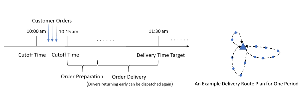
Appendix C Constraints for
Let be the travel time from location to location , be the on-site service time, and be a non-negative variable that records the delivery time of order by vehicle . The following constraints are added for (the dependence on is dropped below):
| (39) | ||||
| (40) |
where is a sufficiently large number. Constraints (39) ensure that if vehicle delivers order immediately after order , the delivery time of order should not be no earlier than the delivery time of order plus the travel time and the service time of order . Constraints (40) guarantee the delivery time of any order is no later than the target.
Appendix D Main Proofs
Proof D.1
Proof of Lemma 4.1 (i) We prove the first part by induction. For the last period (), is nondecreasing in because for . Now assume is nondecreasing in for . Then for any given , is nondecreasing in , and so is nondecreasing in by induction. It follows that the objective function of (7) is nondecreasing in (the expectation preserves the monotonicity). Therefore, is nondecreasing in by the property of , finishing the inductive proof.
(ii) The second part follows from the fact that the feasible region of APT is nonincreasing in . \halmos
Proof D.2
Proof of Theorem 4.2 (1) Lower bound. We can set for and for . This implies that drivers will be able to return to the depot within one period of their dispatch. Therefore, under this set of , we have a system wherein all the drivers are available at the beginning of every period, which is clearly a lower bounding system. More specifically, the optimal solution to APT would satisfy , of which the objective value will be less or equal to by the definition of .
(2) Upper bound. By the existence assumption, we can find a feasible myopic policy that dispatches drivers in period regardless of the realization of . Then we can choose the values of such that the optimal solution to APT is , and the optimal objective value is the same as the expected cost of (one such choice is to set and for ). Because is a feasible policy and its expected cost will be an upper bound of .
Lastly, when , we have
which is the same as problem APT because . \halmos
Proof D.3
Proof D.4
Proof of Proposition 4.4 When there exists a static myopic policy, APT is feasible with so is finite. Let define
| (41) |
We now prove that there exist satisfying and , such that
- 1.
: we can choose a large enough such that it is possible to dispatch drivers in every period (recall is the maximum number of customer locations), which yields the best possible on-time performance and thus is less than .
- 2.
: for period , there exists a lower bound such that is only finite when . Now we construct by setting . By doing so the only feasible solution to problem (41) is (from the property that is a non-decreasing function). As a result, , which is greater than the cost of any feasible static myopic policy because . Consequently, .
Next, let , then we have
because . Lastly, when is large enough for , the optimal dispatching and routing policy would be setting in every state, i.e., each driver will serve at most one customer location, which corresponds to the best achievable static myopic policy. As such .\halmos
Proof D.5
Proof of Theorem 4.5 We first focus on a single period with customer locations. As done in the proof of Proposition 4.4, the shortest expected delivery time is achieved when we can dispatch drivers so each driver only serves one customer. As such, the expected delivery time is per order. This is the lower bound of the single-period expected delivery time for customer orders, and we denote it by .
Due to the capacity constraint (and the possible delivery deadline), the number of dispatched drivers is at least . Now we provide an upper bound for the expected delivery time when dispatching drivers. The routing policy follows the well known tour partitioning scheme proposed by Haimovich and Rinnooy Kan 1985. Under this scheme, we first construct the optimal tour (TSP tour, ) through all the customer locations. Then we split the tour into segments and create feasible driver tours by connecting the depot with the endpoints of the segments.
Conditioning on the locations of the customers, there are ways to partition the optimal tour, each corresponding to a different starting location. Among the different partitions, a customer location will be connected to the depot (as the first visit location) times. When location is selected as the first visit location, the radial travel time will contribute at most to the delivery time of orders on the tour starting at (recall that a driver tour contains orders). Summing over the possible partitions, the total contribution from radial travel time is . Next we compute the contribution from the TSP travel time. For a given arc on the tour, , its contribution to the total delivery time depends on the delivery sequence of on the driver tour. When is the th visited customer on the tour, arc will contribute to the total delivery time (the customers following all include as part of their delivery time). Because can take values from to ( indicates is not on any driver tours, i.e., and are connecting to the depot), the total contribution from the TSP travel time over all the possible partitions is
where is the TSP tour length through the locations. Following a similar argument, the total contribution from on-site service time is for each partition. Therefore, the total delivery time of customer orders summing over the different partitions is
With a randomly selected partitioning, the expected delivery time would be
where we utilize the relationship . Then we take expectation with respect to the random locations of customers and derive the expected delivery time as
Because the above tour partitioning policy does not necessarily minimize the expected delivery time and only obtains a feasible solution, it provides an upper bound of the expected delivery time for a period with customer locations, . Then we have
The Beardwood-Halton-Hammersley (BHH) theorem implies that for large
where is the TSP constant (Beardwood et al. 1959). Hence, we can obtain an approximation for as
Now we consider the original expression of , which follows
where the expectation is taken with respect to the number of customer locations. Because we assume each customer orders exactly one item, the order quantity information is redundant and removed from the single-period optimal delivery time function. Moreover, observing that is decreasing in , we have
due to the assumption that for any . It follows that
which holds for large . \halmos
Appendix E Logic Benders Decomposition
The pseudocode of the logic Benders decomposition is presented in Algorithm 1. In this algorithm, is the tolerance of the optimality gap, and () is the best lower bound (upper bound) found by the algorithm. Let , and be the optimal costs of problems SF1, DF1 and F2, respectively. In each iteration, the algorithm first solves problem F2 and then solves problem RF1. Depending on the results, different types of Benders cuts are added to problem F2 to cut off the incumbent solution. If RF1 is infeasible, it indicates that the feasibility cut (30) is able to cut off the incumbent solution. If is greater than or equal to , it indicates that the optimality cut (29) is able to cut off the incumbent solution. Otherwise, the logic Benders cut (31) is used, and problem SF1 is solved exactly to update the best upper bound. The algorithm continues until the optimality gap is smaller than or equal to the given threshold.
Appendix F Label-Setting Algorithm
F.1 Basic Components
Because the reduced cost of a route is influenced by the time periods it goes through, the routes can be divided into different classes according to the period when a route returns back to the depot. Each class of routes correspond to a pricing problem. Now consider the pricing problem with respect to routes which must return back to the depot no later than period . Let be the maximum duration of the routes. Each pair of locations and is associated with a cost as follows:
| (42) |
Label Definition. Let be a label representing a partial path from depot to location where
- •
is the reduced cost of the path;
- •
is the earliest arrival time at location ;
- •
is the total demand of the visited locations;
- •
is the set of locations that the path can extend to.
Extension functions. The extension starts with an initial label . For a pair of locations and and a label associated with location , label can be extended to location to create a new label by the following extension functions:
| (43) | ||||
| (44) | ||||
| (45) | ||||
| (46) |
where is the demand of order and is the vehicle capacity.
Dominance rules. Let and be two labels associated with location . Then dominates if they satisfy the following conditions:
| (47) | ||||
| (48) | ||||
| (49) | ||||
| (50) |
The dominated labels can be safely discarded during the label extension to speed up the algorithm.
F.2 Bounded Bidirectional Search
Bounded bidirectional search partitions the extension of the label-setting algorithm into the forward extension and the backward extension according to the consumption of a chosen critical resource. In the forward extension, labels are extended in the same way as the original algorithm, while in the backward extension, labels are extended in the reverse direction. After both the forward extension and the backward extension finish, the resulted forward labels and the backward labels join together to generate the complete feasible routes, from which an optimal route can be extracted. Because the number of labels generated usually increases exponentially with the consumption of the critical resource, bounded bidirectional search has the potential to reduce the number of labels generated so as to speed up the algorithm.
Label Definition. Let be a backward label associated with location which represents a partial path from location to the depot, where
- •
is the reduced cost of the path;
- •
is the latest arrival time at locations ;
- •
is the number of locations visited in the path;
- •
is the total demand of the visited locations;
- •
is the set of locations that the path can extend to.
Extension functions. The backward extension starts with an initial label . For a pair locations and and a label associated with location , label can be extended to location to create a new label by the following extension functions:
| (51) | ||||
| (52) | ||||
| (53) | ||||
| (54) | ||||
| (55) |
Dominance rules. Let and be two labels associated with location . Then dominates if they satisfy the following conditions:
| (56) | ||||
| (57) | ||||
| (58) | ||||
| (59) | ||||
| (60) |
Label Combination. For a forward label and a backward label associated with location , they can be joined together to generate a feasible route if
| (61) | ||||
| (62) | ||||
| (63) |
where and be the set of locations visited by labels and , respectively. Conditions (61), (62) and (63) guarantee the satisfaction of the elementary constraint, the capacity constraint and the duration constraint, respectively. The reduced cost of the resulted route is equal to .
Critical resource. The duration is chosen as the critical resource. The break point of the forward extension and the backward extension is determined dynamically as follow. Let and be the upper limits of the critical resource consumption for the forward extension and the backward extension, respectively. That is, for a forward label , if , it will not be extended anymore. Similarly, a backward label will not be extended if . Let . Initially, and . The forward extension and the backward extension are executed. If the number of forward labels is greater than that of the backward extension, remains unchanged and is updated to . Otherwise, is updated to and remains unchanged. This process repeats until .
F.3 Ng-route Relaxation
The ng-routes are non-elementary routes first introduced by Baldacci et al. 2011. To each location , we associate a set of locations called ng-set, e.g. including the closest locations to location . Consider a path , if and , the path is referred to as an ng-cycle. A route is an ng-route if it does not contain any ng-cycles. The complexity of the pricing problem based on the ng-route relaxation and the quality of the obtained primal lower bounds depend on the size of the ng-sets. The larger the size of the ng-sets, the better are the lower bounds, but the more difficult it is to solve the pricing problem. Note that if , the pricing problem is equivalent to the ESPPRC, and if , the pricing problem is equivalent to the non-elementary SPPRC. Martinelli et al. 2014 propose an iterative approach to speed up label-setting algorithms based on the ng-route relaxation. First, the elementary constraint is relaxed, and each location is initialized with a small ng-set. Then the label-setting algorithm is called to determine the optimal ng-route. If the optimal ng-route does not contain any ng-cycles, it is elementary and optimal for the original pricing problem. Otherwise the ng-sets of the nodes in the ng-cycles are enlarged to forbid the ng-cycles, and the label-setting algorithm is called again. This process is repeated until an elementary optimal route is found. To handle the ng-route relaxation, the extension functions (46) and (55) are modified as follows:
| (64) | ||||
| (65) |
where .
F.4 Label Pruning
Label pruning is conducted during the extension phase in attempt to identify and drop the labels which cannot be extended to complete routes with negative reduced costs. Let be the minimum reduced cost of the partial routes from the depot to location with arrival time no later than . Then can be computed by the following dynamic programming:
| (66) |
Let be the minimum reduced cost of the partial routes from location to the depot with the number of the visited locations equal to . Then can be computed by the following dynamic programming:
| (67) |
The label pruning is done based on and . A forward label can be pruned if
| (68) |
where is the number of locations visited by . Similarly, a backward label can be pruned if
| (69) |
F.5 Label-Setting Algorithm for the Part-Time Drivers
The label-setting algorithm for the full-time drivers can be applied to the part-time drivers with following slight modifications.
- •
The trip duration is set to .
- •
The cost of locations pair and is set as follows:
(70) - •
Extension function (44) is replaced by the following function:
(71) - •
Initial backward extension label is initialized as .
- •
Dynamic programming (67) is modified as follows:
(72) - •
Condition (68) is modified as follows:
(73)
Appendix G Route Enumeration Algorithm
Proof G.1
Proof of Lemma 5.1 For a route , let denote problem SF1 where the constraints and the set of feasible routes are restricted to the nodes in , and be the optimal cost of problem . Given an upper bound of problem SF1 and a route , can not be in any optimal solutions of problem SF1 if it satisfies the following condition:
| (74) |
It is costly to check condition (74) because a VRP has to be solved for each route. Therefore, we use a lower bound of problem instead. Let and be the set of feasible routes which cover locations only in . A valid lower bound is the LP relaxation of problem defined as:
| (75) | ||||
| (76) | ||||
| (77) | ||||
| (78) | ||||
| (79) |
Let be an dual optimal solution of problem RF1. Then is a dual feasible solution of problem , and hence is valid lower bound of . If we replace this lower bound in condition (74), we have
| (80) | ||||
| (81) |
The label-setting algorithm introduced in Section F is used to enumerate the target routes by replacing the dominance rules (50) and (60) by the following dominance rules:
| (82) | ||||
| (83) |
The intuition of dominance rules (82) and (83) are that two labels cannot dominate each other if the corresponding paths of the labels do not visit the same locations. This ensures all feasible routes can be enumerated. Meanwhile, the ng-route relaxation is not used to speed up the label-setting algorithm. The detailed pseudocode of the route enumeration algorithm is summarized in Algorithm 2.
Appendix H Temporal Demand Distribution for Synthetic Instances
The following figures present the number of potential customer locations as a function of period for and , which controls the temporal variability in generating the synthetic instances.
Appendix I Additional Numerical Results for AJRP
We compare AJRP to two additional heuristic policies based on driver travel time minimization: (i) MinTravel_1: the dispatching and routing decisions are obtained by minimizing the total driver time (including return trip to the depot) while satisfying the hard deadline constraints for each epoch; (ii): MinTravel_2: this is similar to MinTravel_2 except that the return trip time is excluded in the objective function. These two heuristics, although myopic, tend to reserve vehicles for future deliveries. Figure 12 presents the performance comparison results of AJRP versus these two heuristics on the real data set. We observe AJRP outperforms MinTravel_1 and MinTravel_2 consistently by a large margin. This performance gap shows that minimizing driver time is not fully aligned with the system objective: to achieve faster deliveries for realized orders while maintaining a sufficient capacity for future deliveries. Specifically, these two heuristics dispatch too few drivers even when the capacity is not severely constrained.
Appendix J Detailed Computational Results on the MTRP Instances
This section presents the detailed computational results of our route enumeration algorithm on public MTRP instances against the state-of-the-art benchmarks. We observe that the proposed algorithm reduces the solution time substantially, yielding more than 60% improvement over the benchmarks in many cases. In addition, we implement a branch-and-price algorithm to solve problem SF1. The branch-and-price algorithm uses two types of branching rules in a hierarchy. First, if the number of routes in the optimal solution is fractional, the algorithm branches on the number of routes. Otherwise, the algorithm selects the arc with the most fractional value and branches on the selected arc.
[t]
| Name | Number of Customers | Route Enumeration Algorithm | Nucamendi-Guillén et al. 2016 | Muritiba et al. 2021 | |||||
|---|---|---|---|---|---|---|---|---|---|
| Cost | Time | Route Number | Time | Time | |||||
| brd14051 | 30 | 85729.72 | 0.88 | 746 | 4.66 | 9.41 | |||
| d15112 | 30 | 229130.8 | 0.86 | 682 | 9.58 | 3.67 | |||
| d18512 | 30 | 84818.95 | 0.77 | 584 | 6.85 | 2.64 | |||
| fnl4461 | 30 | 48287.5 | 0.43 | 760 | 2.83 | 3.65 | |||
| nrw1379 | 30 | 29994.97 | 0.80 | 795 | 5.83 | 9.9 | |||
| pr1002 | 30 | 164763.9 | 0.62 | 1017 | 8.09 | 4.76 | |||
| brd14051 | 40 | 106145.5 | 1.16 | 1130 | 30.37 | 43.49 | |||
| d15112 | 40 | 290748.6 | 1.78 | 1025 | 24.96 | 4.88 | |||
| d18512 | 40 | 107813.4 | 0.89 | 1322 | 11.74 | 8.21 | |||
| fnl4461 | 40 | 62672.49 | 0.76 | 967 | 17.21 | 21.92 | |||
| nrw1379 | 40 | 36379.77 | 1.04 | 1775 | 20.66 | 12.54 | |||
| pr1002 | 40 | 217071.6 | 1.15 | 1615 | 52.12 | 41.26 | |||
| brd14051 | 50 | 127480.6 | 1.85 | 1660 | 51.54 | 73.29 | |||
| d15112 | 50 | 356433.9 | 3.29 | 2715 | 53.75 | 33.37 | |||
| d18512 | 50 | 132115.4 | 1.65 | 1466 | 75.64 | 49.13 | |||
| fnl4461 | 50 | 76642.75 | 1.28 | 1216 | 32.11 | 20.14 | |||
| nrw1379 | 50 | 45169.23 | 1.89 | 5563 | 79.66 | 189.44 | |||
| pr1002 | 50 | 268605.3 | 2.61 | 1651 | 60.7 | 36.73 | |||
[t]
| Name | Route Enumeration Algorithm | Nucamendi-Guillén et al. 2016 | Muritiba et al. 2021 | |||||
|---|---|---|---|---|---|---|---|---|
| Cost | Time | Route Number | Time | Time | ||||
| E-n22-k4 | 819.39 | 1.42 | 106 | 4.90 | 4.32 | |||
| E-n23-k3 | 1555.87 | 3.01 | 1695 | 9.23 | 1.37 | |||
| E-n30-k3 | 1871.08 | 26.63 | 6621 | 119.11 | 1100.84 | |||
| E-n30-k4 | 1643.30 | 2.80 | 1023 | 22.95 | 301.07 | |||
| E-n33-k4 | 2819.43 | 5.43 | 1890 | 24.29 | 414.74 | |||
| E-n51-k5 | 2209.64 | 29.39 | 6127 | 2347.51 | t. lim. | |||
| E-n76-k7 | 2945.25 | 1075.67 | 545451 | - | t. lim. | |||
| E-n76-k8 | 2677.39 | 152.05 | 81838 | - | t. lim. | |||
| E-n76-k10 | 2310.09 | 38.19 | 5964 | 1700.64 | 2797.17 | |||
| E-n76-k14 | 2005.40 | 19.59 | 5816 | 236.64 | 271.04 | |||
| E-n76-k15 | 1962.47 | 18.40 | 5573 | 105.43 | 109.30 | |||
| E-n101-k14 | 2922.82 | 152.63 | 36952 | - | t. lim. | |||
- •
- means the corresponding instance was not tested.
- •
t. lim. means the computational time reached the time limit.
[t]
| Name | Route Enumeration Algorithm | Nucamendi-Guillén et al. 2016 | Muritiba et al. 2021 | |||||
|---|---|---|---|---|---|---|---|---|
| Cost | Time | Route Number | Time | Time | ||||
| P-n16-k8 | 382.90 | 0.46 | 803 | 1.90 | 0.36 | |||
| P-n19-k2 | 812.15 | 2.20 | 1711 | 9.13 | 1.27 | |||
| P-n20-k2 | 905.19 | 2.29 | 1759 | 11.60 | 2.07 | |||
| P-n21-k2 | 937.10 | 4.23 | 1663 | 11.07 | 6.36 | |||
| P-n22-k2 | 993.10 | 3.69 | 2067 | 11.00 | 1.87 | |||
| P-n22-k8 | 623.40 | 0.72 | 1147 | 3.08 | 0.29 | |||
| P-n23-k8 | 561.33 | 0.78 | 1328 | 2.68 | 0.29 | |||
| P-n40-k5 | 1537.79 | 9.30 | 1183 | 213.28 | 196.62 | |||
| P-n45-k5 | 1912.31 | 18.12 | 2109 | 495.82 | 3179.19 | |||
| P-n50-k7 | 1547.89 | 10.45 | 1766 | 117.48 | 211.15 | |||
| P-n50-k8 | 1448.92 | 8.62 | 1534 | 185.76 | 958.75 | |||
| P-n50-k10 | 1296.48 | 5.86 | 1724 | 112.32 | 13.57 | |||
| P-n51-k10 | 1419.43 | 6.32 | 2062 | 84.17 | 82.91 | |||
| P-n55-k7 | 1766.56 | 16.60 | 2068 | 790.31 | 3033.76 | |||
| P-n55-k8 | 1614.61 | 13.99 | 8909 | 170.89 | 136.19 | |||
| P-n55-k10 | 1438.60 | 7.86 | 5961 | 117.69 | 15.53 | |||
| P-n55-k15 | 1280.92 | 5.83 | 1678 | 48.01 | 4.23 | |||
| P-n60-k10 | 1676.35 | 12.45 | 2723 | 620.81 | 674.62 | |||
| P-n60-k15 | 1462.50 | 7.35 | 2247 | - | 13.14 | |||
| P-n65-k10 | 1928.46 | 17.91 | 2566 | 915.83 | 6762.68 | |||
| P-n70-k10 | 2097.17 | 22.35 | 3942 | 1415.78 | 5877.93 | |||
| P-n76-k4 | - | t. lim. | 297700 | t. lim. | t. lim. | |||
| P-n76-k5 | - | t. lim. | 129279 | t. lim. | t. lim. | |||
- •
- means the corresponding instance was not tested.
- •
t. lim. means the computational time reached the time limit.
Table 8 compares the computational performance between the route enumeration algorithm and the branch-and-price algorithm. We observe that the route enumeration algorithm outperforms the branch-and-price algorithm consistently. The main reason is that the branch-and-price algorithm has to explore a number of nodes to finally achieve the optimal solution.
| Class | Total Instances | Route Enumeration Algorithm | Branch-and-Price | ||||
| Instances | Average Time | Instances | Average Time | Number of | |||
| Tested/Solved | (In seconds) | Tested/Solved | (In seconds) | nodes | |||
| LQL | 180 | 180/180 | 1.32 | 180/180 | 22.86 | 17.6 | |
| E | 12 | 12/12 | 127.10 | 12/9 | 496.43 | 24.11 | |
| P | 23 | 23/21 | 8.45 | 23/21 | 276.08 | 20.80 | |