Non-Axisymmetric Precession of Magnetars and Fast Radio Bursts
Abstract
The repeating FRBs 180916.J0158 and 121102 are visible during periodically-occuring windows in time. We consider the constraints on internal magnetic fields and geometry if the cyclical behavior observed for FRB 180916.J0158 and FRB 121102 is due to precession of magnetars. In order to frustrate vortex line pinning we argue that internal magnetic fields must be stronger than about Gauss, which is large enough to prevent superconductivity in the core and destroy the crustal lattice structure. We conjecture that the magnetic field inside precessing magnetars has three components, (1) a dipole component with characteristic strength ; (2) a toroidal component with characteristic strength which only occupies a modest fraction of the stellar volume; and (3) a disordered field with characteristic strength . The disordered field is primarily responsible for permitting precession, which stops once this field component decays away, which we conjecture happens after years. Conceivably, as the disordered component damps bursting activity diminishes and eventually ceases. We model the quadrupolar magnetic distortion of the star, which is due to its ordered components primarily, as triaxial and very likely prolate. We address the question of whether or not the spin frequency ought to be detectable for precessing, bursting magnetars by constructing a specific model in which bursts happen randomly in time with random directions distributed in or between cones relative to a single symmetry axis. Within the context of these specific models, we find that there are precession geometries for which detecting the spin frequency is very unlikely.
Keywords:
stars: neutron — stars: magnetars — Fast Radio Bursts: FRB 121102 — Fast Radio Bursts: FRB 180916I Introduction
The relatively long 16.4 day period of FRB 180916.J0158 (Chime/Frb Collaboration et al. 2020) and the even longer 160 day period of FRB 121102 (Cruces et al. 2021, e.g.) suggest precession of magnetars deformed by strong internal magnetic fields (Levin et al. 2020; Zanazzi & Lai 2020). However, to date no evidence for a spin period has been reported for either of these FRBs (Zhang et al. 2018; Li et al. 2021, e.g.). One possibility is that not enough bursts have been detected yet for either FRB to reveal their spin frequencies, presuming that the underlying engine is a magnetar. But a second possibility is that the physical nature of the repeating busts might prevent detecting a spin frequency even in upcoming surveys that detect far larger numbers of individual outbursts.
The important phenomenological questions motivating this paper are:
- 1.
Should the spin period be detectable in FRBs that reappear periodically because of precession ?
- 2.
Is it possible for there to be no evidence for either a spin period or a precession period for FRBs associated with a precessing magnetar ?
Recently, evidence for a short second period has been presented by The CHIME/FRB Collaboration et al. 2021 from analysis of the light curve of a single outburst lasting seconds. This report lends urgency to addressing these two questions, and raises other issues we shall not address here, such as whether or not the 0.2 second period is due to magnetar spin, and, if it is, what the implications are for spindown, internal magnetic fields and precession.
In order to address these two questions, we first examine what the detection of precession tells us about the internal magnetic fields of the magnetars presumed to be the sources of the FRBs. Shaham 1977 showed that the pinning of (crustal) superfluid neutron vortex lines can prevent slow precession, and Link 2003 showed that pinning of neutron vortices to flux tubes associated with proton superconductor is likely wherever superfluid and superconductor coexist in the core of a neutron star. Moreover, for a neutron star rotating with period and precessing with period the moment of inertia of the region where neutron vortices are pinned must be times the total moment of inertia of the star for slow precession to be possible. We can’t rule out that FRB 121102 and FRB 180916.J0158 are both fine-tuned to the accuracy necessary to permit slow precession. However, we regard it as far likelier that the magnetic fields in the interiors of these magnetars are large enough to destroy proton superconductivity (and perhaps even neutron superfluidity).
§II.1 is devoted to discussing constraints on the internal magnetic fields that would be consistent with precession. We propose a specific model for the magnetic field that has three distinct components: in order of typical magnetic field strength these are a dipole field, a toroidal field, both of which are ordered, and a disordered field. We develop this model in §II.2, where we are led inevitably to the conclusion that the quadrupole distortion of the star is triaxial, and most likely somewhat prolate. We also propose that a magnetar may only precess for a relatively short portion of its life lasting perhaps 1000 years.
§II.3 develops results on triaxial precession necessary for the more phenomenological modelling done in §III. In particular, we show that rather large amplitude precession can be excited with relatively little fractional expenditure of magnetic energy, a natural consequence of the fact that magnetic energy is sustantially larger than rotational energy in magnetars. We also consider two distinct types of effects due to spindown. In §II.4 we develop the timing model relating observer time to precession phase when spindown is included. There are two effects, the familiar long term spindown but also a cyclical effect specific to precessing pulsars that has period (Cordes 1993). In §II.5 we investigate the secular effect of spindown on the precession amplitude and phase, generalizing work done by Goldreich 1970 for oblate axisymmetric precession to triaxial precession. We outline a simple phase diagram for this more complicated problem that is more complex than what arises for oblate, axisymmetric precession.
Finally, in §III we develop a very specific model in which we assume that FRBs are tied to magnetar outbursts that occur randomly in time and point in random directions about some reference axis, which we take to be (but need not be) the magnetic dipole axis. We show that it is impossible to detect either the spin frequency or the precession period if the outbursts can point in any direction, which is not a big surprise. However, we also find that the spin frequency ought to be easy to detect in some cases and much harder in others, depending on specific characteristics of the precession model and the distribution of beam directions of the outbursts.
From a qualitative point of view, we offer two simple reasons that the outbursts underlying FRBs may occur randomly in time. Although tautological, one explanation is that the physical mechanism triggering the bursts simply is stochastic temporally, with burst directions that are random within some boundaries. Another is that the times between burst triggers are irregular but correlated, perhaps because there is a characteristic time for the burst phenomenon to reload, but associated with each outburst is a random time offset, possibly as large as the spin period, related to where the burst is triggered within the magnetar magnetosphere. The bursts may point in a large range of directions because they involve plasma moving relativistically along open magnetic field lines, leading to highly focussed energy output in directions ranging from close to the magnetic dipole axis to perpendicular to the light cylinder. Alternatively, bursts may originate from a set of distinct, concentrated regions in the magnetosphere of a magnetar that turn on and off stochastically, with each region beaming energy outward in a different direction.
In a companion paper we address the challenge of uncovering an underlying FRB spin frequency in a more general, phenomenological way that does not rely on as specific a model for bursts from rotating magnetars as we develop in §III. The model presented in this paper can be regarded as a definite physical set up that realizes the general conditions for hiding the spin frequency of an FRB-inducing magnetar developed in the companion paper.
II Internal Magnetic Fields and Triaxial Precession
II.1 Internal Magnetic Fields that Permit Slow Precession
Previous work has focussed primarily on precession arising from oblate axisymmetric distortion due to magnetic stresses (Levin et al. 2020; Zanazzi & Lai 2020, e.g.). Here, we examine what internal magnetic structure may be required for precession to occur, and highlight distinctive features that arise when the distortion is not axisymmetric and possibly prolate.
The internal magnetic structure of magnetars is not well-studied. In general, magnetohydrodynamic (MHD) studies of the magnetic fields in normal conductors have shown that there are no stable magnetic field configurations in barotropic normal fluids (Lander & Jones 2012; Mitchell et al. 2015), but that stable, axisymmetric configurations may exist in stably stratified fluids (Reisenegger 2009; Akgün et al. 2013; Mitchell et al. 2015). Braithwaite 2009 and Akgün et al. 2013 argued that there may be stable magnetic field configurations in stably stratified stars whose poloidal fields are much weaker than their toroidal fields. Glampedakis & Lasky 2016 argued that the equilibrium magnetic fields in non-barotropic normal fluid stars can be specified freely if they are axisymmetric, but not if they are non-axisymmetric. At the strong fields we envision, magnetization due to Landau quantization of core electrons also affects stability (Rau & Wasserman 2021; Suh & Mathews 2010). Relativistic equilibria have been computed using realistic equations of state (Cardall et al. 2001; Kiuchi & Yoshida 2008; Frieben & Rezzolla 2012, e.g.); equilibria were only found to exist if the maximum internal magnetic field strength is G, which is a significant indication of limitations imposed by overall dynamical stability, but does not assess MHD stability. Of course, stability constraints are not necessarily relevant if the magnetic field is time-dependent, although presumably field configurations that are MHD unstable vary rather rapidly on timescales set by the local Alfvèn speed and the lengthscale of variation.
Overall, these studies suggest that the internal magnetic fields of magnetars could be considerably stronger than their dipole (surface) magnetic field.
Another, rather different, argument also suggests strong internal magnetic fields. Once the core of the star cools below core protons become superconducting unless the internal magnetic field is stronger than the second critical field strength
| (1) |
where is the proton gap, is the proton Fermi momentum, is the proton effective mass, is the coherence length and is the flux quantum. Proton gap calculations are complicated by many body effects at high densities (Zuo et al. 2008; Gezerlis et al. 2014; Dong et al. 2017; Guo et al. 2019) but indicate that near nuclear density , where ; decreases to zero at densities . Of course, it is also possible that protons are superconducting but magnetic field strengths at the inner boundary of the (normal) crust are below the first critical field strength
in which case magnetic fields would not penetrate into the superconductor in equilibrium if entering from the outside. However, very likely magnetic flux in the core is “left over” from before it cooled enough to become superconducting (Baym et al. 1969, e.g.), in which case the proton superconductor in the core is in a “mixed state” with . Quadrupolar deformations due to magnetic fields are
| (2) |
for magnetic induction Gauss, stellar radius km and mass , where for a normal conductor but for a type ii superconductor (Jones 1975; Cutler 2002; Wasserman 2003; Henriksson & Wasserman 2013; Akgün & Wasserman 2008, e.g). The parameter depends on the structure of the neutron star and of its internal magnetic field, and represents how effectively the magnetic forces cause quadrupolar deformation.
The superconductor is type ii as long as , which is the case throughout much of the region where protons are superconducting. In a type ii superconductor, magnetic flux is organized into an array of thin flux tubes that have an areal density . If the neutrons are also superfluid their vorticity would be confined into thin vortex lines with a much lower areal density for a rotation period seconds, where is the neutron chemical potential in units of the neutron rest mass. Unless the relative velocity between flux lines and vortex lines is big enough, which may be true if the precession amplitude remains sufficiently large (Link & Cutler 2002), vortex lines will pin to flux lines (Link 2003), which frustrates slow precession (Shaham 1977). This problem can be avoided entirely if the core of the neutron star is hot enough that neutrons remain normal: neutron gaps are (Zuo et al. 2008; Gezerlis et al. 2014; Dong et al. 2017; Guo et al. 2019). Calculations by Potekhin & Chabrier 2018 indicate that the core of a magnetar may cool below within years of forming, so neutrons may be normal in some but not all of the core of a year old magnetar unless the maximum neutron critical temperature in the core is lower than current estimates. But even a moderately small region where protons and neutrons are both superfluid could have an important impact on neutron star precession: for a precession period days the moment of inertia of any region in the core where vortices are pinned to proton flux tubes must be times the total moment of inertia of the star (Shaham 1977).
Here, we assume that the magnetic field in the core is strong enough to suppress superconductivity entirely. This means that we suppose that the total magnetic field strength throughout all of the core. For this to be true, the internal field strength must be at least comparable to and probably larger than the dipole magnetic field at the stellar surface. This may be achieved if there are substantial non-dipolar components of the internal magnetic field, particularly toroidal components (Cutler 2002, e.g.). Akgün et al. 2013 found stable, axisymmetric equilibria with toroidal fields times stronger than the poloidal fields. The deformation due to toroidal fields can be axisymmetric, but if so is prolate rather than oblate.
Vortex line pinning may also be a problem in the neutron star crust, where neutron pairing is S-wave and superfluid gaps are larger, (Gezerlis et al. 2014); neutrons are likely to be superfluid down to densities close to neutron drip for temperatures K (Potekhin & Chabrier 2018). Unpinning and repinning of neutron superfluid vortices to crustal nuclei have long been thought to be responsible for the behavior of pulsar spins during and after rotational glitches (Anderson & Itoh 1975; Anderson et al. 1982; Alpar et al. 1984; Link et al. 1993). Strong magnetic fields alter the equation of state because the degenerate electron gas becomes one dimensional once
the equation of state of the inner crust is largely unaffected for Gauss, although it stiffens considerably in the outer crust (Mutafchieva et al. 2019). The crust ought to crystallize except at low densities for temperatures (Carreau et al. 2020). Neutron star precession can only persist in spite of potential pinning of neutron superfluid vortex lines to crustal nuclei or pasta phases (Ravenhall et al. 1983; Hashimoto et al. 1984; Lorenz et al. 1993) if the sustained precession amplitude is large enough (Link & Cutler 2002). The complex topology of the nuclear pasta revealed by molecular dynamics simulations (Schneider et al. 2018) could complicate pinning.
There are two other effects of superstrong crustal magnetic fields that should alter the physical conditions there, perhaps enabling precession to occur. One effect is to shatter the crystalline crust, which can happen if , where is the elastic shear modulus. Molecular dynamics simulations by Caplan et al. 2018 indicate that the shear modulus of nuclear pasta is , so crustal magnetic fields Gauss would shatter the crust. (See also Pethick & Potekhin 1998).
A second possibility presents itself for magnetic fields larger than the Clogston-Chandrasekhar limiting field strength (Clogston 1962; Chandrasekhar 1962)
| (3) |
above which flipping the spin of one neutron can break a S-wave Cooper pair; here is the neutron gap and is the neutron magnetic moment. For such large magnetic field strengths, the uniform S-wave BCS superfluid condensate transitions to an inhomogeneous LOFF state (Larkin & Ovchinnikov 1974; Fulde & Ferrell 1964; Kinnunen et al. 2018). Although the implications of such states in the crust have not been explored extensively, it is conceivable that the inhomogeneous LOFF state behaves more like a crystal than a (super)fluid, which may permit precession to occur (Lee et al. 2018). Moreover, somewhat weaker magnetic fields may destroy the predominantly P-wave superfluidity of core neutrons for which keV (Haskell & Sedrakian 2018, e.g.).
In any event, we conclude that magnetic fields stronger than about are necessary for slow precession. However, the precession period is of order
| (4) |
which, in view of Eq. (2), suggests a quadrupolar deformation corresponding to for FRB 121102 and FRB 180916.J0158+65, which is too weak to prevent superconductivity of core protons according to Eq. (1). We therefore propose that the magnetic fields inside these magnetars consist of three components:
- 1.
a dipole field with characteristic strength ;
- 2.
a quadurpolar field with characteristic strength and a symmetry axis misaligned with the dipole moment;
- 3.
a disordered magnetic field with characteristic strength strong enough to suppress superconductivity but with large scale stresses that do not contribute significantly to the quadrupolar deformation of the star.
The spindown timescale in this model is of order
| (5) |
where is the moment of inertia of the star and ; the expected ratio of spindown timescale to precession period is
| (6) |
so spindown is very slow compared with precession. Below, we shall also suggest that decays via ambipolar diffusion within years. That would mean that if FRB 121102 and FRB 180916.J0158+65 have they are both younger than their spindown ages and spinning close to their original rotational frequencies. However if they are spinning faster, with then they might be about as old as their spindown ages, have quadurpolar distortions , and be of order halfway through their lifetimes as precessing neutron stars.
II.2 Magnetic Precession
In this paper, we consider triaxial magnetic distortions that may be far from oblate. We shall see that such configurations lead to qualitatively new features for neutron star precession that may have distinctive observable consequences. Precession of a fluid star caused by magnetic distortions differs qualitatively from solid body precession even though mathematically the two are the same. The inevitability of precession for stars with non-aligned spin and magnetic fields was originally pointed out by Spitzer 1958, and was studied extensively by Mestel and collaborators (Mestel & Takhar 1972; Mestel et al. 1981; Nittmann & Wood 1981). These studies also found that there are slow, internal nonrigid motions in addition to uniform rotation which have been studied recently by Lander & Jones 2017 for neutron stars with toroidal magnetic fields. Below, we neglect these motions, which are second order in small quantities although we recognize that they may be significant for magnetic field evolution.
In a rotating, highly magnetic fluid the matter density is perturbed away from spherical symmetry. The moment of inertia tensor of the star only depends on the perturbations:
| (7) |
where rotation is along the direction, and are the amplitudes of the distortions due to rotation and magnetic fields, respectively, and is symmetric and trace free (STF). The stellar angular momentum is
| (8) |
where we use the summation convention. Since we ignore the difference between and below. Invert Eq. (8) to get to first order in small quantities. Since is STF
| (9) |
for an axisymmetric magnetic field but we regard this case as exceptional (although Spitzer 1958 and Mestel & Takhar 1972 and subsequent work focused on this situation). Since is fixed in the rotating frame of reference
| (10) |
in the inertial frame. If the star is axisymmetric, precession is about the magnetic field axis of symmetry, as is well-known (Spitzer 1958; Goldreich 1970; Mestel & Takhar 1972, e.g.), but this is untrue for the more general non-axisymmetric case, where precession is more complicated.
For the intense magnetic fields we envision, the main cause of quadrupolar deformations are magnetic stresses. Even in non-barotropic stars, the magnetic field configurations that give rise to static deformations are highly constrained (Glampedakis & Lasky 2016). In such a star, the static structure is perturbed away from spherical symmetry by the Lorentz force density ; to linear order
| (11) |
where is the gravitational acceleration in the unperturbed star, is the pressure perturbation. is due to non-fluid forces, and is the gravitational potential of the perturbation. In the neutron star core, where , axisymmetric static perturbations require that the toroidal field is
where is the flux function of the poloidal field
but for nonaxisymmetric fields (Glampedakis & Lasky 2016). Assuming that this restriction holds, Eq. (11) is easy to solve in a non-barotropic star, where and are unrelated.
Lasky & Melatos 2013 considered a specific example of a nonaxisymmetric field with dipole and toroidal fields that have different axes of symmetry and , respectively, that lead to static deformations of the star. Below, we use a slightly different model for the dipole and toroidal fields, and also include a disordered component. Assuming that the quadrupolar deformation due to the disordered component is relatively small, magnetic forces due to the ordered dipole and toroidal fields result in a perturbed moment of inertia tensor
| (12) |
Both and are positive, and it follows that the toroidal field promotes prolate deformations relative to a symmetry axis whereas the dipole field promotes oblate deformations relative to a symmetry axis . If we assume that
| (13) |
in a right-handed coordinate system then we find that the eigenvalues of are
| (14) |
where we have defined .
For the dipole field, we adopt a stream function
| (15) |
where the dimensionless function is
| (16) |
for a mass profile . The magnetic field matches smoothly to an exterior vacuum dipole provided that both and at the stellar surface. Typically, the poloidal magnetic field vanishes somewhere along its equator, and is prone to instability there. In the Cowling approximation we find that
| (17) |
independent of the detailed density profile of the star, but including self-gravity changes by a factor .
The toroidal field must vanish at the surface of the star in order to match to a vacuum exterior. (The toroidal fields in a pulsar magnetosphere are much weaker than the internal toroidal fields we consider here.) For in the neutron star core, this important constraint can be satisfied in two ways that lead to very different values of .
- 1.
The toroidal field may fill the core,
(18) and plunge to zero in a thin boundary region where may be nonzero, thus loosening constraints on , even if the crust is damaged severely by its strong magnetic field. The value of depends on the density profile; we adopt
(19) where is the moment of inertia of the spherical star; for this particular density profile including self gravity implies
(20) To zeroth order in the shell thickness
(21) for this model, where is the mean square toroidal field strength. The thin shell contributes about half of the deformation, which may be unrealistic, so actual values could be as small as half as large.
- 2.
The toroidal field may be confined to a limited valume if instead of Eq. (18)
(22) which is the model used by Lasky & Melatos 2013. (See also Akgün et al. 2013, who introduced models of this type in their study of magnetic stability in axisymmetry.) The field only occupies about 21% of the stellar volume, and has a mean square within this volume. In this case
(23) The quadrupole moment for this model is diminished severely because it is confined to such a small volume.
- 3.
Interpreting these two models as extremes for quadrupolar distortion due to toroidal fields we estimate
(24) and therefore
(25) Thus, and may even be ; the quadrupolar distortions arising from ordered field are significantly triaxial, and very likely prolate.
If the toroidal field occupies a small volume, as for Eq. (22), then no matter how large is the field will be incapable of suppressing proton superconductivity everywhere. Even if the field occupies much of the star, as in Eq. (18), it may not be strong enough to exceed even if it is much stronger than . Moreover, as noted above is prone to instability in this model. Although the toroidal field represented by Eq. (22) can prevent the instability in axisymmetry if is large enough (Akgün et al. 2013) we doubt that the tilted dipole model is stable ( for both Eqs. (22) and (18) in axisymmetry but not in the tilted dipole model.) For these reasons we conclude that a precessing neutron star with internal fields that are stable on short timescales ought to include a disordered component for with characteristic local field strength . The disordered field may be a remnant of the violent process that generated the strong internal magnetic fields (Thompson & Duncan 1993; Braithwaite 2009).
The turbulent magnetic field is
| (26) |
where the scalar functions are constant along field lines and are advected with the fluid in the limit of perfect conductivity. We can think of as a pair of comoving field line labels. We assume that the turbulence is small scale locally but with a large scale bias, so that we can expand
| (27) |
where is a spectral function and is the ratio of the small scale that characterizes the local turbulence and the large scale that characterizes the bias; is a normalization volume and is a random phase. If we assume that , which is plausible if the turbulent field results from fluid motions that stretch, twist and fold individual field lines, then Eq. (26) has a mean value times the characteristic local field amplitude, and there are magnetic forces (corresponding to gradient of turbulent magnetic pressure), and (corresponding to the mean field). We assume that the local field is strong enough to destroy superconductivity, but that the forces are too weak to have much effect on quadrupolar deformation. However, we do hope that the stresses can act as deus ex machina to stabilize the ordered fields.
Magnetic fields in the core of a highly magnetic neutron star containing normal neutrons and protons decay via ambipolar diffusion: Reisenegger & Goldreich 1992 estimate a decay timescale
| (28) |
for field varying on a length scale km, where is baryon density, is nuclear density, is the proton density, and . (See also Glampedakis et al. 2011, Passamonti et al. 2017 and Gusakov et al. 2017, Fig. 1.) Neutron superfluidity would increase the decay time but as long as the core temperature is as high as K the normal neutron fraction will be considerable in much of the core, and Eq. (28) remains true within a factor of an order of magnitude or less. (Field decay heats the core, but given the steep dependence of neutrino cooling the core temperature is not changed substantially.) The tangled component will decay on a timscale that depends on its fluctuation spectrum: if the decay timescale , which implies faster decay on smaller scales for and vice-versa; theories of fully developed magnetic turbulence generally find (Iroshnikov 1963; Kraichnan 1965; Goldreich & Sridhar 1995). Plausibly, the tangled field decays away in a time y, after which substantial portions of the magnetar core become superconducting, which limits the time span during which a magnetar may precess slowly. The larger scale ordered fields also decay as long as core protons are normal but since for these fields they may survive relatively undiminished until protons become superconducting, after which ambipolar diffusion becomes ineffective. Ambipolar diffusion in the crust is suppressed by neutron superfluidity. Magnetic field evolution in a magnetar crust involves an interplay among the Hall effect, Ohmic dissipation and plastic flow (Lander & Gourgouliatos 2019; Li et al. 2016), involving instabilities on timescales (Gourgouliatos & Pons 2020) and possibly evolution toward an attractor solution on timescales (Gourgouliatos & Cumming 2014b; Gourgouliatos & Cumming 2014a). (The effect of Landau quantization of crustal electrons on magnetar magnetic field evolution, which may be substantial, is being included for the first time in a forthcoming paper by Rau, P. B. & Wasserman 2021.)
II.3 Triaxial Precession
Conservation of angular momentum is
| (29) |
where is the angular momentum and is the spindown torque; is time derivative in rotating frame. Substitute where to get
| (30) |
and
| (31) |
For the spindown torque we adopt
| (32) |
where is the magnetic moment of the star, and are numerical constants ; for numerical evaluations we adopt and , which corresponds to a rate of energy loss where (Li et al. 2012). (The same spindown model was used in Akgün et al. 2006.) The angular velocity of rotation is
| (33) |
where are the moments of inertia along the principal axes of the quadrupolar distortion; we define a parameter , which measures the degree of triaxiality, in terms of which
| (34) |
where is given by Eq. (2). Oblate axisymmetric distortions () correspond to ; prolate axisymmetric distortions () correspond to . For the tilted dipole model (Lasky & Melatos 2013, see Eq. (14) and)
| (35) |
For the dipole field dominates the quadrupolar distortion and Eq. (35) implies that . For the toroidal field dominates the quadrupolar distortion, and Eq. (35) implies that . For , the axisymmetric case, if and for .
The Euler equations have an exact conservation law
| (36) |
because is a unit vector, but there is also an approximate conservation law
| (37) |
so only varies appreciably on a timescale of order times the spindown time. In Eq. (37) the parameter is the magnitude of the stellar angular momentum at some reference start time, which could be the time when precession is excited.
The Euler equations allow steady state rotation about any of its three principal axes. By combining Eqs. (36) and (37) in three different ways appropriate to perturbation away from each principal axis we find
| (38) |
Eq. (38) shows that at a given angular momentum, the lowest energy state is rotation about , the highest is rotation about and rotation about is intermediate, as is well-known. For axisymmetric oblate precession () the and directions are interchangeable, and precession about either one is unstable but stable about the symmetry axis , but for axisymmetric prolate precession () the and directions are interchangeable, and precession is stable about either one and unstable about the symmetry axis .
Below, we will use the first of Eqs. (38) to quantify the second conservation law by defining the energy perturbation above the minimum energy state to be
| (39) |
where is the extra energy associated with precession. Using Eq. (39) we write the conservation law as
| (40) |
Suppose precession is excited from its minimum energy state by injection of rotational energy . This is consistent with exciting precession with amplitude
| (41) |
There are then two very different cases depending on how much energy is injected: if then and if then . We shall treat each of these cases, which have very different properties, separately. Qualitatively, we shall see that has well defined (axisymmetric, oblate) limiting dynamics whereas has well defined (axisymmetric, prolate) limiting dynamics. Since
| (42) |
where is the magnetic energy and is the binding energy of the neutron star, a more apt comparison is
| (43) |
where is the rotational distortion of the star.
For a rotation period second we expect so the energy required to excite even high amplitude precession is only a small fraction of the magnetic energy of the star. Even small changes in the magnetic field can engender relatively large amplitude precession. To make this quantitative, suppose that a shearing event in the neutron star distorts the magnetic field changing the moment of inertia of the star from to , where is STF. The eigenvalues of are slightly different than those of , and its eigenvectors are rotated relative to the eigenvectors of . If the eigenvalues and associated eigenvectors of are , then to lowest order in the eigenvalues and eigenvectors of are
| (44) |
normalizing the eigenvectors so that . Since we expect , where is STF with magnitude , and the rotations involve angles , not . Assuming that is conserved in the shearing event, its projection along the rotated principal axes of differs from its projection along . For example, suppose that the star was rotating without any precession at all along , the axis of largest moment of inertia, prior to the shearing event; then afterwards
| (45) |
and the star will precess. If angular momentum is conserved as the field rearranges itself, then the angular velocity changes during the shearing event by
working in the reference frame where is diagonal. The associated change in rotational energy is
| (46) |
might be negative or positive, and is not equal to the extra energy in precession above the minimum energy state corresponding to rotation about , in part because the magnitude of the angular velocity changes as a result of the shearing event. In rough order of magnitude .
Phenomena associated with the spindown torque include a cyclical variation over a precession cycle and a secular torque that develops very slowly compared with the precession period. We discuss these in Sections II.4 and II.5 using a perturbative technique similar to Goldreich 1970 but generalized to triaxial precession. To zeroth order, we neglect spindown effects, and Eq. (31) becomes
| (47) |
where is differential spin phase.
From an observational standpoint, we are most interested in the motion of the direction from the star to the observer, , in the rotating frame of reference. In the inertial frame, where is independent of time to lowest order, let
| (48) |
To project into the rotating frame we use a standard Euler angle rotation (Gottfried 1966): (i) Rotate angle about the 3 axis to get new axes , (ii) Rotate angle about the axis to get new axes . (iii) Rotate angle about the axis to get the axes . In terms of the angles , and we get where
| (49) |
If we define in the inertial frame we find that and
| (50) |
Using for any of the principal axes we find that
| (51) |
using Eq. (40). Note that these results can be used for both and .
In the rotating frame of reference, where and are slowly varying unit vectors perpendicular to ; rotates rapidly in the retrograde direction in the plane instantaneously perpendicular to . For emission along a beam direction the observed intensity depends on
Define , and ; then
| (52) |
where and vary during the precession cycle for a given .
For “pulsar-like” behavior, beam directions are randomly distributed in a narrow cone around a dominant direction. Given unlimited sensitivity, the observed intensity would be nearly periodic, with periodic timing residuals due to precession radian of spin phase. The amplitude of the rapidly oscillating term in Eq. (52) is , which varies during the precession cycle. Presumably the observed intensity is a decreasing function of , so the observed intensity has extrema when
| (53) |
which has solutions twice per cycle, only one of which corresponds to the maximum value of . Intrinsic intensity fluctuations and imperfect, time-varying and often unfavorable beaming due to precession turn out to render most pulses undetectable, but nevertheless the spin frequency would be discernible readily in this case.
For “stochastic behavior” in which outbursts occur randomly in time with a random distribution of beam directions it is much harder but not impossible to uncover the pulse frequency. If the beams emit into narrow cones, Eq. (52) implies that most outbursts will not be seen but there will be a bias favoring times when is near one. This bias imprints the effect of fast rotation on the times when outbursts happen, but only weakly, so the spin frequency is only discernible after many bursts have been detected. We develop a specific model for stochastic outbursts in §III. An approximate analytic model that elucidates how information about the spin frequency and precession period is imprinted on the modelled series of burst detection times may be found in Appendix B.
Intermediate between these two extreme models would be one in which FRBs occur randomly in time but are triggered by exceptionally narrow beams within a restricted range of possible directions. For an outburst occuring at a particular time, the associated FRB would only be seen if is very nearly parallel to , as determined from Eqs. (49) with Eq. (50), and is in the range of allowed beam directions.
| 11 1 is required. | ||
| 22 2 Precession phase. and are elliptic functions (e.g. Abramowitz & Stegun 1972, ) | ||
| 33 3 Precession phase per precession cycle. | ||
| 44 4 Spin phase per precession cycle. | ||
| (Axisymmetric, Oblate) | (Axisymmetric, Prolate) | |
Table 1 details the solutions of the Euler equations. Note that the solutions are continuous across the limiting case , but because the precession period diverges logarithmically as (from either side) the solutions are not really connected physically across .
There are two different axisymmetric situations, , which is oblate (), and , which is prolate (); these solutions are listed in Table 1. However, these are singular limiting cases: is identically zero for and any value of and is infinity for for any value of .
The ratio of the neutron star spin period to its precession period is
| (54) |
which is plotted in Fig. 1 for various values of as a function of . The smallest values of are for and large , except for the region right around , where for all values of . Since R1 and R3 both have very long , Fig. 1 favors models with large values of , which implies that the toroidal component of magnetic field is significantly larger than the poloidal component, unless the star is fortuitously close to .
II.4 Periodic Timing Residuals from Precession Plus Spindown
Here, we derive the equation for , the functional dependence of time on spin phase, which we have defined previously as ; we use Eqs. 30 and 32 to zeroth order in to get
| (55) |
where and in this approximation. The solution to Eq. (55) is a continuous function that exhibits the timing residuals due to spindown; for a single beam, which is appropriate for a precessing pulsar, we evaluate at , the discrete set of spin phases where the pulses are beamed toward the observer optimally.
The dependence on precession phase arises from
| (56) |
where we used the conservation laws, Eqs. (36) and (40), to separate out the constant term and isolate the dependence on . In evaluating we must be careful to isolate secularly growing terms from terms that are periodic over a precession cycle. We write the solution to Eq. (55) succinctly as
| (57) |
where . Coefficents in Eq. (57) are given in Table 2. The various averages and functions in Table 2 are evaluated in Appendix A.
For calculations, it is convenient to express in terms of the precession period . Then and the remaining terms all depend on the single nondimensional parameter
| (58) |
because Eq. (55) may be written in the form
From Eq. (57) we see that in addition to the apparent frequency shift arising from precession there is another apparent frequency shift .
The amplitude of the cyclical terms is of order
| (59) |
and the cyclical shift in pulse phase due to spindown is of order
| (60) |
which can be large for
| (61) |
(Cordes 1993). The secular terms also become progressively more important for and, if large enough, may frustrate searches for the underlying spin period of the precessing magnetar in models based on stochastic outbursts. Eqs. (58) and (61) imply that
| (62) |
which is between and if (FRB 121102) and between and if (FRB 180916.J0158+65) for .
II.5 Secular Evolution of Precession via
We now consider how precession evolves as a consequence of spindown, generalizing Goldreich 1970 to cases with . As in Goldreich 1970 we consider effects to lowest order in . We generalize the solutions to the Euler equations to include slow evolution of the amplitude parameter , as was done by Goldreich 1970, but also include a slowly varying phase shift by replacing with . This phase shift is required for triaxial precession evolving via spindown. Here is roughly the inverse spindown time. We assume that the spindown time is long compared with the precession timescale, a necessary condition for a perturbative treatment; this assumption fails at early times, or if .
We start by considering , which is favored for long precession periods, and is the expected state if precession is excited from rotation about with relatively low . Averaging over precession phase we find
| (63) |
where we used
| (64) |
Eq. (63) reduces to the results in Goldreich (1970) for , the axisymmetric oblate case, for which and , after replacing using Eq. (64); for that case, there is no phase shift .The stability condition implied by the first of Eqs. (63) is more complicated than what was found by Goldreich (1970) for the axisymmetric, oblate case: there is a separatrix that is an ellipse in the plane whose axes depend on , so that, for given values of and and , there is a fixed point at a specific value of .
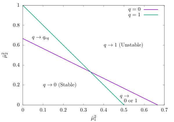
By contrast, for the axisymmetric oblate case, the ellipse degenerates into a circle
| (65) |
irrespective of the value of . In this case, grows as long as the magnetic moment configuration of the star is outside this circle. The growth halts once , where also goes to zero. Inside the circle, decreases, reaching asymptotically.
For the triaxial case cannot grow beyond ; since for , Eq. (63) implies . The stability curve (infinitesimally) close to is
| (66) |
The two curves intersect at ; in fact all of the stability boundaries intersect at this point since and . These two bounding stability lines are depicted in Fig. 2. The stability boundaries for all other values of are between these two lines, pivoting about their intersection point at .
Fig. 2 depicts evolution outcomes for various regions in the phase plane. The region marked “” is unconditionally unstable: if precession is excited for in this region, grows on the spindown timescale until , where growth ceases. Conversely, the region marked “” is unconditionally stable: if precession is excited for in this region, shrinks toward zero on the spindown timescale. In the two triangular regions between the and bounding curves at for each . In the region marked “,” for and for , so if precession is excited in this region asymptotically as a result of spindown. In the region marked “ or ”, for so asymptotically if precession is excited with and for so asymptotically if precession is excited with .
III Application to Fast Radio Bursts
III.1 A Random Burst Model
To this point, we have focussed on the combined effects of precession and spindown on observations of emission along a single beam in which emitted intensity is determined entirely by . For application to FRBs we develop a different model in which multiple beams pointing in random directions fire at random times with random intrinsic intensities.
To address these questions we simulate an ideal observing program consisting of daily observations over a total observing time lasting precession cycles. In our idealized observing campaign, each daily observation starts one day after the beginning of the previous one and lasts days (2.4 hours). We assume that bursts occur at a uniform rate throughout the duration of the observing program and that occur during the total time of the observations. We input in days, so that the number of observing days is the integer part of plus one.
We also input the parameters of the precession model, from which we can compute the spin frequency . We choose randomly in the range .
The simulation starts by choosing the set of individual burst precession phases; in the absence of spindown the corresponding burst times are , and even with spindown included the burst times only differ from these times by . For each simulation there are bursts. Ultimately, only a small fraction of these are detectable.
For each we next determine a beam direction in the rotating frame of reference. We do this relative to a reference beam whose direction we input. In the calculations presented here we assume that this reference direction coincides with the direction of the dipole moment appearing in the spindown formula, . We assume that is anywhere between two cones about defined by , adopting a uniform distribution for over this range and a uniform direction of azimuthal angles in . We could, of course, choose a different reference direction or multiple reference directions among which bursts may switch. As should already be apparent, there are many parameters in this model, and choosing a single reference direction simplifies the calculation somewhat. Our model does allow the reference direction to switch to a different one with a probability , but the results reported here are for .
The next step is to compute for each outburst. We do this by computing in the rotating frame of reference from Eq. (52). This requires choosing a value of the inclination angle defined in Eq. (48), which we input.
Once we have the value of for a given outburst we can decide whether or not that outburst is detectable. As a first cut, we discard all bursts for which since these point away from the observer. Because we assume that each beam has a FWHM we may be discarding some bursts that could be detectable, in principle, but as long as is not too large we expect that this is not an important source of inaccuracy in our conclusions. We do not discard beams that would be eclipsed by the neutron star. To do that we would need to specify the radius from which emission originates for beam ; eclipses could occur for and . In most of our simulations we restrtict .
We assume a Gaussian emission pattern for each beam with an intrinsic intensity
| (68) |
where, if the FWHM of the beam is ,
| (69) |
is the peak intensity for outburst and
| (70) |
is the total intensity of the beam integrated over directions. Eq. (68) would be the final answer if all outbursts were equally intense intrinsically, but in general we expect a distribution of . To model this, we input a range of intrinsic intensities, and assume that the distribution of intrinsic intensities is uniform in over the corresponding logarithmic range with a mean value of one. (In this model we could choose a different mean value, but this would just introduce a multiplicative factor in each value of .) After selecting at random from this distribution we evaluate using Eq. (68).
Given we can find the maximum value . We assume that only bursts greater than are detectable, where is another input parameter. We then have the sets and for the bursts. The latter can immediately be turned into a plot of number of detected bursts per (daily) observing session versus precession phase, which provides a simple visual indication of whether the data reveal or conceal the precession period. The same data can be plotted as a cumulative distribution of observed burst intensities which we shall see is different from the inputted distribution of intrinsic burst intensities.
The final step in our calculations is to determine conditions under which the spin frequency ought to be detected. We do this by computing
| (71) |
where is the (initial) spin frequency of the star and is computed from Eq. (57) for selected values of . In Eq. (71) is a set of weights assigned to each detected burst. To assess the evidence for a given we compute . For totally uncorrelated
| (72) |
so we normalize the computed values:
| (73) |
In our calculations we weight each term in Eq. (71) equally, so that for detected bursts; with this choice , and
| (74) |
Another plausible choice for would be . If the burst times are precisely periodic then and . This remains true for ; the frequency shift associated with spindown, which is included in our calculation, is undetectable. For a single beam, there would be a systematic frequency shift that depends on beam direction, but for multiple beams there is no systematic shift. The value of is unaffected by shifting the burst times by a common time offset. If burst times are random, the asymptotic probability distribution of is
| (75) |
independent of . The mode of Eq. (75) is and the mean is .
In our models, we evaluate for each of days of observations during which bursts are detected. According to Eq. (75) the probability that is if the bursts occur randomly. If observations are done on days the expected number of values of that exceed is , and the value of for which is
| (76) |
The probability that no values of are found at random is
so for a chosen value
| (77) |
. Below we use to assess the dectability of over days by keeping track of the number of days for which exceeds .
Of course the observer will not know in advance but we presume that he/she analyzes the data for a broad range of possible spin frequencies including test values near . In our simulations, we compute for each of consecutive days, so . We focus on the day with the largest value and for that day we calculate for different frequencies. For small enough spacing between the test frequencies ought to be very near one of the sampled frequencies; a value above is considered to be signficant. In the simulations reported in Table 3 we sample frequencies spaced by Hz between Hz and Hz, a total of frequencies, so . Although we have only done frequency searches on the most promising day for each burst model, the spin frequency ought to be detectable on any day for which , so we tabulate the number of such days.
In Appendix B we develop an analytic theory of the probability of burst detections at a given time in our model. Eq. (B1) makes it clear that the probability depends on spin and precession frequency via . Moreover, there is no time dependence at all if the distribution of beam directions is isotropic. Thus, the observation of regular precession cycles by itself argues for a restricted range of beam directions.
| (d) | (Hz) | 77 7 Range of beam offsets axisymmetric relative to symmetry axis at with . | (d)88 8 Maximum value of and day on which it occurs. | (%)99 9 Total number of detectable bursts and fraction of total number of outbursts. | 1010 10 Number of days for which exceeds . | 1111 11 Number of days for which exceeds . | Description | ||
| 160 | 0.2 | 0.1521 | [0.99,1] | 13.6 (411) | 37596 (3.7%) | 399 | 384 | pulsar-like | |
| 160 | 0.2 | 1.521 | [0.99,1] | 13.0 (414) | 37017 (3.6%) | 403 | 386 | pulsar-like | |
| 16.4 | 0.2 | 0.1484 | [0.99,1] | 13.0 (48) | 40280 (3.9%) | 417 | 403 | pulsar-like | |
| 16.4 | 0.2 | 1.484 | [0.99,1] | 12.8 (109) | 39497 (3.9%) | 416 | 403 | pulsar-like | |
| 160 | 0.2 | 0.1521 | [0,1] | 4.46 (443) | 29864 (2.9%) | 114 | 13 | hemisphere | |
| 160 | 0.2 | 1.521 | [0,1] | 4.40 (427) | 29663 (2.9%) | 114 | 11 | hemisphere | |
| 16.4 | 0.2 | 0.1484 | [0,1] | 4.24 (341) | 29333 (2.9%) | 110 | 8 | hemisphere | |
| 16.4 | 0.2 | 1.484 | [0,1] | 4.05 (488) | 29456 (2.9%) | 109 | 12 | hemisphere | |
| 160 | 0.2 | 0.1521 | [0.1,0.8] | 3.22 (438) | 28965 (2.8%) | 17 | 0 | inter-cone | |
| 160 | 0.2 | 1.521 | [0.1,0.8] | 3.79 (377) | 29030 (2.8%) | 24 | 2 | inter-cone | |
| 16.4 | 0.2 | 0.1484 | [0.1,0.8] | 2.90 (37) | 28630 (2.8%) | 8 | 0 | inter-cone | |
| 16.4 | 0.2 | 1.484 | [0.1,0.8] | 3.36 (168) | 28290 (2.8%) | 13 | 0 | inter-cone | |
| 160 | 0.44 | 0.1071 | [0.99,1] | 13.1 (352) | 16682 (1.6%) | 181 | 164 | pulsar-like | |
| 160 | 0.44 | 1.071 | [0.99,1] | 12.6 (32) | 16541 (1.6%) | 182 | 169 | pulsar-like | |
| 16.4 | 0.44 | 0.1045 | [0.99,1] | 12.9 (86) | 16747 (1.6%) | 181 | 168 | pulsar-like | |
| 16.4 | 0.44 | 1.045 | [0.99,1] | 12.9 (431) | 16784 (1.6%) | 179 | 166 | pulsar-like | |
| 160 | 0.44 | 0.1071 | [0,1] | 5.07 (50) | 21334 (2.1%) | 326 | 157 | hemisphere | |
| 160 | 0.44 | 1.071 | [0,1] | 4.85 (445) | 21158 (2.1%) | 317 | 143 | hemisphere | |
| 16.4 | 0.44 | 0.1045 | [0,1] | 4.80 (418) | 20322 (2.0%) | 336 | 149 | hemisphere | |
| 16.4 | 0.44 | 1.045 | [0,1] | 5.20 (187) | 20799 (2.0%) | 343 | 177 | hemisphere | |
| 160 | 0.44 | 0.1071 | [0.1,0.8] | 5.61 (390) | 22160 (2.2%) | 271 | 179 | inter-cone | |
| 160 | 0.44 | 1.071 | [0.1,0.8] | 5.65 (433) | 22335 (2.2%) | 278 | 177 | inter-cone | |
| 16.4 | 0.44 | 0.1045 | [0.1,0.8] | 5.46 (46) | 21615 (2.1%) | 299 | 185 | inter-cone | |
| 16.4 | 0.44 | 1.045 | [0.1,0.8] | 5.37 (385) | 21268 (2.1%) | 300 | 193 | inter-cone |
III.2 Results
Given the large number of parameters, we have not done a systematic, complete exploration of the multidimensional phase space of models. However, we have explored numerous particular cases to look for trends related to the two phenomenological questions above. In doing this, we held one parameter not listed in Table 3 fixed for most runs: the initial value of the random number seed. Normally, this is Monte Carlo malpractice. Two models with identical initial random number seed and the same value of and same ranges of and will start with identical sets of outbursts; that is will be the same. However, two models with the same but different values of will have different hence different and different intensities so their subsets of detectable outbursts will be different. Models with different ranges of and start with identical sets of which isolates the differences in properties of detectable bursts associated with emitting geometry and precession. Here and there we verified that the initial random number seed was not critical to qualitative features of the results.
For in a total observing time , the burst rate is ; for the simulations listed in Table 3 d and the burst rate is . For our simulations, , , or Hz so the number of outbursts per spin period ranges from to . If all of these bursts were detectable, the spin frequency of the magnetar would be easy to find. In the simulation results, the burst detection efficiency is at most , which would correspond to at most of order one burst per ten spin periods which, although not large, should still suffice to uncover the underlying spin period. The total number of outbursts was chosen so that the average number of detected bursts per day would turn out to be in the simulations. This detection rate is comparable to the rate reported by Li et al. 2021 for about 50 days of observations of FRB 121102. No convincing evidence for a spin frequency was found by Li et al. 2021.
Table 3 tabulates results for sixteen simulations. For all of these
- 1.
,
- 2.
the distribution of intrinsic intensities ranges over a factor of 1000,
- 3.
the beam width is ,
- 4.
bursts are detectable over a range of observed intensities ,
- 5.
the distribution of beam directions is axisymmetric about symmetry axis with ,
- 6.
there are daily observations lasting 0.1 d each over a total timespan of 512 d,
- 7.
and the observer is at relative to the spin angular momentum of the star (Eq. (48)).
The average number of bursts per day is for all of the tabulated models. Although the tabulated models are for we do not regard this as an essential limitation for two reasons. First, as ominscient simulators, we can nullify the effects of spindown entirely by adjusting the value of the frequency tested from to ; our code allows us to do this, and we have verified that with is virtually the same as with . Second, we do frequency searches on the most promising day with and detect frequency shifts for large enough spindown compared to our frequency resolution.
The table is divided into two categories, and ; more precisely for the upper half of the table and for the lower half. Each half is subdivided into three parts that are distinguished by different ranges of beam directions:
- 1.
“pulsar-like” models only allow beams in a very narrow cone of angles around , ;
- 2.
“hemisphere” models allow beams in any direction in the outward hemisphere relative to , ;
- 3.
“inter-cone” models allow beams between the cones defined by and around .
Inter-cone models exclude beams in a fairly narrow cone near the symmetry axis as well as beams orthogonal to it. A number of trends are apparent in Table 3:
- 1.
more bursts are detectable for than for in all cases;
- 2.
for either value of all subcategories – pulsar-like, hemisphere, intercone – give similar results irrespective of the value of ;
- 3.
is readily detectable on of days for for pulsar-like, hemisphere and intercone geometries;
- 4.
is detectable on of all days for hemisphere models with , but reproducible results for (modulo spindown) ought to emerge in a dedicated program of nearly daily observations that lasts long enough;
- 5.
is largely undetectable for inter-cone models with .
The uniformity of results within the various subcategories is not a complete surprise since is near ten so models with d and a given value of are ought to resemble models with d and closely. The dependence on for a given value of is weak. The detection criteria in our simulations only depend on spin frequency implicitly via , but this dependence is weak because varies widely and stochastically (except in the pulsar-like models). We expect that as long as the time between bursts is large compared with final results should be insensitive to .
Although we have not tabulated results for models in which beams can point in any direction (i.e. ) we have simulated such models; in general neither nor is apparent in the results.
Fig. 3 shows numerical results for two models where ought to be detected. All of these results are for d, and , so that Hz. The top panels are for the pulsar-like case and the bottom for the hemisphere case. The left panels in both rows show for each day (purple crosses); the precession cycle is evident in both panels. These panels also show for each day (green x’s), with the day on which is largest indicated by a downward arrow. The horizontal red lines in each figure are at , which we take to be the threshold for detection of . The right panels show the results of a period search on the most favorable day for detecting using test frequencies spaced at equal logarithmic intervals between 0.05 Hz and 5 Hz. The value of exactly at is also shown as an orange triangle. The leftmost vertical dashed lines are at the spin frequencies for these two models; for the pulsar-like model vertical dashed lines at four harmonics of are also shown. The spin frequency and four harmonics are found easily for the pulsar-like model; the spin frequency is also found for the hemisphere model.

Fig. 4 shows numerical results for two inter-cone models with d and (top) and (bottom). For the spin frequency should be detectable, whereas for it is not. The spin frequency would be found significantly for , but a slighlty larger value of is found around 1.7 Hz;. This is not particularly troubling since both frequencies have values of close to , but it suggests that would not be detected on this particular day. (We reran this case with a different random number seed and found that on all days.) The spin frequency would not be found for .

So far, we have concentrated on searching for on individual days, presenting frequency spectra only on the most promising days for detection. Alternatively, the frequency search can be performed on the entire data set. Fig 5 shows results for the cumulative value computed by performing the sum Eq. (71) over the bursts detected up to the end of day and multiplying by . All four panels in Fig. 5 are computed for nested-cone geometry with . The top panels are for d and and the bottom for d and so spin frequencies are comparable in all cases. The left panels are for , where Table 3 indicates no promising days for burst detections, and the right panels are for , for which we expect promising days. The top left panel shows that the value of generally increases with for , apart from fluctuations, suggesting that detection may be possible in a cumulative analysis. However, Eq. (62) implies that for the top left panel in Fig. 5 and for the right panel. At these levels, the accumulated spindown over many days of observation becomes important, and discovering from a cumulative analysis that neglects spindown is problematic. The situation for d appears to be more complicated. As the left panel shows, although increases at first for , ultimately it decreases while fluctuating considerably; the same sort of behavior is evident in the right panel. For these cases, and , respectively, so spindown is less important for . We show what happens for in both panels: spindown this fast further suppresses accumulation of evidence for in the left panel, but actually can enhance it, at least for awhile, in the case depicted in the right panel.

IV Conclusions
The first part of this paper has been devoted to the theory of precession of neutrons stars whose distortions are due to strong internal magnetic fields. We have stressed that unless internal field strengths are very large precession ought to be frustrated by pinning of neutron superfluid vortices, to nuclei in the crust (Shaham 1977) and to flux tubes associated with Type II proton superconductivity in the core (Link 2003). We argue that internal magnetic fields with strength must pervade the star if precession is to be possible. As we have discussed, fields this strong can prevent proton superconductivity in the core (see Eq. (1) and associated discussion), are strong enough to shatter the crust and may even prevent or at least substantially alter neutron superfluidity in both core and crust (see Eq. (3) and associated discussion). Avoiding vortex line pinning is a very stringent requirement: even very localized regions where neutron vortices pin can prevent slow precession if they comprise just a modest fraction – say 0.1% – of the moment of inertia of the star (Shaham 1977).
These considerations led us to examine implications of a three component model of the magnetic field in magnetars: (1) a dipole component with characteristic strength ; (2) a toroidal component with characteristic strength ; and (3) a disordered field with characteristic strength . Because the volume occupied by the toroidal field may be limited (as in the models of Akgün et al. 2013) the disordered component may be critical for suppressing superfluidity and superconductivity, which is a necessary condition for slow precession. Since small-scale, disordered fields may decay in a timescale years (see Eq. (28) and Reisenegger & Goldreich 1992, Glampedakis et al. 2011, Passamonti et al. 2017 and Gusakov et al. 2017) a magnetar may only precess for a relatively short time, until the disordered field that enables slow precession decays significantly. The decay of the disordered field may also end the bursting phase in the life of a magnetar, for this component contains most of the stellar magnetic energy and is capable of stimulating internal fluctuations that propagate into the magnetosphere, where they might trigger burst activity.
Illustrative but schematic models for magnetic distortion in §II.2 imply that the resulting quadurpolar deformation is almost certainly triaxial and probably prolate. We developed the theory of triaxial precession in §II.3, noting in particular that large amplitude precession can be excited as a result of small shearing motions involving only tiny fractions of the magnetic energy of the star. We included spindown in the theory developed in this section (using the spindown formula found by Li et al. 2012): §II.4 develops a timing model that relates clock time to precession phase when spindown is included, and §II.5 develops the secular effects of spindown on precession dynamics for the triaxial case, a generalization of Goldreich 1970 which dealt with axisymmetric, oblate precession. We have yet to explore possible phenomenological implications of the secular evolution. The timing model exhibits the expected systematic spindown, as altered by precession, but also includes important cyclical terms that vary periodically with precession (discussed less generally by Cordes 1993).
In the introduction, we asked whether the spin frequency ought to be detected for a magnetar precessing with a known precesion period. So far, no spin frequency is apparent in either FRB 121102 or FRB 180916.J0158+65. This may be simply because we have not detected enough bursts from these FRBs to find evidence for their spin periods, or it may be that doing so is virtually impossible because of physical properties of these objects and the FRB mechanism. If the reason we have yet to detect spin frequencies is that we need more burst detections, how sensitive and systematic must an observing program be to find the spin convincingly ?
In order to address this issue we constructed a specific stochastic model for FRBs in §III. In this model, FRBs are associated with outbursts that occur randomly in time with energy output that is beamed into a range of directions that we select. Generally, we confine the beam directions to be outward relative to a reference (magnetic) axis; for beam directions that are totally random neither the spin frequency nor the precession period is discernible. Thus, the existence of repeated precession cycles for FRB 121102 and FRB 180916.J0158+65 already shows that they are not caused by beamed emission directed entirely at random.
Our model offers some hope for detecting spin frequencies, as precession implies that there is a bias that favors detection of optimally directed beams. The analytic model in Appendix B demonstrates that the dependence on both the spin and precession frequencies arise from the motion of the unit vector to the observer in the rotating frame of reference, but the dependences may be very weak. In order to assess whether or not the spin frequency can be detected, we computed for each day in our hypothetical observing program; is the number of bursts detected on day and is defined in Eq. (71). For a frequency search with frequencies spanning the range Hz with equal logarithmic spacing, , on any given day, the largest value that should arise at random is approximately . The spin frequency ought to be detectable on days when . Finding is likelier for cases where the number of days with is a substantial fraction of the total number of days on which observations are done.
Although we have only computed a modest number of models, the results reported in Table 3 divide qualitatively into two classes depending on the value of . Based on the criterion described above, we believe that detecting the burst frequency is likely when irrespective of the value of or the distribution of beam directions. However, the situation for is more complicated. Although detecting ought to be easy for pulsar-like models, where the range of beam directions relative to the reference axis is small, widening this range diminishes the odds of detection considerably. Allowing beam directions anywhere in the outward hemisphere relative to the axis would lead to detections on of the days during which observations are done. But, restricting beams to avoid directions moderately close to the axis and perpendicular to it makes detecting the spin frequency is nearly impossible in our models.
Finally, the simulations all indicate that the fraction of outbursts that are ultimately detectable is small: the largest fraction of all outbursts that were detectable in our models was 3.9%, for pulsar-like models with , and is at most for all other models we have simulated. That means that the model simulated here is not very energy-efficient, in that at least times as much energy is being emitted in FRBs than we would deduce from observations. One might expect that beaming mitigates the energetic requirements, and of course for a given peak intensity the total emitted intensity is . Our calculations only cover a single Gaussian beam width, . Lowering reduces the total number of detections at fixed outburst rate, which we have found to be roughly via sporadic exploration of the phase space. Assuming this to be true, the overall amount of energy required in the stochastic model would be roughly independent of for small values of the beam width: the total emission per beam is but the number of undetected beams per detected beam is . Moreover, with fewer burst detections per day uncovering the magnetar spin frequency becomes harder.
Appendix A Useful Integrals and Details of Computing the Timing Model
| Integral1212 12 for and for . | Result |
|---|---|
| 1313 13 . | |
Using Table 4 we find
| (A1) |
where we rewrote the first integral to isolate the secular term from the strictly periodic one. The third integral also has a secular term. These terms are and, in effect, renormalize the initial spin period.
Finally, we consider terms ; we clearly need to remove , which produces a term in that is . We assume that what remains is periodic, so we focus just on the period starting at . We then find
| (A2) |
Available routines for evaluating complete elliptic functions return values for (Press et al. 2002) which covers all of the values of these functions; for we substitute
| (A3) |
to get
| (A4) |
at and , and has its peak value at .
Fig. 6 shows results for for one precession cycle for , and , and also for (thin black line), for which the limiting forms are
| (A5) |
The functions and have periods equal to half of the precession period. The functions and have periods equal to a full precession cycle. Notice that although there is no secular variation of this function has a nonzero mean over its full cycle of variation, which would manifest itself as a offset in .
Appendix B Analytic Theory of Detection Probability
Eq. (68) relates the intrinsic intensity and the peak intensity ; in our model a burst is detectable if . The probability that a burst with peak intensity is detectable at precession phase is
where is the distribution of beam directions (normalized to one) and is the Heaviside function; use
to rewrite as
In a right handed coordinate system defined by unit vectors let
so that
then the Heaviside function requires that
and therefore must be close to one for very large values of . Thus if we define where and assume that
and the Heaviside function requires that
We assume that is only a function of ; with this assumption
With these substitutions we find
| (B1) |
- 1.
increases with increasing weakly, decreases as increases, and is only nonzero where .
- 2.
If is uniform, as would be the case if beam directions are random and isotropic, then there is no dependence so there is no imprint of either the spin frequency or precession frequency on .
- 3.
dependence arises from nonumiformity in ; in our models, nonuniformity is a consequence of boundaries in the distribution of beam directions.
Consider the region near . If and at then
| (B2) |
where and is the uniform value inside the region containing beams; if then and
| (B3) |
Eq. (B2) can be used for inside or outside provided that we use for . Near , similar considerations imply that ; then we get the same results but with . For , (). Otherwise, for and for . These results depend on via and imprint information about both the spin frequency and the precession cycle on our models. We also note that the range of values is model dependent via , , and the rate at which outbursts occur, which may depend on (but doesn’t in our models). If is the rate of outbursts with intrinsic intensity in then
| (B4) |
is the rate of detection of bursts in .
These results can be generalized to beams distributed about multiple axes by replacing
where is the probability that a beam comes from the distribution around the axis and is normalized to one. The average beam direction is then the sum of .
References
- Abramowitz & Stegun (1972) Abramowitz, M., & Stegun, I. A. 1972, Handbook of Mathematical Functions
- Akgün et al. (2006) Akgün, T., Link, B., & Wasserman, I. 2006, MNRAS, 365, 653, astro-ph/0506606
- Akgün et al. (2013) Akgün, T., Reisenegger, A., Mastrano, A., & Marchant, P. 2013, MNRAS, 433, 2445, 1302.0273
- Akgün & Wasserman (2008) Akgün, T., & Wasserman, I. 2008, MNRAS, 383, 1551, 0705.2195
- Alpar et al. (1984) Alpar, M. A., Pines, D., Anderson, P. W., & Shaham, J. 1984, ApJ, 276, 325
- Anderson et al. (1982) Anderson, P. W., Alpar, M. A., Pines, D., & Shaham, J. 1982, Philosophical Magazine, Part A, 45, 227
- Anderson & Itoh (1975) Anderson, P. W., & Itoh, N. 1975, Nature, 256, 25
- Baym et al. (1969) Baym, G., Pethick, C., & Pines, D. 1969, Nature, 224, 673
- Braithwaite (2009) Braithwaite, J. 2009, MNRAS, 397, 763, 0810.1049
- Caplan et al. (2018) Caplan, M. E., Schneider, A. S., & Horowitz, C. J. 2018, Phys. Rev. Lett., 121, 132701, 1807.02557
- Cardall et al. (2001) Cardall, C. Y., Prakash, M., & Lattimer, J. M. 2001, ApJ, 554, 322, astro-ph/0011148
- Carreau et al. (2020) Carreau, T., Gulminelli, F., Chamel, N., Fantina, A. F., & Pearson, J. M. 2020, A&A, 635, A84, 1912.01265
- Chandrasekhar (1962) Chandrasekhar, B. S. 1962, Applied Physics Letters, 1, 7
- Chime/Frb Collaboration et al. (2020) Chime/Frb Collaboration et al. 2020, Nature, 582, 351, 2001.10275
- Clogston (1962) Clogston, A. M. 1962, Phys. Rev. Lett., 9, 266
- Cordes (1993) Cordes, J. M. 1993, in Astronomical Society of the Pacific Conference Series, Vol. 36, Planets Around Pulsars, ed. J. A. Phillips, S. E. Thorsett, & S. R. Kulkarni (Astronomical Society of the Pacific), 43–60
- Cruces et al. (2021) Cruces, M. et al. 2021, MNRAS, 500, 448, 2008.03461
- Cutler (2002) Cutler, C. 2002, Phys. Rev. D, 66, 084025, gr-qc/0206051
- Dong et al. (2017) Dong, J. M., Lombardo, U., Zhang, H. F., & Zuo, W. 2017, Physics of Atomic Nuclei, 80, 77
- Frieben & Rezzolla (2012) Frieben, J., & Rezzolla, L. 2012, MNRAS, 427, 3406, 1207.4035
- Fulde & Ferrell (1964) Fulde, P., & Ferrell, R. A. 1964, Physical Review, 135, 550
- Gezerlis et al. (2014) Gezerlis, A., Pethick, C. J., & Schwenk, A. 2014, ArXiv e-prints, 1406.6109
- Glampedakis et al. (2011) Glampedakis, K., Jones, D. I., & Samuelsson, L. 2011, MNRAS, 413, 2021, 1010.1153
- Glampedakis & Lasky (2016) Glampedakis, K., & Lasky, P. D. 2016, MNRAS, 463, 2542, 1607.05576
- Goldreich (1970) Goldreich, P. 1970, ApJ, 160, L11
- Goldreich & Sridhar (1995) Goldreich, P., & Sridhar, S. 1995, ApJ, 438, 763
- Gottfried (1966) Gottfried, K. 1966, Quantum mechanics - Vol.1: Fundamentals (Reading:W. A. Benjamin)
- Gourgouliatos & Cumming (2014a) Gourgouliatos, K. N., & Cumming, A. 2014a, Phys. Rev. Lett., 112, 171101, 1311.7345
- Gourgouliatos & Cumming (2014b) ——. 2014b, MNRAS, 438, 1618, 1311.7004
- Gourgouliatos & Pons (2020) Gourgouliatos, K. N., & Pons, J. A. 2020, arXiv e-prints, arXiv:2001.03335, 2001.03335
- Guo et al. (2019) Guo, W., Dong, J. M., Shang, X., Zhang, H. F., Zuo, W., Colonna, M., & Lombardo, U. 2019, Nucl. Phys. A, 986, 18, 1810.02709
- Gusakov et al. (2017) Gusakov, M. E., Kantor, E. M., & Ofengeim, D. D. 2017, Phys. Rev. D, 96, 103012, 1705.00508
- Hashimoto et al. (1984) Hashimoto, M., Seki, H., & Yamada, M. 1984, Progress of Theoretical Physics, 71, 320
- Haskell & Sedrakian (2018) Haskell, B., & Sedrakian, A. 2018, in Astrophysics and Space Science Library, ed. L. Rezzolla, P. Pizzochero, D. I. Jones, N. Rea, & I. Vidaña, Vol. 457, 401
- Henriksson & Wasserman (2013) Henriksson, K. T., & Wasserman, I. 2013, MNRAS, 431, 2986, 1212.5842
- Iroshnikov (1963) Iroshnikov, P. S. 1963, AZh, 40, 742
- Jones (1975) Jones, P. B. 1975, Ap&SS, 33, 215
- Kinnunen et al. (2018) Kinnunen, J. J., Baarsma, J. E., Martikainen, J.-P., & Törmä, P. 2018, Reports on Progress in Physics, 81, 046401, 1706.07076
- Kiuchi & Yoshida (2008) Kiuchi, K., & Yoshida, S. 2008, Phys. Rev. D, 78, 044045, 0802.2983
- Kraichnan (1965) Kraichnan, R. H. 1965, Physics of Fluids, 8, 1385
- Lander & Gourgouliatos (2019) Lander, S. K., & Gourgouliatos, K. N. 2019, MNRAS, 486, 4130, 1902.02121
- Lander & Jones (2012) Lander, S. K., & Jones, D. I. 2012, MNRAS, 424, 482, 1202.2339
- Lander & Jones (2017) ——. 2017, MNRAS, 467, 4343, 1610.08745
- Larkin & Ovchinnikov (1974) Larkin, A. I., & Ovchinnikov, Y. N. 1974, Soviet Journal of Experimental and Theoretical Physics, 38, 854
- Lasky & Melatos (2013) Lasky, P. D., & Melatos, A. 2013, Phys. Rev. D, 88, 103005, 1310.7633
- Lee et al. (2018) Lee, T.-G., Yoshiike, R., & Tatsumi, T. 2018, in Quarks and Compact Stars 2017 (QCS2017), 011006
- Levin et al. (2020) Levin, Y., Beloborodov, A. M., & Bransgrove, A. 2020, ApJ, 895, L30, 2002.04595
- Li et al. (2021) Li, D. et al. 2021, arXiv e-prints, arXiv:2107.08205, 2107.08205
- Li et al. (2012) Li, J., Spitkovsky, A., & Tchekhovskoy, A. 2012, ApJ, 746, 60, 1107.0979
- Li et al. (2016) Li, X., Levin, Y., & Beloborodov, A. M. 2016, ApJ, 833, 189, 1606.04895
- Link (2003) Link, B. 2003, Physical Review Letters, 91, 101101, arXiv:astro-ph/0302441
- Link & Cutler (2002) Link, B., & Cutler, C. 2002, Monthly Notices of the Royal Astronomical Society, 336, 211, https://academic.oup.com/mnras/article-pdf/336/1/211/18417731/336-1-211.pdf
- Link et al. (1993) Link, B., Epstein, R. I., & Baym, G. 1993, ApJ, 403, 285
- Lorenz et al. (1993) Lorenz, C. P., Ravenhall, D. G., & Pethick, C. J. 1993, Phys. Rev. Lett., 70, 379
- Mestel et al. (1981) Mestel, L., Nittmann, J., Wood, W. P., & Wright, G. A. E. 1981, MNRAS, 195, 979
- Mestel & Takhar (1972) Mestel, L., & Takhar, H. S. 1972, MNRAS, 156, 419
- Mitchell et al. (2015) Mitchell, J. P., Braithwaite, J., Reisenegger, A., Spruit, H., Valdivia, J. A., & Langer, N. 2015, MNRAS, 447, 1213, 1411.7252
- Mutafchieva et al. (2019) Mutafchieva, Y. D., Chamel, N., Stoyanov, Z. K., Pearson, J. M., & Mihailov, L. M. 2019, Phys. Rev. C, 99, 055805, 1904.05045
- Nittmann & Wood (1981) Nittmann, J., & Wood, W. P. 1981, MNRAS, 196, 491
- Passamonti et al. (2017) Passamonti, A., Akgün, T., Pons, J. A., & Miralles, J. A. 2017, MNRAS, 465, 3416, 1608.00001
- Pethick & Potekhin (1998) Pethick, C. J., & Potekhin, A. Y. 1998, Physics Letters B, 427, 7, astro-ph/9803154
- Potekhin & Chabrier (2018) Potekhin, A. Y., & Chabrier, G. 2018, A&A, 609, A74, 1711.07662
- Press et al. (2002) Press, W. H., Teukolsky, S. A., Vetterling, W. T., & Flannery, B. P. 2002, Numerical recipes in C++ : the art of scientific computing
- Rau & Wasserman (2021) Rau, P. B., & Wasserman, I. 2021, MNRAS, 2104.08563
- Rau, P. B. & Wasserman (2021) Rau, P. B., & Wasserman, I. 2021, (in preparation)
- Ravenhall et al. (1983) Ravenhall, D. G., Pethick, C. J., & Wilson, J. R. 1983, Phys. Rev. Lett., 50, 2066
- Reisenegger (2009) Reisenegger, A. 2009, A&A, 499, 557, 0809.0361
- Reisenegger & Goldreich (1992) Reisenegger, A., & Goldreich, P. 1992, ApJ, 395, 240
- Schneider et al. (2018) Schneider, A. S., Caplan, M. E., Berry, D. K., & Horowitz, C. J. 2018, Phys. Rev. C, 98, 055801
- Shaham (1977) Shaham, J. 1977, ApJ, 214, 251
- Spitzer (1958) Spitzer, Jr., L. 1958, in IAU Symposium, Vol. 6, Electromagnetic Phenomena in Cosmical Physics, ed. B. Lehnert, 169–+
- Suh & Mathews (2010) Suh, I.-S., & Mathews, G. J. 2010, ApJ, 717, 843, 1005.2139
- The CHIME/FRB Collaboration et al. (2021) The CHIME/FRB Collaboration et al. 2021, arXiv e-prints, arXiv:2107.08463, 2107.08463
- Thompson & Duncan (1993) Thompson, C., & Duncan, R. C. 1993, ApJ, 408, 194
- Wasserman (2003) Wasserman, I. 2003, MNRAS, 341, 1020, arXiv:astro-ph/0208378
- Zanazzi & Lai (2020) Zanazzi, J. J., & Lai, D. 2020, ApJ, 892, L15, 2002.05752
- Zhang et al. (2018) Zhang, Y. G., Gajjar, V., Foster, G., Siemion, A., Cordes, J., Law, C., & Wang, Y. 2018, ApJ, 866, 149, 1809.03043
- Zuo et al. (2008) Zuo, W., Cui, C. X., Lombardo, U., & Schulze, H. 2008, Phys. Rev. C, 78, 015805