Hessian characterization of a vortex in a maze

The recent years have seen an astounding progress in the ability to image vortices in superconductors Tonomura et al. 2001; Bending 1999; Kirtley 2010; Suderow et al. 2014; Thiel et al. 2016. The high accuracy of these local-probe techniques allow to study the shape of individual vortices Thiel et al. 2016 and even manipulate them, e.g., via magnetic forces Straver et al. 2008; Auslaender et al. 2009 or local mechanical stress Kremen et al. 2016. A new quality in precision-imaging has been achieved using a novel SQUID-on-Tip (SOT) device combined with $ac$ techniques Embon et al. 2015; Embon et al. 2017. Changing the current drive in the sample allows to push and trace individual vortices and extract the shape of the energy landscape (pinning landscape or simply pinscape) from measured SOT data. Such information is most welcome in optimizing pinscapes, which in turn is of great technological interest for high-current applications Kwok et al. 2016; Sadovskyy et al. 2016. The functionality of the experiment reminds about the well-known ‘ball-in-the-maze’ dexterity game shown in Fig. 1(a), where a ball is driven through a maze by controlling the tilt of the plane. The present work focuses on the ‘vortex-in-the-maze’ problem, see Fig. 1(b), where a vortex is driven across a pinning landscape through a controlled transport current that induces a linear tilt of the potential. Here, we address the question which parts of the pinning energy landscape can be probed in such an experiment, that takes us to the Hessian stability map as a new charateristics of a pinscape. The Hessian map of a pinning landscape then defines the areal regions where vortices can assume stable positions—vortex trajectories realizable in the vortex-in-a-maze setup are limited to these stable areas. We define the Hessian character of a landscape as the area fraction of the plane where vortices can be pinned and determine this quantity for various types of pinning landscapes, a random distribution of cut parabolic wells and of Lorentzian- and Gaussian-shaped pins of given density; such traps are often used in numerical work Reichhardt et al. 1995; Olson Reichhardt et al. 2017 on vortex pinning and dynamics. Furthermore, we study the case of a Gaussian random potential landscape for which we find the universal result of $(3-\sqrt{3})/6\approx 21\%$ stable area; this type of potential is typically used in the context of analytical work on random manifolds Halpin-Healy and Zhang 1995 and disorder-induced pinning Blatter et al. 1994; Giamarchi and Le Doussal 1995; Nattermann and Scheidl 2000.

The Hessian matrix of random landscapes has been studied in different contexts, ranging from more abstract discussions of the statistics of critical points (where gradients vanish) of Gaussian fields in high-dimensional spaces Bray and Dean 2007; Fyodorov and Doussal 2018 or topological rules for their arrangement in a random phase field Freund 1995, to more specific analyses of the intensity of laser speckle patterns Weinrib and Halperin 1982 or the complexity of the free energy function in a model glass Annibale et al. 2003, see Ref. Fyodorov and Doussal 2018 for an extended list of references. Here, we focus on a planar energy landscape (the pinscape) where we are interested in its stable area, i.e., the collection of all points that can become minima under appropriate tilt, rather than studying the (spectral) distribution of individual critical points (minima, maxima, and saddles).

In the experiment of Ref. Embon et al. 2015, a vortex (carrying a quantum $\Phi_{0}=hc/2e$ of magnetic flux) is driven across a two-dimensional superconducting strip made from lead (Pb). The variations of the vortex energy across the strip defines the pinning landscape where the vortex can be trapped in local minima, see Fig. 2—we refer to this pinscape as ‘the maze’. These local minima can be manipulated by applying a transport current $j$ along the constriction (the $y$ direction) that tilts the potential landscape to the right (in the $x$ direction). In the experiment, a small $ac$ current imposed on top of the $dc$ drive allows for the precise tracking of the vortex position.

When drawing a comparison between the dexterity game and the vortex experiment, few similarities and differences are to be noticed: In both setups, the ball or vortex can only be stabilized in subregions of the maze, where, upon applying the proper tilt, the ball or vortex can be trapped in a local minimum. It is this local minimum which then is manipulated by the external force, gravity through geometric tilt in the case of the ball, a transverse current producing the Lorentz force in the case of the vortex. Tilting the ball’s potential beyond the critical slope, the ball rolls along a guiding plane to the next barrier where its motion stops. Similarly, pushing a vortex beyond a region of stable points (as defined by the Hessian of the potential surface, see below), the vortex crosses the landscape until it gets retrapped in a suitable local minimum within another stable region. The two objects, ball and vortex, move quite differently, though, with a massive dynamics $m\ddot{\boldsymbol{r}}$ governing the ball’s motion, while the vortex motion is dissipative, $\eta\dot{\boldsymbol{r}}$ with $\eta$ denoting the vortex viscosity Bardeen and Stephen 1965.

Now, the question may be asked, what regions of the pinscape can be probed at all, i.e., which points in the plane allow for a local minimum in the (tilted) potential landscape (or the maze)—this question will take us to the Hessian stability map of the disorder potential, see Fig. 3 below. A quantitative question then is about the total area fraction where a vortex can be stabilized in a fixed position of the pinning landscape, given an appropriate (linear) force—this question is addressed by the calculation of the Hessian character. While the ball can be driven along both planar axes $x$ and $y$, subjecting the vortex to a current along $y$, the ensuing Lorentz force will drive the vortex exclusively along $x$ [see the missing second control knob in Fig. 1(b)] with the trajectory running in 2D plane. The one-dimensional nature of the trajectory, however, is complicating the task of mapping out the two-dimensional potential landscape. One possible way out is to make use of different ‘entry points’ for the vortex along the $y$ axis (see Fig. 2) and repeat the ‘vortex-in-the-maze’ experiment several times—this has been partly (but not systematically) done in Ref. Embon et al. 2015. Another possibility, briefly discussed in this paper, is to induce a local motion along $y$ with the help of an additional high-frequency $ac$ drive and measuring the out-of-phase response signal; this technique allows to expand the probing region in the $y$ direction but may be quite demanding, depending on the material and experimental parameters.

The reconstruction of vortex tracks in Ref. Embon et al. 2015 has brought forward interesting observations in the vortex dynamics at the center and edge of the Hessian stable regions: for one, a very large $ac$ amplitude in the middle of the potential well suggests a strong softening of the confining potential, while the abrupt departure of the vortex from the defect—with no significant softening and absence of a maximum in the pinning force—has inspired the ’broken-spring’ effect. We will briefly comment on these features below.

Before entering the discussion of the Hessian map and character, we briefly discuss in Sec. II the pinscape spectroscopy used in the reconstruction of the pinning landscape Embon et al. 2015. The definition of the Hessian stability map in Sec. III then follows quite naturally and we discuss its various relations to the pinscape spectroscopy of Ref. Embon et al. 2015. In section IV, we focus on the main topic of this paper, the determination of the Hessian character of various types of pinscapes. Section V provides a short summary.

As a motivation to study the Hessian stability map and the Hessian character of a pinscape, we start with briefly reminding the setup and technique of Ref. Embon et al. 2015, see also Fig. 2, that allows for mapping out the pinning landscape of vortices in a type-II superconducting film. Applying a current $\boldsymbol{j}\parallel\hat{\boldsymbol{y}}$ along the $y$ direction of the film, the total force $\boldsymbol{F}$ acting on the vortex involves the two contributions $\boldsymbol{F}=\boldsymbol{F}_{\!\mathrm{pin}}+\boldsymbol{F}_{\!\mathrm{\scriptscriptstyle L}}$, where $\boldsymbol{F}_{\!\mathrm{pin}}=-\nabla U(\boldsymbol{r})$ accounts for the potential landscape $U(\boldsymbol{r})$ [$\boldsymbol{r}=(x,y)$ is the two-dimensional coordinate] and $\boldsymbol{F}_{\mathrm{\scriptscriptstyle L}}=\Phi_{0}jd_{s}\hat{\boldsymbol{x}}/c$ is the current-induced Lorentz force, with $d_{s}$ the film thickness. The Lorentz force effectively tilts the pinscape $U(\boldsymbol{r})\to U_{\mathrm{tilt}}(\boldsymbol{r},F_{\mathrm{\scriptscriptstyle L}})=U(\boldsymbol{r})-F_{\mathrm{\scriptscriptstyle L}}x$ in the $x$ direction.

Besides the excellent resolution of the SOT device, the precise determination of the vortex position in the vortex-in-the-maze experiment Embon et al. 2015 relies on a shaking technique where an additional small oscillatory $ac$ current $j_{ac}\,\exp(-i\omega t)$ is applied on top of the $dc$ drive. The vortex trajectory $\boldsymbol{u}(t)$ then is governed by the dissipative equation of motion

with $\eta$ the viscosity and $\boldsymbol{F}=\boldsymbol{F}_{\!\mathrm{pin}}+\boldsymbol{F}_{\mathrm{\scriptscriptstyle L}}+\boldsymbol{F}_{ac}\,\exp(-i\omega t)$ the total force acting on the vortex. By applying a sequence of increasing $dc$ tilts $F_{\mathrm{\scriptscriptstyle L}n}$, the vortex will move forward through the pinscape and oscillate around a tilt-dependent minimum $\boldsymbol{r}_{n}(F_{\mathrm{\scriptscriptstyle L}n})$. Near this position, the associated energy profile can be expanded in the displacement $\boldsymbol{u}=\boldsymbol{r}-\boldsymbol{r}_{n}$,

with higher-order corrections becoming relevant near the edges of the stable regions. The local curvatures $a_{n}=a(\boldsymbol{r}_{n})$, $b_{n}=b(\boldsymbol{r}_{n})$, and $c_{n}=c(\boldsymbol{r}_{n})$ define the Hessian matrix via Eq. (10), see below.

Expressing the vortex displacement through $\boldsymbol{u}=(u_{x},u_{y})\,e^{-i\omega t}$, the equation of motion (1) takes the form

These equations can be solved and analyzed perturbatively in the small parameter $\eta\omega/U^{\prime\prime}$ involving the viscous term $\eta\omega$ and the curvatures $U^{\prime\prime}\sim a,\,b,\,c\,$; indeed, simple estimates (see Appendix A) show that this ratio is small for the material and setup in Ref. Embon et al. 2015. Solving Eqs. (3) and (4) and expanding the result to lowest (0-th) order in $\eta\omega/U^{\prime\prime}$, we find that

The motion is in phase with the external driving force and follows the local potential minimum. Hence, although the $ac$ force is applied along $x$, the vortex oscillates at a finite angle $\phi=\arctan(u_{y}/u_{x})=-\arctan(c/2b)$ away from the $x$ axis in the direction of its trajectory.

Given the displacement amplitudes $u_{x}$ and $u_{y}$, one easily reconstructs the potential along the vortex trajectory. For the specific choice of linear increments $F_{\mathrm{\scriptscriptstyle L}n}=nF_{ac}$ Embon et al. 2015, the equilibrium position $\boldsymbol{r}_{n}$ at the drive $F_{\mathrm{\scriptscriptstyle L}n}$ relates to the position $\boldsymbol{r}_{n-1}$ via

where $u_{x,n}$, $u_{y,n}$ are the $ac$ displacement amplitudes (5) measured at the drive $F_{\mathrm{\scriptscriptstyle L}n}$. This trivial iterative relation leads to the trajectory $\boldsymbol{r}_{n}=\sum_{m=0}^{n-1}(u_{x,m},u_{y,m})$. Combining the definition of the tilted potential $U_{\mathrm{tilt}}$ at $F_{\mathrm{\scriptscriptstyle L}n}=nF_{ac}$ with the quadratic approximation (2), we obtain

Solving for $U(x_{n-1},y_{n-1})$ and $U(x_{n},y_{n})$ and combining the results with Eqs. (5) and (6), one finds the change in the pinning potential between neighboring points (we choose the arbitrary offset $U(\boldsymbol{r}_{0})=0$),

and its iteration provides us with potential

The reconstruction of the pinscape along a trajectory in 2D only involves a 1D integral along $x$, a consequence of the unidirectional tilt. Indeed, the implicit stability criterion along $y$, $\partial U/\partial y=0$, reduces the integration in the $xy$ plane to the simple 1D form of Eq. (8).

The above scheme allows for the reconstruction of the pinscape along the trajectory. Interestingly, the solution and subsequent expansion of Eqs. (3) and (4) to linear order in $\eta\omega/U^{\prime\prime}$ provides an out-of-phase correction $\delta u_{x},\,\delta u_{y}\propto i(\eta\omega/U^{\prime\prime})/U^{\prime\prime}$ that could be measured independently, at least in principle. The four displacements $u_{x}$, $u_{y}$, $\delta u_{x}$, and $\delta u_{y}$ then allow for the determination of all local curvatures $a$, $b$, and $c$ and thus give access to the local reconstruction of the potential $U(x,y)$ within a strip around the trajectory; details of this extension of pinscape spectroscopy are presented in Appendix B.

Given the possibility to map out the pinning potential of a film through pinscape spectroscopy, the question poses itself which part of the plane can actually be analyzed in this manner and what happens at the boundaries of these areas; the answer to these questions is given by the Hessian stability map.

In the absence of an $ac$ current, the vortex resides in a minimum of the tilted potential $U_{\mathrm{tilt}}(\boldsymbol{r},F_{\mathrm{\scriptscriptstyle L}})$. Such a stable point is characterized by a vanishing first derivative along both $x$ and $y$ (no net force) and a positive curvature. The second condition is satisfied, if the Hessian matrix

is positive-definite, i.e., it has a positive determinant

and a positive trace

Here, the coefficients $a(\boldsymbol{r})$, $b(\boldsymbol{r})$, and $c(\boldsymbol{r})$ coincide with the local expansion coefficients in Eq. (2). While Eq. (11) only excludes indefinite matrices (saddle-point solutions), the positive trace (12) discards negative-definite Hessian matrices (potential maxima). Note that the Hessian does not depend on the (linear) drive, hence it characterizes the pinscape $U(x,y)$ itself, rather than the forced pinscape $U_{\mathrm{tilt}}$. As such, the Hessian matrix with its determinant and trace provides information on the potential’s capability of stabilizing a vortex at a specific point $\boldsymbol{r}$ of the plane upon application of the appropriate tilt.

The traditional way of studying the potential landscape is via equipotential (or elevation) maps. They depend on the current-induced tilt and their minima tell about possible (meta-)stable positions for the vortex. Adopting a global view, the Hessian matrix helps separating stable points from unstable points. This way, the two-dimensional pinning landscape can now be divided into stable areas characterized by the set of conditions $\det H(x,y)>0$ and $\tr H(x,y)>0$, and unstable ones where at least one condition is violated. We thus introduce the Hessian stability map, i.e., the graphical representation of the pinscape regions associated with stable points, as a new tool to characterize a potential landscape, with a ‘good’ pinscape described by a large percentage of stable area. In Fig. 3, we show, for illustration, the stability region, together with equi-Hessian contour lines, for the potential landscape considered in Ref. Embon et al. 2015 [see Fig. 5(a) therein] and also shown on the game-board in Fig. 1(b) as well as the setup in Fig. 2. Within the black regions, at least one eigenvalue is negative, implying that this position cannot be made a stable vortex position for any tilt (in either $x$ and $y$ direction). In the following, we briefly discuss the role played by the Hessian map in the context of pinscape spectroscopy via $ac$ and $dc$ forces. In Section IV, we assume a more generic view on the problem and determine the Hessian character, i.e., the area fraction of stable regions, for different potential landscapes often used in numerical or analytical studies of vortex pinning and dynamics. These are a finite density of cut parabolas, of Gaussian and Lorentzian shaped potentials, as well as a Gaussian random potential.

Let us first interpret the Hessian stability map and extract some physical insights into the pinscape. Focusing on the boundaries in the stability map, we note that the vortex displacement $\boldsymbol{u}\propto(1-c^{2}/4ab)^{-1}$ diverges, as $c^{2}\!\to\!4ab$ when the minimum in $\boldsymbol{r}_{n}$ approaches the boundary, see Eq. (5). Upon approaching the singular point $c^{2}=4ab$, the expression for the trajectory’s angle $\phi$ simplifies to $\phi=\arctan[(a/b)^{1/2}]$ and thus provides access to the ratio of the potential curvatures along the directions $x$ and $y$. Interesting features show up when multiple defects combine into a more complex pinning landscape Embon et al. 2015. For example the vortex can approach the depinning point of one defect and transit to another without entering the unstable region of the pinscape. The pinscape then develops a flat region with a small Hessian determinant in the middle of the well. As a result, the $ac$ displacement amplitude rises steeply as observed in Ref. Embon et al. 2015, what corresponds to a spring softening as highlighted in Fig. 3, yellow arrow. Analyzing the vortex trajectory in the central defect more carefully, one notes that the vortex traverses (from left to right) a region going from $\det H\!\sim\!1$ (meV/nm${}^{2})^{2}$ near the first minimum, to a small value below $0.3$ (meV/nm${}^{2})^{2}$ near the ‘saddle’, to a large value $\sim\!2$ (meV/nm${}^{2})^{2}$ in the second minimum. One thus expects an enhancement of the $ac$ amplitude by a factor of 3–4 starting at the left of the spring softening and a factor 7–8 relative to the value at the right side, in qualitative agreement with the experiment.

Another aspect of interest is the escape of the vortex from the stable regime. The proper understanding of this phenomenon requires to include higher-order terms in the local expansion of the potential $U(x,y)$ and involves thermal escape over barriers and possibly anharmonic effects, see Appendix C for details. Our semi-quantitative analysis of the setup in Ref. Embon et al. 2015 confirms that thermal fluctuations are strong and trigger the escape of the vortex from the stable region at quite a large distance away from the stability boundary, in agreement with the discussion of the ‘broken-spring effect’ in the experiment. Specifically, thermal fluctuations and vortex escape do cut off the expected divergence in the displacement $\boldsymbol{u}\propto(1-c^{2}/4ab)^{-1}$ and the reconstructed pinning force does not go through a maximum at the point of escape.

We now turn to the main part of this paper, the calculation of the Hessian character $\mathcal{C}_{\mathrm{pos}}$ of a pinscape. This number quantifies the fraction (less than unity) of the plane’s area that admits a stable vortex position (i.e., a positive definite Hessian matrix) under an appropriate tilt force. The Hessian has been used in the characterization of various functions in a multitude of fields, including optics Weinrib and Halperin 1982; Freund 1995, statistical physics of random systems Annibale et al. 2003; Bray and Dean 2007; Fyodorov and Doussal 2018, or cosmology Yamada and Vilenkin 2018, see Ref. [Fyodorov and Doussal 2018] for a more detailed list of references. Those studies typically focus on a set of specific critical points in a given area (corresponding to extremal points at a given fixed tilt in the present context), while we aim at characterizing every point in space as potentially giving rise to a minimum under an appropriate tilt. As a result, here, we determine the area fractions with specific curvature properties.

A point $\boldsymbol{r}\!\in\!\Omega$ in the two-dimensional landscape of area $\Omega$ is called stable if the local potential landscape features a positive-definite Hessian matrix; the collection of such stable positions defines the stability regions of the pinscape where the pinscape can be mapped through the spectroscopic method described in Sec. II.

Inspired by the recent advances in vortex imaging and the development of pinscape spectroscopy, we have analyzed the properties of 2D pinning landscapes with the help of a new characteristics, the Hessian matrix $H(\boldsymbol{r})$, its determinant $\det H$, and its trace $\tr H$. We have introduced the Hessian stability map as a bi-colored map that separates stable from unstable regions of the pinscape; while stable regions can be mapped via pinscape spectroscopy using appropriate (linear) driving forces, unstable regions cannot, i.e., these regions do not provide equilibrated vortex positions for any applied (linear) force. We have drawn attention to several peculiarities of pinscape spectroscopy (the so-called ‘sping-softening’ and ‘broken spring effects’ in Ref. [Embon et al. 2015]) related to the stability boundaries of the Hessian map where the determinant $\det H$ vanishes, e.g., an enhanced response involving potential non-linearities as well as the thermal activation over barriers into the unstable regions. Furthermore, we have indicated how pinscape spectroscopy can be enhanced to cover extended regions around the vortex trajectories by probing the out-of-phase response of vortices at high frequencies.

Second, we have introduced the Hessian character $\mathcal{C}_{\mathrm{pos}}$ of a pinning landscape $U(\boldsymbol{r})$ as the area fraction of the plane that covers the stable regions of the Hessian map. We have investigated two types of generic pinscapes, those arising from a random distribution of defects with individual pinning potentials $V(\boldsymbol{r})$ and the case of a Gaussian random potential characterized through its correlator $G(\boldsymbol{r})$. Different individual defect potentials $V(\boldsymbol{r})$ have been studied, cut parabolas with a discrete Hessian map and an exceptionally large stable fraction $\mathcal{C}_{\mathrm{pos}}\to 1$ at large defect densities $n_{p}\Omega_{0}\gg 1$, Lorentzian-shaped trapping potentials that induce correlations through their long-range tails and produce a finite unstable fraction $\mathcal{C}_{\mathrm{neg}}$ in the limit of small defect density $n_{p}\Omega_{0}\ll 1$, and Gaussian shaped potentials with a short range that behave most regularly at all densities. The Hessian character of both, Gaussian and Lorentzian potentials, approaches the character of the random Gaussian potential for large defect densities $n_{p}\Omega_{0}\gg 1$, with the latter assuming a universal value of $\mathcal{C}_{\mathrm{pos}}\approx 21\,\%$ independent of the correlator $G(\boldsymbol{r})$. Hence, we find that pinscape spectroscopy of regular pinning potentials can probe at most a fraction of about one-fifth of the plane.

Unfortunately, up to now, the ’vortex in the maze’ experiment is limited to a single tunable drive parameter. This is owed to the experimental setup measuring the vortex motion in the region of a current-driven strip. An expanded view on the pinscape within this setup can be gained by injecting the vortex at different positions along the transverse ($y$) direction. However, other geometries allowing for different drive directions may open the possibility to probe the full stable region of a pinscape, thus coming closer to the original ’ball-in-the-maze’ setup also for the vortex.

Finally, the Hessian of pinning potentials $U(\boldsymbol{r})$ turns out relevant in the discussion of strong pinning physics Buchacek et al. 2020, see also Refs. Tanguya and Vettorel 2004; Cao et al. 2018, specifically near the onset of strong pinning as described by the famous Labusch criterion Labusch 1969: Within the strong pinning paradigm, the many body problem of vortex lattice pinning is reduced to the minimization of the two-dimensional total pinning energy $e_{\mathrm{pin}}(\boldsymbol{r})=\bar{C}(\boldsymbol{r}-\boldsymbol{x})^{2}/2+V(\boldsymbol{r})$ including both an elastic energy (with $\bar{C}$ an effective elastic constant) and $V(\boldsymbol{r})$ the pinning potential of an individual defect. Under strong pinning conditions with $V(\boldsymbol{r})$ dominating the elastic term, the position $\boldsymbol{r}$ of the pinned vortex undergoes pinning and depinning jumps as the lattice moves smoothly along $\boldsymbol{x}$, similar to our vortex in the plane that gets trapped and detrapped by stable regions of the pinscape. Indeed, expanding the total pinning energy $e_{\mathrm{pin}}(\boldsymbol{r})=\bar{C}\,x^{2}/2-\bar{C}\,\boldsymbol{r}\cdot\boldsymbol{x}+V_{\mathrm{eff}}(\boldsymbol{r})$ with the renormalized effective potential $V_{\mathrm{eff}}(\boldsymbol{r})=V(\boldsymbol{r})+\bar{C}\,r^{2}/2$ (the term $\bar{C}\,x^{2}/2$ is an irrelevant shift), we reduce the strong pinning problem to the vortex-in-the-maze problem with the elastic term $\bar{C}\,\boldsymbol{r}\cdot\boldsymbol{x}$ replacing the external drive $\boldsymbol{F}_{\mathrm{\scriptscriptstyle L}}\cdot\boldsymbol{r}$ due to the current-induced Lorentz force (incidentally, the lattice coordinate $\boldsymbol{x}$ is driven by the applied current density $\boldsymbol{j}$ as well). This equivalence opens up interesting new avenues in the strong pinning problem Buchacek et al. 2020.

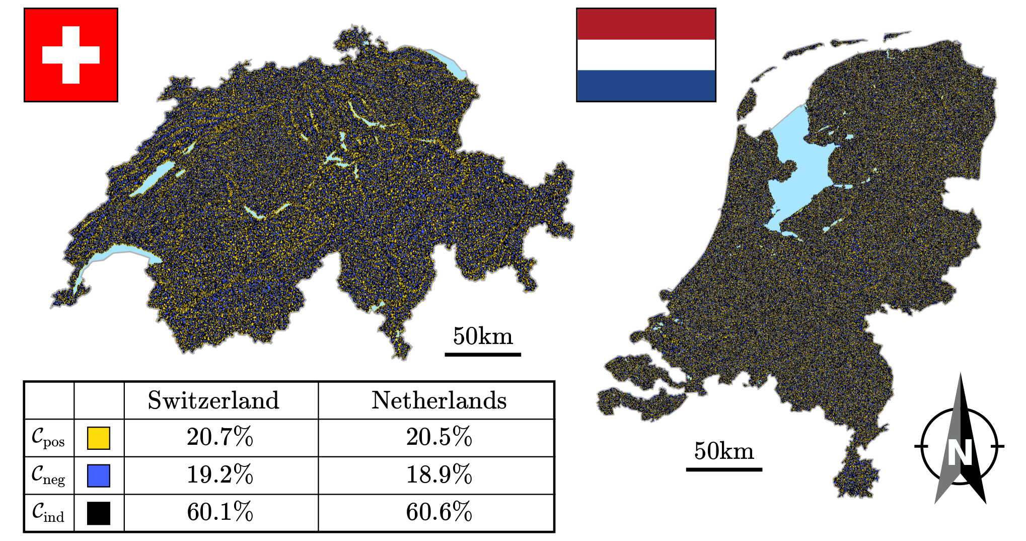
Besides this relation to strong pinning, one might think of completely different applications of Hessian maps and characters, a quite obvious one that comes to mind are natural (topographic) landscapes. Indeed, analyzing the elevation map of different topographic landscapes—we chose Switzerland and the Netherlands as examples, see Fig. 9—one finds in both cases the characters $\mathcal{C}_{\mathrm{pos}}\!\approx\!21\,\%$, $\mathcal{C}_{\mathrm{neg}}\!\approx\!19\,\%$ and $\mathcal{C}_{\mathrm{ind}}\!\approx\!60\,\%$, close to the value for the Gaussian random landscape. This raises interesting questions about universality and the (non-)Gaussianity of natural landscapes.

References

- Tonomura et al. (2001) A. Tonomura, H. Kasai, O. Kamimura, T. Matsuda, K. Harada, Y. Nakayama, J. Shimoyama, K. Kishio, T. Hanaguri, K. Kitazawa, M. Sasase, and S. Okayasu, Observation of individual vortices trapped along columnar defects in high-temperature superconductors, Nature 412, 620 (2001).
- Bending (1999) S. J. Bending, Local magnetic probes of superconductors, Advances in Physics 48, 449 (1999).
- Kirtley (2010) J. R. Kirtley, Fundamental studies of superconductors using scanning magnetic imaging, Reports on Progress in Physics 73, 126501 (2010).
- Suderow et al. (2014) H. Suderow, I. Guillamón, J. G. Rodrigo, and S. Vieira, Imaging superconducting vortex cores and lattices with a scanning tunneling microscope, Superconductor Science and Technology 27, 063001 (2014).
- Thiel et al. (2016) L. Thiel, D. Rohner, M. Ganzhorn, P. Appel, E. Neu, B. Müller, R. Kleiner, D. Koelle, and P. Maletinsky, Quantitative nanoscale vortex imaging using a cryogenic quantum magnetometer, Nature Nanotechnology 11, 677 (2016).
- Straver et al. (2008) E. W. J. Straver, J. E. Hoffman, O. M. Auslaender, D. Rugar, and K. A. Moler, Controlled manipulation of individual vortices in a superconductor, Applied Physics Letters 93, 172514 (2008).
- Auslaender et al. (2009) O. M. Auslaender, L. Luan, E. W. J. Straver, J. E. Hoffman, N. C. Koshnick, E. Zeldov, D. A. Bonn, R. Liang, W. N. Hardy, and K. A. Moler, Mechanics of individual isolated vortices in a cuprate superconductor, Nature Physics 5, 35 (2009).
- Kremen et al. (2016) A. Kremen, S. Wissberg, N. Haham, E. Persky, Y. Frenkel, and B. Kalisky, Mechanical Control of Individual Superconducting Vortices, Nano Letters 16, 1626 (2016).
- Embon et al. (2015) L. Embon, Y. Anahory, A. Suhov, D. Halbertal, J. Cuppens, A. Yakovenko, A. Uri, Y. Myasoedov, M. L. Rappaport, M. E. Huber, A. Gurevich, and E. Zeldov, Probing dynamics and pinning of single vortices in superconductors at nanometer scales, Scientific Reports 5, 7598 (2015).
- Embon et al. (2017) L. Embon, Y. Anahory, Ž. L. Jelić, E. O. Lachman, Y. Myasoedov, M. E. Huber, G. P. Mikitik, A. V. Silhanek, M. V. Milošević, A. Gurevich, and E. Zeldov, Imaging of super-fast dynamics and flow instabilities of superconducting vortices, Nature Communications 8, 85 (2017).
- Kwok et al. (2016) W.-K. Kwok, U. Welp, A. Glatz, A. E. Koshelev, K. J. Kihlstrom, and G. W. Crabtree, Vortices in high-performance high-temperature superconductors, Reports on Progress in Physics 79, 116501 (2016).
- Sadovskyy et al. (2016) I. A. Sadovskyy, Y. Jia, M. Leroux, J. Kwon, H. Hu, L. Fang, C. Chaparro, S. Zhu, U. Welp, J.-M. Zuo, Y. Zhang, R. Nakasaki, V. Selvamanickam, G. W. Crabtree, A. E. Koshelev, A. Glatz, and W.-K. Kwok, Toward Superconducting Critical Current by Design, Advanced Materials 28, 4593 (2016).
- Reichhardt et al. (1995) C. Reichhardt, C. J. Olson, J. Groth, S. Field, and F. Nori, Microscopic derivation of magnetic-flux-density profiles, magnetization hysteresis loops, and critical currents in strongly pinned superconductors, Physical Review B 52, 10441 (1995).
- Olson Reichhardt et al. (2017) C. J. Olson Reichhardt, Y. L. Wang, Z. L. Xiao, W.-K. Kwok, D. Ray, C. Reichhardt, and B. Jankó, Pinning, flux diodes and ratchets for vortices interacting with conformal pinning arrays, Physica C 533, 148 (2017).
- Halpin-Healy and Zhang (1995) T. Halpin-Healy and Y.-C. Zhang, Kinetic roughening phenomena, stochastic growth, directed polymers and all that. Aspects of multidisciplinary statistical mechanics, Physics Reports 254, 215 (1995).
- Blatter et al. (1994) G. Blatter, M. V. Feigel’man, V. B. Geshkenbein, A. I. Larkin, and V. M. Vinokur, Vortices in high-temperature superconductors, Review of Modern Physics 66, 1125 (1994).
- Giamarchi and Le Doussal (1995) T. Giamarchi and P. Le Doussal, Elastic theory of flux lattices in the presence of weak disorder, Phys. Rev. B 52, 1242 (1995).
- Nattermann and Scheidl (2000) T. Nattermann and S. Scheidl, Vortex-glass phases in type-II superconductors, Advances in Physics 49, 607 (2000).
- Bray and Dean (2007) A. J. Bray and D. S. Dean, Statistics of Critical Points of Gaussian Fields on Large-Dimensional Spaces, Physical Review Letters 98, 150201 (2007).
- Fyodorov and Doussal (2018) Y. V. Fyodorov and P. L. Doussal, Hessian spectrum at the global minimum of high-dimensional random landscapes, Journal of Physics A: Mathematical and Theoretical 51, 474002 (2018).
- Freund (1995) I. Freund, Saddles, singularities, and extrema in random phase fields, Physical Review E 52, 2348 (1995).
- Weinrib and Halperin (1982) A. Weinrib and B. I. Halperin, Distribution of maxima, minima, and saddle points of the intensity of laser speckle patterns, Physical Review B 26, 1362 (1982).
- Annibale et al. (2003) A. Annibale, A. Cavagna, I. Giardina, and G. Parisi, Supersymmetric complexity in the Sherrington-Kirkpatrick model, Phys. Rev. E 68, 061103 (2003).
- Bardeen and Stephen (1965) J. Bardeen and M. J. Stephen, Theory of the motion of vortices in superconductors, Physical Review 140, A1197 (1965).
- Yamada and Vilenkin (2018) M. Yamada and A. Vilenkin, Hessian eigenvalue distribution in a random Gaussian landscape, Journal of High Energy Physics 2018, 29 (2018).
- Zinn-Justin (2005) J. Zinn-Justin, Path Integrals in Quantum Mechanics (Oxford University Press, 2005).
- Altland and Simons (2010) A. Altland and B. D. Simons, Condensed Matter Field Theory, 2nd ed. (Cambridge University Press, 2010).
- Craig (1991) J. Craig, A new, simple and exact result for calculating the probability of error for two-dimensional signal constellations, in MILCOM 91 - Conference record, Vol. 2 (1991) p. 571.
- Buchacek et al. (2020) M. Buchacek, V. Geshkenbein, and G. Blatter, Role of rare events in the pinning problem, Phys. Rev. Research 2, 043266 (2020).
- Tanguya and Vettorel (2004) A. Tanguya and T. Vettorel, From weak to strong pinning: A finite size study, Eur. Phys. J. B 38, 71 (2004).
- Cao et al. (2018) X. Cao, S. Bouzat, A. B. Kolton, and A. Rosso, Localization of soft modes at the depinning transition, Phys. Rev. E 97, 022118 (2018).
- Labusch (1969) R. Labusch, Calculation of the critical field gradient in type-II superconductors, Crystal Lattice Defects 1, 1 (1969).
- Montgomery (1958) H. Montgomery, The thermal conductivity of lead at low temperatures, in Proceedings of the Royal Society of London, Series A, Mathematical and Physical Sciences, Vol. 244 (1958) p. 85.
- Kramers (1940) H. A. Kramers, Brownian motion in a field of force and the diffusion model of chemical reactions, Physica 7, 284 (1940).
- Hänggi et al. (1990) P. Hänggi, P. Talkner, and M. Borkovec, Reaction-rate theory: fifty years after Kramers, Review of Modern Physics 62, 251 (1990).