Optimisation of the event-based TOF filtered back-projection for online imaging in total-body J-PET

Multivariate KDE [65] can be applied to the set of most likely points $\{\textbf{{x}}_{\text{MLP}}^{(k)}\}$ of $n$ PET emissions ($k=1\ldots n$), estimated for each LOR from its endpoints (scattering hits in J-PET) and TOF difference $\Delta t$ [83]. The data is processed as density distributions, avoiding the problem of choosing the anchor points, relevant to histo-imaging [71]. It is also justified by the fact that the unknown detector response function, which depends on $\textbf{{x}}_{\text{MLP}}^{(k)}$ and the geometrical orientation of the corresponding LOR, can be perceived as random [76].

Kernel density estimator is defined for a 3D dataset $\{\textbf{{x}}_{\text{MLP}}^{(k)}\}$ as

According to Refs. [12, 11, 7], the definition of $\mathcal{K}(\textbf{{x}})$ is not critical for a large $n$, but the choice of $\mathbf{H}$ is crucial. The algorithms dedicated to find an optimal bandwidth matrix are generally based on the minimisation of the mean squared error (MSE) between $\hat{f}_{n\mathbf{H}}(\textbf{{x}})$ and a tractable approximation that replaces the true density $f_{n}(\textbf{{x}})$. For instance, for a so-called plug-in (PI) estimate, a following function is to be minimised:

Here, an estimator $\hat{\mathbf{\Psi}}_{4}(\mathbf{G})$ substitutes an unknown matrix $\mathbf{\Psi}_{4}$, composed of integrals with the products of the derivatives of $f_{n}(\textbf{{x}})$ (see Ref. [12] for the definition). The elements of $\hat{\mathbf{\Psi}}_{4}(\mathbf{G})$ are calculated from the "measured" $\textbf{{x}}_{\text{MLP}}^{(i)}$ and a pilot bandwidth matrix, set initially as e.g. $\mathbf{G}=g^{2}\mathbf{I}$, where $g>0$, $\mathbf{I}$ – identity matrix [87].

A half-vectorisation operator in (3) is defined as follows:

We utilise the popular R package ’ks’ [11], with two PI estimators for $\hat{\mathbf{H}}_{\text{PI}}$: samse, based on a sum of asymptotic MSE between the elements of $\hat{\mathbf{\Psi}}_{4}(\mathbf{G})$ and $\mathbf{\Psi}_{4}$ [12], and dscalar – a more advanced multistage PI bandwidth selector [7].

According to Eq. (2), all measured data in a form of $\textbf{{x}}_{\text{MLP}}^{(i)}$ is required to estimate the intensity of each voxel x. However, KDE MLP as a reconstruction method could operate in event-by-event mode by changing the order of summation in Eq. (2) or partitioning the data into time frames. $\hat{\mathbf{H}}_{\text{PI}}$ can be predefined or regularly recalculated according to the updated $\hat{\mathbf{\Psi}}_{4}(\mathbf{G})$ by the newly measured data.

FBP is one of the first reconstruction methods introduced for PET [20], which became a standard required by the National Electrical Manufacturers Association (NEMA) for estimating the spatial resolution [53]. In previous works [70, 29], we utilised a 3D FBP with re-projection (FBP 3DRP) from the freeware STIR package [80, 81]. It does not support TOF, multi-layer geometry and the continuous J-PET detectors, and will be used as a reference method in this paper.

We modify FBP as proposed in Ref. [10] – by adding TOF as temporal kernel $h(t)$ that splits 4-dimensional projection functions $p(s,\phi,\zeta,\theta)$ into TOF bins. For the $i$-th bin $h_{i}(t)\equiv h(t-t_{i})$, the filtered function $p^{F}_{i}\equiv p^{F}_{i}(s,\phi,\zeta,\theta,t)$ reads:

We shall treat each emission independently – in list-mode, instead of accumulating them in bins. The summation is made over LORs $(i=1\ldots N_{\text{LOR}})$, while the time difference $t_{i}\equiv\Delta t_{i}=t^{(i)}_{2}-t^{(i)}_{1}$ is related to the $i$-th emitted pair of back-to-back $\gamma$-photons. $p_{i}(s,\phi,\zeta,\theta)$ then becomes a delta-like function (unnormalised unit impulse), and filtering over $s$ will return the filter itself: $p_{i}(s)\ast w(s)=w(s)$, where $w(s)=\mathcal{F}^{-1}W(\omega_{s})$ [69]. The eventually reconstructed image $\hat{f}_{N_{\text{LOR}}}(\textbf{{x}})$ is a sum over the $N_{\text{LOR}}$ back-projections each comprising a single LOR:

Each $p^{F}_{i}$ can be redefined in the $\mathbb{R}^{2}$ space of variables $s$ and $t$, only, as the rest remain constant. For conventional PET scanners, this allows to represent $\mathcal{B}\{p^{F}_{i}\}$ in the image domain as a 3D kernel constituted by the following components:

1. 1)

   TOF function $h(t)$, applied along LOR. For convenience, we redefine it as $h_{\text{TOF}}(l)$, for the distance $l$ from MLP.

2. 2)

   FBP filter $w(s)$, aligned perpendicularly to the transverse projection of the LOR.

The unique J-PET design requires an additional function:

1. 3)

   $h_{Z}(z)$, which represents the axial uncertainty of the two hit positions (Compton scatterings) along scintillator strips.

Despite both $h_{\text{TOF}}(l)$ and $h_{Z}(z)$ are defined by the detection times, they are uncorrelated [55].

The exemplary representation of a three-component kernel applied over the MLP of an emission point is given in Fig. 1. Projection coordinates and detection times are indicated in the inset on top. Since at some distance from MLP the intensity is effectively zero, it is calculated only inside a small ellipsoid – region-of-response (ROR), which volume depends on the time resolution and the properties of the filters.

The standard FBP, for a given view $\phi_{i}$, back-projects $p^{F}_{i}$ to the entire (transverse) image plane. To preserve the proper integration over LORs with an additional $h_{\text{TOF}}(l)$ profile, one should apply weighting normalisation that depends on temporal resolution – CRT. A TOF model for $w(s)$ function was proposed in Ref. [92] as a solution to the following problem:

Selected examples are shown in Fig. 2, a-b. The impact of $\tau$ is easier to track in Fourier space. Relatively large $\tau>10.0$ (in cycles^-1) represent poor timing, as $W(\omega_{s})$ approaches $2\pi\tau|\omega_{s}|$, behaving as pure ramp (Ram-Lak) filter. Conversely, if $\tau$ is very small, $W(\omega_{s})$ becomes a constant $1$ (no filter is required).

The penalisation for the missing data and noise is made by a smoothing window $M(\omega_{s})$ [81]:

Unrelated to FBP kernel components $h_{\text{TOF}}(l)$ and $h_{Z}(z)$ (Fig. 1) mostly affect the axial direction. We shall utilise two different approaches for their definition:

a) Low-pass filtering, introduced in our work [69], aimed at suppressing noise by using Gaussian cumulative distribution function (CDF) – $\cdf(x,\mu,\sigma)$. Kernel components can then be expressed as follows:

b) High-pass filtering is focused on the compensation of the smeared hit positions along $Z$ and the MLP along LOR – a crucial problem for J-PET due to its design. It can be done for an arbitrary profile $h(x)$ by finding its inverse form $h^{-1}(x)$ using the Fourier representation $H(\nu_{x})=\mathcal{F}h(x)$ as follows:

Fig. 2, c-d depicts Gaussian $h(x)$ and $H(\nu_{x})$ with SD $\sigma_{x}$, as well as their inverse forms $h^{-1}(x)$ and $H^{-1}(\nu_{x})$. An example of the apodised $H^{-1}_{\text{cut}}(\nu_{x})$ by the cut-off $\pm\nu_{\text{cut}}$ ($\nu_{\text{Nq}}$ denotes Nyquist frequency) is shown as dashed lines.

Contrary to the low-pass filtering, the inverse functions $h^{-1}_{\text{TOF}}(l)$ and $h^{-1}_{Z}(z)$ must be rigorously calculated from CDF profiles with SDs that reflect the intrinsic resolution of the scanner:

High-pass filtering increases the minimal size of the allocated ROR volume. The dashed lines in Fig. 2, c denote the $\pm 3.5\sigma$ truncation range, suitable for a Gaussian CDF (red curve) – see Refs. [13, 76]. For the inverse $h^{-1}(x)$, however, it ought to be enlarged significantly.

For convenience, we shall use both "event-based TOF FBP" and "TOF FBP" notation in this paper. The script for the algorithm is written in R using vectorised functions [59]. The latest version allows multi-threading, but most of the tests were run in a single-thread mode on a regular node of CIŚ cluster²² 2 CIŚ – Centrum Informatyczne Świerk: https://www.cis.gov.pl/ (Intel Xeon E5-2680v2, 128 GB RAM).

We ran simulations for the selected NEMA sources, phantoms, scanners and interactions of the 511-keV photons with the detectors using the Geant4 Application for Tomographic Emission (GATE) framework [22, 21]. In order to focus exclusively on the reconstruction methods, an ideal configuration was chosen: a single cylindrical layer of plastic BC-420 scintillator strips placed side-by-side. The datasets simulated for our work [29] were used to study the spatial resolution and validate the earlier results, for a scanner of the radius $R=425.6$ mm, composed of 382 strips with the size 7 mm $\times$ 20 mm $\times$ 500 mm. A very similar geometry was defined for the other phantoms, to be consistent with Refs. [27, 62]: 384 strips, each of 7 mm $\times$ 19 mm $\times$ 500 mm size, $R=427.8$ mm. The axial length of $50$ cm is a good middle-point that minimises the parallax effect (see Ref. [27]), yet allows generalisation over tomographs with large AFOV.

Post-simulation smearing of hit positions and times of hits was performed to represent signal readouts with CRT in the $50-500$-ps range. The highest value is close to the results from the early experiments with 3-layer "big barrel" J-PET prototype [55, 58, 69], the lowest – reflects a theoretical minimum for BC-420 scintillators with WLS attached, previsioned for the future development of J-PET [47]. We shall refer to the latter as "Ideal + WLS". Selected datasets were post-smeared to simulate non-collinearity [40], with a rough approximation of positron transport for a number of radionuclides [44], using a two-exponential model (see e.g. Ref. [30]). The details are given in A.

For the spatial resolution analysis, a point-like $1$-mm spherical source was defined in GATE inside a $382$-strip ideal J-PET, with an activity of $370$ kBq [29]. A separate simulation was run for the object put at six NEMA locations, varying its transverse ($y=10$ mm, $100$ mm and $200$ mm) and axial position ($z=0$ mm and $187.5$ mm), with fixed $x=0$ mm (Fig. 3, a). A total of $150,000$ events were acquired per run.

The next simulated object was the NEMA-defined IEC phantom, used for the analysis of the image quality [53]. It was aligned axially as shown in Fig. 3, b-c, with the interior length $220$ mm. Hot lesions, represented by the spheres (with capillaries) of diameters $10$ mm, $13$ mm, $17$ mm and $22$ mm, were filled with radioactive water, which activity was set four times higher than in the background volume. No lung insert was simulated along the central axis, replaced by a cold cylinder. The total injected activity amounted to $53$ MBq for $\hphantom{{}^{\text{18}}_{\text{}}}{\vphantom{\text{X}}}{}^{\mathchoice{\hbox to0.0pt{\hss$\displaystyle\vphantom{\smash[t]{\text{2}}}\text{18}$}}{\hbox to0.0pt{\hss$\textstyle\vphantom{\smash[t]{\text{2}}}\text{18}$}}{\hbox to0.0pt{\hss$\scriptstyle\vphantom{\smash[t]{\text{2}}}\text{18}$}}{\hbox to0.0pt{\hss$\scriptscriptstyle\vphantom{\smash[t]{\text{2}}}\text{18}$}}}\kern 0.0pt\text{F}\text{\hskip 1.29167pt--\hskip 1.29167pt}\text{FDG}$ dissolved in water. Two datasets were used for the analysis, comprising $\sim 40$ mln and $\sim 80$ mln coincidences recorded in a $384$-strip $50$-cm long J-PET scanner. It reflects the times of scan of $\sim 10$ min or $\sim 20$ min, respectively.

Finally, in order to test and evaluate the TOF FBP method for the setup most resembling diagnostic practices, we simulated one bed position of the eXtended CArdiac-Torso (XCAT) static phantom, using the software, developed by [66, 67]. Separate voxelised images for the activity and attenuation factors were generated from a female template. The phantom was aligned as shown in Fig. 3, d: the centre of its volume was shifted $-385$ mm along $Z$ from the J-PET central point. The activity concentration was adjusted to match the weight-based $5.3$ MBq/kg level of the simulated NEMA IEC, having reached $350$ MBq for a $66$-kg body mass. We kept the default ratios set for various tissues in the configuration files, which resemble an early distribution of positron emissions during the first $10-20$ min after intravenous administration of $\hphantom{{}^{\text{18}}_{\text{}}}{\vphantom{\text{X}}}{}^{\mathchoice{\hbox to0.0pt{\hss$\displaystyle\vphantom{\smash[t]{\text{2}}}\text{18}$}}{\hbox to0.0pt{\hss$\textstyle\vphantom{\smash[t]{\text{2}}}\text{18}$}}{\hbox to0.0pt{\hss$\scriptstyle\vphantom{\smash[t]{\text{2}}}\text{18}$}}{\hbox to0.0pt{\hss$\scriptscriptstyle\vphantom{\smash[t]{\text{2}}}\text{18}$}}}\kern 0.0pt\text{F}$-type radionuclide [79]. An additional $12$-mm hot spherical lesion was simulated in the right lung at $(x,y,z)=(-50$ mm, $60$ mm, $60$ mm), four times more active than the neighbouring tissue. The simulated $10$-minute scan produced $119.5$ mln coincidences in total.

To compensate for boundary axial effects in the scanners, sensitivity maps were simulated using a hybrid MC/analytical approach from Ref. [76]. An alternative correction method of re-projection [26] is incorporated in FBP 3DRP, but it is slow and more beneficial for short AFOV. No restriction for maximal obliqueness $\theta$ was imposed.

The data were pre-selected by a $3$-ns time window, to obtain coincident interactions of photons with the detector (refer to Ref. [29] for the discussion on selection criteria). Only true events were taken into account, without scatter and random correction (there are multiple ongoing studies dedicated to the latter, e.g. Ref. [68]). The resulting numbers of true coincidences were $\sim 10$ mln and $\sim 20$ mln for the two datasets of IEC simulation, and $16.5$ mln – for XCAT.

Attenuation correction for IEC and XCAT was applied on the fly, as a recalculation of a radiological path for each emission by a modified Siddon algorithm [33], using the predefined attenuation factors (shown in Fig. 3 in different colours). This method could not be applied to KDE MLP, so we employed a simplified solution for IEC (only): true events were resampled according to the statistics for the genuine annihilation points, assigned by GATE. Only the data from the lower half of the phantom ($z\leq 0$ mm) were considered, avoiding the regions with spheres. To equalise the attenuated activity levels in the background volume, about one-third of the coincidences had to be dropped, hence a larger subset from the initial $80$-mln statistics was taken to obtain the required 10-mln true events.

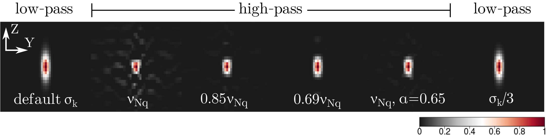
Fig. 4 shows the axial cross-sections of a $1$-mm spherical source in a 382-strip scanner with SiPM readout, reconstructed using various definitions of TOF- and $Z$-components of the kernel. Voxel size was defined by a virtual $96$-ring, $N$-strip scanner of the radius $R$: $\Delta x=\Delta y=\Delta s/2\approx 1.8$ mm and $\Delta z\approx 2.6$ mm [29], where $\Delta s=\pi R/N$ [4]. The source was located at ($x_{\text{src}}$, $y_{\text{src}}$, $z_{\text{src}}$) = ($0$ mm, $100$ mm, $0$ mm). TOF FBP regularisation (9) was not applied as it is redundant for a tiny $1$-mm object.

High-pass filters $h^{-1}_{\text{TOF}}(l)$ and $h^{-1}_{Z}(z)$ produce higher axial resolution than the initial low-pass Gaussians (12), but also enhance background noise. It could be eliminated by the adjustment of smoothing and apodisation parameters $\alpha$ and $\nu_{\text{cut}}$ (see Fig. 2, d). The cut-off $\nu_{\text{cut}}$ in Fig. 4 is represented as a fraction of a Nyquist frequency $\nu_{\text{Nq}}=1/(2\sigma_{k})$. An additional low-pass case is shown on the right: $\sigma_{\text{TOF}}$ and $\sigma_{Z}$ are decreased three times from the "initial" values, estimated from CRT and $\Delta z$, respectively. That implies $\sigma_{\text{TOF}}\approx 5.0$ mm and $\sigma_{Z}\approx 0.4$ mm for $\text{CRT}=235$ ps and $\Delta z=2.6$ mm.

Estimated PSF values for the selected kernel definitions are presented in Table 1. As a reference point, the results obtained by KDE MLP and FBP 3DRP [29] are added. The event-based TOF FBP produces slightly better $\text{PSF}_{X,Y}$, but worse axial resolution for the Gaussian-defined kernel components. The best $\text{PSF}_{Z}$ is obtained for the ideal ramp and high-pass filters $h^{-1}_{\text{TOF}}(l)$ and $h^{-1}_{Z}(z)$, without cut-offs or smoothing, i.e. $\alpha=1$, $\nu_{\text{cut}}=\nu_{\text{Nq}}$. However, the imposed noise and distortion are too high (Fig. 4).

As a reasonable trade-off, we have fixed the cut-off at $\nu_{\text{cut}}=0.85\,\nu_{\text{Nq}}$ and conducted a detailed study for the source at six NEMA-defined locations (see Fig. 3, a). The estimated PSF values are shown in Fig. 5 for three readouts, as in Ref. [29]: PM tubes (PMT, $\text{CRT}=315$ ps), SiPM ($\text{CRT}=235$ ps) and ideal case with WLS ($\text{CRT}=50$ ps). TOF FBP and FBP 3DRP produce similar results on the transverse plane, outperforming KDE MLP (no FBP filter) even for the best timing. As for axial resolution, high-pass filtering decreases $\text{PSF}_{Z}$ by about $\times 1.5$ times, compared to FBP 3DRP or KDE MLP. More details are revealed in A.

As the main object of study, we chose a relatively small $10$-mln statistics of true coincidences (roughly a $10$-min scan), registered from the NEMA IEC phantom in a $384$-strip J-PET scanner. The cut-off $\nu_{\text{cut}}=0.85\,\nu_{\text{Nq}}$ used in the previous section is presumably too high, representing the axial resolution achievable for long scans. We thus changed $\nu_{\text{cut}}$ in a $0.6-0.9\,\nu_{\text{Nq}}$ range, considered a larger $20$ mln dataset, as well as the reduced smoothing $\alpha<1$. The $235$-ps readout (SiPM) was chosen, relevant to current J-PET prototypes. Unlike previously, a symmetric voxel $\Delta x=\Delta y=\Delta z=1.8$ mm was used, to avoid distortion caused by post-filtering, and a modified FBP from Eq. (9). The regularisation $\tau$ was adjusted, with fixed $\omega_{c}=\omega_{\text{Nq}}$ and $\alpha=1$.

The results for $\tau=7.5$, explored to be close to the optimal, are presented in Fig. 6. The images on the left show the outcomes after MPF has been applied, using a spherical mask of $4$-voxel radius. High-pass filtering produces less random and even quasi-regular intensity levels on the background, compared to the case of low-pass $h_{\text{TOF}}(l)$ and $h_{Z}(z)$ (denoted as "default").

The histograms of the errors $\text{Err}(\textbf{{x}}_{i})$ from Eq. (20), shown on top, generally reflect a combination of Gaussian profiles. However, the distributions are more asymmetric than in the "default" case, mainly caused by the negative lobes – voxels with intensities below zero. Such offset remains even after post-filtering and for a hybrid 3D kernel – a low-pass $h_{\text{TOF}}(l)$, combined with $h_{Z}^{-1}(z)$ (shown for $\nu_{\text{cut}}=0.85\nu_{\text{Nq}}$). Improvement can also be achieved by imposing a smoothing window, as depicted for $\alpha=0.575$ and 20-mln dataset, but that would worsen axial resolution to the low-pass levels ($\text{PSF}_{Z}>15$ mm), which we observed in axial intensity profiles (not shown).

Table 2 reveals the estimated image quality parameters of NEMA IEC for three spheres and three reconstructions (all with MPF). The first two correspond to $h^{-1}_{\text{TOF}}(l)$ and $h^{-1}_{Z}(z)$ ($\nu_{\text{cut}}=0.6\,\nu_{\text{Nq}}$) for $10$-mln and $20$-mln subsets of true events, the third – to the Gaussian CDFs and $10$-mln statistics. High-pass filtering produces higher CRCs, calculated for the hot $13$-mm and $22$-mm spheres, but not for the cold $28$-mm one. BVs are generally better for the reference (low-pass) image, indicating the lesser amount of distortion and noise. Image quality is susceptible to MPF mask, too: CRC for $13$-mm and $22$-mm spheres are lower for the $20$-mln set than for the $10$-mln one.

For the reference TOF FBP reconstruction, made using low-pass filters and MPF, the estimated ${\text{MSE}=3.0\cdot 10^{-3}}$ on a normalised $\left[0,1\right]$ intensity scale was lower than for the images, obtained from $10$-mln statistics using $h^{-1}_{\text{TOF}}(l)$ and $h^{-1}_{Z}(z)$ (e.g. $\text{MSE}=\,4.0\cdot 10^{-3}$ for $\nu_{\text{cut}}=0.6\,\nu_{\text{Nq}}$ shown in Fig. 6 on the top right). Lower $\text{MSE}=2.5\cdot 10^{-3}$ was achieved only for a $20$-mln dataset with a substantial smoothing $\alpha=0.575$.

Worse MSE, spatial resolution, deteriorated by the apodisation and the smoothing, noise issues with asymmetric $\text{Err}(\textbf{{x}}_{i})$ distributions and image quality, rather not superior to the alternative kernel definition, do not favour the usage of high-pass filtering for online scans. Moreover, the inverse Gaussians $h^{-1}_{\text{TOF}}(l)$ and $h^{-1}_{Z}(z)$ require a larger ROR span (see Fig. 2, c), which slows the computing performance. On the other hand, such filters would be beneficial for tomographs of higher sensitivity and longer diagnostic times. We shall focus on a low-pass representation of $h_{\text{TOF}}(l)$ and $h_{Z}(z)$ in the further analysis.

References

- Allemand et al. [1980] Allemand, R., Gresset, C., Vacher, J.. Potential advantages of a cesium fluoride scintillator for a time-of-flight positron camera. J Nucl Med 1980;21(2):153–155. URL: http://www.ncbi.nlm.nih.gov/pubmed/6965404.
- Ariño-Estrada et al. [2019] Ariño-Estrada, G., Mitchell, G.S., Kim, H., Du, J., Kwon, S.I., Cirignano, L.J., Shah, K.S., Cherry, S.R.. First Cerenkov charge-induction (CCI) TlBr detector for TOF-PET and proton range verification. Physics in Medicine & Biology 2019;64(17):175001. URL: https://iopscience.iop.org/article/10.1088/1361-6560/ab35c4. doi:10.1088/1361-6560/ab35c4.
- Badawi et al. [2019] Badawi, R.D., Shi, H., Hu, P., Chen, S., Xu, T., Price, P.M., Ding, Y., Spencer, B.A., Nardo, L., Liu, W., Bao, J., Jones, T., Li, H., Cherry, S.R.. First Human Imaging Studies with the EXPLORER Total-Body PET Scanner. J Nucl Med 2019;60(3):299–303. URL: http://jnm.snmjournals.org/lookup/doi/10.2967/jnumed.119.226498. doi:10.2967/jnumed.119.226498.
- Bailey et al. [2005] Bailey, D.L., Townsend, D.W., Valk, P.E., Maisey, M.N., editors. Positron Emission Tomography. London: Springer-Verlag, 2005. URL: http://link.springer.com/10.1007/b136169. doi:10.1007/b136169.
- Budinger [1983] Budinger, T.F.. Time-of-flight positron emission tomography: status relative to conventional PET. J Nucl Med 1983;24(1):73–78. URL: http://www.ncbi.nlm.nih.gov/pubmed/6336778.
- Carter et al. [2020] Carter, L.M., Kesner, A.L., Pratt, E.C., Sanders, V.A., Massicano, A.V.F., Cutler, C.S., Lapi, S.E., Lewis, J.S.. The Impact of Positron Range on PET Resolution, Evaluated with Phantoms and PHITS Monte Carlo Simulations for Conventional and Non-conventional Radionuclides. Molecular Imaging and Biology 2020;22(1):73–84. URL: http://link.springer.com/10.1007/s11307-019-01337-2. doi:10.1007/s11307-019-01337-2.
- Chacón and Duong [2010] Chacón, J.E., Duong, T.. Multivariate plug-in bandwidth selection with unconstrained pilot bandwidth matrices. TEST 2010;19(2):375–398. URL: http://link.springer.com/10.1007/s11749-009-0168-4. doi:10.1007/s11749-009-0168-4.
- Cloquet and Defrise [2011] Cloquet, C., Defrise, M.. Does OSEM achieve the lowest variance? In: 2011 IEEE Nucl. Sci. Symp. Conf. Rec. IEEE; 2011. p. 2360–2365. URL: http://ieeexplore.ieee.org/document/6153880/. doi:10.1109/NSSMIC.2011.6153880.
- Conti [2011] Conti, M.. Focus on time-of-flight PET: the benefits of improved time resolution. EJNMMI 2011;38(6):1147–1157. URL: http://www.ncbi.nlm.nih.gov/pubmed/21229244. doi:10.1007/s00259-010-1711-y.
- Conti et al. [2005] Conti, M., Bendriem, B., Casey, M., Chen, M., Kehren, F., Michel, C., Panin, V.. First experimental results of time-of-flight reconstruction on an LSO PET scanner. Phys Med Biol 2005;50(19):4507–4526. URL: https://iopscience.iop.org/article/10.1088/0031-9155/50/19/006. doi:10.1088/0031-9155/50/19/006.
- Duong [2007] Duong, T.. ks: Kernel Density Estimation and Kernel Discriminant Analysis for Multivariate Data in R. J Stat Softw 2007;21(7):1–16. URL: http://www.jstatsoft.org/v21/i07/. doi:10.18637/jss.v021.i07.
- Duong and Hazelton [2003] Duong, T., Hazelton, M.. Plug-in bandwidth matrices for bivariate kernel density estimation. J Nonparametr Stat 2003;15(1):17–30. URL: http://www.tandfonline.com/doi/abs/10.1080/10485250306039. doi:10.1080/10485250306039.
- Efthimiou et al. [2019] Efthimiou, N., Emond, E., Wadhwa, P., Cawthorne, C., Tsoumpas, C., Thielemans, K.. Implementation and validation of time-of-flight PET image reconstruction module for listmode and sinogram projection data in the STIR library. Phys Med Biol 2019;64(3):035004. URL: https://iopscience.iop.org/article/10.1088/1361-6560/aaf9b9. doi:10.1088/1361-6560/aaf9b9.
- Fabijańska and Sankowski [2011] Fabijańska, A., Sankowski, D.. Noise adaptive switching median-based filter for impulse noise removal from extremely corrupted images. IET Image Proc 2011;5(5):472–480. URL: https://digital-library.theiet.org/content/journals/10.1049/iet-ipr.2009.0178. doi:10.1049/iet-ipr.2009.0178.
- Ferrara and Mansi [2011] Ferrara, R., Mansi, L.. Paul Suetens (ed): Fundamentals of Medical Imaging (2nd edition). EJNMMI 2011;38(2):409–409. URL: http://link.springer.com/10.1007/s00259-010-1694-8. doi:10.1007/s00259-010-1694-8.
- Ferrero et al. [2018] Ferrero, V., Fiorina, E., Morrocchi, M., Pennazio, F., Baroni, G., Battistoni, G., Belcari, N., Camarlinghi, N., Ciocca, M., Del Guerra, A., Donetti, M., Giordanengo, S., Giraudo, G., Patera, V., Peroni, C., Rivetti, A., Rolo, M.D.d.R., Rossi, S., Rosso, V., Sportelli, G., Tampellini, S., Valvo, F., Wheadon, R., Cerello, P., Bisogni, M.G.. Online proton therapy monitoring: clinical test of a Silicon-photodetector-based in-beam PET. Sci Rep 2018;8(1):4100. URL: http://www.nature.com/articles/s41598-018-22325-6. doi:10.1038/s41598-018-22325-6.
- Fiorina et al. [2018] Fiorina, E., Ferrero, V., Pennazio, F., Baroni, G., Battistoni, G., Belcari, N., Cerello, P., Camarlinghi, N., Ciocca, M., Del Guerra, A., Donetti, M., Ferrari, A., Giordanengo, S., Giraudo, G., Mairani, A., Morrocchi, M., Peroni, C., Rivetti, A., Da Rocha Rolo, M., Rossi, S., Rosso, V., Sala, P., Sportelli, G., Tampellini, S., Valvo, F., Wheadon, R., Bisogni, M.. Monte Carlo simulation tool for online treatment monitoring in hadrontherapy with in-beam PET: A patient study. Phys Med 2018;51:71–80. URL: https://linkinghub.elsevier.com/retrieve/pii/S1120179718304587. doi:10.1016/j.ejmp.2018.05.002.
- Grant et al. [2016] Grant, A.M., Deller, T.W., Khalighi, M.M., Maramraju, S.H., Delso, G., Levin, C.S.. NEMA NU 2-2012 performance studies for the SiPM-based ToF-PET component of the GE SIGNA PET/MR system. Med Phys 2016;43(5):2334. URL: http://www.ncbi.nlm.nih.gov/pubmed/27147345. doi:10.1118/1.4945416.
- Gundacker et al. [2013] Gundacker, S., Auffray, E., Frisch, B., Jarron, P., Knapitsch, A., Meyer, T., Pizzichemi, M., Lecoq, P.. Time of flight positron emission tomography towards 100ps resolution with L(Y)SO: an experimental and theoretical analysis. JINST 2013;8(07):P07014–P07014. URL: https://iopscience.iop.org/article/10.1088/1748-0221/8/07/P07014. doi:10.1088/1748-0221/8/07/P07014.
- Helgason [1984] Helgason, S.. Groups and geometric analysis: integral geometry, invariant differential operators, and spherical functions. Orlando, FL: Academic Press, 1984.
- Jan et al. [2011] Jan, S., Benoit, D., Becheva, E., Carlier, T., Cassol, F., Descourt, P., Frisson, T., Grevillot, L., Guigues, L., Maigne, L., Morel, C., Perrot, Y., Rehfeld, N., Sarrut, D., Schaart, D.R., Stute, S., Pietrzyk, U., Visvikis, D., Zahra, N., Buvat, I.. GATE V6: a major enhancement of the GATE simulation platform enabling modelling of CT and radiotherapy. Phys Med Biol 2011;56(4):881–901. URL: http://www.ncbi.nlm.nih.gov/pubmed/21248393. doi:10.1088/0031-9155/56/4/001.
- Jan et al. [2004] Jan, S., Santin, G., Strul, D., Staelens, S., Assié, K., Autret, D., Avner, S., Barbier, R., Bardiès, M., Bloomfield, P.M., Brasse, D., Breton, V., Bruyndonckx, P., Buvat, I., Chatziioannou, A.F., Choi, Y., Chung, Y.H., Comtat, C., Donnarieix, D., Ferrer, L., Glick, S.J., Groiselle, C.J., Guez, D., Honore, P.F., Kerhoas-Cavata, S., Kirov, A.S., Kohli, V., Koole, M., Krieguer, M., van der Laan, D.J., Lamare, F., Largeron, G., Lartizien, C., Lazaro, D., Maas, M.C., Maigne, L., Mayet, F., Melot, F., Merheb, C., Pennacchio, E., Perez, J., Pietrzyk, U., Rannou, F.R., Rey, M., Schaart, D.R., Schmidtlein, C.R., Simon, L., Song, T.Y., Vieira, J.M., Visvikis, D., de Walle, R.V., Wieërs, E., Morel, C.. GATE: a simulation toolkit for PET and SPECT. Phys Med Biol 2004;49(19):4543–4561. URL: https://iopscience.iop.org/article/10.1088/0031-9155/49/19/007. doi:10.1088/0031-9155/49/19/007.
- Kadrmas et al. [2009] Kadrmas, D.J., Casey, M.E., Conti, M., Jakoby, B.W., Lois, C., Townsend, D.W.. Impact of time-of-flight on PET tumor detection. J Nucl Med 2009;50(8):1315–1323. URL: http://www.ncbi.nlm.nih.gov/pubmed/19617317. doi:10.2967/jnumed.109.063016.
- Karp et al. [2008] Karp, J.S., Surti, S., Daube-Witherspoon, M.E., Muehllehner, G.. Benefit of Time-of-Flight in PET: Experimental and Clinical Results. J Nucl Med 2008;49(3):462–470. URL: http://jnm.snmjournals.org/cgi/doi/10.2967/jnumed.107.044834. doi:10.2967/jnumed.107.044834.
- Karp et al. [2020] Karp, J.S., Viswanath, V., Geagan, M.J., Muehllehner, G., Pantel, A.R., Parma, M.J., Perkins, A.E., Schmall, J.P., Werner, M.E., Daube-Witherspoon, M.E.. PennPET Explorer: Design and Preliminary Performance of a Whole-Body Imager. J Nucl Med 2020;61(1):136–143. URL: http://jnm.snmjournals.org/lookup/doi/10.2967/jnumed.119.229997. doi:10.2967/jnumed.119.229997.
- Kinahan and Rogers [1989] Kinahan, P.E., Rogers, J.G.. Analytic 3D image reconstruction using all detected events. IEEE Trans Nucl Sci 1989;36(1):964–968. URL: http://ieeexplore.ieee.org/document/34585/. doi:10.1109/23.34585.
- Kopka and Klimaszewski [2020] Kopka, P., Klimaszewski, K.. Reconstruction of the NEMA IEC Body Phantom from J-PET Total-body Scanner Simulation Using STIR. APPB 2020;51(1):357. URL: http://www.actaphys.uj.edu.pl/findarticle?series=Reg&vol=51&page=357. doi:10.5506/APhysPolB.51.357.
- Korcyl et al. [2018] Korcyl, G., Hiesmayr, B.C., Jasinska, B., Kacprzak, K., Kajetanowicz, M., Kisielewska, D., Kowalski, P., Kozik, T., Krawczyk, N., Krzemien, W., Kubicz, E., Bialas, P., Mohammed, M., Niedzwiecki, S., Pawlik-Niedzwiecka, M., Palka, M., Raczynski, L., Rajda, P., Rudy, Z., Salabura, P., Sharma, N.G., Sharma, S., Curceanu, C., Shopa, R.Y., Skurzok, M., Silarski, M., Strzempek, P., Wieczorek, A., Wislicki, W., Zaleski, R., Zgardzinska, B., Zielinski, M., Moskal, P., Czerwinski, E., Dulski, K., Flak, B., Gajos, A., Glowacz, B., Gorgol, M.. Evaluation of Single-Chip, Real-Time Tomographic Data Processing on FPGA SoC Devices. IEEE Trans Med Imagin 2018;37(11):2526–2535. URL: https://ieeexplore.ieee.org/document/8360475/. doi:10.1109/TMI.2018.2837741.
- Kowalski et al. [2018] Kowalski, P., Wiślicki, W., Shopa, R.Y., Raczyński, L., Klimaszewski, K., Curcenau, C., Czerwiński, E., Dulski, K., Gajos, A., Gorgol, M., Gupta-Sharma, N., Hiesmayr, B., Jasińska, B., Kapłon, Ł., Kisielewska-Kamińska, D., Korcyl, G., Kozik, T., Krzemień, W., Kubicz, E., Mohammed, M., Niedźwiecki, S., Pałka, M., Pawlik-Niedźwiecka, M., Raj, J., Rakoczy, K., Rudy, Z., Sharma, S., Shivani, S., Silarski, M., Skurzok, M., Zgardzińska, B., Zieliński, M., Moskal, P.. Estimating the NEMA characteristics of the J-PET tomograph using the GATE package. Phys Med Biol 2018;63(16):165008. URL: https://iopscience.iop.org/article/10.1088/1361-6560/aad29b. doi:10.1088/1361-6560/aad29b.
- Le Loirec and Champion [2007] Le Loirec, C., Champion, C.. Track structure simulation for positron emitters of medical interest. Part I: The case of the allowed decay isotopes. Nuclear Instruments and Methods in Physics Research Section A: Accelerators, Spectrometers, Detectors and Associated Equipment 2007;582(2):644–653. URL: https://linkinghub.elsevier.com/retrieve/pii/S0168900207018578. doi:10.1016/j.nima.2007.08.159.
- Lecoq [2017] Lecoq, P.. Pushing the Limits in Time-of-Flight PET Imaging. IEEE Trans Radiat Plasma Med Sci 2017;1(6):473–485. URL: https://ieeexplore.ieee.org/document/8049484/. doi:10.1109/TRPMS.2017.2756674.
- Lecoq et al. [2020] Lecoq, P., Morel, C., Prior, J.O., Visvikis, D., Gundacker, S., Auffray, E., Križan, P., Turtos, R.M., Thers, D., Charbon, E., Varela, J., de La Taille, C., Rivetti, A., Breton, D., Pratte, J.F., Nuyts, J., Surti, S., Vandenberghe, S., Marsden, P., Parodi, K., Benlloch, J.M., Benoit, M.. Roadmap toward the 10 ps time-of-flight PET challenge. Physics in Medicine & Biology 2020;65(21):21RM01. URL: https://iopscience.iop.org/article/10.1088/1361-6560/ab9500. doi:10.1088/1361-6560/ab9500.
- Li et al. [2016] Li, S., Wang, M., Hou, H., Yang, J., Wang, X.. Fast algorithm for calculating the radiological path in fan-beam CT image reconstruction. Optik 2016;127(5):2973–2977. URL: https://linkinghub.elsevier.com/retrieve/pii/S0030402615019439. doi:10.1016/j.ijleo.2015.12.034.
- López-Montes et al. [2020] López-Montes, A., Galve, P., Udias, J.M., Cal-González, J., Vaquero, J.J., Desco, M., Herraiz, J.L.. Real-Time 3D PET Image with Pseudoinverse Reconstruction. Applied Sciences 2020;10(8):2829. URL: https://www.mdpi.com/2076-3417/10/8/2829. doi:10.3390/app10082829.
- Marafini et al. [2015] Marafini, M., Attili, A., Battistoni, G., Belcari, N., Bisogni, M., Camarlinghi, N., Cappucci, F., Cecchetti, M., Cerello, P., Ciciriello, F., Cirrone, G., Coli, S., Corsi, F., Cuttone, G., De Lucia, E., Ferretti, S., Faccini, R., Fiorina, E., Frallicciardi, P., Giraudo, G., Kostara, E., Kraan, A., Licciulli, F., Liu, B., Marino, N., Marzocca, C., Matarrese, G., Morone, C., Morrocchi, M., Muraro, S., Patera, V., Pennazio, F., Peroni, C., Piersanti, L., Piliero, M., Pirrone, G., Rivetti, A., Romano, F., Rosso, V., Sala, P., Sarti, A., Sciubba, A., Sportelli, G., Voena, C., Wheadon, R., Del Guerra, A.. The INSIDE Project: Innovative Solutions for In-Beam Dosimetry in Hadrontherapy. APPA 2015;127(5):1465–1467. URL: http://przyrbwn.icm.edu.pl/APP/PDF/127/a127z5p06.pdf. doi:10.12693/APhysPolA.127.1465.
- Marcinkowski et al. [2016] Marcinkowski, R., Mollet, P., Van Holen, R., Vandenberghe, S.. Sub-millimetre DOI detector based on monolithic LYSO and digital SiPM for a dedicated small-animal PET system. Phys Med Biol 2016;61(5):2196–2212. URL: https://iopscience.iop.org/article/10.1088/0031-9155/61/5/2196. doi:10.1088/0031-9155/61/5/2196.
- Matej et al. [2016] Matej, S., Daube-Witherspoon, M.E., Karp, J.S.. Analytic TOF PET reconstruction algorithm within DIRECT data partitioning framework. Phys Med Biol 2016;61(9):3365–3386. URL: https://iopscience.iop.org/article/10.1088/0031-9155/61/9/3365. doi:10.1088/0031-9155/61/9/3365.
- Matej et al. [2009] Matej, S., Surti, S., Jayanthi, S., Daube-Witherspoon, M., Lewitt, R., Karp, J.. Efficient 3-D TOF PET Reconstruction Using View-Grouped Histo-Images: DIRECT – Direct Image Reconstruction for TOF. IEEE Trans Med Imaging 2009;28(5):739–751. URL: http://ieeexplore.ieee.org/document/4749317/. doi:10.1109/TMI.2008.2012034.
- Miyata et al. [2006] Miyata, M., Tomita, H., Watanabe, K., Kawarabayashi, J., Iguchi, T.. Development of TOF-PET using Cherenkov Radiation. Journal of Nuclear Science and Technology 2006;43(4):339–343. URL: http://www.tandfonline.com/doi/abs/10.1080/18811248.2006.9711101. doi:10.1080/18811248.2006.9711101.
- Moses [2011] Moses, W.W.. Fundamental limits of spatial resolution in PET. Nuclear Instruments and Methods in Physics Research Section A: Accelerators, Spectrometers, Detectors and Associated Equipment 2011;648:S236–S240. URL: https://linkinghub.elsevier.com/retrieve/pii/S0168900210026276. doi:10.1016/j.nima.2010.11.092.
- Moskal [2018] Moskal, P.. J-PET: Towards total-body modular PET from plastic scintillators. In: Abstracts of the Total Body PET Conference 2018, EJNMMI Physics. volume 5; 2018. p. S2. URL: https://ejnmmiphys.springeropen.com/articles/10.1186/s40658-018-0218-7. doi:10.1186/s40658-018-0218-7.
- Moskal et al. [2020] Moskal, P., Bednarski, T., Niedźwiecki, S., Silarski, M., Czerwiński, E., Kozik, T., Chhokar, J., Bała, M., Curceanu, C., Del Grande, R., Dadgar, M., Dulski, K., Gajos, A., Gorgol, M., Gupta-Sharma, N., Hiesmayr, B.C., Jasińska, B., Kacprzak, K., Kapłon, Ł., Karimi, H., Kisielewska, D., Klimaszewski, K., Korcyl, G., Kowalski, P., Krawczyk, N., Krzemień, W., Kubicz, E., Mohammed, M., Pałka, M., Pawlik-Niedźwiecka, M., Raczyński, L., Raj, J., Sharma, S., Shivani, S., Shopa, R.Y., Skurzok, M., Stȩpień, E., Wiślicki, W., Zgardzińska, B.. Synchronisation and calibration of the 24-modules J-PET prototype with 300 mm axial field of view. IEEE Transactions on Instrumentation and Measurement 2020;:1–1URL: https://ieeexplore.ieee.org/document/9173708/. doi:10.1109/TIM.2020.3018515.
- Moskal et al. [2019a] Moskal, P., Jasińska, B., Stȩpień, E.Ł., Bass, S.D.. Positronium in medicine and biology. Nature Reviews Physics 2019a;1(9):527–529. URL: http://www.nature.com/articles/s42254-019-0078-7. doi:10.1038/s42254-019-0078-7.
- Moskal et al. [2019b] Moskal, P., Kisielewska, D., Curceanu, C., Czerwiński, E., Dulski, K., Gajos, A., Gorgol, M., Hiesmayr, B., Jasińska, B., Kacprzak, K., Kapłon, Ł., Korcyl, G., Kowalski, P., Krzemień, W., Kozik, T., Kubicz, E., Mohammed, M., Niedźwiecki, S., Pałka, M., Pawlik-Niedźwiecka, M., Raczyński, L., Raj, J., Sharma, S., Shivani, , Shopa, R.Y., Silarski, M., Skurzok, M., Stȩpień, E., Wiślicki, W., Zgardzińska, B.. Feasibility study of the positronium imaging with the J-PET tomograph. Physics in Medicine & Biology 2019b;64(5):055017. URL: https://iopscience.iop.org/article/10.1088/1361-6560/aafe20. doi:10.1088/1361-6560/aafe20.
- Moskal et al. [2020] Moskal, P., Kisielewska, D., Shopa, R.Y., Bura, Z., Chhokar, J., Curceanu, C., Czerwiński, E., Dadgar, M., Dulski, K., Gajewski, J., Gajos, A., Gorgol, M., Del Grande, R., Hiesmayr, B.C., Jasińska, B., Kacprzak, K., Kamińska, A., Kapłon, Ł., Karimi, H., Korcyl, G., Kowalski, P., Krawczyk, N., Krzemień, W., Kozik, T., Kubicz, E., Małczak, P., Mohammed, M., Niedźwiecki, S., Pałka, M., Pawlik-Niedźwiecka, M., Pȩdziwiatr, M., Raczyński, L., Raj, J., Ruciński, A., Sharma, S., Shivani, S., Silarski, M., Skurzok, M., Stȩpień, E.Ł., Vandenberghe, S., Wiślicki, W., Zgardzińska, B.. Performance assessment of the 2 positronium imaging with the total-body PET scanners. EJNMMI Phys 2020;7(44):1. URL: http://arxiv.org/abs/1911.06841https://ejnmmiphys.springeropen.com/articles/10.1186/s40658-020-00307-w. doi:10.1186/s40658-020-00307-w.
- Moskal et al. [2014] Moskal, P., Niedźwiecki, S., Bednarski, T., Czerwiński, E., Kapłon, Ł., Kubicz, E., Moskal, I., Pawlik-Niedźwiecka, M., Sharma, N.G., Silarski, M., Zieliński, M., Zoń, N., Białas, P., Gajos, A., Kochanowski, A., Korcyl, G., Kowal, J., Kowalski, P., Kozik, T., Krzemień, W., Molenda, M., Pałka, M., Raczyński, L., Rudy, Z., Salabura, P., Słomski, A., Smyrski, J., Strzelecki, A., Wieczorek, A., Wiślicki, W.. Test of a single module of the J-PET scanner based on plastic scintillators. Nucl Instrum Methods Phys Res A 2014;764:317–321. URL: https://linkinghub.elsevier.com/retrieve/pii/S0168900214009103. doi:10.1016/j.nima.2014.07.052.
- Moskal et al. [2016] Moskal, P., Rundel, O., Alfs, D., Bednarski, T., Białas, P., Czerwiński, E., Gajos, A., Giergiel, K., Gorgol, M., Jasińska, B., Kamińska, D., Kapłon, Ł., Korcyl, G., Kowalski, P., Kozik, T., Krzemień, W., Kubicz, E., Niedźwiecki, S., Pałka, M., Raczyński, L., Rudy, Z., Sharma, N.G., Słomski, A., Silarski, M., Strzelecki, A., Wieczorek, A., Wiślicki, W., Witkowski, P., Zieliński, M., Zoń, N.. Time resolution of the plastic scintillator strips with matrix photomultiplier readout for J-PET tomograph. Phys Med Biol 2016;61(5):2025–2047. URL: https://iopscience.iop.org/article/10.1088/0031-9155/61/5/2025. doi:10.1088/0031-9155/61/5/2025.
- Moskal and Smyrski [2013] Moskal, P., Smyrski, J.. Urza̧dzenie detekcyjne do wyznaczania miejsca reakcji kwantów gamma oraz sposób wyznaczania reakcji kwantów gamma w emisyjnej tomografii pozytonowej, Polish Patent. 2013.
- Moskal and Stȩpień [2020] Moskal, P., Stȩpień, E.Ł.. Prospects and Clinical Perspectives of Total-Body PET Imaging Using Plastic Scintillators. PET Clin 2020;15(4):439–452. URL: https://linkinghub.elsevier.com/retrieve/pii/S155685982030047X. doi:10.1016/j.cpet.2020.06.009.
- Moskal et al. [2015] Moskal, P., Zoń, N., Bednarski, T., Białas, P., Czerwiński, E., Gajos, A., Kamińska, D., Kapłon, Ł., Kochanowski, A., Korcyl, G., Kowal, J., Kowalski, P., Kozik, T., Krzemień, W., Kubicz, E., Niedźwiecki, S., Pałka, M., Raczyński, L., Rudy, Z., Rundel, O., Salabura, P., Sharma, N.G., Silarski, M., Słomski, A., Smyrski, J., Strzelecki, A., Wieczorek, A., Wiślicki, W., Zieliński, M.. A novel method for the line-of-response and time-of-flight reconstruction in TOF-PET detectors based on a library of synchronized model signals. Nucl Instrum Methods Phys Res A 2015;775:54–62. URL: https://linkinghub.elsevier.com/retrieve/pii/S0168900214014466. doi:10.1016/j.nima.2014.12.005.
- Mullani et al. [1980] Mullani, N.A., Markham, J., Ter-Pogossian, M.M.. Feasibility of time-of-flight reconstruction in positron emission tomography. J Nucl Med 1980;21(11):1095–1097. URL: http://www.ncbi.nlm.nih.gov/pubmed/6968822.
- Nelder and Mead [1965] Nelder, J.A., Mead, R.. A Simplex Method for Function Minimization. The Computer Journal 1965;7(4):308–313. doi:10.1093/comjnl/7.4.308.
- NEMA [2013] NEMA, . Performance measurements of positron emission tomographs, nema nu 2-2012 standard. 2013.
- Nemallapudi et al. [2015] Nemallapudi, M.V., Gundacker, S., Lecoq, P., Auffray, E., Ferri, A., Gola, A., Piemonte, C.. Sub-100 ps coincidence time resolution for positron emission tomography with LSO:Ce codoped with Ca. Phys Med Biol 2015;60(12):4635–4649. URL: http://www.ncbi.nlm.nih.gov/pubmed/26020610. doi:10.1088/0031-9155/60/12/4635.
- Niedźwiecki et al. [2017] Niedźwiecki, S., Białas, P., Curceanu, C., Czerwiński, E., Dulski, K., Gajos, A., Głowacz, B., Gorgol, M., Hiesmayr, B.C., Jasińska, B., Kapłon, Ł., Kisielewska-Kamińska, D., Korcyl, G., Kowalski, P., Kozik, T., Krawczyk, N., Krzemień, W., Kubicz, E., Mohammed, M., Pawlik-Niedźwiecka, M., Pałka, M., Raczyński, L., Rudy, Z., Sharma, N.G., Sharma, S., Shopa, R.Y., Silarski, M., Skurzok, M., Wieczorek, A., Wiślicki, W., Zgardzińska, B., Zieliński, M., Moskal, P.. J-PET: A New Technology for the Whole-body PET Imaging. APPB 2017;48(10):1567. URL: http://www.actaphys.uj.edu.pl/findarticle?series=Reg&vol=48&page=1567. doi:10.5506/APhysPolB.48.1567.
- Nuyts et al. [2011] Nuyts, J., Stute, S., Van Slambrouck, K., van Velden, F., Boellaard, R., Comtat, C.. Maximum-likelihood reconstruction based on a modified Poisson distribution to reduce bias in PET. In: 2011 IEEE Nucl. Sci. Symp. Conf. Rec. IEEE; 2011. p. 4337–4341. URL: http://ieeexplore.ieee.org/document/6153835/. doi:10.1109/NSSMIC.2011.6153835.
- Pałka et al. [2017] Pałka, M., Strzempek, P., Korcyl, G., Bednarski, T., Niedźwiecki, S., Białas, P., Czerwiński, E., Dulski, K., Gajos, A., Głowacz, B., Gorgol, M., Jasińska, B., Kamińska, D., Kajetanowicz, M., Kowalski, P., Kozik, T., Krzemień, W., Kubicz, E., Mohhamed, M., Raczyński, L., Rudy, Z., Rundel, O., Salabura, P., Sharma, N.G., Silarski, M., Smyrski, J., Strzelecki, A., Wieczorek, A., Wiślicki, W., Zieliński, M., Zgardzińska, B., Moskal, P.. Multichannel FPGA based MVT system for high precision time (20 ps RMS) and charge measurement. JINST 2017;12(08):P08001–P08001. URL: https://iopscience.iop.org/article/10.1088/1748-0221/12/08/P08001. doi:10.1088/1748-0221/12/08/P08001.
- Pawlik-Niedźwiecka et al. [2017] Pawlik-Niedźwiecka, M., Niedźwiecki, S., Alfs, D., Białas, P., Curceanu, C., Czerwiński, E., Dulski, K., Gajos, A., Głowacz, B., Gorgol, M., Hiesmayr, B.C., Jasińska, B., Kisielewska, D., Korcyl, G., Kowalski, P., Kozik, T., Krawczyk, N., Krzemień, W., Kubicz, E., Mohammed, M., Pałka, M., Raczyński, L., Raj, J., Rudy, Z., Shivani, , Silarski, M., Skurzok, M., Sharma, N.G., Sharma, S., Shopa, R.Y., Strzelecki, A., Wieczorek, A., Wiślicki, W., Zgardzińska, B., Zieliński, M., Moskal, P.. Preliminary Studies of J-PET Detector Spatial Resolution. APPA 2017;132(5):1645–1649. URL: http://przyrbwn.icm.edu.pl/APP/PDF/132/app132z5p47.pdf. doi:10.12693/APhysPolA.132.1645.
- R Core Team [2020] R Core Team, . R: A Language and Environment for Statistical Computing. 2020. URL: https://www.r-project.org/.
- Raczyński et al. [2015] Raczyński, L., Moskal, P., Kowalski, P., Wiślicki, W., Bednarski, T., Białas, P., Czerwiński, E., Gajos, A., Kapłon, Ł., Kochanowski, A., Korcyl, G., Kowal, J., Kozik, T., Krzemień, W., Kubicz, E., Niedźwiecki, S., Pałka, M., Rudy, Z., Rundel, O., Salabura, P., Sharma, N.G., Silarski, M., Słomski, A., Smyrski, J., Strzelecki, A., Wieczorek, A., Zieliński, M., Zoń, N.. Compressive sensing of signals generated in plastic scintillators in a novel J-PET instrument. Nucl Instrum Methods Phys Res A 2015;786:105–112. URL: https://linkinghub.elsevier.com/retrieve/pii/S0168900215003484. doi:10.1016/j.nima.2015.03.032.
- Raczyński et al. [2014] Raczyński, L., Moskal, P., Kowalski, P., Wiślicki, W., Bednarski, T., Białas, P., Czerwiński, E., Kapłon, Ł., Kochanowski, A., Korcyl, G., Kowal, J., Kozik, T., Krzemień, W., Kubicz, E., Molenda, M., Moskal, I., Niedźwiecki, S., Pałka, M., Pawlik-Niedźwiecka, M., Rudy, Z., Salabura, P., Sharma, N.G., Silarski, M., Słomski, A., Smyrski, J., Strzelecki, A., Wieczorek, A., Zieliński, M., Zoń, N.. Novel method for hit-position reconstruction using voltage signals in plastic scintillators and its application to Positron Emission Tomography. Nucl Instrum Methods Phys Res A 2014;764:186–192. URL: https://linkinghub.elsevier.com/retrieve/pii/S0168900214008754. doi:10.1016/j.nima.2014.07.032.
- Raczyński et al. [2020] Raczyński, L., Wiślicki, W., Klimaszewski, K., Krzemień, W., Kopka, P., Kowalski, P., Shopa, R., Bała, M., Chhokar, J., Curceanu, C., Czerwiński, E., Dulski, K., Gajewski, J., Gajos, A., Gorgol, M., Del Grande, R., Hiesmayr, B., Jasińska, B., Kacprzak, K., Kapłon, L., Kisielewska, D., Korcyl, G., Kozik, T., Krawczyk, N., Kubicz, E., Mohammed, M., Niedźwiecki, S., Pałka, M., Pawlik-Niedźwiecka, M., Raj, J., Rakoczy, K., Ruciński, A., Sharma, S., Shivani, S., Silarski, M., Skurzok, M., Stepień, E., Zgardzińska, B., Moskal, P.. 3D TOF-PET image reconstruction using total variation regularization. Physica Medica 2020;80:230–242. URL: https://linkinghub.elsevier.com/retrieve/pii/S1120179720302544. doi:10.1016/j.ejmp.2020.10.011.
- Raczyński et al. [2017] Raczyński, L., Wiślicki, W., Krzemień, W., Kowalski, P., Alfs, D., Bednarski, T., Białas, P., Curceanu, C., Czerwiński, E., Dulski, K., Gajos, A., Głowacz, B., Gorgol, M., Hiesmayr, B., Jasińska, B., Kamińska, D., Korcyl, G., Kozik, T., Krawczyk, N., Kubicz, E., Mohammed, M., Pawlik-Niedźwiecka, M., Niedźwiecki, S., Pałka, M., Rudy, Z., Rundel, O., Sharma, N.G., Silarski, M., Smyrski, J., Strzelecki, A., Wieczorek, A., Zgardzińska, B., Zieliński, M., Moskal, P.. Calculation of the time resolution of the J-PET tomograph using kernel density estimation. Phys Med Biol 2017;62(12):5076–5097. URL: https://iopscience.iop.org/article/10.1088/1361-6560/aa7005. doi:10.1088/1361-6560/aa7005.
- Schaart et al. [2010] Schaart, D.R., Seifert, S., Vinke, R., van Dam, H.T., Dendooven, P., Löhner, H., Beekman, F.J.. LaBr3:Ce and SiPMs for time-of-flight PET: achieving 100 ps coincidence resolving time. Physics in Medicine & Biology 2010;55(7):N179–N189. URL: https://iopscience.iop.org/article/10.1088/0031-9155/55/7/N02. doi:10.1088/0031-9155/55/7/N02.
- Scott [1992] Scott, D.W.. Multivariate Density Estimation: Theory, Practice, and Visualization. New York: Wiley, 1992.
- Segars et al. [2008] Segars, W.P., Mahesh, M., Beck, T.J., Frey, E.C., Tsui, B.M.W.. Realistic CT simulation using the 4D XCAT phantom. Medical Physics 2008;35(8):3800–3808. URL: http://doi.wiley.com/10.1118/1.2955743. doi:10.1118/1.2955743.
- Segars et al. [2018] Segars, W.P., Tsui, B.M.W., Cai, J., Yin, F.F., Fung, G.S.K., Samei, E.. Application of the 4-D XCAT Phantoms in Biomedical Imaging and Beyond. IEEE Transactions on Medical Imaging 2018;37(3):680–692. URL: http://ieeexplore.ieee.org/document/8007279/. doi:10.1109/TMI.2017.2738448.
- Sharma et al. [2020] Sharma, S., Chhokar, J., Curceanu, C., Czerwiński, E., Dadgar, M., Dulski, K., Gajewski, J., Gajos, A., Gorgol, M., Gupta-Sharma, N., Del Grande, R., Hiesmayr, B.C., Jasińska, B., Kacprzak, K., Kapłon, Ł., Karimi, H., Kisielewska, D., Klimaszewski, K., Korcyl, G., Kowalski, P., Kozik, T., Krawczyk, N., Krzemień, W., Kubicz, E., Mohammed, M., Niedzwiecki, S., Pałka, M., Pawlik-Niedźwiecka, M., Raczyński, L., Raj, J., Ruciński, A., Shivani, S., Shopa, R.Y., Silarski, M., Skurzok, M., Stȩpień, E., Wiślicki, W., Zgardzińska, B., Moskal, P.. Estimating relationship between the time over threshold and energy loss by photons in plastic scintillators used in the J-PET scanner. EJNMMI Phys 2020;7(1):39. URL: https://ejnmmiphys.springeropen.com/articles/10.1186/s40658-020-00306-x. doi:10.1186/s40658-020-00306-x.
- Shopa [2020] Shopa, R.Y.. Estimation of Spatial Resolution for 3-layer J-PET Scanner Using TOF FBP Based on Event-by-Event Approach. APPB 2020;51(1):181–190. URL: http://www.actaphys.uj.edu.pl/findarticle?series=Reg&vol=51&page=181. doi:10.5506/APhysPolB.51.181.
- Shopa et al. [2017] Shopa, R.Y., Klimaszewski, K., Kowalski, P., Krzemień, W., Raczyński, L., Wiślicki, W., Białas, P., Curceanu, C., Czerwiński, E., Dulski, K., Gajos, A., Głowacz, B., Gorgol, M., Hiesmayr, B., Jasińska, B., Kisielewska-Kamińska, D., Korcyl, G., Kozik, T., Krawczyk, N., Kubicz, E., Mohammed, M., Pawlik-Niedźwiecka, M., Niedźwiecki, S., Pałka, M., Rudy, Z., Sharma, N.G., Sharma, S., Silarski, M., Skurzok, M., Wieczorek, A., Zgardzińska, B., Zieliński, M., Moskal, P.. Three-dimensional Image Reconstruction in J-PET Using Filtered Back-projection Method. APPB 2017;48(10):1757. URL: http://www.actaphys.uj.edu.pl/findarticle?series=Reg&vol=48&page=1757. doi:10.5506/APhysPolB.48.1757.
- Silverman [1986] Silverman, B.. Density Estimation for Statistics and Data Analysis. London, New York: Chapman and Hall, 1986.
- Slomka et al. [2016] Slomka, P.J., Pan, T., Germano, G.. Recent Advances and Future Progress in PET Instrumentation. Semin Nucl Med 2016;46(1):5–19. URL: http://www.ncbi.nlm.nih.gov/pubmed/26687853. doi:10.1053/j.semnuclmed.2015.09.006.
- van Sluis et al. [2019] van Sluis, J., de Jong, J., Schaar, J., Noordzij, W., van Snick, P., Dierckx, R., Borra, R., Willemsen, A., Boellaard, R.. Performance Characteristics of the Digital Biograph Vision PET/CT System. J Nucl Med 2019;60(7):1031–1036. URL: http://jnm.snmjournals.org/lookup/doi/10.2967/jnumed.118.215418. doi:10.2967/jnumed.118.215418.
- Smyrski et al. [2017] Smyrski, J., Alfs, D., Bednarski, T., Białas, P., Czerwiński, E., Dulski, K., Gajos, A., Głowacz, B., Gupta-Sharma, N., Gorgol, M., Jasińska, B., Kajetanowicz, M., Kamińska, D., Korcyl, G., Kowalski, P., Krzemień, W., Krawczyk, N., Kubicz, E., Mohammed, M., Niedźwiecki, S., Pawlik-Niedźwiecka, M., Raczyński, L., Rudy, Z., Salabura, P., Silarski, M., Strzelecki, A., Wieczorek, A., Wiślicki, W., Wojnarska, J., Zgardzińska, B., Zieliński, M., Moskal, P.. Measurement of gamma quantum interaction point in plastic scintillator with WLS strips. Nucl Instrum Methods Phys Res A 2017;851:39–42. URL: https://linkinghub.elsevier.com/retrieve/pii/S0168900217301079. doi:10.1016/j.nima.2017.01.045.
- Snyder and Politte [1983] Snyder, D.L., Politte, D.G.. Image Reconstruction from List-Mode Data in an Emission Tomography System Having Time-of-Flight Measurements. IEEE Trans Nucl Sci 1983;30(3):1843–1849. URL: http://ieeexplore.ieee.org/document/4332660/. doi:10.1109/TNS.1983.4332660.
- Strzelecki [2016] Strzelecki, A.. Image reconstruction and simulation of strip positron emission tomography scanner using computational accelerators. Ph.d. thesis; Polish Academy of Sciences, Kraków; 2016. URL: https://oldwww.ippt.pan.pl/_download/doktoraty/2016strzelecki_a_doktorat.pdf.
- Surti and Karp [2008] Surti, S., Karp, J.S.. Design considerations for a limited angle, dedicated breast, TOF PET scanner. Phys Med Biol 2008;53(11):2911–2921. URL: http://www.ncbi.nlm.nih.gov/pubmed/18460745. doi:10.1088/0031-9155/53/11/010.
- Surti et al. [2007] Surti, S., Kuhn, A., Werner, M.E., Perkins, A.E., Kolthammer, J., Karp, J.S.. Performance of Philips Gemini TF PET/CT scanner with special consideration for its time-of-flight imaging capabilities. J Nucl Med 2007;48(3):471–480. URL: http://www.ncbi.nlm.nih.gov/pubmed/17332626.
- Tadashi et al. [2020] Tadashi, W., Sadahiro, N., Fumihiko, S., Takashi, K., Hidetaka, S., Daisuke, K., Hiroki, K., Mitsuaki, T., Eku, S., Yoshikatsu, K., Jun, H.. First in human dosimetry of 18F-NKO-035: a new PET probe targeting L-type amino acid transporter 1 (LAT1). Journal of nuclear medicine : official publication, Society of Nuclear Medicine 2020;61(supplement 1):627. URL: https://jnm.snmjournals.org/content/61/supplement_1/627.
- Thielemans et al. [2006] Thielemans, K., Mustafovic, S., Tsoumpas, C.. STIR: Software for Tomographic Image Reconstruction Release 2. In: 2006 IEEE Nucl. Sci. Symp. Conf. Rec. IEEE; 2006. p. 2174–2176. URL: http://ieeexplore.ieee.org/document/4179459/. doi:10.1109/NSSMIC.2006.354345.
- Thielemans et al. [2012] Thielemans, K., Tsoumpas, C., Mustafovic, S., Beisel, T., Aguiar, P., Dikaios, N., Jacobson, M.W.. STIR: software for tomographic image reconstruction release 2. Phys Med Biol 2012;57(4):867–883. URL: http://www.ncbi.nlm.nih.gov/pubmed/22290410. doi:10.1088/0031-9155/57/4/867.
- Tomitani [1981] Tomitani, T.. Image Reconstruction and Noise Evaluation in Photon Time-of-Flight Assisted Positron Emission Tomography. IEEE Trans Nucl Sci 1981;28(6):4581–4589. URL: http://ieeexplore.ieee.org/document/4335769/. doi:10.1109/TNS.1981.4335769.
- Vandenberghe and Karp [2006] Vandenberghe, S., Karp, J.. Rebinning and reconstruction techniques for 3D TOF-PET. Nucl Instrum Methods Phys Res A 2006;569(2):421–424. URL: https://linkinghub.elsevier.com/retrieve/pii/S016890020601494X. doi:10.1016/j.nima.2006.08.065.
- Vandenberghe et al. [2016] Vandenberghe, S., Mikhaylova, E., D’Hoe, E., Mollet, P., Karp, J.S.. Recent developments in time-of-flight PET. EJNMMI Phys 2016;3(3):1. URL: http://www.ejnmmiphys.com/content/3/1/3. doi:10.1186/s40658-016-0138-3.
- Vandenberghe et al. [2020] Vandenberghe, S., Moskal, P., Karp, J.S.. State of the art in total body PET. EJNMMI Phys 2020;7(35):1. URL: https://ejnmmiphys.springeropen.com/articles/10.1186/s40658-020-00290-2. doi:10.1186/s40658-020-00290-2.
- Walker et al. [2011] Walker, M.D., Asselin, M.C., Julyan, P.J., Feldmann, M., Talbot, P.S., Jones, T., Matthews, J.C.. Bias in iterative reconstruction of low-statistics PET data: benefits of a resolution model. Phys Med Biol 2011;56(4):931–949. URL: http://www.ncbi.nlm.nih.gov/pubmed/21248391. doi:10.1088/0031-9155/56/4/004.
- Wand and Jones [1994] Wand, M.P., Jones, C.. Multivariate plug-in bandwidth selection. Comp Stat 1994;9(2):97–116. URL: http://oro.open.ac.uk/28244/.
- Westerwoudt et al. [2014] Westerwoudt, V., Conti, M., Eriksson, L.. Advantages of Improved Time Resolution for TOF PET at Very Low Statistics. IEEE Trans Nucl Sci 2014;61(1):126–133. URL: http://ieeexplore.ieee.org/document/6704829/. doi:10.1109/TNS.2013.2287175.
- Whiteley et al. [2021] Whiteley, W., Panin, V., Zhou, C., Cabello, J., Bharkhada, D., Gregor, J.. FastPET: Near Real-Time Reconstruction of PET Histo-Image Data Using a Neural Network. IEEE Transactions on Radiation and Plasma Medical Sciences 2021;5(1):65–77. URL: https://ieeexplore.ieee.org/document/9211797/. doi:10.1109/TRPMS.2020.3028364.
- Wong et al. [1983] Wong, W.H., Mullani, N.A., Philippe, E.A., Hartz, R., Gould, K.L.. Image improvement and design optimization of the time-of-flight PET. J Nucl Med 1983;24(1):52–60. URL: http://www.ncbi.nlm.nih.gov/pubmed/6600276.
- Yamamoto et al. [1982] Yamamoto, M., Ficke, D.C., Ter-Pogossian, M.M.. Experimental Assessment of the Gain Achieved by the Utilization of Time-of-Flight Information in a Positron Emission Tomograph (Super PETT I). IEEE Trans Med Imaging 1982;1(3):187–192. URL: http://www.ncbi.nlm.nih.gov/pubmed/18238274. doi:10.1109/TMI.1982.4307571.
- Zeng et al. [2019] Zeng, G.L., Li, Y., Huang, Q.. Analytic time-of-flight positron emission tomography reconstruction: two-dimensional case. Vis Comput Ind Biomed Art 2019;2(1):22. URL: https://vciba.springeropen.com/articles/10.1186/s42492-019-0035-4. doi:10.1186/s42492-019-0035-4.