Buckling and post-buckling of anisotropic flat panels subjected to axial and shear in-plane loadings accounting for classical and refined structural and nonlinear theories
Abstract:
This article investigates the large deflection and post-buckling of composite plates by employing the Carrera Unified Formulation (CUF). As a consequence, the geometrically nonlinear governing equations and the relevant incremental equations are derived in terms of fundamental nuclei, which are invariant of the theory approximation order. By using the Lagrange expansion functions across the laminate thickness and the classical finite element (FE) approximation, layerwise (LW) refined plate models are implemented.
The Newton-Raphson linearization scheme with the path-following method based on the arc-length constraint is employed to solve geometrically nonlinear composite plate problems.
In this study, different composite plates subjected to large deflections/rotations and post-buckling are analyzed, and the corresponding equilibrium curves are compared with the results in the available literature or the traditional FEM-based solutions. The effects of various parameters, such as stacking sequence, number of layers, loading conditions, and edge conditions are demonstrated. The accuracy and reliability of the proposed method for solving the composite plates’ geometrically nonlinear problems are verified.
Keywords:
Geometrical nonlinearity; Carrera Unified Formulation; Refined plate models; Composite materials; Large deflection; Post-buckling.
1 Introduction
The availability of new constituents and manufacturing processes has widely promoted the use of composite laminated structures, which are now constantly employed in aeronautics, aerospace, automotive and construction engineering [1]. Understanding the mechanical behaviours of composites is, therefore more than ever, a major concern for designers and researchers [2].
Although stiff, composite laminates can be designed to carry out large elastic displacements and rotations when sufficiently thin. It is the case, for example, of coilable composite tape springs, see for example [3]. In this context, new research trends are arising for characterizing the geometrically nonlinear mechanics of such laminates [4, 5]. Zhang and Yang [6] provided a review of recent developments in finite element (FE) analysis for laminated plate structures. Han et al. [7] extended the hierarchical FE method to geometrical nonlinearities for studying the response of composite plates. By using first-order shear deformation theory (FSDT) and adopting the total Lagrangian formulation, Zhang and Kim [8] performed nonlinear analysis of different laminated structures, employing a displacement-based 3-node triangular plate/shell element. The same authors also developed a displacement-based 4-node quadrilateral element for geometrically nonlinear analysis of laminated plates [9]. A numerical method based on the higher-order shear deformation theory (HSDT) and isogeometric analysis was provided by Tran et al. [10] to investigate geometrically nonlinear response of two-dimensional (2D) laminated structures. Sridhar and Rao [11] utilized the four-node quadrilateral composite shell FE to analyze laminated circular composite plates in the regime of large-displacement fields. Liew et al. [12] employed a mesh-free kp-Ritz method combined with the FSDT for the nonlinear flexural analysis of plates. A geometrically nonlinear parametric instability of functionally graded plates was studied by Alijani and Amabili [13] adopting a multi-degree-of-freedom Lagrangian formulation and nonlinear higher-order shear deformation theory. Nonlinear static analysis of composite thick plates resting on nonlinear elastic foundations was conducted by Baltacıoğlu et al. [14] based on a discrete singular convolution approach. Reddy et al. [15] studied the effect of different geometrical and loading parameters on the bending analysis of laminated composite plates. Readers are referred to [16, 17, 18] for more works on the nonlinear response analysis of the large displacements/rotations of composite plates. A complete description of nonlinear vibrations and stability of shell and plates structures was provided by Amabili [19, 20].
Among the problems characterized by geometrically nonlinear response, the post-buckling phenomenon of composite plates deserves special attention. Many researchers have addressed this topic indeed [21, 22, 23, 24]. For example, Leissa [25] presented a review of 2D laminated composite plate buckling analysis. In addition, the book edited by Turvey and Marshal [26] conducted comprehensive studies on buckling and post-buckling of composite plates. Librescu and Stein [27] formulated a geometrically nonlinear theory of isotropic symmetrically laminated plates and analyzed their post-buckling behaviours. The effect of material nonlinearity on the post-buckling of composite plates and shells was studied by Wang and Srinivasan [28]. Sundaresan et al. [29] described the buckling and post-buckling behaviours of typically 2D thick laminated rectangular plates, where they developed a eight-node isoparametric plate FE. Liew et al. [30] proposed a Ritz method combined with the FSDT and kernel particle approximation for the field variables to investigate the post-buckling behaviour of 2D laminated structures. Amabili and Tajahmadi [31] performed post-buckling analysis of isotropic and composite plate structures subjected to thermal changes. Chen and Qiao [32] carried out a post-buckling analysis of 2D composite plates subjected to combined compressive and shear loadings using the finite strip method. Dash and Singh [33] performed buckling and post-buckling response analyses of laminated plates with random system properties.
In the present paper, the Carrera Unified Formulation (CUF), which has been proved to be an efficient and accurate method for solving nonlinear structural problems [34, 35, 36, 37, 38, 39, 40], is now extended to deal with geometrically nonlinear analysis of composite plates. In this work, the layerwise (LW) approach based on Lagrange expansions is employed (see [41, 42] for an exhaustive derivation of CUF in LW framework). This method provides us with interface compatibility conditions to be easily imposed between different layers. Moreover, by using the CUF, the expansions along the thickness could be selected of any arbitrary order. As demonstrated in [34], the advantage of CUF is that the nonlinear equilibrium and incremental equations are written in terms of fundamental nuclei (FNs) of the secant and tangent stiffness matrices. FNs are invariant of the theory approximation order, thus lower- to higher-order and eventually layerwise CUF structural models can be formulated with ease [35]. In the same framework, Pagani et al. [43] evaluated the effect of different geometrically nonlinear models on the response of thin-walled structures adopting a refined beam model. Pagani et al. [44] utilized a refined CUF plate model to investigate the effect of various strain-displacement nonlinear approximations on the large deflection and post-buckling of isotropic plates. Readers can be referred to [45, 46, 47] for important works on nonlinear analyses of 2D isotropic and composite shell structures in the CUF framework.
The present research aims to use the CUF and arc-length method with path-following constraint to study the geometrically nonlinear composite plate problems. In this regard, different composite plates subjected to large displacements/rotations and post-buckling are investigated. Large-deflection and post-buckling problems are solved by using the Newton-Raphson linearization scheme for different symmetric and antisymmetric composite plates. The corresponding equilibrium curves are also compared with the results in the available literature or the traditional FEM-based solutions, and the effects of different parameters such as the stacking sequence, number of layers, loading conditions, and edge conditions are investigated.
This paper is structured as follows: (i) first, preliminary information about the nonlinear geometrical relations are provided in Section 2, including the 2D CUF plate model adopted; (ii) next, numerical results are reported in Section 3, and they involve laminated composite plates with different boundary and loading conditions; (ii) finally, conclusions are presented in Section 4.
2 Geometrically nonlinear unified finite plate element
2.1 Preliminary considerations
In this section, the -ply laminated plate, as illustrated in Fig. 1, is assumed to be located in the plane, whereas the thickness direction lays along -axis.

The 3D displacement, strain and stress vectors of a given point in the composite plate are defined, respectively as follows:
| (1) |
where the superscript denotes the -layer of the laminated plate and the superscript T signifies the transpose. The presented approach, based on the total Lagrangian formulations, employs the Green-Lagrange strain and the second Piola-Kirchhoff stress , which are work-conjugate. The Green-Lagrange strain vector is obtained via the displacement-strain relations as:
| (2) |
in which and represent the 63 linear and nonlinear differential operators and they are defined as follows:
| (3) |
where , , are the partial derivatives.
2.2 Carrera Unified Formulation (CUF)
2.2.1 Theory kinematics and finite element approximation
In the framework of the 2D Carrera Unified Formulation [50], the 3D displacement field is written as a general expansion of the primary unknowns:
| (5) |
in which represents a set of thickness expansion functions, indicates the generalized displacement vector depending on the in-plane coordinates and , is the order of expansion in the thickness direction and the repeated index denotes summation [44]. In the present work, Lagrange polynomials (LE) are assumed for the expansion functions due to the promising and accurate results of the LE [51, 52, 53]. It should be noted that the unknown variables are pure displacements in the case of LE. In addition, the LW approach based on the LE is used in this research. This method provides us with interface compatibility conditions to be easily imposed between different layers. By using the CUF, the expansions along the thickness could be selected of any arbitrary order. Therefore, different refined plate models can be obtained by changing the expansion order. The acronym LDN (Layerwise Displacement-based theory of expansion order N) will be adopted in this article to refer to specific refined plate models. For instance, LD1, LD2, and LD3 indicate linear (two-node), quadratic (three-node), and cubic (four-node) Lagrange expansion functions, respectively, which are utilized to formulate CUF plate models with linear to higher-order kinematics.
According to the finite element method (FEM), the generalized displacement vector is approximated based on the FE nodal parameters and shape functions as:
| (6) |
in which are the shape function, represents the unknown nodal variables, is the number of nodes per element and indicates summation. In this article, the classical 2D nine-node quadratic (Q9) FEs are employed for the shape functions in the plane. More details about the Lagrange polynomials and shape functions can be found in [48].
2.2.2 Fundamental nuclei of the secant and tangent stiffness matrices
The nonlinear governing equations can be derived by using the principle of virtual work, that is,
| (7) |
The virtual variation of internal strain energy in Eq. (7) is calculated as:
| (8) |
in which , where represents the initial undeformed volume of the composite plate structure considering the hypothesis of small deformations, and is the virtual variation operator. According to FEM approximation (6), CUF (5), constitutive equations (4) and geometric relations (2), it is proved that:
| (9) |
where the two matrices and are linear and nonlinear geometrical matrices and is the FN of the secant stiffness matrix. In this paper, the nonlinear model considering the full components of the matrices and for the Green–Lagrange strain vector is referred to as a Full NL model. The specific expressions of these matrices have been provided in [37] and are omitted here for brevity.
In the case of conservative loading, the tangent stiffness matrix is obtained by linearizing the virtual variation of the internal strain energy, which is expressed as:
| (10) |
where . The first term in Eq. (10) requires the constitutive equation to be linearized. Therefore, we have:
| (11) |
| (12) |
where represents the nonlinear contribution of the FN of the tangent stiffness matrix resulting from the linearization of the constitutive relation.
The evaluation of the second term in Eq. (10) requires the linearization of the nonlinear geometrical relations. From Eqs. (2) and (3) and according to Crisfield [54], the linearization of the virtual variation of the strain vector reads as follows [37]:
| (13) |
in which the subscript “v” represents the variation. Thus, we have:
| (14) |
where
| (15) |
After simple mathematical manipulations, we obtain:
| (16) |
where the diagonal terms of the diagonal matrix are the components of the vector . According to Eqs. (2) and (4), , . Furthermore, also the called geometric stiffness matrix is defined, , which contributes to the tangent stiffness matrix arising from the strain–displacement geometrical relation. Its specific expression can be referred to the work [37] and is omitted for simplicity.
Once the FNs of secant and tangent stiffness matrices are available as the basic building blocks, one can expand them to formulate the nonlinear governing equations and incremental equations of the global system. Thus, the path-following Newton-Raphson linearization method (or tangent method) is chosen to compute the nonlinear system. Readers are referred to [34, 37] for more information about the employed Newton-Raphson method with a path-following constraint and the explicit forms of tangent and secant stiffness matrices.
3 Numerical Results
This section presents numerical results of the large deflection and post-buckling of composite plates based on CUF plate models. First, different refined composite plates under uniform transverse pressure are calculated with symmetric and antisymmetric laminations. The equilibrium curves are compared with those in the available literature. Then, the post-buckling analyses of laminated plates subjected to in-plane compressive loads are performed, and a comprehensive investigation is carried out for the evaluation of the effects of different edge conditions on the plate post-buckling behaviours.
3.1 Large deflection of composite plates subjected to uniform transverse pressure
3.1.1 Cross-ply [0/90]s laminate with different edge conditions
For the first analysis case, a 4-layer square composite plate is studied. The geometric characteristics of the structure are with width cm and thickness mm. This structure is subjected to a uniform transverse pressure. The transverse pressure is fixed in the direction ( axis), and the pressure values are investigated versus the corresponding displacements along the equilibrium path. The following two kinds of boundary conditions are considered for this case: (a) all edges are fully clamped in such a way that at and ; (b) all edges are simply-supported in such a way that at and . The material properties for this composite plate are reported in Table 1.
| E1 (GPa) | (GPa) | (GPa) | |
|---|---|---|---|
| 12.60 | 12.62 | 2.15 | 0.2395 |
In this work, convergence analyses illustrated in Fig. 2 are conducted to evaluate the effects of mesh approximation and kinematic expansion. First, the finite plate elements are 44Q9, 88Q9, and 1212Q9 with the fixed LD1 theory approximation order for each layer. Then, the kinematic expansion order along the thickness direction is changed from LD1 to LD3, considering the 1212Q9 in-plane mesh approximation. Moreover, the transverse displacement values for various models and loads, along with the total degrees of freedom (DOFs), are reported in Table 2.


| CUF plate model | DOFs | ||
|---|---|---|---|
| 4 4Q9-LD1 | 1215 | 4.44 | 7.16 |
| 8 8Q9-LD1 | 4335 | 4.42 | 7.03 |
| 12 12Q9-LD1 | 9375 | 4.41 | 6.98 |
As observed from Fig. 2 and Table 2, the convergence is achieved for the nonlinear response curves based on the 1212Q9-LD1 model, which will be used to investigate the equilibrium curves of the above-mentioned composite plate. Furthermore, the results show that the difference between the equilibrium paths for the investigated CUF plate models is not significant in the case of the composite plate under bending.
The equilibrium curves for this composite plate subjected to both clamped and simply-supported edge conditions are illustrated in Fig. 3, which plots the normalized values of the displacement in the middle point of the plate versus the normalized values of the applied transverse pressure. As shown in this figure, the equilibrium curves predicted by the CUF linear and Full nonlinear (Full NL) plate models match well with those in the available literature using the FSDT theory [16]. In addition, the difference between linear and nonlinear models is more significant as the transverse pressure value is increased. Also, the load-carrying capacity of the composite plate with the clamped edge conditions is higher than that of the composite plate with the simply-supported ones.
Table 3 shows the displacement values based on different 2D CUF models and solutions in the available literature [16] at the fixed load of for the clamped edge conditions, and at the fixed load of for the simply-supported edge conditions. According to this table, the displacement values of the 2D CUF Full NL and linear models agree well with the corresponding values of the FSDT nonlinear and linear models, respectively.


| Model | Clamped | Simply-supported |
|---|---|---|
| Full NL 1212Q9-LD1 | 7.57 | 5.62 |
| Ref [16] - FSDT NL | 7.71 | 5.67 |
| Linear 1212Q9-LD1 | 11.81 | 10.86 |
| Ref [16] - FSDT Linear | 12.19 | 11.21 |
3.1.2 [45/-45/0/0/45/-45/90/90]s laminate with clamped edge conditions
A 16-layer square composite plate is analyzed as the second case. The geometric characteristics are with width cm and thickness mm. A schematic view of the investigated composite plate is illustrated in Fig. 4. The plate generates large deflection due to a uniform transverse pressure, and the edges are fully clamped so that at and . The material properties for this composite plate are reported in Table 4.

| (GPa) | (GPa) | (GPa) | (GPa) | |
|---|---|---|---|---|
| 131 | 13.03 | 6.41 | 4.72 | 0.38 |
The convergence analysis for this laminated case is illustrated in Fig. 5. Fig. 5a provides the transverse deflection at the center of the composite plate for various CUF plate models, and the in-plane meshes from 16Q9 to 144Q9 FEs are used, whereas only one LD1 is adopted for each layer in the thickness direction. Instead, analyses based on different through-the-thickness kinematic approximations are reported in Fig. 5b. Moreover, the transverse displacement values for various CUF plate models and loads are tabulated in Table 5 along with the DOFs.


| CUF plate model | DOFs | ||
|---|---|---|---|
| 4 4Q9-LD1 | 4131 | 0.81 | 1.71 |
| 8 8Q9-LD1 | 14739 | 0.89 | 1.80 |
| 12 12Q9-LD1 | 31875 | 0.90 | 1.82 |
As shown in Fig. 5 and Table 5, the convergence is obtained for the nonlinear static response when adopting the 1212Q9-LD1 model.
Figure 6 depicts the equilibrium curves at the center of the laminated plate and the comparison with reference solutions in the available literature. As illustrated in this figure, the equilibrium curves obtained by the CUF linear and Full NL plate models agree well with the corresponding values from the available literature [55, 56, 57].

3.1.3 Cross-ply [0/90] and [0/90]3 laminates with clamped edge conditions
The last large-deflection cases are 2-layer , and 6-layer square composite plates with the width of cm and the thickness of mm. The plates are subjected to the large deflection due to a uniform transverse pressure, and the edges are fully clamped such that at and . The material properties for the two composite plates are shown in Table 6.
| (GPa) | (GPa) | (GPa) | (GPa) | |
|---|---|---|---|---|
| 275.79 | 6.89 | 4.13 | 3.44 | 0.25 |
In this case, the convergence analysis shown in Fig. 7 is conducted to evaluate the effects of in-plane mesh kinematic expansion approximations. First, the finite plate elements are 22Q9, 44Q9, and 88Q9 with the fixed LD1 kinematic approximation order for each layer. Then, the theoretical expansion order along the thickness direction is changed from LD1 to LD3, while the finite plate elements are fixed at 88Q9. Moreover, the transverse displacement values for various CUF plate models and loads, along with the DOFs, are provided in Table 7. As can be seen in Fig. 7a, the convergence is achieved in the upper bound and at least for the 44Q9 plate model, while the models with different through-the-thickness kinematic approximations are converged in Fig. 7b. Therefore, it is clear from Fig. 7 and Table 7 that the convergence can be reached for the nonlinear response when adopting the 88Q9-LD1 CUF plate model.


| CUF plate model | DOFs | ||
|---|---|---|---|
| 2 2Q9-LD1 | 225 | 4.61 | 7.80 |
| 4 4Q9-LD1 | 729 | 4.18 | 7.07 |
| 8 8Q9-LD1 | 2601 | 4.17 | 7.05 |
The equilibrium curves for 2-layer and 6-layer composite plates subjected to clamped edge conditions are shown in Fig. 8, which plots the normalized values of the displacement at the center of the plate versus the normalized values of the applied transverse pressure. It is evident in this figure that the equilibrium curves obtained by the CUF linear and Full NL plate models provide excellent predictions compared with the solutions in the available literature using the FSDT theory [16]. In addition, the load-carrying capacity of the composite plate with a 6-layers is higher than that of the composite plate with a 2-layers.
Table 3 shows the displacement values based on the different 2D CUF plate models and solutions in the available literature [16] at the fixed load of for the 2-layer [0/90] composite plate, and at the fixed load of for the 6-layer [0/90/0/90/0/90] composite plate. Based on Table 3, the displacement values of the CUF linear and Full NL plate models match well with those of the FSDT nonlinear and linear models, respectively.


| Model | 2-layer [0/90] | 6-layer [0/90/0/90/0/90] |
|---|---|---|
| Full NL 88Q9-LD1 | 1.79 | 2.45 |
| Ref [16] - FSDT NL | 1.78 | 2.43 |
| Linear 88Q9-LD1 | 3.57 | 4.12 |
| Ref [16] - FSDT Linear | 3.52 | 4.11 |
3.2 Post-buckling of composite plates under in-plane compressive loads
3.2.1 Cross-ply [0/90]2 rectangular laminate with simply-supported edge conditions
A 4-layer rectangular composite plate is considered as the first post-buckling case. The structure has the length of cm, the width of cm, and the thickness of mm. The plate is subjected to in-plane compressive line loads in the -axis direction, (force per unit width), see Fig. 10. The edges are simply-supported in such a way that one set of opposite edges along width satisfy (see S1 in Fig. 10), whereas another set of simply-supported opposite edges along the length satisfy at (see S2 in Fig. 10). Furthermore, a constraint condition satisfying at the center point of the plate is used in order to avoid the rigid-body motion of the plate. The material properties, loading, and edge conditions for this composite plate are shown in Table 9 and Fig. 10.
| E1 (GPa) | (GPa) | (GPa) | G23 (GPa) | |
|---|---|---|---|---|
| 220 | 5.5 | 3.3 | 2.75 | 0.25 |
For this composite plate, the convergence analysis of the equilibrium curves is reported in Fig. 9, which plots the normalized values of the displacement at the center of the plate versus the normalized values of the applied compressive line load. To evaluate the effect of in-plane mesh and kinematic expansion approximations, the finite plate elements are first considered to be 102Q9, 205Q9, and 4010Q9 with the fixed LD1 kinematic expansion for each layer. Then, the expansion order along the thickness direction is changed from LD1 to LD3, while the finite plate element is fixed at 205Q9. Moreover, the transverse displacement values for various CUF plate models and loads are reported in Table 10 along with the DOFs. Fig. 9a shows that the convergence is achieved in the lower bound and at least for the 205Q9-LD1 plate model. Thus, as evident from Fig. 9 and Table 10, the convergence is achieved for the nonlinear response curves when using the 205Q9-LD1 plate model.


| CUF plate model | DOFs | ||
|---|---|---|---|
| 10 2Q9-LD1 | 1575 | 0.731 | 1.618 |
| 20 5Q9-LD1 | 6765 | 0.859 | 1.865 |
| 40 10Q9-LD1 | 25515 | 0.859 | 1.865 |
Figure 10 shows the equilibrium curves for a cross-ply composite plate obtained by the 2D CUF Full NL model, ABAQUS (ABQ) 2D shell model and ABQ 3D solid model. As shown in Fig. 10, the equilibrium curves obtained by the 2D CUF Full NL model agree well with the ABQ 3D solid model. In contrast, the ABQ 2D shell model predicts accurate results in only the range of small/moderate displacements, while the difference become more remarkable when large displacements are considered. For clarity, in the nonlinear analysis using the ABQ 3D solid model, a fine mesh employing C3D20R elements is used to overcome the mesh instability problem due to the hourglassing.

Figure 11 depicts the deformed configurations and the displacement contours based on the 2D CUF Full NL model (205Q9-LD1), ABQ 2D shell model (6015 S8R) and ABQ 3D solid model(60154 C3D20R) at the fixed load of for the above-mentioned rectangular composite plate. It is clear from this figure that the buckled pattern and the displacement values of different regions predicted by the 2D CUF model have a good consistency with those based on the ABQ models.
Table 11 shows the displacements values at the fixed load of and the linear buckling loads predicted by the above-mentioned three models for the same rectangular composite plate.

| Model | Linear Buckling Load | |
|---|---|---|
| 2D CUF Full NL 205Q9+LD1 | 1.422 | 503360 |
| ABQ 2D NL 6015 S8R | 1.134 | 497658 |
| ABQ 3D NL 60154 C3D20R | 1.428 | 498976 |
3.2.2 Cross-ply [0/90]n square laminates with simply-supported edge conditions
The cross-ply composite square plates are investigated in this section [16]. The subscript denotes the number of [0/90] layers. This structure has the width of m and the thickness of mm. The plate is subjected to a uniformly distributed in-plane compressive line load in the -axis direction (force per unit length, see Fig. 13) and the edges are simply supported that one set of opposite edges along the -axis direction satisfy , whereas another set of simply-supported opposite edges along the -axis direction satisfy (see S in Fig. 13). Table 12 provides the material properties of the composite plate.
| E1 (GPa) | (GPa) | (GPa) | G23 (GPa) | ||
|---|---|---|---|---|---|
| 250 | 6.25 | 5.125 | 3.25 | 0.24 | 0.49 |
For this composite plate structure, the convergence analysis of the equilibrium curves is plotted in Fig. 12, which plots the normalized values of the displacement in the middle point of the laminate versus the normalized values of the applied compressive load. Moreover, the transverse displacement values for various CUF plate models and loads are reported in Table 13 along with the DOFs.

| CUF plate model | DOFs | ||
|---|---|---|---|
| 6 6Q9-LD1 | 1521 | 0.90 | 1.97 |
| 9 9Q9-LD1 | 3249 | 0.97 | 2.11 |
| 12 12Q9-LD1 | 5625 | 1.01 | 2.19 |
| 18 18Q9-LD1 | 12321 | 1.03 | 2.20 |
The equilibrium curves obtained by the 2D CUF Full NL model and solutions in the available literature are compared in Fig. 13. In this figure, the horizontal lines show the corresponding linear buckling load by the CUF method. It is clear in Fig. 13 that the equilibrium curves predicted by the 2D CUF Full NL model agree well with those available in the literature [16]. The results show the fact that by assuming a constant value for the plate thickness, increasing the layer number of the composite plate results in higher structural stiffness and load-carrying capacity of the plate. Moreover, the linear buckling strength is increased significantly for the plate with 8-layers compared to the plate with 2-layers. Also, it can be understood that the linear buckling strength of the composite plate is dramatically lower than all other investigated composite plates. It is noted from Fig. 13 that no exact buckling load exists for the composite plate structure based on the CUF Full NL plate model. This is because the antisymmetric composite laminate is under in-plane compressive loads. The buckling load predicted by the linear buckling analysis is much higher than that based on the Full NL plate model. Therefore, the linear buckling analysis cannot be utilized to calculate the buckling load of the antisymmetric plate structure due to the curvature introduced by the in-plane compressive loads.

3.2.3 Angle-ply [45/-45]s laminate with simply-supported edge conditions
This analysis case deals with angle-ply composite square plate under the combined loading [55]. The width of the plate is m and the thickness is mm. Different loading cases are assumed for the composite plate such as the combination of uniformly distributed in-plane compressive bi-axial line loads of and ( in the current example), the in-plane shear load of , and the uniform transverse pressure of . The edge conditions are simply-supported in such a way that only the transverse deflections are restrained at the edges. The material properties and a schematic view of the loading conditions are shown in Table 14 and Fig. 14, respectively.
| E1 (GPa) | (GPa) | (GPa) | |
|---|---|---|---|
| 206.9 | 5.2 | 2.6 | 0.25 |

For this composite structure, the convergence analysis of the equilibrium curves is provided in Fig. 15, which plots the normalized values of the displacement in the middle point of the plate versus the values of the loading factor ().


It is evident from Fig. 15 that the convergence is reached at least for the 1515Q9-LD1 plate model.
Fig. 16 illustrates how the deflection at the middle of the laminate varies by increasing the loading after the bifurcation point. The results show the fact that the direction of the applied shear loading plays a pivotal role in the post-buckling behaviour of the angle-ply composite plate. Specially, in contrast with the negative shear loading, the angle-ply plate with positive shear loading shows higher rigidity and load-carrying capacity, which will be further displayed below.
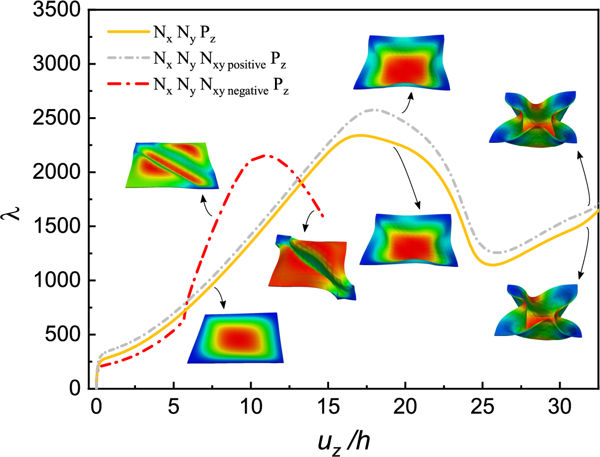
The equilibrium curves for this angle-ply composite plate subjected to different combined loadings are shown in Fig. 17, which plots the normalized values of the displacement in the middle point of the plate versus the normalized values of the applied compressive line load in the -axis direction. The horizontal lines in this figure display the corresponding linear buckling loads predicted by the CUF method. It is found from Fig. 17 that for this symmetric composite structure, the buckling loads predicted by the linear buckling analysis are almost the same as those based on CUF Full NL plate model, even if there exists uniform transverse pressure applied to the plate. Thus, the linear buckling analysis can be exploited to first predict the buckling load of the symmetric composite structure. In addition, the linear buckling load of the angle-ply plate with positive shear is higher than other loading cases, which demonstrates the previously mentioned fact that the angle-ply plate with positive shear loading has higher rigidity and load-carrying capacity. Finally, it is noted that as the transverse pressure is relatively small compared with the in-plane loads, the equilibrium curves with transverse pressure gradually approach those without transverse pressure when continuously increasing the loading.

3.2.4 Cross-ply [0/90] square laminate with different edge conditions
The effect of different plate edge conditions on the post-buckling nonlinear response of the cross-ply composite plate under in-plane compressive load is presented for the final post-buckling example. This problem deals with a cross-ply square plate with different edge conditions [30]. This 2D model has the width of m and the thickness of cm. In the first analysis case, the plate is subjected to a uniformly distributed in-plane compressive line load in the -axis direction , while in the second analysis case, the plate is subjected to a uniformly distributed in-plane compressive line load in the -axis direction . The edge conditions are SSSS, SSCC, SSSC, SSFC, and SSFS. The letters “S”, “C”, and “F” indicate simply-supported, clamped, and free edge conditions. It should be noted that the third and fourth letters of the boundary condition refer to and . Furthermore, the clamped edge conditions satisfy at the corresponding edge and the simply-supported edge conditions satisfy at , or at . Material properties for the bove-mentioned composite plate are shown in Table 15.
| E1 (GPa) | (GPa) | (GPa) | G23 (GPa) | |
|---|---|---|---|---|
| 220 | 5.5 | 3.3 | 2.75 | 0.25 |
For this cross-ply composite plate with simply-supported edge conditions, the convergence analysis of the equilibrium curves for the in-plane compressive loads in the -axis direction is provided in Fig. 18.

This figure shows that the convergence is obtained at least for the 1212Q9-LD1 plate model. The equilibrium curves based on this convergence plate model are investigated for SSSS, SSCC, SSSC, SSFC, and SSFS edge conditions in Figs. 19 and 20 to evaluate the effect of different edge conditions on the nonlinear response of the cross-ply composite plate. The horizontal lines in these two figures’ enlarged views indicate the corresponding linear buckling loads by the CUF method. The results show that the load-carrying capacity of the composite plate with the clamped edge conditions is higher than other investigated edge conditions. Furthermore, it can be understood that the presence of a free edge reduces the buckling strength significantly. The current method can also predict the nonlinear response of the composite plate beyond the limit load and the snap-through instability.


4 Conclusions
In this work, large deflection and post-buckling analyses of laminated composite plates have been investigated by employing the Carrera Unified Formulation (CUF) and the layerwise (LW) approach based on Lagrange expansion. The path-following Newton-Raphson linearization method has been adopted to compute the full geometrically nonlinear plate problems. Different two-dimensional (2D) composite plate structures subjected to large deflections/rotations and post-buckling have been analyzed and the numerical results have been compared with solutions in the available literature. Furthermore, the linear buckling load of the composite plates has been calculated for the post-buckling cases. The effects of different parameters, such as the stacking sequence, number of layers, loading way, and edge conditions, have been investigated and discussed in detail. The results have demonstrated that:
- •
The equilibrium curves obtained by the CUF linear and Full NL models agree well with those in the available literature or the ABAQUS 3D solid model solutions;
- •
Increasing the layer number of the composite plates results in the higher buckling strength and load-carrying capacity of the composite structures;
- •
For the angle-ply laminate subjected to the combined loading (in-plane shear and bi-axial compression), the direction of the applied shear plays a pivotal role in the post-buckling behaviour of the composite plate, and the angle-ply plate with positive shear loading shows higher rigidity and load-carrying capacity;
- •
The buckling strength and the load-carrying capacity of the composite plates with the clamped edge conditions are higher compared to other investigated edge conditions, and the presence of a free edge reduces the buckling strength significantly;
- •
The linear buckling analysis cannot be utilized to calculate the buckling load of the antisymmetric structure. However, the buckling loads predicted by the linear buckling analysis for symmetric composite structures are almost the same as those based on CUF Full NL plate model.
Further developments of the proposed methodology are being studied, such as a non-linear local analysis and a localized buckling with the advantage of coupling the global/local approach with optimization tools to reduce computation time. Furthermore, the same non-linear methodology will also be adopted to perform dynamic analyses. Another important topic under development is the use of CUF in civil problems, such as the analysis of reinforced concrete structures. The adoption of an LW approach for studying the nonlinear behaviour of the section once the concrete cracks have some potential and advantages on the accuracy of the results and processing times.
Declaration of competing interest
Authors declare that they have no known competing financial interests or personal relationships that could appear to influence the work reported in this paper.
Author contributions
E. Carrera: Conceptualization, Funding acquisition, Methodology. R. Azzara: Investigation, Visualization, Writing - original draft. E. Daneshkhah: Investigation, Visualization, Writing - original draft. A. Pagani: Supervision, Software, Writing - review editing. B. Wu: Visualization, Writing - review editing.
Acknowledgments
This work was supported by the European Union’s Horizon 2020 Research and Innovation Programme under the Marie Skłodowska-Curie Actions, Grant No. 896229 (B.W.).
References
- [1] A.K. Kaw. Mechanics of Composite Materials. CRC press, 2005.
- [2] M.R. Forouzan, E. Daneshkhah, et al. Damage and residual bending strength in glass-polyester molded grating composite panels after low-velocity impact. Composite Structures, 227:111290, 2019.
- [3] A. Pagani, E. Carrera, A. Hasanyan, and S. Pellegrino. Advanced simulation ant testing of composite TRAC longerons. In 71st International Astronautical Congress (IAC), pages 12–14, 2020.
- [4] P. Dash and B.N. Singh. Static response of geometrically nonlinear laminated composite plates having uncertain material properties. Mechanics of Advanced Materials and Structures, 22(4):269–280, 2015.
- [5] B.N. Singh, A. Lal, and R. Kumar. Nonlinear bending response of laminated composite plates on nonlinear elastic foundation with uncertain system properties. Engineering Structures, 30(4):1101–1112, 2008.
- [6] Y.X. Zhang and C.H. Yang. Recent developments in finite element analysis for laminated composite plates. Composite Structures, 88(1):147–157, 2009.
- [7] W. Han, M. Petyt, and K.M. Hsiao. An investigation into geometrically nonlinear analysis of rectangular laminated plates using the hierarchical finite element method. Finite Elements in Analysis and Design, 18(1-3):273–288, 1994.
- [8] Y.X. Zhang and K.S. Kim. A simple displacement-based 3-node triangular element for linear and geometrically nonlinear analysis of laminated composite plates. Computer Methods in Applied Mechanics and Engineering, 194(45-47):4607–4632, 2005.
- [9] Y.X. Zhang and K.S. Kim. Geometrically nonlinear analysis of laminated composite plates by two new displacement-based quadrilateral plate elements. Composite Structures, 72(3):301–310, 2006.
- [10] L.V. Tran, J. Lee, H. Nguyen-Van, H. Nguyen-Xuan, and M.A. Wahab. Geometrically nonlinear isogeometric analysis of laminated composite plates based on higher-order shear deformation theory. International Journal of Non-Linear Mechanics, 72:42–52, 2015.
- [11] C. Sridhar and K.P.. Rao. Large deformation finite element analysis of laminated circular composite plates. Computers & Structures, 54(1):59–64, 1995.
- [12] K.M. Liew, J. Wang, M.J. Tan, and S. Rajendran. Nonlinear analysis of laminated composite plates using the mesh-free kp-Ritz method based on FSDT. Computer Methods in Applied Mechanics and Engineering, 193(45-47):4763–4779, 2004.
- [13] F. Alijani and M. Amabili. Non-linear dynamic instability of functionally graded plates in thermal environments. International Journal of Non-Linear Mechanics, 50:109–126, 2013.
- [14] A.K. Baltacıoğlu, Ö. Civalek, B. Akgöz, and F. Demir. Large deflection analysis of laminated composite plates resting on nonlinear elastic foundations by the method of discrete singular convolution. International Journal of Pressure Vessels and Piping, 88(8-9):290–300, 2011.
- [15] B.S. Reddy, A.R. Reddy, J.S. Kumar, and K.V.K. Reddy. Bending analysis of laminated composite plates using finite element method. International Journal of Engineering, Science and Technology, 4(2):177–190, 2012.
- [16] J.N. Reddy. Mechanics of Laminated Composite Plates and Shells: Theory and Analysis. CRC press, 2003.
- [17] M. Gorji. On large deflection of symmetric composite plates under static loading. Proceedings of the Institution of Mechanical Engineers, Part C: Journal of Mechanical Engineering Science, 200(1):13–19, 1986.
- [18] Y. Zhang and F.L. Matthews. Large deflection behavior of simply supported laminated panels under in-plane loading. Journal of Applied Mechanics, 52(3):553–558, 1985.
- [19] M. Amabili. Nonlinear Vibrations and Stability of Shells and Plates. Cambridge University Press, New York, USA, 2008.
- [20] M. Amabili. Nonlinear Mechanics of Shells and Plates in Composite, Soft and Biological Materials. Cambridge University Press, New York, USA, 2018.
- [21] S. Hui-Shen. Buckling and postbuckling behavior of antisymmetrically angle-ply laminated composite plates. Applied Mathematics and Mechanics, 11(12):1155–1165, 1990.
- [22] S. Hui-shen. Postbuckling Behavior of Plates and Shells. World Scientific, 2017.
- [23] Y. Zhang and F.L. Matthews. Postbuckling behaviour of curved panels of generally layered composite materials. Composite Structures, 1(2):115–135, 1983.
- [24] P. Dash and B.N. Singh. Buckling and post-buckling of laminated composite plates. Mechanics Research Communications, 46:1–7, 2012.
- [25] A.W. Leissa. A review of laminated composite plate buckling. Applied Mechanics Reviews, 40(5):575–591, 1987.
- [26] G.J. Turvey and I.H. Marshall. Buckling and postbuckling of composite plates. Springer Science & Business Media, 2012.
- [27] L. Librescu and M. Stein. A geometrically nonlinear theory of transversely isotropic laminated composite plates and its use in the post-buckling analysis. Thin-Walled Structures, 11(1-2):177–201, 1991.
- [28] S.S. Wang, S. Srinivasan, H.T. Hu, and R. HajAli. Effect of material nonlinearity on buckling and postbuckling of fiber composite laminated plates and cylindrical shells. Composite Structures, 33(1):7–15, 1995.
- [29] P. Sundaresan, G. Singh, and G.V. Rao. Buckling and post-buckling analysis of moderately thick laminated rectangular plates. Computers & Structures, 61(1):79–86, 1996.
- [30] K.M. Liew, J. Wang, M.J. Tan, and S. Rajendran. Postbuckling analysis of laminated composite plates using the mesh-free kp-Ritz method. Computer Methods in Applied Mechanics and Engineering, 195(7-8):551–570, 2006.
- [31] M. Amabili and M.R.S. Tajahmadi. Thermal post-buckling of laminated and isotropic rectangular plates with fixed edges: Comparison of experimental and numerical results. Proceedings of the Institution of Mechanical Engineers, Part C: Journal of Mechanical Engineering Science, 226(10):2393–2401, 2012.
- [32] Q. Chen and P. Qiao. Post-buckling analysis of composite plates under combined compression and shear loading using finite strip method. Finite Elements in Analysis and Design, 83:33–42, 2014.
- [33] P. Dash and B.N. Singh. Buckling and post-buckling response of laminated composite plate with random system properties. Mechanics of Advanced Materials and Structures, 21(6):516–529, 2014.
- [34] A. Pagani and E. Carrera. Unified formulation of geometrically nonlinear refined beam theories. Mechanics of Advanced Materials and Structures, 25(1):15–31, 2018.
- [35] A. Pagani and E. Carrera. Large-deflection and post-buckling analyses of laminated composite beams by Carrera Unified Formulation. Composite Structures, 170:40–52, 2017.
- [36] B. Wu, A. Pagani, M. Filippi, W.Q. Chen, and E. Carrera. Accurate stress fields of post-buckled laminated composite beams accounting for various kinematics. International Journal of Non-Linear Mechanics, 111:60–71, 2019.
- [37] B. Wu, A. Pagani, M. Filippi, W.Q. Chen, and E. Carrera. Large-deflection and post-buckling analyses of isotropic rectangular plates by Carrera Unified Formulation. International Journal of Non-Linear Mechanics, 2019.
- [38] M. Petrolo, M.H. Nagaraj, I. Kaleel, and E. Carrera. A global-local approach for the elastoplastic analysis of compact and thin-walled structures via refined models. Computers & Structures, 206:54–65, 2018.
- [39] I. Kaleel, M. Petrolo, E. Carrera, and A.M. Waas. Computationally efficient concurrent multiscale framework for the nonlinear analysis of composite structures. AIAA Journal, 57(9):4029–4041, 2019.
- [40] I. Kaleel, M. Petrolo, E. Carrera, and A.M. Waas. On the effectiveness of higher-order one-dimensional models for physically nonlinear problems. pages 67–81, 2019.
- [41] E. Carrera. Multilayered shell theories accounting for layerwise mixed description, Part 1: governing equations. AIAA Journal, 37(9):1107–1116, 1999.
- [42] E. Carrera. Multilayered shell theories accounting for layerwise mixed description, Part 2: Numerical evaluations. AIAA Journal, 37(9):1117–1124, 1999.
- [43] A. Pagani, E. Carrera, and R. Augello. Evaluation of various geometrical nonlinearities in the response of beams and shells. AIAA Journal, 57(8):3524–3533, 2019.
- [44] A. Pagani, E. Daneshkhah, X. Xu, and E. Carrera. Evaluation of geometrically nonlinear terms in the large-deflection and post-buckling analysis of isotropic rectangular plates. International Journal of Non-Linear Mechanics, 121:103461, 2020.
- [45] E. Carrera, A. Pagani, R. Azzara, and R. Augello. Vibration of metallic and composite shells in geometrical nonlinear equilibrium states. Thin-Walled Structures, 157:107131, 2020.
- [46] B. Wu, A. Pagani, W.Q. Chen, and E. Carrera. Geometrically nonlinear refined shell theories by Carrera Unified Formulation. Mechanics of Advanced Materials and Structures, pages 1–21, 2019.
- [47] A. Pagani, R. Azzara, R. Augello, E. Carrera, and B. Wu. Accurate through-the-thickness stress distributions in thin-walled metallic structures subjected to large displacements and large rotations. Vietnam Journal of Mechanics, 42(3):239–254, 2020.
- [48] K. J. Bathe. Finite Element Procedure. Prentice Hall, Upper Saddle River, New Jersey, USA, 1996.
- [49] O.O. Ochoa and J.N. Reddy. Finite element analysis of composite laminates. In Finite Element Analysis of Composite Laminates, pages 37–109. Springer, 1992.
- [50] E. Carrera, M. Cinefra, M. Petrolo, and E. Zappino. Finite Element Analysis of Structures through Unified Formulation. John Wiley & Sons, Chichester, West Sussex, UK, 2014.
- [51] E. Carrera, A. Pagani, and M. Petrolo. Classical, refined and component-wise theories for static analysis of reinforced-shell wing structures. AIAA Journal, 51(5):1255–1268, 2013.
- [52] E. Carrera and A. Pagani. Accurate response of wing structures to free vibration, load factors and non-structural masses. AIAA Journal, 54(1):227–241, 2016.
- [53] E. Carrera and A. Pagani. Free vibration analysis of civil engineering structures by component-wise models. Journal of Sound and Vibration, 333(19):4597–4620, 2014.
- [54] M.A. Crisfield. Non-linear Finite Eelement Analysis of Solid and Structures. John Wiley & Sons, 1991.
- [55] S.C. Han, S.Y. Lee, and G. Rus. Postbuckling analysis of laminated composite plates subjected to the combination of in-plane shear, compression and lateral loading. International Journal of Solids and Structures, 43(18-19):5713–5735, 2006.
- [56] S.J. Lee and W. Kanok-Nukulchai. A nine-node assumed strain finite element for large-deformation analysis of laminated shells. International Journal for Numerical Methods in Engineering, 42(5):777–798, 1998.
- [57] A.K. Noor and M.D. Mathers. Anisotropy and shear deformation in laminated composite plates. AIAA Journal, 14(2):282–285, 1976.