Universal Inflationary Attractors Implications on Static Neutron Stars
Abstract
We study static neutron stars in the context of a class of non-minimally coupled inflationary potentials, the universal attractors. Universal attractors are known to generate a viable inflationary era, and they fall into the same category of inflationary phenomenology as the model and other well-known cosmological attractors. We present the essential features of universal attractors in both the Einstein and Jordan frame, and we extract the Tolman-Oppenheimer-Volkoff equations in the Einstein frame using the usual notation of theoretical astrophysics. We use a python 3 based double shooting numerical code for our numerical analysis and we construct the graphs for the universal attractor potential, using piecewise polytropic equation of state the small density part of which is the WFF1 or the APR or the SLy equation of state. As we show, all the studied cases predict larger maximum masses for the neutron stars, and all the results are compatible with the GW170817 constraints imposed on the radii of the neutron stars.
pacs
04.50.Kd, 95.36.+x, 98.80.-k, 98.80.Cq,11.25.-wIntroduction
The last three decades have brought cosmology and astrophysics to the mainstream of physics, since the observation of dark energy Riess:1998cb and the direct detection of gravitational waves TheLIGOScientific:2017qsa; Abbott:2020khf have altered the way of thinking on how the Universe works in small and large scales. Neutron stars (NS) Haensel:2007yy; Friedman:2013xza; Baym:2017whm; Lattimer:2004pg; Olmo:2019flu currently are in the interest of many scientific areas, like nuclear theory Lattimer:2012nd; Steiner:2011ft; Horowitz:2005zb; Watanabe:2000rj; Shen:1998gq; Xu:2009vi; Hebeler:2013nza; Mendoza-Temis:2014mja; Ho:2014pta; Kanakis-Pegios:2020kzp,, high energy physics Buschmann:2019pfp; Safdi:2018oeu; Hook:2018iia; Edwards:2020afl; Nurmi:2021xds, modified gravity Astashenok:2020qds; Astashenok:2021peo; Capozziello:2015yza; Astashenok:2014nua; Astashenok:2014pua; Astashenok:2013vza; Arapoglu:2010rz; Panotopoulos:2021sbf; Lobato:2020fxt and astrophysics Bauswein:2020kor; Vretinaris:2019spn; Bauswein:2020aag; Bauswein:2017vtn; Most:2018hfd; Rezzolla:2017aly; Nathanail:2021tay; Koppel:2019pys.
There is strong evidence coming from the observations on dark energy that modified gravity in its various forms Nojiri:2017ncd; Nojiri:2009kx; Capozziello:2011et; Capozziello:2010zz; Nojiri:2006ri; Nojiri:2010wj; delaCruzDombriz:2012xy; Olmo:2011uz actually plays a fundamental role on large scales. Also at the astrophysical level, it is possible to generate large or extremely large neutron star masses and solve several fundamental equation of state (EoS) related problems of neutron stars Astashenok:2014nua; Astashenok:2014pua. Hence it is probable that general relativity (GR) by itself may not suffice to describe NSs, hence some extension of GR might be compelling. In this work we shall consider NSs in hydrodynamic equilibrium in the context of non-minimally coupled scalar-tensor theories. This subject is very well studied in the theoretical astrophysics literature, see Refs. Pani:2014jra; Staykov:2014mwa; Horbatsch:2015bua; Silva:2014fca; Doneva:2013qva; Xu:2020vbs; Salgado:1998sg; Shibata:2013pra; Arapoglu:2019mun; Ramazanoglu:2016kul; AltahaMotahar:2019ekm; Chew:2019lsa; Blazquez-Salcedo:2020ibb; Motahar:2017blm for an important stream of articles on this subject. We shall consider some not so well known in the theoretical astrophysics literature non-minimal coupled theories, those of cosmological attractors alpha1; alpha2; alpha3; alpha4; alpha5; alpha6; alpha7; alpha7a; alpha8; alpha9; alpha10; alpha11; alpha12; alpha13; alpha14; alpha15; alpha16; alpha17; alpha18; alpha19; alpha20; alpha21; alpha22; alpha23; alpha24; alpha25; alpha26; alpha27; alpha28; alpha29; alpha30; alpha31; alpha32; alpha33; alpha34; alpha35; alpha36; alpha37. Specifically, in this work we shall consider the class known as universal attractors alpha7a, and we shall investigate the implications of such non-minimally coupled scalar field theories on static NSs in the Einstein frame. These models are known to provide a uniform inflationary phenomenology and belong to the larger class of cosmological attractors, which provide a viable inflationary phenomenology compatible with the latest Planck data Akrami:2018odb. We shall solve numerically the Tolman-Oppenheimer-Volkoff (TOV) equations, using an “LSODA” integrator python 3 based code, which is a modification of niksterg, and with regard to the EoS for the nuclear matter, we shall assume that the EoS is a piecewise polytropic EoS Read:2008iy; Read:2009yp, with the low density part being the WFF1 Wiringa:1988tp, the SLy Douchin:2001sv, of the APR EoS Akmal:1998cf. With regard to the mass of the NS, we shall find the numerical value of the Einstein frame Arnowitt-Deser-Misner (ADM) mass Arnowitt:1960zzc and from it we shall calculate the Jordan frame mass numerically.
This paper is organized as follows: In section I we review the essential features of the universal attractors in the context of cosmology, and we shall demonstrate how these models provide a viable inflationary era. In section II we discuss these models in the context of theoretical astrophysics notation and physical units, and we solve numerically the TOV equations for the three distinct EoSs. In the same section we qualitatively discuss the phenomenological features of the NSs for the universal attractor potentials. Finally the conclusions follow in the end of the paper.
I Essential Features of Universal Attractor Theories
Universal attractors belong to a large class of cosmological attractors studied in Refs. alpha1; alpha2; alpha3; alpha4; alpha5; alpha6; alpha7; alpha7a; alpha8; alpha9; alpha10; alpha11; alpha12; alpha13; alpha14; alpha15; alpha16; alpha17; alpha18; alpha19; alpha20; alpha21; alpha22; alpha23; alpha24; alpha25; alpha26; alpha27; alpha28; alpha29; alpha30; alpha31; alpha32; alpha33; alpha34; alpha35; alpha36; alpha37. All these cosmological attractor models originate from various forms of Jordan frame non-minimally coupled scalar theories, but the Einstein frame counterpart yield a quite similar inflationary phenomenology, for generic non-minimal coupling. In this section we shall briefly demonstrate how the universal attractors inflationary theory is obtained. The notation we shall use is frequently used in cosmological contexts, so we use natural units for this section. In the next section where we study the Einstein frame NS phenomenology, we switch to Geometrized units. The conventions and formalism of conformal transformations in cosmological contexts, we refer the reader to Refs. Kaiser:1994vs; valerio.
We start of with the Jordan frame action of a non-minimally coupled scalar field ,
| (1) |
with denoting the Jordan frame perfect matter fluids, with and energy density . The universal attractors in the Jordan frame have the following non-minimal coupling,
| (2) |
where is a positive constant coupling, and the reduced Planck mass is defined as follows,
| (3) |
where is the gravitational constant of Newtonian gravity. Moreover, the universal attractors in the Jordan frame have the following scalar potential,
| (4) |
with being some positive number. Now if the following conformal transformation is performed in the Jordan frame action with metric ,
| (5) |
we obtain the Einstein frame action with metric , where the “tilde” will denote the Einstein frame quantities. If we use Kaiser:1994vs; valerio,
| (6) |
we may obtain a minimal coupled scalar theory in the Einstein frame,
| (7) |
where,
| (8) |
and the potential is written in terms of the Jordan frame potential as,
| (9) |
thus in view of Eqs. (10) and (9), the Einstein frame potential for the universal attractors reads,
| (10) |
The Einstein frame scalar field can be made canonical by using the following transformation,
| (11) |
hence the Einstein frame action becomes,
| (12) |
The Einstein frame matter fluids are coupled to the conformal factor so these are not perfect, because the energy momentum tensor satisfies,
| (13) |
Hereafter we shall assume that,
| (14) |
which by using the analytic form of for the universal attractors, the above condition can be written as follows,
| (15) |
By substituting the analytic form of from Eq. (2) into Eq. (8), we have,
| (16) |
so in view of the assumption (14), we easily obtain from Eq. (16) the following,
| (17) |
or equivalently,
| (18) |
Hence, by substituting Eq. (18) in Eq. (10) we finally obtain the Einstein frame scalar potential in terms of the canonical scalar field ,
| (19) |
Let us set for convenience , and by taking into the Planck constraints Akrami:2018odb on the amplitude of single canonical scalar field fluctuations,
| (20) |
where is,
| (21) |
the parameter is constrained to be,
| (22) |
Let us elaborate further on the constraint we just quoted, namely the parameter . This parameter is constrained by the Planck data in a model independent way, using the BK15 constraint on (which is ), see for example Eq. (32) of the Planck 2018 constraints on inflation, page 14 Akrami:2018odb. In that equation the tensor-to-scalar ratio is used, while we replaced in Eq. (21). Also note that in our notation the amplitude of the scalar fluctuations is while in the Planck data this is denoted as . Therefore the constraint of Eq. (32) of Ref. Akrami:2018odb is equivalent to our constraint (upper bound) Eq. (20), which if we substitute the maxim allowed values of the slow-roll index (or equivalently the maximum allowed value of the tensor-to-scalar ratio), we obtain the constraint (22) of our paper. This is obtained in a general and model-independent way and does not rely on the specifics of the model used, it is solely based on the Planck constraints on canonical scalar field inflation.
Clearly the constraint on is an upper bound and we thus focused on this upper bound case in our paper. Definitely the parameter can take smaller values, but we used the upper bounds values for the slow-roll parameters and , thus we focused our analysis on the maximum value for the scale of inflation . In principle one could use lower values for the scale of inflation, until for example GeV, which is the low-scale inflation constraint (we used the slow-roll relation ), but this would not change drastically the parameter , plus one should explain how the low-scale inflation scenario occurs. Hence in our approach we used the most plausible values for the scale of inflation, inherently connected to the ordinary scale of inflation, not the low-scale of inflation.
Note that and in Eq. (21) are the value of the canonical scalar field in the Einstein frame at the end of inflation and the first slow-roll index. The canonical scalar theory in the Einstein frame with the potential (19), which has a resulting action in the Einstein frame,
| (23) |
yields a viable inflationary phenomenology and has an attractor behavior resulting to the following spectral index of primordial scalar curvature perturbations and tensor-to-scalar ratio, at leading order in the large -foldings number ,
| (24) |
The above observational indices for inflation are identical to the ones corresponding to the model and other inflationary phenomenological models. A useful expression for the action (23) is the following,
| (25) |
and recall that . The above form of the action is convenient for the universal attractor theory in the Einstein frame in the context of theoretical astrophysics notation. Also let us comment that the action (23) us identical to the one corresponding to the model for , and this is the case we shall also study. However, the two theories yield only identical inflation but the two theories are not the same because the conformal factor and the resulting coupling to the matter fluids are not the same, so these two theories look like the same but are not the same. We evince this feature in the next section.
II Neutron Stars in the Einstein Frame with Universal Attractors
Let us now study the universal attractor potentials in astrophysical contexts. We shall use Geometrized units , and also we adopt the notation and conventions of Ref. Pani:2014jra. The Jordan frame action of a non-minimally coupled scalar field in the presence of perfect matter fluids is,
| (26) |
By conformally transforming the above action using,
| (27) |
we obtain the Einstein frame action which is,
| (28) |
where is the Einstein frame canonical scalar field, which is related to the scalar field as follows,
| (29) |
while the potential is,
| (30) |
Now the universal attractors case corresponds to the choices,
| (31) |
and for these choices, Eq. (29) becomes,
| (32) |
Now, for the case and notation at hand, the assumption of Eq. (14) reads,
| (33) |
and in view of this assumption, we can integrate Eq. (29) to obtain,
| (34) |
and now due to Eq. (27) the conformal factor reads,
| (35) |
In addition, a useful quantity which shall be used in the following is the function defined as follows,
| (36) |
hence in the case of universal attractors,
| (37) |
It is worth noting that when then , thus at this limit the Einstein and Jordan frame are not equivalent, see for example Bhattacharya:2020wdl, however we do not have to worry for this limit, since during inflation, the values of the scalar field are of the order of the Planck mass, while even at astrophysical contexts, such as interior and exterior of scalar-tensor neutron stars, the values of the scalar field are significantly smaller than the Planck mass. Also, using (34) and (37) the potential in the Einstein frame takes the final form,
| (38) |
where . From this point we shall assume that , thus let us use the constraints on from the previous section to determine the values of always working in Geometrized units with . By comparing the actions (25) and (38), we have , so . Hence, since , we can choose and , and we can observe that for this choice we shall also explicitly check whether the constraint (33) holds true, in the Jordan frame.

We shall consider static NSs in the Einstein frame. Thus, the spherically symmetric static metric which describes the NS used in this paper is,
| (39) |
where the function stands for the gravitational mass of the NS with circumferential radius . It is worth discussing here the issue of exterior and interior spacetime for the static neutron star. In standard GR contexts where the scalar field is absent, the exterior spacetime of the neutron star is Schwarzschild, however in the presence of the scalar field the spacetime is uniformly given by the metric (39), see for example Pani:2014jra. It is the aim of any study in scalar-tensor astrophysics to find, numerically, the metric functions and . Obviously no matching conditions are required at the surface of the star, because the TOV equations will yield a continuous solution for the metric functions, starting from the interior of the star, extending to the surface of the star and these solutions will describe the star asymptotically, thus at . At exactly this point, the numerical infinity, the exterior spacetime will be a Schwarzschild spacetime, and this is the only condition imposed on the metric functions and . These have to be matched with the corresponding Schwarzschild ones. The solutions for the metric functions and will be obtained numerically by solving the TOV equations continuously from the interior until the numerical infinity. The difference between the interior of the star and the exterior is that the exterior does not have contribution from the matter of the star, thus the pressure and the energy density outside the star are zero. However, the potential is not switched off, thus it affects the metric function solutions even outside the star. This is the major difference of scalar-tensor gravity and GR for astrophysical compact objects. For the numerical procedure, it is important to match the metric function solutions asymptotically with the Schwarzschild ones, and thus a double shooting method is required for this, in order to find the optimal initial conditions at the center of the star which guarantee that the spacetime asymptotically will be matched with the Schwarzschild. The double shooting method we used guarantees that the spacetime at numerical infinity is Schwarzschild. Now we can derive the TOV equations, which are Pani:2014jra,
| (40) |
| (41) |
| (42) |
| (43) |
| (44) |
with the function is defined in Eq. (37). Note that the pressure and the energy density and , are Jordan frame quantities. Also the interior and the interior spacetime are uniformly described by the metric (39), no discrimination to exterior and interior spacetimes is done here, like in GR. The TOV equations for the spacetime outside the star can be derived by setting and , which shows the absence of matter outside the star. However, the potential is still present thus it affects the star beyond its surface. This is exactly why no matching outside the star is needed at the surface. The numerical solutions of the TOV equations will yield continuous uniform solutions for the metric functions, and the only condition required is that asymptotically, these solutions must become identical to the corresponding Schwarzschild ones.
The initial conditions for the TOV equations are,
| (45) |
The condition means that the gravitational mass for zero radius is zero. This however does not make the metric function to be non-zero at zero radius. The exact value will be obtained by the double shooting method. With regard to the EoS, we shall use a piecewise polytropic EoS Read:2008iy; Read:2009yp (see also niksterg), with the low density parameters corresponding to the SLy, WFF1 or the APR EoSs. For the piecewise polytropic EoS, the relation between the energy density and pressure is,
| (46) |
where the refers to the three different pieces of the polytropic equation of state. Let us elaborate on this further, the energy density and the pressure in each of the three piecewise density intervals satisfy the polytropic relation,
| (47) |
and we only have to require that continuity is needed at the crossing points of each of the three pieces. Particularly, at the crossing points we must have,
| (48) |
and from the above relations, the parameters and are obtained, given , or equivalently, given the initial pressure and for given parameters , and , which are not chosen arbitrarily. Upon integrating the first thermodynamic law for barotropic fluids,
| (49) |
in conjunction with the continuity requirement at each piece of the polytropic, yields Eq. (46). Now let us discuss the gravitational mass issue for the NS. The gravitational mass of the NS which we shall consider is the ADM mass in the Jordan frame. Thus when we extract the numerical results, we need to transform the obtained Einstein frame mass to the Jordan frame. We define the auxiliary functions and in Geometrized units,
| (50) |
which are basically the metric functions in the Einstein and Jordan frames, with and being the gravitational mass confined in a radius . The metric functions along with the metric radius parameter in the two frames are related as follows,
| (51) |
and in addition, the Jordan and Einstein frame ADM masses are,
| (52) |
Taking the asymptotic limit of Eq. (51), we obtain,
| (53) |
where denotes the radius in the Einstein frame asymptotically (not at the numerical infinity though, slightly smaller) and in addition . Upon combining Eqs. (50)-(53) we acquire Odintsov:2021qbq,
| (54) |
Finally, the Jordan and Einstein frame radii of the NS are related as follows,
| (55) |
Hereafter we shall identify with the Jordan frame mass of Eq. (54), that is measured in solar masses, and the radius in the Jordan frame shall be expressed in kilometers.

At this point we shall proceed to the presentation of our numerical analysis of the TOV equations. We shall solve the TOV equations numerically using a python 3 based numerical code which is a variant form of the pyTOV-STT code niksterg using the “LSODA” integrator, in order to extract the Jordan frame mass and the circumferential radius of the NS. The method includes a double shooting method in order to find the optimal values for the the metric function and for the scalar field at the center of the NS, which make the values of the scalar field and of the metric function to vanish at the numerical infinity, with the latter being chosen in kilometers to be km.
| Model | APR EoS | SLy EoS | WFF1 EoS |
|---|---|---|---|
| GR | |||
| GR | km | km | km |
| Universal Attractors | |||
| Universal Attractors Radii | km | km | km |
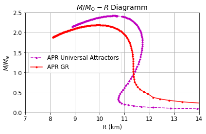
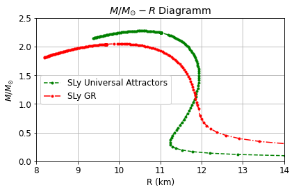
In Fig. 1 we present the graphs of the universal attractor models when compared to the corresponding GR curves, for the WFF1 EoS (upper), for the APR EoS (middle) and for the SLy EoS (bottom plot). In order to produce Fig. 1 we numerically solved the TOV equations and we extracted the masses and radii corresponding to 160 central densities, namely and and then we generated the graph using the resulting values for the mass and radii for each of these 160 central densities. Also in Fig. 2 we compare the universal attractors curves, for the three distinct EoSs. A first interesting result is that the WFF1 EoS for the universal attractor model is compatible with the GW170817 constraint derived in Ref. Bauswein:2017vtn, which indicates that NSs must have radii in the range km. This is in contrast to the GR case, where the WFF1 EoS is excluded by the GW170817 data. Secondly, in all the studied cases, the maximum mass NS configurations for the three distinct EoSs, satisfy the second constraint of GW170817 derived in Ref. Bauswein:2017vtn, which indicates that the maximum mass configurations must have radii larger than km. Also in Table 1 we present the radii of the static NS for all the EoS in both GR and the universal attractors models, for which . Note that the limit is never reached by the neutron stars, because these are GR objects bound from gravity solely even in the context of scalar-tensor gravity. In contrast, strange stars could reach the limit of very small radii. Furthermore, in Table 2 we gather the data for the maximum masses and the corresponding radii, for the GR NS and the universal attractors NS, and for all the EoSs studied in this paper.
| Model | APR EoS | SLy EoS | WFF1 EoS |
|---|---|---|---|
| GR | |||
| Universal Attractors | |||
| Universal Attractors Radii | km | km | km |
Finally, we need to explicitly check whether the approximation of Eq. (33), and in Fig. 3 we present the fraction of and of versus the central densities, for the three distinct EoSs, and for the values of the scalar field at the surface of the star. As it can be seen, the constraint of Eq. (33) is safely satisfied for the values of the parameter we used in this article. Also for brevity we did not include the case for the values of the scalar field at the center of the star, in which case the approximation of Eq. (33) is satisfied.


Concluding Remarks
In this paper we studied the phenomenology of NSs for universal attractor non-minimally coupled scalar theories of inflation. The universal attractors are known in cosmological contexts since these provide a viable inflationary era and also belong to a larger class of cosmological attractors that are similar to the inflation. We investigated how the universal attractors can be obtained in the strong coupling limit, that is for large , so the large coupling limit constraint must be satisfied by the resulting values of the scalar field in the Einstein frame. After demonstrating the essential features of the universal attractor theories, we used the theoretical astrophysics context and we found all the quantities that are involved in the Einstein frame TOV equations. We solved numerically the TOV equations using a double shooting method of a python 3 code, and we constructed the graphs for all the different EoS we studied. The resulting numerical values for the masses and radii of the NSs were the Jordan frame ones, calculated from the resulting Einstein frame quantities delivered by the numerical code. The results of our analysis are interesting since we demonstrated that the WFF1 EoS which was excluded by the GW170817 data in the context of GR, it is not anymore excluded for the universal attractors model, since for a NS of mass , the predicted radii for the universal attractor models are larger than km. Also all the three distinct EoS for the universal attractor models, predict higher maximum radii compared to the GR ones, and moreover all the radii respect the constraint of the GW170817 event which indicates that the radii corresponding to the maximum masse must be larger than km. A crucial issue we did not address is related to the question whether the attractor property satisfied by the inflationary theories, is also satisfied by the NSs. Work is in progress in this line of research.
Finally, let us comment that the inflationary era obviously has no effect on the neutron stars for the universal attractor potential. Obviously the two eras are not connected, since the scalar field value during inflation is much larger compared to the values of the scalar field in and outside of the neutron star. The only constraint coming from the inflationary era is on the parameter , the constant coupling of the scalar potential, and this is required satisfy Eq. (22).
Acknowledgments
I am indebted to N. Stergioulas and his MSc student Vaggelis Smyrniotis for the many hours spend on neutron star physics discussions and for sharing his professional knowledge on numerical integration of neutron stars in python.
References
- (1) A. G. Riess et al. [Supernova Search Team], Astron. J. 116 (1998), 1009-1038 doi:10.1086/300499 [arXiv:astro-ph/9805201 [astro-ph]].
- (2) B. P. Abbott et al. [LIGO Scientific and Virgo], Phys. Rev. Lett. 119 (2017) no.16, 161101 doi:10.1103/PhysRevLett.119.161101 [arXiv:1710.05832 [gr-qc]].
- (3) R. Abbott et al. [LIGO Scientific and Virgo], Astrophys. J. Lett. 896 (2020) no.2, L44 doi:10.3847/2041-8213/ab960f [arXiv:2006.12611 [astro-ph.HE]].
- (4) P. Haensel, A. Y. Potekhin and D. G. Yakovlev, Astrophys. Space Sci. Libr. 326 (2007), pp.1-619 doi:10.1007/978-0-387-47301-7
- (5) J. L. Friedman and N. Stergioulas, doi:10.1017/CBO9780511977596
- (6) G. Baym, T. Hatsuda, T. Kojo, P. D. Powell, Y. Song and T. Takatsuka, Rept. Prog. Phys. 81 (2018) no.5, 056902 doi:10.1088/1361-6633/aaae14 [arXiv:1707.04966 [astro-ph.HE]].
- (7) J. M. Lattimer and M. Prakash, Science 304 (2004), 536-542 doi:10.1126/science.1090720 [arXiv:astro-ph/0405262 [astro-ph]].
- (8) G. J. Olmo, D. Rubiera-Garcia and A. Wojnar, Phys. Rept. 876 (2020), 1-75 doi:10.1016/j.physrep.2020.07.001 [arXiv:1912.05202 [gr-qc]].
- (9) J. M. Lattimer, Ann. Rev. Nucl. Part. Sci. 62 (2012), 485-515 doi:10.1146/annurev-nucl-102711-095018 [arXiv:1305.3510 [nucl-th]].
- (10) A. W. Steiner and S. Gandolfi, Phys. Rev. Lett. 108 (2012), 081102 doi:10.1103/PhysRevLett.108.081102 [arXiv:1110.4142 [nucl-th]].
- (11) C. J. Horowitz, M. A. Perez-Garcia, D. K. Berry and J. Piekarewicz, Phys. Rev. C 72 (2005), 035801 doi:10.1103/PhysRevC.72.035801 [arXiv:nucl-th/0508044 [nucl-th]].
- (12) G. Watanabe, K. Iida and K. Sato, Nucl. Phys. A 676 (2000), 455-473 [erratum: Nucl. Phys. A 726 (2003), 357-365] doi:10.1016/S0375-9474(00)00197-4 [arXiv:astro-ph/0001273 [astro-ph]].
- (13) H. Shen, H. Toki, K. Oyamatsu and K. Sumiyoshi, Nucl. Phys. A 637 (1998), 435-450 doi:10.1016/S0375-9474(98)00236-X [arXiv:nucl-th/9805035 [nucl-th]].
- (14) J. Xu, L. W. Chen, B. A. Li and H. R. Ma, Astrophys. J. 697 (2009), 1549-1568 doi:10.1088/0004-637X/697/2/1549 [arXiv:0901.2309 [astro-ph.SR]].
- (15) K. Hebeler, J. M. Lattimer, C. J. Pethick and A. Schwenk, Astrophys. J. 773 (2013), 11 doi:10.1088/0004-637X/773/1/11 [arXiv:1303.4662 [astro-ph.SR]].
- (16) J. de Jesús Mendoza-Temis, M. R. Wu, G. Martínez-Pinedo, K. Langanke, A. Bauswein and H. T. Janka, Phys. Rev. C 92 (2015) no.5, 055805 doi:10.1103/PhysRevC.92.055805 [arXiv:1409.6135 [astro-ph.HE]].
- (17) W. C. G. Ho, K. G. Elshamouty, C. O. Heinke and A. Y. Potekhin, Phys. Rev. C 91 (2015) no.1, 015806 doi:10.1103/PhysRevC.91.015806 [arXiv:1412.7759 [astro-ph.HE]].
- (18) A. Kanakis-Pegios, P. S. Koliogiannis and C. C. Moustakidis, [arXiv:2012.09580 [astro-ph.HE]].
- (19) M. Buschmann, R. T. Co, C. Dessert and B. R. Safdi, Phys. Rev. Lett. 126 (2021) no.2, 021102 doi:10.1103/PhysRevLett.126.021102 [arXiv:1910.04164 [hep-ph]].
- (20) B. R. Safdi, Z. Sun and A. Y. Chen, Phys. Rev. D 99 (2019) no.12, 123021 doi:10.1103/PhysRevD.99.123021 [arXiv:1811.01020 [astro-ph.CO]].
- (21) A. Hook, Y. Kahn, B. R. Safdi and Z. Sun, Phys. Rev. Lett. 121 (2018) no.24, 241102 doi:10.1103/PhysRevLett.121.241102 [arXiv:1804.03145 [hep-ph]].
- (22) T. D. P. Edwards, B. J. Kavanagh, L. Visinelli and C. Weniger, [arXiv:2011.05378 [hep-ph]].
- (23) S. Nurmi, E. D. Schiappacasse and T. T. Yanagida, [arXiv:2102.05680 [hep-ph]].
- (24) A. V. Astashenok, S. Capozziello, S. D. Odintsov and V. K. Oikonomou, Phys. Lett. B 811 (2020), 135910 doi:10.1016/j.physletb.2020.135910 [arXiv:2008.10884 [gr-qc]].
- (25) A. V. Astashenok, S. Capozziello, S. D. Odintsov and V. K. Oikonomou, [arXiv:2103.04144 [gr-qc]].
- (26) S. Capozziello, M. De Laurentis, R. Farinelli and S. D. Odintsov, Phys. Rev. D 93 (2016) no.2, 023501 doi:10.1103/PhysRevD.93.023501 [arXiv:1509.04163 [gr-qc]].
- (27) A. V. Astashenok, S. Capozziello and S. D. Odintsov, JCAP 01 (2015), 001 doi:10.1088/1475-7516/2015/01/001 [arXiv:1408.3856 [gr-qc]].
- (28) A. V. Astashenok, S. Capozziello and S. D. Odintsov, Phys. Rev. D 89 (2014) no.10, 103509 doi:10.1103/PhysRevD.89.103509 [arXiv:1401.4546 [gr-qc]].
- (29) A. V. Astashenok, S. Capozziello and S. D. Odintsov, JCAP 12 (2013), 040 doi:10.1088/1475-7516/2013/12/040 [arXiv:1309.1978 [gr-qc]].
- (30) A. S. Arapoglu, C. Deliduman and K. Y. Eksi, JCAP 07 (2011), 020 doi:10.1088/1475-7516/2011/07/020 [arXiv:1003.3179 [gr-qc]].
- (31) G. Panotopoulos, T. Tangphati, A. Banerjee and M. K. Jasim, [arXiv:2104.00590 [gr-qc]].
- (32) R. Lobato, O. Lourenço, P. H. R. S. Moraes, C. H. Lenzi, M. de Avellar, W. de Paula, M. Dutra and M. Malheiro, JCAP 12 (2020), 039 doi:10.1088/1475-7516/2020/12/039 [arXiv:2009.04696 [astro-ph.HE]].
- (33) A. Bauswein, G. Guo, J. H. Lien, Y. H. Lin and M. R. Wu, [arXiv:2012.11908 [astro-ph.HE]].
- (34) S. Vretinaris, N. Stergioulas and A. Bauswein, Phys. Rev. D 101 (2020) no.8, 084039 doi:10.1103/PhysRevD.101.084039 [arXiv:1910.10856 [gr-qc]].
- (35) A. Bauswein, S. Blacker, V. Vijayan, N. Stergioulas, K. Chatziioannou, J. A. Clark, N. U. F. Bastian, D. B. Blaschke, M. Cierniak and T. Fischer, Phys. Rev. Lett. 125 (2020) no.14, 141103 doi:10.1103/PhysRevLett.125.141103 [arXiv:2004.00846 [astro-ph.HE]].
- (36) A. Bauswein, O. Just, H. T. Janka and N. Stergioulas, Astrophys. J. Lett. 850 (2017) no.2, L34 doi:10.3847/2041-8213/aa9994 [arXiv:1710.06843 [astro-ph.HE]].
- (37) E. R. Most, L. R. Weih, L. Rezzolla and J. Schaffner-Bielich, Phys. Rev. Lett. 120 (2018) no.26, 261103 doi:10.1103/PhysRevLett.120.261103 [arXiv:1803.00549 [gr-qc]].
- (38) L. Rezzolla, E. R. Most and L. R. Weih, Astrophys. J. Lett. 852 (2018) no.2, L25 doi:10.3847/2041-8213/aaa401 [arXiv:1711.00314 [astro-ph.HE]].
- (39) A. Nathanail, E. R. Most and L. Rezzolla, Astrophys. J. Lett. 908 (2021) no.2, L28 doi:10.3847/2041-8213/abdfc6 [arXiv:2101.01735 [astro-ph.HE]].
- (40) S. Köppel, L. Bovard and L. Rezzolla, Astrophys. J. Lett. 872 (2019) no.1, L16 doi:10.3847/2041-8213/ab0210 [arXiv:1901.09977 [gr-qc]].
- (41) S. Nojiri, S. D. Odintsov and V. K. Oikonomou, Phys. Rept. 692 (2017) 1 doi:10.1016/j.physrep.2017.06.001 [arXiv:1705.11098 [gr-qc]].
- (42) S. Nojiri, S. D. Odintsov and D. Saez-Gomez, Phys. Lett. B 681 (2009) 74 doi:10.1016/j.physletb.2009.09.045 [arXiv:0908.1269 [hep-th]].
- (43) S. Capozziello and M. De Laurentis, Phys. Rept. 509 (2011) 167 doi:10.1016/j.physrep.2011.09.003 [arXiv:1108.6266 [gr-qc]].
- (44) V. Faraoni and S. Capozziello, Fundam. Theor. Phys. 170 (2010). doi:10.1007/978-94-007-0165-6
- (45) S. Nojiri and S. D. Odintsov, eConf C 0602061 (2006) 06 [Int. J. Geom. Meth. Mod. Phys. 4 (2007) 115] doi:10.1142/S0219887807001928 [hep-th/0601213].
- (46) S. Nojiri and S. D. Odintsov, Phys. Rept. 505 (2011) 59 doi:10.1016/j.physrep.2011.04.001 [arXiv:1011.0544 [gr-qc]].
- (47) A. de la Cruz-Dombriz and D. Saez-Gomez, Entropy 14 (2012) 1717 doi:10.3390/e14091717 [arXiv:1207.2663 [gr-qc]].
- (48) G. J. Olmo, Int. J. Mod. Phys. D 20 (2011) 413 doi:10.1142/S0218271811018925 [arXiv:1101.3864 [gr-qc]].
- (49) P. Pani and E. Berti, Phys. Rev. D 90 (2014) no.2, 024025 doi:10.1103/PhysRevD.90.024025 [arXiv:1405.4547 [gr-qc]].
- (50) K. V. Staykov, D. D. Doneva, S. S. Yazadjiev and K. D. Kokkotas, JCAP 10 (2014), 006 doi:10.1088/1475-7516/2014/10/006 [arXiv:1407.2180 [gr-qc]].
- (51) M. Horbatsch, H. O. Silva, D. Gerosa, P. Pani, E. Berti, L. Gualtieri and U. Sperhake, Class. Quant. Grav. 32 (2015) no.20, 204001 doi:10.1088/0264-9381/32/20/204001 [arXiv:1505.07462 [gr-qc]].
- (52) H. O. Silva, C. F. B. Macedo, E. Berti and L. C. B. Crispino, Class. Quant. Grav. 32 (2015), 145008 doi:10.1088/0264-9381/32/14/145008 [arXiv:1411.6286 [gr-qc]].
- (53) D. D. Doneva, S. S. Yazadjiev, N. Stergioulas and K. D. Kokkotas, Phys. Rev. D 88 (2013) no.8, 084060 doi:10.1103/PhysRevD.88.084060 [arXiv:1309.0605 [gr-qc]].
- (54) R. Xu, Y. Gao and L. Shao, Phys. Rev. D 102 (2020) no.6, 064057 doi:10.1103/PhysRevD.102.064057 [arXiv:2007.10080 [gr-qc]].
- (55) M. Salgado, D. Sudarsky and U. Nucamendi, Phys. Rev. D 58 (1998), 124003 doi:10.1103/PhysRevD.58.124003 [arXiv:gr-qc/9806070 [gr-qc]].
- (56) M. Shibata, K. Taniguchi, H. Okawa and A. Buonanno, Phys. Rev. D 89 (2014) no.8, 084005 doi:10.1103/PhysRevD.89.084005 [arXiv:1310.0627 [gr-qc]].
- (57) A. Savaş Arapoğlu, K. Yavuz Ekşi and A. Emrah Yükselci, Phys. Rev. D 99 (2019) no.6, 064055 doi:10.1103/PhysRevD.99.064055 [arXiv:1903.00391 [gr-qc]].
- (58) F. M. Ramazanoğlu and F. Pretorius, Phys. Rev. D 93 (2016) no.6, 064005 doi:10.1103/PhysRevD.93.064005 [arXiv:1601.07475 [gr-qc]].
- (59) Z. Altaha Motahar, J. L. Blázquez-Salcedo, D. D. Doneva, J. Kunz and S. S. Yazadjiev, Phys. Rev. D 99 (2019) no.10, 104006 doi:10.1103/PhysRevD.99.104006 [arXiv:1902.01277 [gr-qc]].
- (60) X. Y. Chew, V. Dzhunushaliev, V. Folomeev, B. Kleihaus and J. Kunz, Phys. Rev. D 100 (2019) no.4, 044019 doi:10.1103/PhysRevD.100.044019 [arXiv:1906.08742 [gr-qc]].
- (61) J. L. Blázquez-Salcedo, F. Scen Khoo and J. Kunz, EPL 130 (2020) no.5, 50002 doi:10.1209/0295-5075/130/50002 [arXiv:2001.09117 [gr-qc]].
- (62) Z. Altaha Motahar, J. L. Blázquez-Salcedo, B. Kleihaus and J. Kunz, Phys. Rev. D 96 (2017) no.6, 064046 doi:10.1103/PhysRevD.96.064046 [arXiv:1707.05280 [gr-qc]].
- (63) R. Kallosh and A. Linde, JCAP 1307 (2013) 002 [arXiv:1306.5220 [hep-th]].
- (64) S. Ferrara, R. Kallosh, A. Linde and M. Porrati, Phys. Rev. D 88 (2013) no.8, 085038 [arXiv:1307.7696 [hep-th]].
- (65) R. Kallosh, A. Linde and D. Roest, JHEP 1311 (2013) 198 [arXiv:1311.0472 [hep-th]].
- (66) JCAP 05 (2015), 003 doi:10.1088/1475-7516/2015/05/003 [arXiv:1504.00663 [hep-th]].
- (67) S. Cecotti and R. Kallosh, JHEP 1405 (2014) 114 [arXiv:1403.2932 [hep-th]].
- (68) J. J. M. Carrasco, R. Kallosh and A. Linde, JHEP 1510 (2015) 147 [arXiv:1506.01708 [hep-th]].
- (69) J. J. M. Carrasco, R. Kallosh, A. Linde and D. Roest, Phys. Rev. D 92 (2015) no.4, 041301 doi:10.1103/PhysRevD.92.041301 [arXiv:1504.05557 [hep-th]].
- (70) R. Kallosh, A. Linde and D. Roest, Phys. Rev. Lett. 112 (2014) no.1, 011303 doi:10.1103/PhysRevLett.112.011303 [arXiv:1310.3950 [hep-th]].
- (71) D. Roest and M. Scalisi, Phys. Rev. D 92 (2015) 043525 doi:10.1103/PhysRevD.92.043525 [arXiv:1503.07909 [hep-th]].
- (72) R. Kallosh, A. Linde and D. Roest, JHEP 1408 (2014) 052 doi:10.1007/JHEP08(2014)052 [arXiv:1405.3646 [hep-th]].
- (73) J. Ellis, D. V. Nanopoulos and K. A. Olive, JCAP 1310 (2013) 009 [arXiv:1307.3537 [hep-th]].
- (74) Y. F. Cai, J. O. Gong and S. Pi, Phys. Lett. B 738 (2014) 20 doi:10.1016/j.physletb.2014.09.009 [arXiv:1404.2560 [hep-th]].
- (75) Z. Yi and Y. Gong, arXiv:1608.05922 [gr-qc].
- (76) Y. Akrami, R. Kallosh, A. Linde and V. Vardanyan, JCAP 06 (2018), 041 doi:10.1088/1475-7516/2018/06/041 [arXiv:1712.09693 [hep-th]].
- (77) S. Qummer, A. Jawad and M. Younas, Int. J. Mod. Phys. D 29 (2020) no.16, 2050117 doi:10.1142/S0218271820501175
- (78) Q. Fei, Z. Yi and Y. Yang, Universe 6 (2020) no.11, 213 doi:10.3390/universe6110213 [arXiv:2009.14819 [gr-qc]].
- (79) A. D. Kanfon, F. Mavoa and S. M. J. Houndjo, Astrophys. Space Sci. 365 (2020) no.6, 97 doi:10.1007/s10509-020-03813-6
- (80) I. Antoniadis, A. Karam, A. Lykkas, T. Pappas and K. Tamvakis, PoS CORFU2019 (2020), 073 doi:10.22323/1.376.0073 [arXiv:1912.12757 [gr-qc]].
- (81) C. García-García, P. Ruíz-Lapuente, D. Alonso and M. Zumalacárregui, JCAP 07 (2019), 025 doi:10.1088/1475-7516/2019/07/025 [arXiv:1905.03753 [astro-ph.CO]].
- (82) F. X. Linares Cedeño, A. Montiel, J. C. Hidalgo and G. Germán, JCAP 08 (2019), 002 doi:10.1088/1475-7516/2019/08/002 [arXiv:1905.00834 [gr-qc]].
- (83) S. Karamitsos, JCAP 09 (2019), 022 doi:10.1088/1475-7516/2019/09/022 [arXiv:1903.03707 [hep-th]].
- (84) D. D. Canko, I. D. Gialamas and G. P. Kodaxis, Eur. Phys. J. C 80 (2020) no.5, 458 doi:10.1140/epjc/s10052-020-8025-4 [arXiv:1901.06296 [hep-th]].
- (85) T. Miranda, C. Escamilla-Rivera, O. F. Piattella and J. C. Fabris, JCAP 05 (2019), 028 doi:10.1088/1475-7516/2019/05/028 [arXiv:1812.01287 [gr-qc]].
- (86) A. Karam, T. Pappas and K. Tamvakis, JCAP 02 (2019), 006 doi:10.1088/1475-7516/2019/02/006 [arXiv:1810.12884 [gr-qc]].
- (87) K. Nozari and N. Rashidi, Astrophys. J. 863 (2018) no.2, 133 doi:10.3847/1538-4357/aad18e [arXiv:1808.05363 [astro-ph.CO]].
- (88) C. García-García, E. V. Linder, P. Ruíz-Lapuente and M. Zumalacárregui, JCAP 08 (2018), 022 doi:10.1088/1475-7516/2018/08/022 [arXiv:1803.00661 [astro-ph.CO]].
- (89) N. Rashidi and K. Nozari, Int. J. Mod. Phys. D 27 (2018) no.07, 1850076 doi:10.1142/S0218271818500761 [arXiv:1802.09185 [astro-ph.CO]].
- (90) Q. Gao, Y. Gong and Q. Fei, JCAP 05 (2018), 005 doi:10.1088/1475-7516/2018/05/005 [arXiv:1801.09208 [gr-qc]].
- (91) K. Dimopoulos, L. Donaldson Wood and C. Owen, Phys. Rev. D 97 (2018) no.6, 063525 doi:10.1103/PhysRevD.97.063525 [arXiv:1712.01760 [astro-ph.CO]].
- (92) T. Miranda, J. C. Fabris and O. F. Piattella, JCAP 09 (2017), 041 doi:10.1088/1475-7516/2017/09/041 [arXiv:1707.06457 [gr-qc]].
- (93) A. Karam, T. Pappas and K. Tamvakis, Phys. Rev. D 96 (2017) no.6, 064036 doi:10.1103/PhysRevD.96.064036 [arXiv:1707.00984 [gr-qc]].
- (94) K. Nozari and N. Rashidi, Phys. Rev. D 95 (2017) no.12, 123518 doi:10.1103/PhysRevD.95.123518 [arXiv:1705.02617 [astro-ph.CO]].
- (95) Q. Gao and Y. Gong, Eur. Phys. J. Plus 133 (2018) no.11, 491 doi:10.1140/epjp/i2018-12324-3 [arXiv:1703.02220 [gr-qc]].
- (96) C. Q. Geng, C. C. Lee and Y. P. Wu, Eur. Phys. J. C 77 (2017) no.3, 162 doi:10.1140/epjc/s10052-017-4720-1 [arXiv:1512.04019 [astro-ph.CO]].
- (97) S. D. Odintsov and V. K. Oikonomou, Phys. Lett. B 807 (2020), 135576 doi:10.1016/j.physletb.2020.135576 [arXiv:2005.12804 [gr-qc]].
- (98) S. D. Odintsov and V. K. Oikonomou, Phys. Rev. D 94 (2016) no.12, 124026 doi:10.1103/PhysRevD.94.124026 [arXiv:1612.01126 [gr-qc]].
- (99) S. D. Odintsov and V. K. Oikonomou, Class. Quant. Grav. 34 (2017) no.10, 105009 doi:10.1088/1361-6382/aa69a8 [arXiv:1611.00738 [gr-qc]].
- (100) L. Järv, A. Karam, A. Kozak, A. Lykkas, A. Racioppi and M. Saal, Phys. Rev. D 102 (2020) no.4, 044029 doi:10.1103/PhysRevD.102.044029 [arXiv:2005.14571 [gr-qc]].
- (101) Y. Akrami et al. [Planck], Astron. Astrophys. 641 (2020), A10 doi:10.1051/0004-6361/201833887 [arXiv:1807.06211 [astro-ph.CO]].
- (102) Nikolaos Stergioulas, https://github.com/niksterg
- (103) J. S. Read, B. D. Lackey, B. J. Owen and J. L. Friedman, Phys. Rev. D 79 (2009), 124032
- (104) J. S. Read, C. Markakis, M. Shibata, K. Uryu, J. D. E. Creighton and J. L. Friedman, Phys. Rev. D 79 (2009), 124033
- (105) R. B. Wiringa, V. Fiks and A. Fabrocini, Phys. Rev. C 38 (1988), 1010-1037 doi:10.1103/PhysRevC.38.1010
- (106) F. Douchin and P. Haensel, Astron. Astrophys. 380 (2001), 151 doi:10.1051/0004-6361:20011402 [arXiv:astro-ph/0111092 [astro-ph]].
- (107) A. Akmal, V. R. Pandharipande and D. G. Ravenhall, Phys. Rev. C 58 (1998), 1804-1828 doi:10.1103/PhysRevC.58.1804 [arXiv:nucl-th/9804027 [nucl-th]].
- (108) R. Arnowitt, S. Deser and C. W. Misner, Phys. Rev. 118 (1960), 1100-1104 doi:10.1103/PhysRev.118.1100
- (109) D. I. Kaiser, Phys. Rev. D 52 (1995), 4295-4306 doi:10.1103/PhysRevD.52.4295 [arXiv:astro-ph/9408044 [astro-ph]].
- (110) Valerio Faraoni, Cosmology in Scalar-Tensor Gravity, Springer 2004
- (111) K. Bhattacharya, B. R. Majhi and D. Singleton, JHEP 07 (2020), 018 doi:10.1007/JHEP07(2020)018 [arXiv:2002.04743 [hep-th]].
- (112) S. D. Odintsov and V. K. Oikonomou, [arXiv:2103.07725 [gr-qc]].