Entanglement phase transitions in random stabilizer tensor networks
Abstract
We explore a class of random tensor network models with “stabilizer” local tensors which we name Random Stabilizer Tensor Networks (RSTNs). For RSTNs defined on a two-dimensional square lattice, we perform extensive numerical studies of entanglement phase transitions between volume-law and area-law entangled phases of the one-dimensional boundary states. These transitions occur when either (a) the bond dimension of the constituent tensors is varied, or (b) the tensor network is subject to random breaking of bulk bonds, implemented by forced measurements. In the absence of broken bonds, we find that the RSTN supports a volume-law entangled boundary state with bond dimension where is a prime number, and an area-law entangled boundary state for . Upon breaking bonds at random in the bulk with probability , there exists a critical measurement rate for each above which the boundary state becomes area-law entangled. To explore the conformal invariance at these entanglement transitions for different prime , we consider tensor networks on a finite rectangular geometry with a variety of boundary conditions, and extract universal operator scaling dimensions via extensive numerical calculations of the entanglement entropy, mutual information and mutual negativity at their respective critical points. Our results at large approach known universal data of percolation conformal field theory, while showing clear discrepancies at smaller , suggesting a distinct entanglement transition universality class for each prime . We further study universal entanglement properties in the volume-law phase and demonstrate quantitative agreement with the recently proposed description in terms of a directed polymer in a random environment.
I Introduction
Recent progress in understanding quantum many-body systems out of equilibrium has extended our characterizations of phases of matter and phase transitions beyond the symmetry and topology of ground states. It turns out that a new class of phase transitions is instead characterized by a sharp change in the entanglement properties of the many-body wavefunctions. Highly-excited eigenstates of generic non-integrable quantum Hamiltonians are typically thermal, and the entanglement of a subsystem scales extensively with the volume of the subsystem D’Alessio et al. 2016; Deutsch 1991; Srednicki 1994; Page 1993. On the other hand, ground states of gapped local Hamiltonians are typically area-law entangled, with the entanglement scaling only with the surface area of the subsystem Hastings 2007; Eisert et al. 2010. An entanglement phase transition in the quantum state thus signals a dramatic change in the behavior of quantum information dynamics as well as the approach to thermalization of the system.
Many-body localized systems provide a prototypical example of such an entanglement phase transition. Thermalization in such systems is impeded by strong quenched disorder, and the excited eigenstates undergo an entanglement transition from a volume-law to an area-law scaling Oganesyan and Huse 2007; Pal and Huse 2010; Nandkishore and Huse 2015. More recently, a new class of entanglement transitions has been uncovered in monitored quantum systems subject to repeated measurements that are sprinkled at random locations in space and time Chan et al. 2019; Skinner et al. 2019; Li et al. 2018; Li et al. 2019; Li et al. 2020; Bao et al. 2020; Jian et al. 2020; Choi et al. 2020; Gullans and Huse 2020; Fan et al. 2021; Li and Fisher 2021. One concrete physical realization of such systems is hybrid quantum circuits, where both unitary evolution and measurements are present. As the measurement rate is varied, the system can sustain a stable phase at small where the steady states of the individual quantum trajectories are volume-law entangled. The resilience of quantum entanglement against local measurements in the volume-law phase is particularly interesting, and this phase in fact can be viewed as a dynamically generated quantum error-correcting code (QECC) Choi et al. 2020; Gullans and Huse 2020; Fan et al. 2021; Li and Fisher 2021; Fidkowski et al. 2021; Gullans et al. 2020. In this language, local measurements can be interpreted as local errors, and the QECC can retain a finite code rate when the error rate is low. When the error rate exceeds a certain threshold, the system is no longer robust against errors and the long-range quantum entanglement is destroyed. The measurement rate thus drives an entanglement transition in the steady states of such hybrid quantum circuit models. Remarkably, at the critical point , these models exhibit universal properties akin to a two-dimensional Euclidean conformal field theory (CFT). Although the nature of the CFTs in hybrid quantum circuits remains to be fully understood, their existence has been unambiguously demonstrated numerically in hybrid Clifford circuits Li et al. 2018; Li et al. 2019; Li et al. 2020; Zabalo et al. 2020; Zabalo et al. 2021, and analytically established in hybrid Haar random circuits in the limit of infinite local Hilbert-space dimensions Jian et al. 2020; Bao et al. 2020.
Another model that exhibits an entanglement transition is the Random Tensor Network (RTN) Hayden et al. 2016; Vasseur et al. 2019; Lopez-Piqueres et al. 2020, that is closely related to hybrid circuits. A generic tensor network, as depicted in Fig. 1, represents a one-dimensional quantum state using tensors living in a two-dimensional bulk. The physical degrees of freedom correspond to the uncontracted dangling bonds at the boundary. Such a tensor network state not only provides a useful variational wavefunction for simulating a variety of quantum many-body systems Perez-Garcia et al. 2006; Schollwöck 2011; Verstraete et al. 2008; Orús 2014; Vidal 2008, but also serves as a conceptual tool for understanding the entanglement properties of many-body wavefunctions Hayden et al. 2016; Jahn et al. 2018. For example, consider a random tensor network where each individual tensor is drawn independently at random with a uniform distribution over Haar probability measure. In the limit where the bond dimension of each tensor becomes infinite, it has been shown that the entanglement of a boundary subregion saturates the upper bound of a minimal cut through the bulk Hayden et al. 2016 (see Fig. 1). This reproduces the Ryu-Takayanagi (RT) formula in AdS/CFT correspondence Ryu and Takayanagi 2006, exemplifying the general holographic duality in a tensor network construction Swingle 2012. For planar graphs such that this minimal cut scales as the length of the boundary subregion, this indicates a maximally entangled boundary state with volume-law scaling. Moving away from the infinite limit, the entanglement entropy deviates from the RT formula. Ref. Vasseur et al. 2019 maps the entanglement entropy calculation of a random tensor network state to a classical statistical mechanics model of a random magnet, using a replica method. This mapping suggests an entanglement transition as is varied, corresponding to an ordering transition in the classical spin model. However, the critical properties of the resulting statistical mechanics model in general cannot be solved analytically, nor can it be easily accessed numerically.
| Data at the critical point | Random stabilizer tensor networks | Hybrid Clifford circuits () | in Haar (Percolation) | |||
| 0.188 | 0.354 | 0.476 | 0.499 | 0.160 Li et al. 2019; Li et al. 2020 | 0.5 | |
| 0.48 | 0.38 | 0.29 | 0.28 | 0.76 Li et al. 2020 | Jiang and Yao 2016 | |
| 0.37 | 0.36 | 0.33 | 0.33 | 0.41 Li et al. 2020 | ||
| 0.121 | 0.119 | 0.106 | 0.106 | 0.125 Li et al. 2020 | ||
| 2.0 | 2.0 | 2.0 | 2.0 | 2.0 Li et al. 2020; Sang et al. 2020 | 2.0 Skinner et al. 2019 | |
| 2.8 | 2.5 | 2.1 | 2.1 | 3.0 Sang et al. 2020 | 2.0 Sang et al. 2020 | |
In this work, we instead consider a numerically tractable subclass of tensor networks, namely those with local tensors being random stabilizer states Gottesman 1997; Gottesman 1998; Aaronson and Gottesman 2004, which we refer to as Random Stabilizer Tensor Networks (RSTNs), first introduced in Ref. Nezami and Walter 2020. Throughout this paper we consider such tensor networks on a two-dimensional square lattice. The bond dimension of our RSTNs can take the value of a prime power , by construction Gottesman 1999. In this work, we will focus on the case where , and itself is a prime number. By varying the bond dimension , we find that the entanglement entropy of RSTNs satisfies volume law scaling when and has area law scaling at , similar to the entanglement transition predicted in RTNs Vasseur et al. 2019.
We then combine the idea of hybrid quantum circuits and tensor networks, and focus on RSTNs subject to randomly applied single-qudit measurements in the bulk that collapse the dimension of the measured bond to unity, effectively breaking the bonds. Upon tuning the measurement rate in the bulk, we observe a continuous entanglement phase transition for each prime separating a volume-law entangled phase at small and an area-law entangled phase at large . We further extract the universal entanglement properties at the critical points by putting RSTNs on finite rectangles with uniform or mixed boundary conditions, thereby relating the entanglement calculations to universal operator scaling dimensions of the underlying CFT. Through extensive numerical simulations of RSTNs, we obtain a collection of operator scaling dimensions at each . The scaling dimensions for larger values of (where and ) are close to their counterparts in the CFT of critical first-passage percolation, but clear deviations from percolation for smaller values of (where and ) are found. Indeed, the universality classes at different values of appear to differ from one another, especially clearly when they are distinguishable from those in percolation (i.e. when is not large). This suggests a different universality class for each prime .
Furthermore, we study universal entanglement properties in the volume-law phase. We find quantitative agreement with the scaling of a directed polymer in a random environment Huse and Henley 1985; Kardar 1985; Huse et al. 1985, the same behavior as in the non-thermal volume law phase in hybrid circuits Li et al. 2021.
I.1 Summary of results
Our main results in this work are summarized in Table 1, where we list the full collection of operator scaling dimensions at the critical point in RSTNs with different , and compare with those in hybrid Clifford circuits obtained in previous works, and with percolation CFT.
In Sec. II we introduce the general setup of RSTNs and methods for numerical simulations. Each individual tensor in a RSTN encodes a random stabilizer state that can be represented in terms of the stabilizers. Using the language of projected entangled pair states (PEPS), tensor contractions correspond to projections onto the Bell-pair state on each bond, which is equivalent to measuring the Pauli operators whose outcomes are forced to be both +1.
We start by examining the entanglement properties in RSTN states without bulk single-qudit measurements (i.e., only tensor contractions) in Sec. III. We find numerically that the resulting tensor network state has volume-law entanglement for , and area-law entanglement for . This is in qualitative agreement with the scenario suggested by a previous statistical mechanics mapping of random (non-stabilizer) tensor networks Vasseur et al. 2019, where they argue for the existence of a critical point upon varying the bond dimension , provided is treated as a continuous variable (as it can be in the spin model mapping).
In Sec. IV, we present numerical results for the entanglement phase transitions in RSTNs subject to random breaking of bulk bonds (i.e. randomly applied forced single-qudit measurements in the bulk), where we extract the set of operator scaling dimensions summarized in Table 1. With the precise definitions of these scaling dimensions in terms of correlation functions given in Sec. IV, here we first give a brief summary of how each of them is related to a simple physical quantity of interest Li et al. 2020.
- •
: the entanglement entropy of a subregion of size on an infinite cylinder or a rectangle with uniform boundary condition [Fig. 6(a)], when the total system size goes to infinity11 1 Here the entanglement entropy is defined in natural log: . This differs by a factor of from the definition in log base . We explicitly show this factor of here, so that is finite in the large limit. :
(1) - •
: the mutual information between two small regions and that are far apart:
(2) where is the cross-ratio;
- •
: the mutual negativity between two small regions and that are far apart:
(3) - •
: the entanglement entropy between the top and bottom boundary of a rectangle with free boundary condition on the vertical edges [Fig. 6(c)], when the aspect ratio of the system becomes large:
(4) - •
: the entanglement entropy between the top and bottom boundary of a cylinder, when the aspect ratio of the system becomes large:
(5)
We see in Table 1 that these universal data agree with the percolation CFT as the prime bond dimension becomes large. This suggests a geometric minimal cut picture in the limit, which we discuss in Sec. VI. However, results at smaller clearly deviate from percolation.
We also study RSTNs with reduced randomness, including those with translationally invariant tensors but randomly placed measurements, and those with random tensors but spatially periodic measurements. Overall, we find critical properties that are consistent with fully random RSTNs, but generally with a different .
In Sec. V we study universal entanglement properties in the volume-law phase. In particular, we are interested in the sample-to-sample fluctuations of the entanglement entropy:
| (6) |
where we find . This agrees with the universal Kardar-Parisi-Zhang (KPZ) scaling of the free energy fluctuations of a directed polymer in a random medium Huse and Henley 1985; Kardar 1985; Huse et al. 1985; Kardar et al. 1986, which was recently proposed to describe the volume-law phase in hybrid quantum circuits Li and Fisher 2021; Li et al. 2021. Drawing a connection to QECC, we also obtain scaling of the (contiguous) code distance Li and Fisher 2021 with system size, and the results are again consistent with KPZ scaling.
Finally, we note that upon replacing all the forced measurements (responsible for implementing the bond contractions and for breaking the bonds) by projective measurements (see Appendix D for technical details on this distinction), the location of the critical points and the critical exponents do not appear to change. For this reason, we do not present data on RSTNs with projective measurements.
II Random stabilizer tensor networks
We first define random tensor network states in general before specializing to stabilizer tensor networks. Consider an arbitrary graph where and denote the collection of nodes and edges. With each node one associates a rank- tensor , where is the degree of the node. Each tensor index runs from 0 to : , with being the “bond dimension” of the tensor. To construct a tensor network state, one further specifies a set of boundary edges , and obtains a quantum state living on by performing tensor contractions (i.e. tracing) over all bulk edges:
| (7) |
where denotes a set of basis states for the dangling boundary legs , and tTr denotes a tensor contraction over all bulk bonds. Notice that the state is in general unnormalized. For simplicity, in this work we consider RSTNs constructed on a two-dimensional square lattice (), as depicted in Fig. 2, where the uncontracted boundary legs are highlighted in purple.
One can alternatively view the tensor network state (7) from the perspective of PEPS, which turns out to be useful within the stabilizer formalism. We define a quantum state for each site
| (8) |
where the tensor components are interpreted as wavefunction amplitudes of the virtual degrees of freedom (qudits) in the bulk. On each link of the network , we define a maximally entangled Bell state
| (9) |
where sites and share the link . Using the PEPS language, the quantum state (7) can be constructed by projecting the virtual degrees of freedom on each bulk bond to the Bell state
| (10) |
It is easy to see that this projection is equivalent to the tensor contraction in (7).
We primarily focus on random stabilizer tensor networks (RSTNs) where the local quantum state (8) associated with each tensor is a stabilizer state drawn at random. This allows for an efficient representation of the tensor network with prime bond dimensions using the nonbinary stabilizer formalism Gottesman 1999, which we now briefly review.
Define the following generalization of the Pauli operators to qudits with local Hilbert space dimension :
| (11) |
where . They satisfy and the commutation relation . For the special case of , the above definition coincides with the qubit Pauli matrices. The Pauli group acting on qudits consists of all Pauli strings of the form
| (12) |
where and the -tuples are vectors in . When is prime, we may identify with the finite number field with elements, denoted . In this case, an -qudit stabilizer state can be defined as the simultaneous eigenstate with eigenvalue of an Abelian subgroup of , known as the stabilizer group : , . We will mostly work with pure states, for which is generated by independent, mutually commuting Pauli string operators, and .
For a RSTN as shown in Fig. 2, each local tensor encodes a four-qudit random stabilizer state that can be constructed as follows. Starting from a reference state in the computational basis, we randomly draw a unitary from the four-qudit Clifford group . The unitary on site defines a tensor according to
| (13) |
or, equivalently,
| (14) |
On the full lattice, we have the state
| (15) |
where is an element of . Therefore, the (unnormalized) tensor network boundary state is obtained via
| (16) |
where denotes projectors onto the Bell state (9) on all bulk bonds.
II.1 Forced measurements (tensor contractions) versus projective measurements
Locally, each -qudit random stabilizer state can be represented by four mutually commuting Pauli string operators. We now explain how the tensor contractions in (7) can be accounted for in the stabilizer formalism. In terms of the PEPS construction, projections onto the Bell state (10) are equivalent to forced measurement of the following two-qudit Pauli operators on the projected bond :
| (17) |
To properly construct the tensor network state corresponding to the definition (7), the Bell-pair measurement must be forced. In practice, one needs to “post-select” quantum trajectories such that the measurement outcomes of and are both equal to +1 on all bonds in the lattice; trajectories with the “wrong” measurement outcomes must be rejected. For finite size systems at finite , there are choices of for which these outcomes occur with zero Born probability, corresponding to a case where the state as defined in (16) vanishes. However, in calculating the ensemble average of any physical quantity, we should only include tensor networks for which does not vanish.
Alternatively, we may replace the forced measurments (i.e. contraction) on each bond by projective measurements, as usually considered in hybrid quantum circuits, where the measurement outcomes are random and are sampled according to Born’s rule, rather than post-selected.
In this work, we consider both RSTNs with forced measurements (i.e. contraction) as in Eq. (16), and those with all forced measurements replaced by projective measurements. We denote the state in the latter case as , where denotes the measurement outcomes of all bonds and labels all admissible quantum trajectories with nonzero probability. By definition, , where . Define the ensemble of for which :
| (18) |
The expectation value of a physical quantity in the two tensor network models that we consider is thus defined as:
- •
Forced measurement:
(19) - •
Projective measurement:
(20)
Clearly, depending on whether the bond measurements are forced or projective, we have different statistical ensembles of RSTNs, and they require different sampling algorithms. Sampling from the “projective measurement ensemble” is straightforward, but some tricks are needed for the “forced measurement ensemble” in order to generate a large number of samples efficiently. We detail these considerations in Appendix D.
The two ensembles of RSTNs should be viewed as different models, and can have different phase diagrams and/or critical properties, a priori. See Refs. Jian et al. 2020; Jian et al. 2020; Nahum et al. 2020 for relevant discussions on the differences between the physics of forced and projective measurements in similar models. In the rest of the paper, we will mainly present numerical results for the forced measurement case, as it is more natural from a conventional tensor network perspective. We will briefly comment on the results for projective measurements in Sec. VI.
III Entanglement scaling of RSTNs on the square lattice
The first question regarding the tensor network state defined in Eq. (7) that naturally arises is: how does the entanglement entropy of a boundary region scale with for a given ? It has been shown that for a random (nonstabilizer) tensor network, the entanglement entropy of a boundary subsystem saturates the “minimal cut” bound in the limit of : Hayden et al. 2016, where we minimize over all paths terminating at the boundary of (see Fig. 1). The same formula holds for RSTNs as well Nezami and Walter 2020. The above expression is akin to the Ryu-Takayanagi formula in AdS/CFT duality Ryu and Takayanagi 2006. Indeed, it is possible to reproduce the entanglement scaling of a CFT ground state using a tensor network triangulation of the hyperbolic space Hayden et al. 2016. For the regular square lattice considered in our case, this indicates that the boundary region is volume-law entangled in the limit of infinite . Note, however, that results in Refs. Hayden et al. 2016; Nezami and Walter 2020 only strictly apply provided that we take while keeping finite. Here, we consider the thermodynamic limit instead, taking while keeping finite.22 2 For the values of and considered in this work, the proof in Refs. Hayden et al. 2016; Nezami and Walter 2020, which requires taking , does not directly apply. See Sec. VI for more discussions on this.
In Fig. 3, we show numerical results on the entanglement entropy of a boundary region for RSTNs with different bond dimensions. The results clearly demonstrate a volume-law entangled boundary state for , and an area-law entangled state for . Provided one can define a generalization of the tensor network model that allows for non-integer , this result would suggest that an entanglement transition could occur for bond dimension .
In fact, in Ref. Vasseur et al. 2019 the authors use a replica method and map the calculation of in RTNs with arbitrary to that of the free energy cost of a boundary twist in a classical statistical mechanics model of a magnet, where the bond dimension plays the role of an effective temperature: . This statistical mechanics model of magnet has an ordered phase at low temperature , where the free energy cost of a bulk domain wall due to the boundary twist is extensive, and a disordered paramagnetic phase at high temperature , where the domain wall has a free energy cost of order . This corresponds to an entanglement transition from a volume-law scaling at to an area-law scaling at . However due to the difficulty in taking the replica limit of the resulting statistical mechanics model, the nature of the phase transition is not yet fully understood.

Although a statistical mechanics mapping for the RSTN is not available at the moment, provided one exists and allows a description for continuously variable , we might then expect that a similar entanglement transition as the bond dimension is varied may be present in RSTNs as well. This would imply the existence of a critical point at a non-integer bond dimension .
IV Entanglement transitions driven by random breaking of bulk bonds

We now study the effect of randomly applied bulk bond breakings on the entanglement properties of the boundary region [see Fig. 2(c)]. In the tensor network state (7), breaking a specific bond reduces the dimension of that bond to one, such that the tensor components are nonzero only for one particular value of , say : , and . The tensor on site is similarly modified by the breaking. In the stabilizer formalism, this can be implemented by performing a single-qudit Pauli- measurement on qudits and , whose outcomes are forced to be :
| (21) |
consistent with tensor contractions.
In RSTNs, the bonds in the bulk are randomly measured/broken with probability . As a function of , the lattice geometry itself undergoes a bond percolation transition at . For , the minimal path through the bulk that separates the tensor network into two parts (Fig. 1) has a finite weight, i.e., independent of the size of the boundary region. Since the entanglement entropy of a boundary region is upper bounded by the weight of this minimal path, it must obey an area-law scaling in this regime. This suggests a possible entanglement phase transition as a function of with . The critical point for such a transition, however, may differ from in general.
Below, we shall first demonstrate the existence of measurement-induced entanglement transitions in RSTNs with as diagnosed by the mutual information between two disjoint boundary regions on a cylindrical geometry. In particular, we will show that at finite , the value of the critical point is smaller than , indicating that the entanglement phase transition occurs ahead of the geometric phase transition of the underlying lattice structure, as is also the case in hybrid quantum circuits Skinner et al. 2019; Li et al. 2019; Chan et al. 2019; Li et al. 2018. Then, we further unveil the universal entanglement properties at criticality using the machinery of boundary CFT, where the entanglement entropy is related to correlation functions of boundary scaling operators. In particular, we extract universal operator scaling dimensions by computing the entanglement entropy, mutual information and mutual negativity on a finite rectangular geometry subject to different choices of boundary conditions.
IV.1 Mutual information on a cylindrical geometry
A convenient quantity that signals the existence of an entanglement transition is the mutual information between two disjoint boundary regions and :
| (22) |
In the thermodynamic limit, the mutual information between two small distant subsystems vanishes in both the volume-law and area-law phases Skinner et al. 2019; Li et al. 2019. In the area-law phase, the boundary region is short-range entangled, and hence the mutual information between two small subregions that are far apart should quickly decay to zero. In the volume-law phase, quantum information is scrambled across the entire system, thus the mutual information shared between any two small subregions also vanishes. At criticality, the mutual information is enhanced due to the long-range correlations that decay algebraically in space.


Consider a RSTN of size with periodic boundary condition along the direction. In Fig. 4, we plot the mutual information between two antipodal subregions of size as a function of the measurement rate , for RSTNs with . Since a finite cylinder has a top and a bottom boundary, we consider either placing both and at the top boundary [Fig. 4(a)], or separately at the top and bottom boundary [Fig. 4(b)]. We find that the mutual information in both cases peaks at a critical value , and the peak becomes sharper as the system size increases. In Fig. 4(c), we collapse the data for different system sizes using the scaling form , which yields . In this data collapse, we have assumed that there exists a correlation length which diverges at the critical point.
As the bond dimension increases, we find that the entanglement transition persists, with the critical point shifting upwards towards 0.5 (see Appendix A for additional numerical results for and ). In Fig. 5, we show the mutual information versus for . The data collapse yields a critical measurement rate , which is consistent with the critical point of two-dimensional bond percolation on a square lattice. Since in the limit of large , the entanglement entropy of a boundary region of RSTNs is expected to be given by the geometric minimal cut formula , calculation of the entanglement entropy in the presence of random measurement on bulk tensor legs amounts to finding a path with the minimal weight on a lattice where the weight of each individual bond is equal to either 0 with probability , or 1 with probability . The latter is known as “first-passage percolation” Kesten 1986; Chayes et al. 1986.
The results shown above indicate that there exists a “breaking/measurement”-induced phase transition in RSTNs for each . In particular, in the large limit, the critical exponents approach those of bond percolation, while for finite there appear to be distinct critical points for each prime , especially clear for small . Next, we further probe the universal entanglement properties at these critical points.
IV.2 Finite rectangular geometry and boundary conditions
To explore the nature of the entanglement criticality, it is more convenient to consider tensor networks on a finite rectangle, with physical qudits on four edges Li et al. 2020. Boundary conditions need to be specified on each edge in order to define the system. There are two natural choices of boundary conditions in a tensor network with open boundaries: free, which means that the physical qudits at the boundary are all measured according to Eq. (21); and fixed, in which case they are left uninterrupted by any measurement. In Fig. 6, we show three types of boundary conditions that we shall focus on in this work, where we label free and fixed boundary conditions by and , respectively.
We postulate that the tensor network at criticality is described by a two-dimensional CFT, such that these two microscopic boundary conditions become two distinct conformal boundary conditions at long distances. At the corner of the rectangle where two different types of conformal boundary conditions meet, a boundary condition changing (bcc) operator is inserted Cardy 1984; Cardy 2004, which we denote as, e.g., . We assume that these bcc operators transform as primary fields under conformal transformations Li et al. 2020.
Having introduced the boundary conditions in Fig. 6 and the notion of bcc operators, we are now in position to explain how the entanglement entropy of a subregion on the boundary can be related to correlation functions of the appropriate bcc operators in CFT. As shown in Refs. Bao et al. 2020; Jian et al. 2020; Vasseur et al. 2019; Li et al. 2020; Hayden et al. 2016, the entanglement entropy of a subregion in random hybrid circuits and random tensor networks can be written as the free energy cost associated with a boundary condition twist in region :
| (23) |
where is the partition function of the system with a different boundary condition (twist) imposed in region , and is the partition function of the background system in the absence of a twist. Eq. (23) has been derived analytically for Haar random circuits Bao et al. 2020; Jian et al. 2020 and random tensor networks Vasseur et al. 2019 using a replica method, and demonstrated numerically for hybrid Clifford circuits Li et al. 2020 where an analytical derivation is currently absent. We thus conjecture that Eq. (23) holds for RSTNs as well. This conjecture will be substantiated in the next few subsections by extensive numerical simulations. But before that, let us first illustrate how Eq. (23) is applied in practice using a tensor network with boundary condition [Fig. 6(a)] as an example.
Suppose we would like to compute the entanglement entropy of a subregion residing on the top edge of the system, as illustrated in Fig. 7(a). According to Eq. (23), the entanglement entropy is given by the free energy cost when a different type of boundary condition (denoted as ) is applied in region . We take to be of the same nature but distinct from , which means that the scaling dimensions of the bcc operators and are the same. This is motivated by explicit replica calculations, where and simply correspond to fixing the boundary regions and to different states (taking values in permutation groups) of the replicated theory Bao et al. 2020; Jian et al. 2020; Vasseur et al. 2019. This change of boundary condition within region can be accounted for by the insertion of bcc operators at the endpoints of . In CFT, the ratio of the partition functions in Eq. (23) is given by the correlation function of these bcc operators33 3 We remark that in a boundary CFT, only the holomorphic part of the scaling fields appears Cardy 1984.:
| (24) |
Our task then is to evaluate this correlation function. Since a finite rectangle is simply connected, the Riemann mapping theorem then guarantees that it can be conformally mapped to the lower half plane. The correlation functions of bcc operators at the boundary of the lower half plane have simple forms, which allows us to extract the universal scaling dimensions of these operators characteristic of the underlying CFT. Such a conformal transformation is a Schwarz-Christoffel mapping Driscoll and Trefethen 2002. We give the explicit form of the Schwarz-Christoffel mapping in Appendix B; see also Ref. Li et al. 2020. For now, we simply point out that this mapping depends crucially on the aspect ratio of the system, and denote this mapping as , where lives in the lower half plane. Using the transformation rules of the correlation functions in a CFT under a conformal mapping, we obtain the following expression for the entanglement entropy (see Appendix B):
| (25) |
where . Therefore, one can extract the scaling dimension by computing of rectangular RSTNs with boundary condition at the critical point.


IV.3 Boundary condition : scaling dimension , , , mutual information, and mutual negativity
In this subsection, we present numerical results on RSTNs with boundary condition . We start from the entanglement entropy of a boundary subregion as depicted in Fig. 7(a), which has the form of Eq. (25) at the critical point.
In Fig. 8, we plot against , for RSTNs with bond dimensions , and 503 at the critical point. For each bond dimension , we consider tensor networks with and different aspect ratios . For each choice of the aspect ratio, we vary the endpoints of subregion , thereby computing as a function of . Eq. (25) predicts that at the critical point is only a function of , and hence the data for different aspect ratios and subregion endpoints should all collapse onto a single curve. We find that this is indeed the case, as shown in Fig. 8. For each , we determine the accurate critical point by searching for the best data collapse in the vicinity of the estimated from the mutual information calculations. This is then fixed for all boundary conditions considered hereafter. We also extract the scaling dimension by fitting the data according to Eq. (25). The scaling dimension is different for each bond dimension , as shown in Fig. 8.
Guided by the minimal cut picture, at large we anticipate that might approach predictions from first passage percolation. More precisely, for first passage percolation corresponds to the minimal weight of a path connecting the two endpoints at the boundary. Exact results of this minimal weight in critical first passage percolation are known Skinner et al. 2019; Nahum and Skinner 2020; Jiang and Yao 2016. To see this possible connection more explicitly, consider Eq. (25) in the limit of and then taking . In this limit, Eq. (25) becomes:
| (26) |
Since the entire edge of the system shares a uniform boundary condition, this can be viewed as a first passage percolation problem in a system with periodic boundary condition, in which case the universal prefactor is given by , or Skinner et al. 2019; Nahum and Skinner 2020; Jiang and Yao 2016. In Fig. 8(d) with , the numerically obtained value is indeed very close to that of critical percolation, confirming our expectation. On the other hand, the scaling dimensions at smaller are distinct from percolation, signaling the failure of a simple geometric minimal cut picture and suggesting different universality classes for each prime .


Next, we turn to the critical behavior of mutual information, which gives us access to another universal scaling dimension. Consider the mutual information between two subregions and located at the top edge of the rectangle, as illustrated in Fig. 7(b). According to the definition (22), the mutual information can be written in terms of the bcc operators as:
| (27) |
Using the general form of four-point correlation functions in a CFT Belavin et al. 1984
| (28) |
where , and is a function depending solely on the cross ratio
| (29) |
we obtain
| (30) |
i.e., the mutual information is only a function of . In Fig. 9, we plot the mutual information for RSTNs with different bond dimensions as a function of , where we find that the curves for tensor networks with different aspect ratios indeed fall on top of one another. Moreover, for small , the mutual information obeys a power law, as indicated by the straight line in a log-log plot in Fig. 9. To understand this behavior, notice that corresponds to taking and , in which limit one can invoke the following OPE:
| (31) | |||||
where denotes the primary field appearing in the OPE channel with the lowest scaling dimension other than the identity, and is the OPE expansion coefficient. Using the OPE in Eq. (31), we find that the mutual information in the limit has the form
| (32) |
Therefore, the exponent of at small is given by another operator scaling dimension . Remarkably, in Fig. 9 we find that the extracted value is robust and remains unchanged for all values of that we have examined. The same exponent also appears in hybrid Clifford circuits Li et al. 2019; Li et al. 2020, as well as the zeroth Rényi entropy Skinner et al. 2019 at the critical point, which is described by the first passage percolation problem.
Finally, let us compute another quantity that is closely related to mutual information: the (logarithmic) mutual negativity for two boundary subregions and defined as Vidal and Werner 2002; Sang et al. 2020; Shi et al. 2020
| (33) |
where denotes partial transpose on subsystem , denotes trace norm, and are the eigenvalues of . To see the physical meaning of this quantity, notice that since , we can write
| (34) |
That is, mutual negativity measures the degree of “negativity” in the partial transpose of the density matrix. Since a non-positive partial transpose indicates that the state is not separable and thus cannot be prepared via local operations and classical communication (LOCC) only, it quantifies the degree of quantum correlations in . The mutual information, on the other hand, detects both quantum and classical correlations. It has been recently demonstrated in hybrid quantum circuits that mutual negativity and mutual information exhibit rather different scaling properties at the critical point Sang et al. 2020; Shi et al. 2020. In particular, for stabilizer states, the mutual negativity receives contribution solely from the bipartite entanglement, whereas the mutual information receives contributions from both bipartite and tripartite GHZ-type entanglement Sang et al. 2020.
The mutual negativity for stabilizer states can be computed as follows Sang et al. 2020; Shi et al. 2020. Define the stabilizer group for as , and its generating set , where . Define as the projection of on subsystem , i.e., the Pauli operators in that are supported on are set to the identity. Define the following commutation matrix
| (35) |
where
| (36) |
with . Then the mutual negativity of is given by
| (37) |
In Fig. 10, we plot the mutual negativity for RSTNs with different bond dimensions. We find that the mutual negativity exponent is in general distinct from the mutual information exponent . For , we find , which is consistent with the value obtained in hybrid circuit models in Ref. Sang et al. 2020. Nonetheless, at large , the amount of tripartite entanglement in RSTNs is scarce Nezami and Walter 2020. We thus expect that and should agree at large . In Fig. 10(d), we indeed find , approaching at . It was argued in Ref. Sang et al. 2020 that is a fingerprint of percolation, since this value appears for all occurences of percolation considered there. Our result in RSTNs is also consistent with this picture.

IV.4 Boundary condition : scaling dimension
We shall now move on to the second type of boundary condition , as illustrated in Fig. 6(b). From this boundary condition, we extract the same scaling dimension from a different set of correlation functions. Therefore, the results in this subsection serve as a cross-check for those obtained in the previous subsection, as well as a consistency check for our general assumption of a CFT description.


Consider in this case the entanglement entropy of a subregion located at the vertical edge of the rectangle, as illustrated in Fig. 11(a). Since in this case, the background system no longer has a uniform boundary condition, we have
| (38) | |||||
| (39) |
where is the partition function of the system with free boundary condition on all edges. Thus, we have
| (40) |
and hence
| (41) |
where we have used the general form of three-point functions in a CFT Belavin et al. 1984, and similarly to Eq. (25), . In Fig. 12, we plot the entanglement entropy as a function of , for RSTNs with different aspect ratios and bond dimensions. Again, we find that the curves for systems with different aspect ratios collapse on top of one another, as predicted by Eq. (41), and the extracted values of are indeed consistent with those computed from boundary condition in Fig. 8.
IV.5 Boundary condition : scaling dimension


Next, we turn to the third type of boundary condition depicted in Fig. 6(c). This setup is physically interesting in hybrid quantum circuit models, where it was interpreted as the purification dynamics starting from a mixed initial state Gullans and Huse 2020; Gullans and Huse 2019. If we treat the top edge as the system and the bottom edge as the environment, after long time evolutions, the entanglement entropy of the system will decay exponentially to zero and become decoupled from the environment at the critical point Li et al. 2020. In this subsection, we consider a similar setup in RSTNs. Although there is no temporal direction in RSTNs microscopically, we demonstrate that the entanglement entropy of the top edge also decays exponentially with the aspect ratio of the system, when is large. In particular, we extract the critical exponent associated with this exponential decay and show that it approaches that of percolation in the large limit.
Consider the entanglement entropy of the entire top edge . Since now both and involve a four-point correlation function of the bcc operators whose explicit form we do not know, we instead consider the limiting case when . Using the transfer matrix formulation, the partition functions can be written as
| (42) | |||||
| (43) |
where we take the spatial direction to be along the direction, and the imaginary time direction to run along the direction. is the Hamiltonian of an open chain with free boundary conditions on both ends, as depicted in Fig. 13(a). In this language, and become the conformally invariant boundary states, corresponding to boundary conditions and , respectively. In the limit , using the spectral decomposition, we have
where , denote the ground state and first excited state of the effective Hamiltonian , and , are their energies. The Hamiltonian (i.e. generator of infinitesimal translations) on an infinite strip in CFT can be written as Cardy 2004
| (45) |
where is the Virasoro generator for dilatation. Specializing to our current situation, the spectrum of thus has the form
| (46) |
where is an integer, and denotes the scaling dimensions of all primary boundary operators that can be inserted at a boundary with free boundary condition, and are arranged in ascending order: . Combining Eqs. (46) and (), when , we finally arrive at
| (47) |
where is the operator with the lowest scaling dimension that can appear at a free boundary.
In Fig. 14, we plot as a function of the aspect ratio for RSTNs with different bond dimensions. The results clearly show the anticipated exponential decay at large for all bond dimensions. The scaling dimension in general varies for different bond dimensions. In the large limit we again anticipate that the critical point might approach a percolation CFT. In this event, the boundary operator that can be inserted at a free boundary is the boundary spin operator with scaling dimension Cardy 1984; Cardy 1992; see also Ref. Lang and Büchler 2020. In Fig. 14, our numerically extracted value at large : indeed agrees with . However, at small , the scaling dimension significantly deviates from percolation CFT.


IV.6 Periodic boundary condition: scaling dimension
Finally, we go back to the cylindrical geometry with periodic boundary condition along the direction. However, this time we will analyze the entanglement entropy using the transfer matrix formulation outlined in the previous subsection. As we will see, this allows us to extract one more scaling dimension of a bulk primary field, which we denote as Li et al. 2020.
Consider the entanglement entropy between the top and bottom edges of the cylinder, as illustrated in Fig. 11(c). The partition function in this case can be written as
| (48) | |||||
| (49) |
where denotes the generator of infinitesimal translations along the cylinder [see Fig. 13(b)]. One can then apply the same spectral decomposition and obtain Eq. (). The Hamiltonian with periodic boundary condition, however, has a different spectrum than :
| (50) |
where is the antiholomorphic part of the Virasoro generator. Therefore, the spectrum of is given by
| (51) |
where are arranged in ascending order . The excitation gap is thus determined by the bulk primary field with the lowest scaling dimension . We finally obtain
| (52) |
In Fig. 15, we plot the entanglement entropy between the top and bottom edges of the cylinder as a function of . We again observe an exponential decay of at large , as predicted by our analysis based on general features of a CFT. The scaling dimension also varies as changes. In particular, the bulk primary field with the lowest scaling dimension (other than the identity) in percolation is the bulk spin (magnetization) operator with . Our numerically extracted value at large in Fig. 15(d): is indeed very close the the percolation value. Once again, for smaller , the scaling dimensions deviate from percolation, again suggesting a different universality classes for each value of (prime) .
IV.7 Tensor networks with reduced randomness


Before closing this section, we discuss the role of randomness in the observed entanglement transitions and criticality. There are two important sources of randomness in RSTNs: randomness in the tensor compositions of the network, and randomness in the measurement locations. In particular, the results shown in this section strongly indicate that in the large limit the entanglement transition in RSTNs approach the two-dimensional bond percolation universality class. In this limit, one then expects that randomness in the measurement locations should be crucial, whereas randomness in the tensor network itself maybe not. On the other hand, the role of each individual source of randomness at small is not clear. Below, we shall examine RSTNs with reduced randomness by considering either translationally invariant tensor networks with random measurement, or random tensor networks with spatially periodic measurement Li et al. 2019; Li et al. 2021. In other words, we retain only one type of randomness at a time.
We start from translationally invariant tensor networks with random measurement. We take these tensors to be spatially uniform throughout the system within each realization, while being different and chosen randomly for different realizations. In Fig. 16(a), we plot the same entanglement entropy as in Fig. 8 with boundary condition for . We find that the entanglement entropy at the critical point again obeys the CFT prediction in Eq. (25), and the quantity is also consistent with Fig. 8(d) as well as close to the percolation value. In Fig. 8(b), we plot the same quantity for , and again we obtain a consistent result with Fig. 8(c), although the precise locations of may slightly shift compared to random tensor networks. These results suggest that in the large limit, randomness in measurement locations can indeed account for the observed criticality, whereas randomness in the tensor compositions is not necessary. On the other hand, for small (e.g., and ), we no longer see a sharp signature for a continuous entanglement transition in translationally invariant tensor networks as diagnosed by a peak in the mutual information between two distant subregions, even though the measurement locations are still chosen at random. It is thus unclear whether there is a well-defined notion of volume-law and area-law “phases” separated by a “phase transition” in this case. This indicates that the underlying physics for the entanglement transitions at small are quite different from that in the large limit. Indeed, as we have seen, the transitions at small clearly belong to distinct universality classes from the geometric lattice percolation transition. However, a detailed study of the phase structures for translationally invariant tensor networks at small is left for future work.
We also consider random tensor networks with spatially periodic measurement. Specifically, denote the coordinate of a bond in the tensor network as . Then, a single-qudit forced measurement is made on this bond only when Li et al. 2019
| (53) |
where the floor function denotes the greatest integer less than or equal to . In this way, there is on average one measurement made each time or advances by , so that the measurement rate is . In this way, the measurement locations form a “supercell” on the lattice, and are thus spatially periodic. The geometric minimal cut picture, valid in the large limit implies that an entanglement transition should be absent in this case. Indeed, we find that the entanglement transition can only be identified at small for periodic measurements. As increases, the critical point shifts toward , and the signature for the transition (the peak in the mutual information as in Fig. 4) also becomes weaker. In Fig. 17, we show for , where we find the value is slightly smaller than that in the case of random measurements.
These results highlight the different roles that the two sources of disorder play in the entanglement criticality at small and large . Randomness in the measurement locations is crucial for the entanglement transition at large , consistent with expectations from the minimal cut picture; whereas randomness in the tensor compositions alone is sufficient for a continuous entanglement transition at small .
V Entanglement properties in the volume-law phase and KPZ scaling
Having carefully examined the entanglement properties at the critical points, we next turn to the universal entanglement properties in the volume-law phase. The expression (23) for the entanglement entropy has a physical interpretation in terms of the underlying emergent statistical mechanics model Bao et al. 2020; Jian et al. 2020: it is the free energy cost of a domain wall due to a boundary condition twist in subregion . Based on this interpretation, it was proposed that most aspects of the entanglement entropy in hybrid circuits in the volume-law phase can be understood by invoking an “entanglement domain wall” picture, which behaves as a directed polymer in a random environment (DPRE) Huse and Henley 1985; Kardar 1985; Huse et al. 1985. This scenario has recently been confirmed numerically in hybrid Clifford circuits, and analytically demonstrated in hybrid Haar random circuits Li et al. 2021.
The DPRE has several characteristic critical exponents, controlled by the Kardar-Parisi-Zhang (KPZ) fixed point Kardar and Zhang 1987; Kardar et al. 1986. For example, consider the entanglement entropy of a subregion belonging to the top edge of the cylinder (see Fig. 3). The height of the domain wall in the transverse direction scales as Huse and Henley 1985; Kardar 1985; Huse et al. 1985, where is a characteristic “wandering exponent” of the DPRE. For , the cylinder can be considered as infinitely long from the perspective of the maximal vertical extent of the domain wall. Then, the sample-to-sample fluctuation of the entanglement entropy is given by Huse and Henley 1985; Kardar 1985; Huse et al. 1985
| (54) |
where denotes averaging over disorder realizations, and is another characteristic “roughness exponent”.


In Fig. 18, we plot the scaling of with for RSTNs with and in the volume-law phase, respectively. In both cases, we consider a few different choices of the measurement rates, such that the system is deep in the volume-law phase. We find, for all cases considered here, a scaling behavior that is consistent with the DPRE. Our results thus confirm that the universal entanglement properties in RSTNs in the volume-law phase can be quantitatively described in terms of a fluctuating domain wall in a random environment. At large , this result may be thought of as following from the geometric minimal cut in the underlying lattice with random broken bonds, which also scales as the DPRE. This interpretation does not readily extend to small .

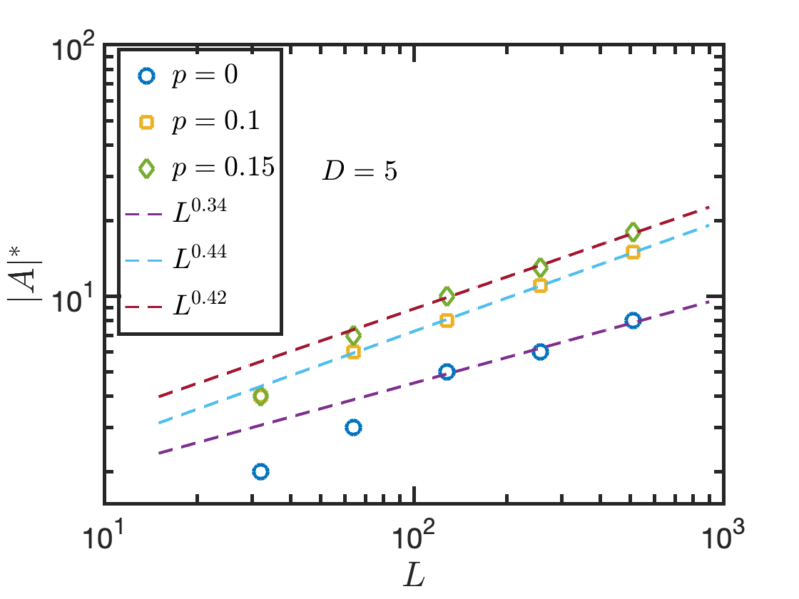
The resilience of the entanglement entropy against measurement in the volume-law phase suggests that the system can be viewed as a dynamically generated quantum error correcting code (QECC) Li and Fisher 2021; Fan et al. 2021. Specifically, the amount of entanglement entropy can be associated with the number of logical qubits encoded, which decreases to zero as one approaches the transition point. An important characterization of a QECC is the (contiguous) code distance, defined as the minimal length of a logical operator acting (in a contiguous region) within the code space. As it turns out, the scaling of the contiguous code distance can also be calculated with the domain wall picture, as a length scale where the dominating domain wall configuration contributing to changes Li and Fisher 2021. This code distance may be conveniently extracted from a non-monotonic behavior of the subsystem entanglement entropy against in the volume-law phase, starting from a maximally mixed initial state.
In RSTNs on a cylinder, the top (or bottom) edge is naturally in a mixed state, and we indeed observe a similar non-monotonic behavior in the subsystem entanglement entropy in the volume-law phase, as shown in Fig. 19(a). The maximum of the entanglement entropy at corresponds to the point beyond which the mutual information between and the bottom edge is zero: , hence measurement in cannot decrease the entanglement entropy Li and Fisher 2021. Therefore, can be identified as the contiguous code distance in our system. In Fig. 19(b), we plot the scaling of with the total system size . Similarly to Ref. Li et al. 2021, the exponents we found are slightly larger than the KPZ prediction , possibly due to the limited system sizes as well as the strong sample-to-sample fluctuations that prevent us from determining accurately. We expect that the code distance should also scale as for sufficiently large .
VI Discussions and outlook
To summarize, we study two types of entanglement phase transitions in RSTNs. When tuning the bond dimension alone, we observe an area law scaling of the boundary entanglement entropy at , and a volume law scaling at prime . This is thus suggestive of a phase transition at between and , provided the tensor network model can be appropriately generalized to non-integer bond dimension .
We observe a second class of phase transitions driven by randomly breaking bonds in the bulk of the RSTN with probability , effectively putting the RSTN on a random lattice. Here, for all prime , we see a continuous phase transition separating a volume law phase of the boundary state at small , and an area law phase at large . The critical points for different values of are apparently described by different CFTs, as summarized in Table 1. With increasing values of , the critical exponents in the corresponding CFT are approaching their counterparts in critical first-passage percolation, suggesting that the critical point is becoming increasingly “percolation like”.
The last point suggests that a “minimal cut” picture is at work as . For example, the entanglement entropy of a single boundary region should differ from the weight of the minimal cut (i.e. the minimal number of bonds a “domain wall” must break, see Fig. 1) by at most an constant:
| (55) |
This relation would reproduce the value of at large (Table 1). Moreover, the entanglement between two disjoint regions, as quantified by the mutual information and the mutual negativity, should also agree with those defined by minimal cuts Skinner et al. 2019; Sang et al. 2020, and are supported by the values of , , and at the large critical points (Table 1).
As we have mentioned earlier in this paper, it is known in RTNs Hayden et al. 2016 and in RSTNs Nezami and Walter 2020 that Eq. (55) holds exactly as if we keep finite. According to Ref. Nezami and Walter 2020, Eq. (55) holds provided that scales as (at least) , such that the deviation from is small. In this work, while we vary to take various prime values that are possibly large in themselves, they are nevertheless small compared to , thus not within the regime where Eq. (55) can be demonstrated analytically as in Ref. Nezami and Walter 2020. For this reason, we are inclined to interpret our results at larger as reliable estimates of operator dimensions in the underlying “percolation like” CFT in the thermodynamic limit , rather than artifacts due to finite system sizes. Thus, a separate justification (or at least a significant improvement of the previous bound Nezami and Walter 2020) is needed for the emergence of these percolation like CFTs observed in this work.
Recently in Ref. Zabalo et al. 2021, the authors pointed out that for monitored random stabilizer circuits (and RSTNs) with where is a prime number, the underlying statistical mechanics models have different symmetries for different values of (see Ref. Li et al. for details). This explains the series of universality classes we observe at different values of . It would be interesting to use these results Zabalo et al. 2021 to explain the percolation like exponents at large .
For completeness, we also briefly summarize the critical properties of monitored random stabilizer circuits for various values of prime , for which detailed results will be reported elsewhere Li et al.. Similarly to RSTNs, we find a series of distinct critical points for each value of (since random circuits will always generate volume-law entangled states for any ), and most of the critical exponents are also approaching critical first-passage percolation with increasing . However, this series of critical points appears to be distinct from those in the RSTN. Understanding their difference is left for future work Li et al..
We have also considered several variations of the RSTN. Upon replacing all the forced measurements – responsible for implementing tensor contraction and bond breaking – with projective measurements (see Appendix D for a detailed description), we find almost identical phase diagrams and critical exponents (data not displayed). Reducing the randomness in the RSTN does not seem to alter the critical exponents significantly (see Sec. IV.7), although the location of may change and the critical point may not be easily accessible. These results suggest the robustness of the critical point against these perturbations.
There are several interesting applications and extensions of the present work which we briefly mention.
Firstly, the area law scaling of entanglement entropy observed on the square lattice at is not universal. In principle, one could construct RSTNs on lattices or graphs with a larger coordination number, so that the RSTNs can host a volume law entangled state. In this case, upon breaking bonds in the bulk, one could drive an entanglement transition. It would then be interesting to explore the critical exponents of these transitions.
Secondly, one could introduce physical qudits in the bulk which correspond to dangling legs of the bulk tensors. In this setup, the entanglement entropy for the boundary qudits may be modified. One could then investigate the bulk-boundary correspondonce and the error correction properties of these RSTNs Hayden et al. 2016; Pastawski et al. 2015; Almheiri et al. 2015; Mintun et al. 2015.
Thirdly, it may be interesting to move away from the fully random RSTN and consider instead those with a restricted class of local tensors, e.g. less entangled tensors, tensors with a global symmetry, and “isometric” tensors for any bipartition of the legs Pastawski et al. 2015. Previously in the context of hybrid circuits, these ideas have lead to a plethora of “measurement-protected quantum phases” Lavasani et al. 2021; Sang and Hsieh 2021; Ippoliti et al. 2021a; Chen et al. 2020; Alberton et al. 2021; Ippoliti and Khemani 2021; Bao et al. 2021; Buchhold et al. 2021; Lu and Grover 2021; Ippoliti et al. 2021b.
Lastly, one may be able to construct tensor network states using tensors that encode the Boltzmann weights of a classical statistical mechanics model Levin and Nave 2007. It would be interesting to explore the implication of a phase transition of the underlying statistical mechanics model on the entanglement properties of the boundary state.
Acknowledgments
We acknowledge useful discussions with Tianci Zhou, Andreas Ludwig, and Romain Vasseur. Z.-C.Y. acknowledges financial support from NSF PFCQC program and DoE ASCR Accelerated Research in Quantum Computing program (award No. DE-SC0020312). This work was supported by the Heising-Simons Foundation (Y.L. and M.P.A.F.), and by the Simons Collaboration on Ultra-Quantum Matter which is a grant from the Simons Foundation (651440, M.P.A.F.). We thank the Aspen Center for Physics where part of this work was carried out, which is supported by National Science Foundation grant PHY-1607611 (M.P.A.F. and X.C.). The numerical calculations were performed on the Boston University Shared Computing Cluster, which is administered by Boston University Research Computing Services.
References
- D’Alessio et al. (2016) L. D’Alessio, Y. Kafri, A. Polkovnikov, and M. Rigol, “From quantum chaos and eigenstate thermalization to statistical mechanics and thermodynamics,” Advances in Physics 65, 239–362 (2016), arXiv:1509.06411 [cond-mat.stat-mech] .
- Deutsch (1991) J. M. Deutsch, “Quantum statistical mechanics in a closed system,” Phys. Rev. A 43, 2046–2049 (1991).
- Srednicki (1994) M. Srednicki, “Chaos and quantum thermalization,” Phys. Rev. E 50, 888–901 (1994).
- Page (1993) D. N. Page, “Average entropy of a subsystem,” Phys. Rev. Lett. 71, 1291–1294 (1993).
- Hastings (2007) M. B. Hastings, “An area law for one-dimensional quantum systems,” Journal of Statistical Mechanics: Theory and Experiment 2007, 08024 (2007), arXiv:0705.2024 [quant-ph] .
- Eisert et al. (2010) J. Eisert, M. Cramer, and M. B. Plenio, “Colloquium: Area laws for the entanglement entropy,” Rev. Mod. Phys. 82, 277–306 (2010).
- Oganesyan and Huse (2007) V. Oganesyan and D. A. Huse, “Localization of interacting fermions at high temperature,” Phys. Rev. B 75, 155111 (2007).
- Pal and Huse (2010) A. Pal and D. A. Huse, “Many-body localization phase transition,” Phys. Rev. B 82, 174411 (2010).
- Nandkishore and Huse (2015) R. Nandkishore and D. A. Huse, “Many-Body Localization and Thermalization in Quantum Statistical Mechanics,” Annual Review of Condensed Matter Physics 6, 15–38 (2015), arXiv:1404.0686 [cond-mat.stat-mech] .
- Chan et al. (2019) A. Chan, R. M. Nandkishore, M. Pretko, and G. Smith, “Unitary-projective entanglement dynamics,” Phys. Rev. B 99, 224307 (2019).
- Skinner et al. (2019) B. Skinner, J. Ruhman, and A. Nahum, “Measurement-induced phase transitions in the dynamics of entanglement,” Phys. Rev. X 9, 031009 (2019).
- Li et al. (2018) Y. Li, X. Chen, and M. P. A. Fisher, “Quantum zeno effect and the many-body entanglement transition,” Phys. Rev. B 98, 205136 (2018).
- Li et al. (2019) Y. Li, X. Chen, and M. P. A. Fisher, “Measurement-driven entanglement transition in hybrid quantum circuits,” Phys. Rev. B 100, 134306 (2019).
- Li et al. (2020) Y. Li, X. Chen, A. W. W. Ludwig, and M. P. A. Fisher, “Conformal invariance and quantum non-locality in hybrid quantum circuits,” arXiv e-prints , arXiv:2003.12721 (2020), arXiv:2003.12721 [quant-ph] .
- Bao et al. (2020) Y. Bao, S. Choi, and E. Altman, “Theory of the phase transition in random unitary circuits with measurements,” Phys. Rev. B 101, 104301 (2020).
- Jian et al. (2020) C.-M. Jian, Y.-Z. You, R. Vasseur, and A. W. W. Ludwig, “Measurement-induced criticality in random quantum circuits,” Phys. Rev. B 101, 104302 (2020).
- Choi et al. (2020) S. Choi, Y. Bao, X.-L. Qi, and E. Altman, “Quantum error correction in scrambling dynamics and measurement-induced phase transition,” Phys. Rev. Lett. 125, 030505 (2020).
- Gullans and Huse (2020) M. J. Gullans and D. A. Huse, “Dynamical Purification Phase Transition Induced by Quantum Measurements,” Physical Review X 10, 041020 (2020), arXiv:1905.05195 [quant-ph] .
- Fan et al. (2021) R. Fan, S. Vijay, A. Vishwanath, and Y.-Z. You, “Self-organized error correction in random unitary circuits with measurement,” Phys. Rev. B 103, 174309 (2021).
- Li and Fisher (2021) Y. Li and M. P. A. Fisher, “Statistical mechanics of quantum error correcting codes,” Phys. Rev. B 103, 104306 (2021).
- Fidkowski et al. (2021) L. Fidkowski, J. Haah, and M. B. Hastings, “How Dynamical Quantum Memories Forget,” Quantum 5, 382 (2021), arXiv:2008.10611 [quant-ph] .
- Gullans et al. (2020) M. J. Gullans, S. Krastanov, D. A. Huse, L. Jiang, and S. T. Flammia, “Quantum coding with low-depth random circuits,” arXiv e-prints , arXiv:2010.09775 (2020), arXiv:2010.09775 [quant-ph] .
- Zabalo et al. (2020) A. Zabalo, M. J. Gullans, J. H. Wilson, S. Gopalakrishnan, D. A. Huse, and J. H. Pixley, “Critical properties of the measurement-induced transition in random quantum circuits,” Phys. Rev. B 101, 060301 (2020), arXiv:1911.00008 [cond-mat.dis-nn] .
- Zabalo et al. (2021) A. Zabalo, M. J. Gullans, J. H. Wilson, R. Vasseur, A. W. W. Ludwig, S. Gopalakrishnan, D. A. Huse, and J. H. Pixley, “Operator scaling dimensions and multifractality at measurement-induced transitions,” arXiv e-prints , arXiv:2107.03393 (2021), arXiv:2107.03393 [cond-mat.dis-nn] .
- Hayden et al. (2016) P. Hayden, S. Nezami, X.-L. Qi, N. Thomas, M. Walter, and Z. Yang, “Holographic duality from random tensor networks,” Journal of High Energy Physics 2016, 9 (2016), arXiv:1601.01694 [hep-th] .
- Vasseur et al. (2019) R. Vasseur, A. C. Potter, Y.-Z. You, and A. W. W. Ludwig, “Entanglement transitions from holographic random tensor networks,” Phys. Rev. B 100, 134203 (2019).
- Lopez-Piqueres et al. (2020) J. Lopez-Piqueres, B. Ware, and R. Vasseur, “Mean-field entanglement transitions in random tree tensor networks,” Physical Review B 102 (2020), 10.1103/physrevb.102.064202.
- Perez-Garcia et al. (2006) D. Perez-Garcia, F. Verstraete, M. M. Wolf, and J. I. Cirac, “Matrix Product State Representations,” arXiv e-prints , quant-ph/0608197 (2006), arXiv:quant-ph/0608197 [quant-ph] .
- Schollwöck (2011) U. Schollwöck, “The density-matrix renormalization group in the age of matrix product states,” Annals of Physics 326, 96–192 (2011), arXiv:1008.3477 [cond-mat.str-el] .
- Verstraete et al. (2008) F. Verstraete, V. Murg, and J. I. Cirac, “Matrix product states, projected entangled pair states, and variational renormalization group methods for quantum spin systems,” Advances in Physics 57, 143–224 (2008), arXiv:0907.2796 [quant-ph] .
- Orús (2014) R. Orús, “A practical introduction to tensor networks: Matrix product states and projected entangled pair states,” Annals of Physics 349, 117–158 (2014), arXiv:1306.2164 [cond-mat.str-el] .
- Vidal (2008) G. Vidal, “Class of quantum many-body states that can be efficiently simulated,” Phys. Rev. Lett. 101, 110501 (2008).
- Jahn et al. (2018) A. Jahn, M. Gluza, F. Pastawski, and J. Eisert, “Holography and criticality in matchgate tensor networks,” (2018), arXiv:1711.03109 [quant-ph] .
- Ryu and Takayanagi (2006) S. Ryu and T. Takayanagi, “Holographic derivation of entanglement entropy from the anti–de sitter space/conformal field theory correspondence,” Phys. Rev. Lett. 96, 181602 (2006).
- Swingle (2012) B. Swingle, “Entanglement renormalization and holography,” Phys. Rev. D 86, 065007 (2012).
- Jiang and Yao (2016) J. Jiang and C.-L. Yao, “Critical first-passage percolation starting on the boundary,” arXiv e-prints , arXiv:1612.01803 (2016), arXiv:1612.01803 [math.PR] .
- Sang et al. (2020) S. Sang, Y. Li, T. Zhou, X. Chen, T. H. Hsieh, and M. P. A. Fisher, “Entanglement Negativity at Measurement-Induced Criticality,” arXiv e-prints , arXiv:2012.00031 (2020), arXiv:2012.00031 [cond-mat.stat-mech] .
- Gottesman (1997) D. Gottesman, Stabilizer codes and quantum error correction, Ph.D. thesis, California Institute of Technology (1997), arXiv:quant-ph/9705052 [quant-ph] .
- Gottesman (1998) D. Gottesman, “The Heisenberg Representation of Quantum Computers,” arXiv e-prints , quant-ph/9807006 (1998), arXiv:quant-ph/9807006 [quant-ph] .
- Aaronson and Gottesman (2004) S. Aaronson and D. Gottesman, “Improved simulation of stabilizer circuits,” Physical Review A 70, 052328 (2004), arXiv:quant-ph/0406196 [quant-ph] .
- Nezami and Walter (2020) S. Nezami and M. Walter, “Multipartite entanglement in stabilizer tensor networks,” Phys. Rev. Lett. 125, 241602 (2020).
- Gottesman (1999) D. Gottesman, “Fault-Tolerant Quantum Computation with Higher-Dimensional Systems,” Chaos Solitons and Fractals 10, 1749–1758 (1999), arXiv:quant-ph/9802007 [quant-ph] .
- Huse and Henley (1985) D. A. Huse and C. L. Henley, “Pinning and roughening of domain walls in ising systems due to random impurities,” Phys. Rev. Lett. 54, 2708–2711 (1985).
- Kardar (1985) M. Kardar, “Roughening by impurities at finite temperatures,” Phys. Rev. Lett. 55, 2923–2923 (1985).
- Huse et al. (1985) D. A. Huse, C. L. Henley, and D. S. Fisher, “Huse, henley, and fisher respond,” Phys. Rev. Lett. 55, 2924–2924 (1985).
- Li et al. (2021) Y. Li, S. Vijay, and M. P. A. Fisher, “Entanglement Domain Walls in Monitored Quantum Circuits and the Directed Polymer in a Random Environment,” arXiv e-prints , arXiv:2105.13352 (2021), arXiv:2105.13352 [cond-mat.stat-mech] .
- Kardar et al. (1986) M. Kardar, G. Parisi, and Y.-C. Zhang, “Dynamic scaling of growing interfaces,” Phys. Rev. Lett. 56, 889–892 (1986).
- Jian et al. (2020) C.-M. Jian, B. Bauer, A. Keselman, and A. W. W. Ludwig, “Criticality and entanglement in non-unitary quantum circuits and tensor networks of non-interacting fermions,” arXiv e-prints , arXiv:2012.04666 (2020), arXiv:2012.04666 [cond-mat.stat-mech] .
- Nahum et al. (2020) A. Nahum, S. Roy, B. Skinner, and J. Ruhman, “Measurement and entanglement phase transitions in all-to-all quantum circuits, on quantum trees, and in Landau-Ginsburg theory,” arXiv e-prints , arXiv:2009.11311 (2020), arXiv:2009.11311 [cond-mat.stat-mech] .
- Kesten (1986) H. Kesten, “Aspects of first passage percolation,” in École d’été de probabilités de Saint Flour XIV-1984 (Springer, 1986) pp. 125–264.
- Chayes et al. (1986) J. T. Chayes, L. Chayes, and R. Durrett, “Critical behavior of the two-dimensional first passage time,” Journal of Statistical Physics 45, 933–951 (1986).
- Cardy (1984) J. L. Cardy, “Conformal invariance and surface critical behavior,” Nuclear Physics B 240, 514–532 (1984).
- Cardy (2004) J. Cardy, “Boundary Conformal Field Theory,” arXiv e-prints , hep-th/0411189 (2004), arXiv:hep-th/0411189 [hep-th] .
- Driscoll and Trefethen (2002) T. A. Driscoll and L. N. Trefethen, Schwarz-christoffel mapping, Vol. 8 (Cambridge University Press, 2002).
- Nahum and Skinner (2020) A. Nahum and B. Skinner, “Entanglement and dynamics of diffusion-annihilation processes with Majorana defects,” Physical Review Research 2, 023288 (2020), arXiv:1911.11169 [cond-mat.stat-mech] .
- Belavin et al. (1984) A. A. Belavin, A. M. Polyakov, and A. B. Zamolodchikov, “Infinite conformal symmetry in two-dimensional quantum field theory,” Nuclear Physics B 241, 333–380 (1984).
- Vidal and Werner (2002) G. Vidal and R. F. Werner, “Computable measure of entanglement,” Phys. Rev. A 65, 032314 (2002).
- Shi et al. (2020) B. Shi, X. Dai, and Y.-M. Lu, “Entanglement negativity at the critical point of measurement-driven transition,” arXiv e-prints , arXiv:2012.00040 (2020), arXiv:2012.00040 [cond-mat.stat-mech] .
- Gullans and Huse (2019) M. J. Gullans and D. A. Huse, “Scalable probes of measurement-induced criticality,” arXiv e-prints , arXiv:1910.00020 (2019), arXiv:1910.00020 [cond-mat.stat-mech] .
- Cardy (1992) J. L. Cardy, “Critical percolation in finite geometries,” Journal of Physics A Mathematical General 25, L201–L206 (1992), arXiv:hep-th/9111026 [hep-th] .
- Lang and Büchler (2020) N. Lang and H. P. Büchler, “Entanglement transition in the projective transverse field Ising model,” Phys. Rev. B 102, 094204 (2020), arXiv:2006.09748 [cond-mat.dis-nn] .
- Kardar and Zhang (1987) M. Kardar and Y.-C. Zhang, “Scaling of directed polymers in random media,” Phys. Rev. Lett. 58, 2087–2090 (1987).
- (63) Y. Li, R. Vasseur, M. P. A. Fisher, and A. W. W. Ludwig, Unpublished.
- Pastawski et al. (2015) F. Pastawski, B. Yoshida, D. Harlow, and J. Preskill, “Holographic quantum error-correcting codes: toy models for the bulk/boundary correspondence,” Journal of High Energy Physics 2015, 149 (2015), arXiv:1503.06237 [hep-th] .
- Almheiri et al. (2015) A. Almheiri, X. Dong, and D. Harlow, “Bulk locality and quantum error correction in AdS/CFT,” Journal of High Energy Physics 2015, 163 (2015), arXiv:1411.7041 [hep-th] .
- Mintun et al. (2015) E. Mintun, J. Polchinski, and V. Rosenhaus, “Bulk-Boundary Duality, Gauge Invariance, and Quantum Error Corrections,” Phys. Rev. Lett. 115, 151601 (2015), arXiv:1501.06577 [hep-th] .
- Lavasani et al. (2021) A. Lavasani, Y. Alavirad, and M. Barkeshli, “Measurement-induced topological entanglement transitions in symmetric random quantum circuits,” Nature Physics 17, 342–347 (2021), arXiv:2004.07243 [quant-ph] .
- Sang and Hsieh (2021) S. Sang and T. H. Hsieh, “Measurement-protected quantum phases,” Physical Review Research 3, 023200 (2021), arXiv:2004.09509 [cond-mat.stat-mech] .
- Ippoliti et al. (2021a) M. Ippoliti, M. J. Gullans, S. Gopalakrishnan, D. A. Huse, and V. Khemani, “Entanglement Phase Transitions in Measurement-Only Dynamics,” Physical Review X 11, 011030 (2021a), arXiv:2004.09560 [quant-ph] .
- Chen et al. (2020) X. Chen, Y. Li, M. P. A. Fisher, and A. Lucas, “Emergent conformal symmetry in non-unitary random dynamics of free fermions,” arXiv e-prints , arXiv:2004.09577 (2020), arXiv:2004.09577 [quant-ph] .
- Alberton et al. (2021) O. Alberton, M. Buchhold, and S. Diehl, “Entanglement Transition in a Monitored Free-Fermion Chain: From Extended Criticality to Area Law,” Phys. Rev. Lett. 126, 170602 (2021), arXiv:2005.09722 [cond-mat.stat-mech] .
- Ippoliti and Khemani (2021) M. Ippoliti and V. Khemani, “Postselection-Free Entanglement Dynamics via Spacetime Duality,” Phys. Rev. Lett. 126, 060501 (2021), arXiv:2010.15840 [cond-mat.dis-nn] .
- Bao et al. (2021) Y. Bao, S. Choi, and E. Altman, “Symmetry enriched phases of quantum circuits,” arXiv e-prints , arXiv:2102.09164 (2021), arXiv:2102.09164 [cond-mat.stat-mech] .
- Buchhold et al. (2021) M. Buchhold, Y. Minoguchi, A. Altland, and S. Diehl, “Effective Theory for the Measurement-Induced Phase Transition of Dirac Fermions,” arXiv e-prints , arXiv:2102.08381 (2021), arXiv:2102.08381 [cond-mat.stat-mech] .
- Lu and Grover (2021) T.-C. Lu and T. Grover, “Entanglement transitions via space-time rotation of quantum circuits,” arXiv e-prints , arXiv:2103.06356 (2021), arXiv:2103.06356 [quant-ph] .
- Ippoliti et al. (2021b) M. Ippoliti, T. Rakovszky, and V. Khemani, “Fractal, logarithmic and volume-law entangled non-thermal steady states via spacetime duality,” arXiv e-prints , arXiv:2103.06873 (2021b), arXiv:2103.06873 [quant-ph] .
- Levin and Nave (2007) M. Levin and C. P. Nave, “Tensor Renormalization Group Approach to Two-Dimensional Classical Lattice Models,” Phys. Rev. Lett. 99, 120601 (2007), arXiv:cond-mat/0611687 [cond-mat.stat-mech] .
Appendix A Numerical results for the mutual information on a cylinder for and


We show additional numerical results for the mutual information of cylindrical random tensor networks with and in Fig. 20. We again see a peak at some critical measurement rate in both cases, indicating the existence of an entanglement transition. Furthermore, the critical value increases towards as increases.
Appendix B The Schwarz-Christoffel mapping from a finite rectangle to the lower half plane

In this section, we explain in detail the Schwarz-Christoffel mapping that conformally maps a finite rectangle to the lower half plane Li et al. 2020. The Schwarz-Christoffel mapping proceeds in two steps, as illustrated in Fig. 21: (1) mapping to a “canonical rectangle” via a scale transformation; (2) mapping from the canonical rectangle to the lower half plane. The first step transforms the original rectangle of size to one of size , where is the complete elliptic integral of the first kind. The parameter can be solved numerically by requiring that the aspect ratio remains unchanged:
| (56) |
Notice that since the tensor network is isotropic along the and directions microscopically, the aspect ratio of the system when viewed as a CFT is exactly given by . Then, one can go from the original complex -plane to the -plane by the rescaling:
| (57) |
The second step is achieved via the Jacobi sn function, which is the inverse of the elliptic integral :
| (58) |
This maps the boundary of the rectangle to the real axis. In Fig. 21 we show the image of the four corners of the rectangle under this mapping.
Under a conformal transformation, correlation functions of primary fields in a CFT transform as Belavin et al. 1984:
| (59) |
where is the scaling dimension of the field . Applying the above transformation to the example of Eq. (24):
This leads to Eq. (25) in the main text, where we define , so as to show explicitly the factor of when is varied, and is finite as becomes large. In particular, since , we obtain
| (61) |
where and are the other two Jacobi elliptic functions.
Appendix C Proof of the negativity formula Eq. (37)
We now prove Eq. (37) in the main text, which provides a simple method for computing the mutual negativity for stabilizer states. The proof follows directly from the method in Ref. Sang et al. 2020. Let us first define the stabilizer subgroup supported on subsystem and its generators:
| (62) |
where . The density matrix on can be represented in terms of the group elements of :
| (63) |
The mutual negativity (33) is related to the partial transpose of on subsystem :
| (64) |
where
| (65) |
In terms of the Pauli strings, takes the form:
| (66) |
where we have ignored an unimportant global phase factor. Using properties of the Pauli matrices under transpose , , it is straightforward to show that
| (67) |
where , and we have defined shorthand notations and . Similarly, we define . Thus, we have an explicit form of under partial transpose:
| (68) |
Notice that in the special case , the above relations become , , so that , and depending on the parity of the operators appearing in . This is the case considered in Ref. Sang et al. 2020.
Next, we define a function , such that
| (69) |
We will also need the commutation matrix defined in Eq. (35). Since encodes the commutation relations between each pair of generators of , the phase between an arbitrary pair of can be calculated using . Let us write in terms of the generators of :
| (70) |
where the expansion coefficients can be encoded in a vector for prime . Similarly, can also be represented as a vector . Therefore, we have
| (71) |
Below, we shall use the vector to denote the Pauli string of , and for the expansion of in terms of the generators .
With all the ingredients above, we shall now derive a key result for the proof of Eq. (37):
| (72) |
We start by computing :
| (73) | |||||
The calculations above need some explanations. In the fourth line, we have used the following relation:
| (74) |
where and denote the Pauli strings in and , respectively. In the fifth line, we have used the relation:
| (75) |
which can be verified via a direct calculation. Notice that in the special case , this reduces to the “cocycle condition” discussed in Ref. Sang et al. 2020. Using the result of Eq. (73), we can now proceed to compute :
| (76) | |||||
This immediately implies that
| (77) |
Finally, using the last expression above, we are ready to prove Eq. (37):
| (78) | |||||
This is exactly Eq. (37).
Appendix D Forced measurements, projective measurements, and sampling algorithms
In this Appendix, we explain the numerical method for sampling the random tensor networks, and explain two possible probability distributions that we can assign to these random samples. As we will see, they effectively define two models we considered in the main text, with “forced meaurements” and “projective measurements”, repsectively.
D.1 Forced measurements for tensor contraction
The algorithm for sampling a particular instance of the random stabilizer tensor network with forced measurements is as follows.
- 1.
We start with the following computational basis state
(79) Here, we have taken .
- 2.
Next, for each site we sample a random Clifford unitary from the uniform probability distribution on the 4-qudit Clifford group (denoted ); the result is denoted .
The unitaries define a tensor on each site, namely
(80) or equivalently
(81) We then have the following state,
(82) Here is an element of .
- 3.
Finally, we project pairs of qudits on each bulk bond of the network to a fixed Bell state , effectively contracting the indices of the tensor network. After that we trace out qudits in the bulk. These operations can be summarized as follows,
(83) where
(84) That is, the projection operator is realized by “forcing” or “post-selecting” the trajectory where all measurement outcomes (that is, of all and operators on all bulk edges) equal to .
With the bulk qudits traced out, is a pure state on the boundary qudits of the tensor network.
As defined, is not necessarily normalized. Its trace is equal to the probability that the aforementioned “all ” trajectory occurs, in the ensemble of all possible measurement trajectories. In numerics, we can formally perform the projection and subsequently normalize the state, without worrying about physical meanings of the post-selection, except when , which means that the contraction of indices gives a zero state, and we must reject the sample given by . This may be numerically unfavorable, for the construction of a state can be quite time consuming.
When , we denote the normalized density matrix as
| (85) |
Thus, we have now the following ensemble of normalized boundary states, each occuring with the same probability.
| (86) |
where we defined the following subset of
| (87) |
Note that while different elements of can in principle give rise to the same , we still treat them differently, so that .
We can now discuss what probability distribution (or “measure”) we want to assign on . Here, we choose to assign each element of with equal probability . Formally, it means that the ensemble average of an observable should read
| (88) |
The superscript “f” means “forced measurements”, to be distinguished from the case with projective measurements, below.
To numerically estimate , we may run the sampling algorithm times (each run will give us an instance of unitary ), and average the results against the runs for which the resultant state does not vanish. Formally, this reads
| (89) |
for which we expect
| (90) |
D.2 Projective measurements
Instead of forcing the and measurements on the edges and focusing on a single trajectory so that we manage to contract the indices of an abstract tensor network, in this subsection we instead view the measurements as “physical”, and consider the ensemble of all possible measurement trajectories weighted by their respective Born probabilities, without rejecting any of them. This way, we can define a different ensemble of RSTN.
Formally, we now have the following ensemble of normalized boundary states,
| (91) |
Here, the state is labelled by not only the unitary , but also all admissible trajectories (i.e. those with nonzero probability) of the measurements, , where
The weight we assign to states in is the Born probability, . The ensemble average of an observable is thus
| (92) |
From now on, we focus on entanglement properties of the boundary stabilizer states (and can be the entropy, mutual information between subregions, entanglement negativities, as we considered in the main text), for which all trajectories lead to the same value of . The result really only depends on the unitary , which we denote as , where can be chosen to be any admissible trajectory. Thus,
| (93) |
where we used the conservation of probability,
| (94) |
We emphasize that the simplification in Eq. (D.2) only occurs for entanglement properties of stabilizer states. In contrast, Eq. (88) is completely general, and remains correct for generic (non-stabilizer states) and any observable .
To numerically estimate the ensemble avaraged entanglement properties , we may run the sampling algorithm times. In each run, we can take any trajectory , and calculate for the resultant state . In practice, in running the stabilizer simulation, one can simply choose to not record the measurement outcomes at all; the resultant state is guaranteed to be on an admissible trajectory.44 4 The same method can also be applied in the simulation of random Clifford circuits where the results are weighted by the Born probability. Thus, we do not need to reject any of the runs. The estimate is thus
| (95) |
for which we also expect
| (96) |
D.3 Relating the two ensembles
We have defined and , and defined sampling methods for estimating them, in Eqs. (89, 95), respectively. As we explained above, in estimating with Eq. (89), some samples must be rejected. Here, we describe a single sampling method for entanglement properties , where both and can be estimated, without the need of rejectign any sample.
We start by comparing the definitions of [Eq. (88)] and [Eq. (D.2)]. It will be convenient now to explicitly include the trajectory information in Eq. (88), replacing
| (97) |
where denotes the trajectory where all measurement results are (as we needed for contracting the indices)
| (98) |
With this replacement, Eq. (88) now reads
| (99) |
For in Eq. (D.2), for all , we may also choose , by definition. Thus,
| (100) |
For , must not be equal to , but otherwise arbitrary as long as .
It is a property of stabilizer states that must either be or of the form , where is an integer between and , which is equal to the number measurements whose results are random, and only depends on . For example, when on one trajectory , all measurements are random; and in fact we have the same trace for all trajectories,
| (101) |
In general, when , there are trajectories, and all of them will have the same trace.
For the mutually commuting operators that has been measured , we introduce for each of them a “destabilizer”, , which are single qudit unitaries that satisfy the following commutation relations
| (102) | ||||
| (103) |
We now construct a mapping from to as follows.
- 1.
If , we simply take .
- 2.
If , we must have that , and exactly measurements have deterministic results. Among these , at least one of the deterministic results is not equal to .
In this case, we define
(104) That is, and are related by local Clifford unitaries that do not change the entanglement properties. Morever, measurements of that are random for will remain random for , and those that are deterministic remain deterministic for . The powers are uniquely fixed by the condition that the deterministic results for are all . Thus, .
Clearly, the mapping assign a unique image to each , thus well defined. Thus, we may partition according to the image under ,
| (105) |
where by definition and are disjoint sets for . Moreover, for all , we have.
| (106) |
With these, we have
| (107) | ||||
| (108) |
and
| (109) |
We used again the fact that the mapping does not affect the value of .
These results allow us to use the estimates for estimating . Again, we sample unitaries , in the same fashion that led to Eq. (95). Then, we calculate the following modified weighted estimate
| (110) |
Both the numerator and the denominator takes the form of a . As we take ,
| (111) |
Thus, by assigning the weight to each sample, and compute the weighted average, we obtain an estimate of .
D.4 Sampling from the forced measurement ensemble with local rejections
Directly computing in the numerics leads to a problem of “undersampling”, i.e. having an insufficient number of samples. The denominator of Eq. (110) can be thought of as the effective number of samples, and is observed to grow slowly with . Recall that is the total number of bond contraction measurements whose outcomes are deterministic, thus its typical value grows with the system size, severely suppresing the weight of the samples.
In practice, instead of assigning a weight to the entire tensor network at the end, we choose to probablistically reject samples at a local level, so that each tensor network occur with a probability proportional to , and no adjustments of the weights need to be made at the end. The detailed procedure is as follows.
- 1.
We generate the local tensors at each location one by one, in the order of increasing and . Recall that the local tensor is generated by sampling a 4-qudit Clifford unitary.
- 2.
Once the local tensor at is generated, we attempt to contract its bonds with and , so that it becomes a part of the entire tensor network.
- 3.
The contractions are realized by performing two measurements (of and of ) that are forced to have results . In the case of both measurements have random outcomes, we accept the local tensor. If exactly one of the measurements have random outcomes, we accept the local tensor with probability , by flipping a biased coin. If both measurements have deterministic outcomes, we accept the local tensor with probability .
- 4.
If a local tensor is not accepted, we say it is rejected, in which case we regenerate the local tensor by sampling a new 4-qudit Clifford unitary, and attempt the two contraction measurements again.
To see that this algorithm is correct, we compare it with the sampling procedure in Eq. (110).
- 1.
Instead of assigning weights to different samples as in (see Eq. (110)), here we use probabilistic acceptance, which is completely equivalent. We can imagine generating each sample as in Eq. (110), but accept with probability . Although highly inefficient, in the limit the unweighted average will converge to and .
- 2.
Following the previous point, instead of deciding whether or not to accept the entire tensor network at the end, we choose to perform the probabilistic acceptance/rejection at a local level, which only depends on local information. In other words, we can perform the rejections early, so we do not have to contract all the tensors before we find out this sample needs to be rejected.
- 3.
Moreover, since each sample has a finite probability to be accepted, we never run into a case where it is impossible to find a acceptable local tensor. Thus, we are guaranteed to get a sample, of weight 1, for each run of the algorithm. This property is again special to the stabilizer tensor networks.
To generate samples with this algorithm, the running time is proportional to . The local rejections lead to a mere constant multiple of overhead.
Although the algorithm above is described only for the forced measurements involved in contraction of bonds, it is straightforward to modify it so that forced measurements responsible for breaking bonds can also be implemented.