Universal spin mixing oscillations in a strongly interacting one-dimensional Fermi gas
Abstract
We study the spin-mixing dynamics of a one-dimensional strongly repulsive Fermi gas under harmonic confinement. By employing a mapping onto an inhomogeneous isotropic Heisenberg model and the symmetries under particle exchange, we follow the dynamics till very long times. Starting from an initial spin-separated state, we observe superdiffusion, spin-dipolar large amplitude oscillations and thermalization. We report a universal scaling of the oscillations with particle number . Our study puts forward one-dimensional correlated fermions as a new system to observe the emergence of non-equilibrium universal features.
Elucidating the dynamics of interacting Fermi gases is important for understanding a large variety of physical phenomena, from condensed matter to plasmas and astrophysical objects as neutron stars. The strongly out-of-equilibrium dynamics of interacting quantum systems is currently one of the most challenging open problems.
In this context, the spin dynamics deserves a specific focus. Spin currents can be easily damped by inter-particle collisions Polini and Vignale 2007 and the continuity equation for the spin density includes both orbital current and spin torque contributions Ralph and Stiles 2008. Spin drag is another manifestation of interactions among the spin species, inducing spin-diffusive or non-dissipative dynamics depending on the interaction regimes D’Amico and Vignale 2000; D’Amico and Vignale 2002; Polini and Vignale 2007; Enss and Haussmann 2012; Carlini and Stringari 2021; Valtolina et al. 2017. Ultracold atomic gases provide an ideal platform for exploring in isolated conditions the out-of-equilibrium spin dynamics Volosniev et al. 2015; Barfknecht et al. 2019; Mestyán et al. 2019. In a three dimensional geometry, the oscillatory dynamics of a strongly interacting Fermi gas with initially spatially separated spin components was studied in Sommer et al. 2011. The spin drag, spin diffusivity and spin susceptibility were obtained, and a universal limit for spin diffusivity at low temperature was reported for the unitary Fermi gas.
A relevant question is what happens to the above quantities when reducing the dimensionality of the system to quasi one-dimensional, and what type of universality emerges. One-dimensional (1D) systems display specific features, as the enhancement of quantum fluctuations and correlations and they can be described by a wealth of theoretical and numerical methods Gaudin 1967; Yang 1967; Syrwid et al. 2022; Koutentakis et al. 2019. The quantum dynamics may be strongly affected by the geometrical constraints, as well as by the presence of a large number of conserved quantities, as demonstrated e.g. in the quantum Newton’s cradle experiment Kinoshita et al. 2006.
We address this question by following the dynamics of strongly repulsive fermions subjected to a longitudinal harmonic confinement in a tight waveguide. As in the three-dimensional case of Ref.Sommer et al. 2011, we start from an initially imbalanced state with all spin up on the left and all spin down on the right of the harmonic trap, and we follow the damped oscillations of the magnetization. While the fully quantum dynamics at arbitrary interactions can be followed only at short times with a classical simulator, we focus here on the strongly correlated regime of very large interactions, close to the integrable point at infinite repulsions Harshman et al. 2017; Volosniev et al. 2014; Deuretzbacher et al. 2008a; Decamp et al. 2016; Fang et al. 2011; Murmann et al. 2015; Boll et al. 2016. In this regime, the dynamics of the charge and spin decouple, and the spin dynamics can be followed exactly till very long times by means of a mapping onto the one of an inhomogeneous, isotropic Heisenberg model Sutherland 2004; Franchini 2017 with site-dependent couplings Deuretzbacher et al. 2014; Deuretzbacher et al. 2016.

An overview of the full spin dynamics is provided in Fig. 1, where three main dynamical regimes arise. At short times, we predict the emergence of a superdiffusive behaviour, compatible with Kardar-Parisi-Zhang (KPZ) universality, in striking difference from the diffusive one found in the three-dimensional counterpartSommer et al. 2011. We thus identify 1D correlated fermions as a new system to observe the emergence of non-equilibrium universality, largely explored in homogeneous Heisenberg models Ljubotina et al. 2017; Gobert et al. 2005; Ilievski et al. 2018; De Nardis et al. 2019; Ljubotina et al. 2019; Gopalakrishnan and Vasseur 2019; Dupont and Moore 2020; Bastianello et al. 2022 and experimentally evidenced in quantum magnets and in ultracold atoms on a lattice Bulchandani 2020; Iversen et al. 2020; Wei et al. 2021; Scheie et al. 2021. At intermediate times, we observe large-amplitude spin-dipole oscillations and we obtain the spin drag decay rate. We unveil a scaling in the oscillation frequency, implying a slow-down of the motion and the decrease of the zero-temperature spin drag rate as the particle number grows.
At long times, the oscillations are damped out and the system thermalizes to the diagonal ensemble Rigol et al. 2008. From the analysis of the energy levels distribution we find that the system is weakly non-integrable. The proposed setup allows to explore the conditions for emergence of non-equilibrium universal behaviour in relation to the breaking of its integrability in one dimension.
Model and dynamics
We consider a one-dimensional SU(2) interacting Fermi gas confined in a harmonic trap. The Hamiltonian for such system reads
| (1) |
where is the total number of particles and we take , is the frequency of the harmonic trap and we model the interspecies interaction using a delta potential of strength . Hamiltonian (1) is characterized by the symmetry under exchange of particles having the same spin. For SU(2) fermions, the eigenstates can be classified by the irreducible representations of the permutation group (see eg. Decamp et al. 2016).
We focus on the strongly repulsive limit : in this regime the model is exactly solvable Volosniev et al. 2014 and the wavefunction is given by:
| (2) |
where is the characteristic function of the coordinate sector , are phases depending on the spin ordering of the corresponding coordinate sector and the summation is performed over all the possible permutations of elements. The function is the wavefunction of a -particle non-interacting Fermi gas in the same external potential, i.e. the anti-symmetric product of eigenfunctions of the harmonic oscillator. Remarkably, in the limit the spin and spatial (’charge’) degrees of freedom are decoupled in the wavefunction.
We determine the phases in Eq.(2) to first order in by mapping the Hamiltonian (1) into an effective spin chain:
| (3) |
where is the transposition operator on the chain of sites and is the Fermi energy. The coefficients are site-dependent hopping parameters of the chain, carrying information on the external potential and on the atom-atom interaction of the original fermionic problem sup. The explicit expression reads con:
| (4) |
We classify the basis vectors of the Hilbert space associated to (3) according to the spin ordering on the chain (the so-called snippet basis Deuretzbacher et al. 2008b). For example, for the vector indicates that all the spins are placed in the left half of the chain. Therefore, the dimension of the Hilbert space is . The diagonalization of Eq. (3) allows us to calculate the and thus several observables such as the spin densities . This allows to study the dynamics of the trapped system with an arbitrary initial state.
In this work we follow the fermion dynamics starting from the initially strongly out-of-equilibrium state , as in Ref.Sommer et al. 2011, where the spins up and down are separated in the two opposite sides of the trap. Since the harmonic trap is unchanged, the spatial part of the wavefunction (2) is constant during the motion, hence are constant in time. The time evolution involves only the spin degrees of freedom and can be obtained using the effective spin chain Hamiltonian (3). Recalling that the spin operators are related to the permutation operator by the relation , Hamiltonian (1) can be mapped to the one of an inhomogeneous isotropic Heisenberg model , but in particle space, ie each lattice site is associated to a particle index. The equation of motion for the spin operator for the -th particle reads
| (5) |
where . and is the torque acting on a fixed particle due to the coupling with the neighbouring ones sup. As a result of Eq. (5) we conclude that in our case the spin dynamics is entirely due to spin torque sup.
The experimentally accessible component of such spin vector is , associated to the local magnetization
| (6) |
where is the spatial density of the -th particle in the trap Deuretzbacher et al. 2014; sup, and is the time-evolved spin state, obtained from the diagonalization of by exploiting all its symmetries. The magnetization is experimentally accessible by recording the population imbalance among and fermions, .
Another important observable for the dynamics is the spin current density
| (7) |
where are obtained from the component of Eq. (5), We detail in the following the spin-mixing dynamics in the various relevant time regimes. Systems up to particles have been analyzed using exact diagonalization, while we used truncated Taylor series approximation of the time evolution operator Al-Mohy and Higham 2011 and tDMRG Peotta et al. 2012 to study larger systems.

Short times
The short time dynamics, before the first spin oscillation, is shown in Fig. 2. We show the magnetization as a function of space and time, showing that the initially sharp magnetization interface spreads with time, till it starts feeling the effect of the confining potential. To identify the nature of the magnetization spreading, it is useful to study the time-integrated spin current density as in Ljubotina et al. 2017, , where is defined in Eq.(7) and it is calculated at the center of the trap. We see that the integrated spin current displays a superdiffusive behaviour , with power law exponent . This is compatible with the value predicted for the homogeneous spin chain and clearly not ballistic nor diffusive.Remarkably, low-energy dynamics described by Luttinger liquid predicts ballistic behaviour Polini and Vignale 2007: the deviation from this prediction discloses the marked out-of-equilibrium features of the physical system that are described in an exact way by our model. Using DMRG calculations we have checked that the KPZ region persists for larger numbers of particles (see Fig.2) The deviation at later times from KPZ behaviour is due to onset of the oscillatory dynamics associated to the presence of the external trap. Within the KPZ region, we find that the magnetization profiles collapse onto each other if plotted as a function of , being the KPZ value for the dynamical critical exponent.
Intermediate times
We next focus on the intermediate time regime, when the particles undergo large-amplitude spin-dipole oscillations in the trap. We follow the center of mass oscillations of the magnetization,
| (8) |
The time evolution of is shown in Fig. 3a for various values of the number of particles. We observe damped oscillations tending to a plateau corresponding to zero magnetization. At later times (not shown in the figure), the dynamics undergoes several partial revivals, as expected since we describe a closed quantum system. Quite remarkably, we find that the various curves for different particle numbers collapse one to another if we scale the time axis by a factor with . Using DMRG simulations up to particles sup, we have tested that the scaling is robust at increasing particle numbers. The magnetization oscillations are well approximated by a damped harmonic oscillator (see Fig. 3b). This allows us to obtain the oscillation frequency for the various values. We find that the damping rate doesn’t depend on the number of particles. Combining the two values, we obtain the spin drag rate as D’Amico and Vignale 2000; D’Amico and Vignale 2002; Sommer et al. 2011; spi.
We also perform a spectral analysis of by introducing the spectral function . In Fig. 3c we show and the Fourier transform of the fitted signal as a function of the rescaled frequencies. The spectral function shows two main peaks centered around . Several excitation frequencies contribute to the overall shape and the linewidth of sup. To estimate the scaling exponent we evaluate the position of the maximum of at positive frequencies, such that , as a function of a scaling exponent . As we show in Fig. 3d, the universal scaling is reached for .
The universal scaling observed in Fig. 3 allows us to estimate the spin-dipole oscillation frequency at larger as , with . Correspondingly, we find that the spin drag scales as , hence vanishing at large particle numbers, as also predicted in Polini and Vignale 2007 for low-energy excitations of the spectrum.
Long times
Finally, we study the long-time regime at which the damped dynamics becomes dominant and the system approaches to a zero-magnetization state. Since the Hamiltonian (1) is not integrable at finite interaction strength, we expect some traces of chaoticity to emerge during the dynamics Rigol et al. 2008; Ueda 2020; Santos et al. 2012. In this case the system thermalizes to a state described by the diagonal ensemble, coinciding in our case with the microcanonical ensemble D’Alessio et al. 2016. We verify this by calculating the distance between the spin up density and its value in the microcanonical ensemble . The results are presented in Fig. 4a. At times corresponding to the zero-magnetization plateau in Fig. 4, vanishes and the spin density approaches to the steady state value. At later times, revivals occur and the system deviates from this configuration.
To further provide evidence for chaotic behaviour, we analyze the level-spacing distribution Guhr et al. 1998; Santos and Rigol 2010; Borgonovi et al. 2016, constructed using the unfolded dimensionless energy levels Gubin and F. Santos 2012; Santos et al. 2012; unf; Gubin and F. Santos 2012; Santos 2009. The spectrum of an integrable system follows a Poissonian distribution , while a chaotic system is described by a Wigner-Dyson one . We interpolate between the two regimes, thus quantifying the level of chaoticity encoded in the spectrum, through the Brody distribution Brody et al. 1981:
| (9) |
where and is the Euler Gamma function. The Brody distribution reduces to the Poisson or Wigner-Dyson ones for or respectively.
To obtain the level-spacing distribution it is important to take into account the symmetries of the system Stone et al. 2010, which in our case are the spatial parity and the symmetry under particle exchange. Our choice of basis vectors allows us to readily check the parity of the eigenstates. In order to identify the symmetry under particle exchange associated to a given Young tableau, we diagonalize the Heisenberg Hamiltonian in the basis of the permutational symmetry Nataf and Mila 2014; Decamp et al. 2016. We then partition the energy levels according to the quantum numbers of the corresponding eigenstates. In the inset in Fig.4b we show the distribution of all the unfolded level spacings, irrespectively of the symmetry constraints. In this case the chaoticity is hidden and the distribution is Poissonian. The level-spacing distribution of the largest subspace at fixed symmetry is shown in the main panel of Fig.4b. We find that the level-spacing distribution is well described by the Brody distribution with parameter . This shows that large interactions destroy only partially the integrability of the infinite-repulsion model. A moderately chaotic behaviour also emerges from the study of the localization properties of the eigenstates of the Hamiltonian (1) sup. Such intermediate regime is typical of integrable systems subjected to small perturbations Santos et al. 2012; Santos 2004; Santos and Rigol 2010.
Conclusions
We have studied the strongly out-of-equilibrium spin-mixing dynamics of repulsive 1D fermions under harmonic confinement, starting from an initial spatially separated spin configuration. Thanks to the mapping to an inhomogeneous Heisenberg model on an effective lattice in particle space, we have followed the real-space magnetization dynamics till very long times. At short times, as specific of one-dimensional systems and different from the three-dimensional strongly interacting Fermi gas, we observe superdiffusive behaviour of the magnetization profile in time. The system here considered is weakly not integrable,hence equivalent to the case where KPZ universality was reported in the short times dynamics De Nardis et al. 2021a; Bastianello et al. 2022; De Nardis et al. 2021b. Our observations call for the exploration of the universal properties of the corresponding spin model. At intermediate times, we have obtained damped spin-dipole oscillations characterized by a universal scaling of the oscillation time with , thus predicting a slow-down of the oscillation and decrease of spin drag at large particle numbers. At long times, we find that the system thermalizes to a diagonal ensemble state thanks to its moderately chaotic behaviour. All our conclusions hold exactly for strongly repulsive interactions to order . A study of itinerant fermions at arbitrary interactions and long times remains an open challenge. Our results show that harmonically trapped strongly interacting fermions are a promising platform for exploring the many facets of the non-equilibrium quantum dynamics.
Acknowledgements
We would like to thank Maxim Olshanii and Giacomo Roati for stimulating discussions, Pierre Nataf for his assistance in the early stages of this work and Piero Naldesi for his significant help with DMRG calculations. We acknowledge funding from the ANR-21-CE47-0009 Quantum-SOPHA project.
References
- Polini and Vignale (2007) M. Polini and G. Vignale, Phys. Rev. Lett. 98, 266403 (2007).
- Ralph and Stiles (2008) D. Ralph and M. Stiles, Journal of Magnetism and Magnetic Materials 320, 1190 (2008).
- D’Amico and Vignale (2000) I. D’Amico and G. Vignale, Phys. Rev. B 62, 4853 (2000).
- D’Amico and Vignale (2002) I. D’Amico and G. Vignale, Phys. Rev. B 65, 085109 (2002).
- Enss and Haussmann (2012) T. Enss and R. Haussmann, Phys. Rev. Lett. 109, 195303 (2012).
- Carlini and Stringari (2021) F. Carlini and S. Stringari, Spin drag and fast response in a quantum mixture of atomic gases (2021), arXiv:2103.00918 [cond-mat.quant-gas] .
- Valtolina et al. (2017) G. Valtolina, F. Scazza, A. Amico, A. Burchianti, A. Recati, T. Enss, M. Inguscio, M. Zaccanti, and G. Roati, Nature Physics 13, 704 (2017).
- Volosniev et al. (2015) A. G. Volosniev, D. Petrosyan, M. Valiente, D. V. Fedorov, A. S. Jensen, and N. T. Zinner, Phys. Rev. A 91, 023620 (2015).
- Barfknecht et al. (2019) R. E. Barfknecht, A. Foerster, and N. T. Zinner, Scientific reports 9, 1 (2019).
- Mestyán et al. (2019) M. Mestyán, B. Bertini, L. Piroli, and P. Calabrese, Phys. Rev. B 99, 014305 (2019).
- Sommer et al. (2011) A. Sommer, M. Ku, G. Roati, and M. W. Zwierlein, Nature 472, 201 (2011).
- Gaudin (1967) M. Gaudin, Phys. Lett. A 24, 55 (1967).
- Yang (1967) C. N. Yang, Phys. Rev. Lett. 19, 1312 (1967).
- Syrwid et al. (2022) A. Syrwid, M. Łebek, P. T. Grochowski, and K. Rzążewski, Phys. Rev. A 105, 013314 (2022).
- Koutentakis et al. (2019) G. Koutentakis, S. Mistakidis, and P. Schmelcher, New Journal of Physics 21, 053005 (2019).
- Kinoshita et al. (2006) T. Kinoshita, T. Wenger, and D. S. Weiss, Nature 440, 900 (2006).
- Harshman et al. (2017) N. L. Harshman, M. Olshanii, A. S. Dehkharghani, A. G. Volosniev, S. G. Jackson, and N. T. Zinner, Phys. Rev. X 7, 041001 (2017).
- Volosniev et al. (2014) A. Volosniev, D. V. Fedorov, A. S. Jensen, M. Valiente, and N. T. Zinner, Nature Communications 5, 1 (2014).
- Deuretzbacher et al. (2008a) F. Deuretzbacher, K. Fredenhagen, D. Becker, K. Bongs, K. Sengstock, and D. Pfannkuche, Phys. Rev. Lett. 100, 160405 (2008a).
- Decamp et al. (2016) J. Decamp, P. Armagnat, B. Fang, M. Albert, A. Minguzzi, and P. Vignolo, New Journal of Physics 18, 055011 (2016).
- Fang et al. (2011) B. Fang, P. Vignolo, M. Gattobigio, C. Miniatura, and A. Minguzzi, Phys. Rev. A 84, 023626 (2011).
- Murmann et al. (2015) S. Murmann, F. Deuretzbacher, G. Zürn, J. Bjerlin, S. M. Reimann, L. Santos, T. Lompe, and S. Jochim, Phys. Rev. Lett. 115, 215301 (2015).
- Boll et al. (2016) M. Boll, T. A. Hilker, G. Salomon, A. Omran, J. Nespolo, L. Pollet, I. Bloch, and C. Gross, Science 353, 1257 (2016), https://www.science.org/doi/pdf/10.1126/science.aag1635 .
- Sutherland (2004) B. Sutherland, Beautiful models: 70 years of exactly solved quantum many-body problems (World Scientific, 2004).
- Franchini (2017) F. Franchini, An introduction to integrable techniques for one-dimensional quantum systems (Springer, 2017).
- Deuretzbacher et al. (2014) F. Deuretzbacher, D. Becker, J. Bjerlin, S. M. Reimann, and L. Santos, Phys. Rev. A 90, 013611 (2014).
- Deuretzbacher et al. (2016) F. Deuretzbacher, D. Becker, and L. Santos, Phys. Rev. A 94, 023606 (2016).
- Ljubotina et al. (2017) M. Ljubotina, M. Žnidarič, and T. Prosen, Nature communications 8, 1 (2017).
- Gobert et al. (2005) D. Gobert, C. Kollath, U. Schollwöck, and G. Schütz, Phys. Rev. E 71, 036102 (2005).
- Ilievski et al. (2018) E. Ilievski, J. De Nardis, M. Medenjak, and T. c. v. Prosen, Phys. Rev. Lett. 121, 230602 (2018).
- De Nardis et al. (2019) J. De Nardis, M. Medenjak, C. Karrasch, and E. Ilievski, Phys. Rev. Lett. 123, 186601 (2019).
- Ljubotina et al. (2019) M. Ljubotina, M. Žnidarič, and T. c. v. Prosen, Phys. Rev. Lett. 122, 210602 (2019).
- Gopalakrishnan and Vasseur (2019) S. Gopalakrishnan and R. Vasseur, Phys. Rev. Lett. 122, 127202 (2019).
- Dupont and Moore (2020) M. Dupont and J. E. Moore, Phys. Rev. B 101, 121106 (2020).
- Bastianello et al. (2022) A. Bastianello, B. Bertini, B. Doyon, and R. Vasseur, Journal of Statistical Mechanics: Theory and Experiment 2022, 014001 (2022).
- Bulchandani (2020) V. B. Bulchandani, Phys. Rev. B 101, 041411 (2020).
- Iversen et al. (2020) M. Iversen, R. E. Barfknecht, A. Foerster, and N. T. Zinner, Journal of Physics B: Atomic, Molecular and Optical Physics 53, 155301 (2020).
- Wei et al. (2021) D. Wei, A. Rubio-Abadal, B. Ye, F. Machado, J. Kemp, K. Srakaew, S. Hollerith, J. Rui, S. Gopalakrishnan, N. Y. Yao, I. Bloch, and J. Zeiher, Quantum gas microscopy of kardar-parisi-zhang superdiffusion (2021), arXiv:2107.00038 [cond-mat.quant-gas] .
- Scheie et al. (2021) A. Scheie, N. Sherman, M. Dupont, S. Nagler, M. Stone, G. Granroth, J. Moore, and D. Tennant, Nature Physics 17, 726 (2021).
- Rigol et al. (2008) M. Rigol, V. Dunjko, and M. Olshanii, Nature 452, 854 (2008).
- (41) See Supplemental Material for the derivation and further details.
- (42) To compute the hopping coefficients we used the open source code CONAN LOFT2016171.
- Deuretzbacher et al. (2008b) F. Deuretzbacher, K. Fredenhagen, D. Becker, K. Bongs, K. Sengstock, and D. Pfannkuche, Phys. Rev. Lett. 100, 160405 (2008b).
- Al-Mohy and Higham (2011) A. H. Al-Mohy and N. J. Higham, SIAM Journal on Scientific Computing 33, 488 (2011).
- Peotta et al. (2012) S. Peotta, D. Rossini, P. Silvi, G. Vignale, R. Fazio, and M. Polini, Phys. Rev. Lett. 108, 245302 (2012).
- (46) M. Prähofer and H. Spohn, https://www-m5.ma.tum.de/KPZ.
- (47) Here we assume that the spin drag is constant over the time of the damped oscillations. The study of a larger system would be required to test this hypothesis.
- Ueda (2020) M. Ueda, Nature Reviews Physics , 1 (2020).
- Santos et al. (2012) L. F. Santos, F. Borgonovi, and F. M. Izrailev, Phys. Rev. E 85, 036209 (2012).
- D’Alessio et al. (2016) L. D’Alessio, Y. Kafri, A. Polkovnikov, and M. Rigol, Advances in Physics 65, 239 (2016).
- Guhr et al. (1998) T. Guhr, A. Müller–Groeling, and H. A. Weidenmüller, Physics Reports 299, 189 (1998).
- Santos and Rigol (2010) L. F. Santos and M. Rigol, Phys. Rev. E 81, 036206 (2010).
- Borgonovi et al. (2016) F. Borgonovi, F. Izrailev, L. Santos, and V. Zelevinsky, Physics Reports 626, 1 (2016).
- Gubin and F. Santos (2012) A. Gubin and L. F. Santos, American Journal of Physics 80, 246 (2012).
- (55) Unfolding is obtained by normalizing the energy levels such that the mean level spacing is equal to one everywhere in the spectrum.
- Santos (2009) L. F. Santos, Journal of mathematical physics 50, 095211 (2009).
- Brody et al. (1981) T. A. Brody, J. Flores, J. B. French, P. A. Mello, A. Pandey, and S. S. M. Wong, Rev. Mod. Phys. 53, 385 (1981).
- Stone et al. (2010) C. Stone, Y. A. E. Aoud, V. A. Yurovsky, and M. Olshanii, New Journal of Physics 12, 055022 (2010).
- Nataf and Mila (2014) P. Nataf and F. Mila, Phys. Rev. Lett. 113, 127204 (2014).
- Santos (2004) L. F. Santos, Journal of Physics A: Mathematical and General 37, 4723 (2004).
- De Nardis et al. (2021a) J. De Nardis, S. Gopalakrishnan, R. Vasseur, and B. Ware, Phys. Rev. Lett. 127, 057201 (2021a).
- De Nardis et al. (2021b) J. De Nardis, S. Gopalakrishnan, R. Vasseur, and B. Ware, Subdiffusive hydrodynamics of nearly-integrable anisotropic spin chains (2021b), arXiv:2109.13251 [cond-mat.stat-mech] .
- White and Feiguin (2004) S. R. White and A. E. Feiguin, Phys. Rev. Lett. 93, 076401 (2004).
- Schollwöck and White (2006) U. Schollwöck and S. R. White, in AIP Conference Proceedings, Vol. 816 (American Institute of Physics, 2006) pp. 155–185.
Supplemental material for ’Universal spin mixing oscillations in a strongly interacting one-dimensional Fermi gas’
.1 Strongly repulsive regime
We show here an intrinsic property of the strong-coupling expansion we are using to study the system: a variation of the coupling constant to a new value induces a scaling of all many-body energy levels to new values such that , without affecting the eigenvectors. This follows from the expression of and of the coefficient given in the main text and may be used as to identify the strongly interacting regime.
The above property implies that the frequencies driving the dynamics, i.e. the energy spacings, scale accordingly. As a consequence, by rescaling the time scale likewise, the dynamics doesn’t depend on the actual value of the coupling constant .
In Fig. 5 we show the center of mass of the magnetization as a function of the time by rescaling the time axis of a factor of , being . We observe that, for various values of the coupling constant, the spin dynamics has exactly the same features.
.2 Continuity equation
We demonstrate here Eq. (5), showing that the dynamics we study in the main text is purely due to a torque moment among the spins. Consider indeed
| (10) |
Decomposing the commutator and using the relation we get
| (11) |
from which we readily obtain Eq. (5).
In order to have a better understanding of the dynamics, we write the three components of the last equation on the snippet basis which is our computational basis. To do so, we recall the action of the Pauli matrices on the single-spin Hilbert space. From their explicit expression one sees that both and induce a spin flip on the -th site, the latter also imprinting a spin-dependent phase. On the other hand, doesn’t invert the spin on the site and its action it’s equivalent to the identity if the -th spin is up and induces a phase shift of if this spin is down. Consequently, as the components and of Eq. (11) involve respectively products of and , they modify the total spin of the state.
From the above considerations and since we are working at fixed total spin, we can assess that the expectation value of and are vanishing on the basis we are considering. This is not the case for , whose expectation value provides access to the expression of the spin current in terms of the permutation operator,
| (12) |
.3 Orbital current
We show here that the particle orbital current is zero and consequently the dynamics described in the main text in the strongly interacting regime is only due to spin torque.
The equation of motion for the density of spin particles reads (an analogous definition hold for spin )
| (13) |
Using the wavefunction reported in Eq.(2) of the main text, and recalling that there is no time-dependence of the single-particle orbitals in the quench protocol here considered, we obtain
| (14) |
where we set . Remarkably, the product is non-zero only when the permutations and coincide. Consequently, the expression above can be simplified as in the following:
| (15) |
where in the last line we used the definition of the spatial density of the -th particle in the coordinate sector individuated by the permutation . From Eq. (15) we see that the only contribution to the equation of motion for the spin up density comes from the spin sector, whose time evolution is uniquely fixed by the Hamiltonian . The total density (’charge’) sector, that in the dynamical protocol we consider is constant in time, only contributes with a spatial envelope given by the densities of the particles in the harmonic trap.
.4 Parity of oscillation frequencies
We derive here the analytical expression for the magnetization, that illustrates the energy levels involved in the time evolution. Starting from the definition given in the main text, the magnetization can be written as . The probability of the i-th particle to have magnetization is:
| (16) |
where is the spin component of the wavefunction, being the snippet basis. We also introduced that is equal to one if the -th component of the -th element of the basis is a spin up (down) and zero otherwise. We want to study the symmetry of Eq. (16), starting from the explicit expression for ,
| (17) |
where and , with eigenstates of . When the Hamiltonian is symmetric under spin inversion: one can check that this implies . The choice of the sign depends on the index . Consequently, we split the sums in (17) according to the parity of the eigenstates. To do so, we divide all the possible indexes in four sets such that if then and .
One can also show that the spin inversion symmetry induces the relation . As a consequence, we can write Eq.(16) as in the following:
| (18) |
From Eq. (18) we see that the frequencies , that have a non-vanishing contribution in the magnetization dynamics, are the ones connecting eigenstates with different parity. As immediate remark, we see that the frequencies don’t affect the time evolution consistently with the Fourier analysis presented in Fig. 3c.
.5 Larger systems
The results presented in the main text are obtained using exact techniques. Such approach yields a deep understanding of the physical phenomena involved, however, the exact solution gets more and more complex as the number of degrees of freedom increases.
In order to overstep such limitation and to corroborate the results presented in the main text, we have performed numerical simulations using the time-dependent Density-Matrix-Renormalization Group (DMRG) method White and Feiguin 2004; Schollwöck and White 2006 . In particular, in order to describe the long-time dynamics, we implemented an approximation of the time evolution based on the Taylor expansion of the evolution operator Al-Mohy and Higham 2011.
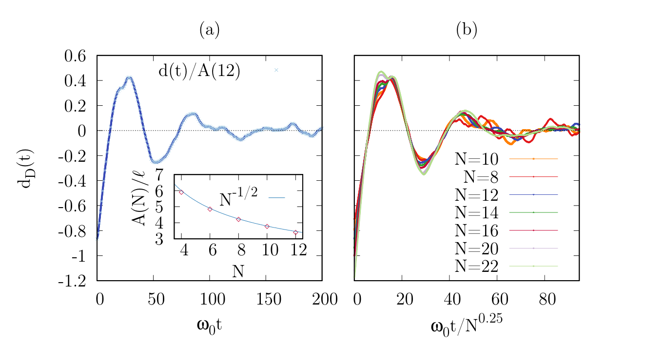
For the short time dynamics, the DMRG results for particle numbers to are presented in Fig. of the main text. In Fig. 6 we show the results for intermediate times. We first of all compare the time evolution of the discrete center of mass of the magnetization with the corresponding quantity calculated exactly in the continuum case (panel a). We find that the two curves are proportional one to the other, i.e. . The constant depends on the details of the harmonic trap and scales as (see inset in the panel a) of Fig. 6). In panel (b) of the same figure we show for different number of particles, as a function of the rescaled time . Apart from a small variation of the details of the oscillations, due to the higher number of modes involved in the dynamics, we find that curves collapse onto each other, thus confirming that the universal scaling reported in the main text holds also for larger values of .
.6 Further probes of chaoticity
We provide here further arguments on the breaking of the integrability of the model induced by the strong coupling expansion to first order in . In the spirit of Ref. Santos et al. 2012, we calculated other quantities to probe the presence of chaoticity in the system. In particular, we focused on the eigenstates of the Hamiltonian and on their localization properties. In Fig. 7 we show from left to right respectively the inverse participation ratio , the overlap between consecutive probability distribution, and the Shannon entropy . We compare the three quantities with the corresponding value predicted by the Random Matrix Theory, indicated by the green lines. By comparing the results with the ones of Ref. Santos et al. 2012, we see that the eigenstates shows some similarities in terms of statistical properties, but are not completely sparse as they would be in the integrable system.