Solar models and McKean’s breakdown theorem
for the CH and DP equations
Abstract.
We study the breakdown for CH and DP equations on the circle, given by
for , where is the mean and or respectively. It is already known that if the initial momentum never changes sign, then smooth solutions exist globally. We prove the converse: if the initial momentum changes sign, then solutions must break down in finite time. The technique is similar to that of McKean, who proved the same for the Camassa-Holm equation, but we introduce a new perspective involving a change of variables to treat the equation as a family of planar systems with central force for which the conserved angular momentum is precisely the transported vorticity. We also demonstrate how this perspective can apply to give some insights for other PDEs of continuum mechanics, such as the Okamoto-Sakajo-Wunsch equation (and in particular the De Gregorio equation).
1. Introduction
In this paper we study the - family of equations
| (1) | ||||
| (2) | ||||
| (3) |
Here is a velocity field on the circle, and defined by (3) is called its momentum or vorticity. The two special cases we care about the most are:
- •
, the -Camassa-Holm (or sometimes -Hunter-Saxton) equation, and
- •
, the -Degasperis-Procesi equation.
Our interest is in whether solutions exist for all time , or if they break down at some , given an initial condition . We will work with solutions , assuming that and .
Integrating (1) over gives, after an integration by parts, the fact that , so that for the remainder of the paper we will denote in (2)
| (4) |
If is such that in equation (4), then the breakdown picture is mostly understood by work of Sarria-Saxton [30, 31], who showed that if then all solutions of (1)–(3) are global in time; if , then there exist such that solutions break down with approaching negative infinity for some ; and for all other values of , there is an initial condition such that breakdown happens everywhere. For with , the equation becomes the Hunter-Saxton equation [15], and its explicit solution together with the geometric interpretation in terms of spherical geodesics were given by Lenells [23]. In particular all solutions break down in finite time with on a discrete set. If with , the equation (1) is the second derivative of the inviscid Burgers’ equation , for which all solutions break down in finite time as pointed out in Lenells-Misiołek-Tığlay [24]. We will review these computations in Section 2.
When the situation is more complicated: for some smooth the solution may break down, while for other smooth the solution exists globally. Here we settle the question of precisely which initial conditions lead to breakdown for the two simplest and most important special cases and . This theorem is inspired by the result of McKean [25], who proved the same for the Camassa-Holm equation, which is (1) but with (2) replaced by . Our proof is inspired by that one, and the simplified version given in [16].
The main novelty of our approach is that we introduce a new central-force model which describes the equation more geometrically. We consider a family of particles in the plane depending on , such that is zero if and only if the particle is at the origin. These particles in the plane are subject to a central force, and the conserved angular momentum is precisely the transported vorticity of the Euler-Arnold equation. Unless the central force is sufficiently large, particles with nonzero angular momentum will orbit, like planets in the solar system. However if the angular momentum vanishes, then it is possible (and relatively easy) for a particle to reach the origin in finite time. Thus if the angular momentum is always of the same sign, all particles orbit forever, while if it changes sign, then breakdown can occur. The details still depend on the particular equation, however.
Theorem 1.
Suppose the initial velocity is on , and let be the initial momentum. Assume that either or . Then the solution of (1)–(3) exists and remains in for all time if and only if never changes sign on . If does change sign, then approaches negative infinity in finite time at a value where changes from positive to negative.
The fact that or everywhere implies global existence is well-known: if it was proven in the original paper of Khesin-Lenells-Misiołek [17] which introduced the CH equation, and if it was proven in the original paper of Lenells-Misiołek-Tığlay [24] which introduced the DP equation. We give a different proof which makes a bit more clear geometrically why this works and generalizes to other equations of the form (1). On the other hand, while there are several results on sufficient conditions for breakdown of either the CH or DP equations (see e.g., [12] and [14]), they do not capture all cases. The similarity of Theorem 1 to the result of McKean suggests that a general principle applies: those equations which have the form (1) for some function , given as a pseudodifferential operator in terms of , should have breakdown behavior which depends on the sign of the initial momentum . It seems likely that with a bit more work, one can apply the technique here to similar families of PDEs to obtain the complete breakdown picture.
The special cases and in (1)–(3) are especially interesting because they are both completely integrable, with bihamiltonian structure generating infinitely many conservation laws: see [17] and [24] respectively. Aside from the conservation of average velocity (4), which is true regardless of , we have for that is constant, and for that is constant. We will not need any of the other conservation laws, which in general are not coercive. However one can use the complete integrability to obtain the global existence result, as shown in McKean [26] for the Camassa-Holm equation and sketched in Tığlay [33] for the -Camassa-Holm equation.
In Section 2, we recall the vorticity conservation formula and derive some basic properties of the model (1)–(3), including conservation laws. In Section 3 we recall the solution formulas for the simplest case of mean-zero velocity fields (for the Hunter-Saxton and Degasperis-Procesi equation) and illustrate the solar model picture of breakdown. In Section 4, we present the general transformation for nonzero and show that we obtain a central force system, where the conserved angular momentum is precisely the vorticity. In Section 5 we present the local existence theory, showing in particular when that the solution exists in the transformed coordinates up to and slightly beyond the first time a particle reaches the origin; when the solution exists for all time in the transformed coordinates. In Section 6 we prove that the central force is bounded polynomially in time, and we prove some general aspects of mechanics under central forces (not necessarily coming from a solar model of a PDE). These are used in Section 7 to prove Theorem 1. Finally in Section 8, we discuss a different transformation of equation (1) (where the momentum is given by instead of (2)) and illustrate how the solar picture here generates bounds for the solution; this is the Okamoto-Sakajo-Wunsch family of equations, a generalization of the De Gregorio equation which appears in a particularly simple way here.
The author thanks Martin Bauer, Boris Khesin, Alice Le Brigant, Jae Min Lee, Stephen Marsland, Gerard Misiołek, Cristina Stoica, Vladimir S̆verák, Feride Tığlay, and Pearce Washabaugh for very valuable discussions, as well as all the organizers and participants of the BIRS workshop 18w5151 and the Math in the Black Forest workshop for listening to early versions of this work. The work was done while the author was partially supported by Simons Foundation Collaboration Grant #318969.
2. Background
Equation (1), for a general defined by a pseudodifferential operator in terms of , is a generalization of the Euler-Arnold equation. For it is exactly the Euler-Arnold equation: it describes the evolution of geodesics under a right-invariant Riemannian metric on the diffeomorphism group of the circle, where the metric is given at the identity by
| (5) |
If is positive-definite, this defines a Riemannian metric, and the actual geodesic in the diffeomorphism group is found by solving the flow equation
| (6) |
Paired with (1), this is a second-order differential equation for ; the decoupling is an expression of Noether’s theorem due to the right-invariance. The Camassa-Holm equation with is the best-known example in one dimension; in higher dimensions one gets the Euler equations of ideal fluid mechanics and a variety of other equations of continuum mechanics. See surveys in [2], [18], [20] for other examples. When and is nonnegative but not strictly positive, the equation may describe geodesics on quotient spaces of , modulo a quotient group generated by the kernel of ; see Khesin-Misiołek [19] for the requirement. Examples include the Euler-Weil-Petersson equation [13] and the Hunter-Saxton equation.
For other values of , the quadratic form (5) is not necessarily conserved, and if not then the equation (1) does not represent the equation for geodesics in a Riemannian metric. However it can still be interpreted as a geodesic for a right-invariant but non-Riemannian connection; see [17] and [11] for details on this construction in the present cases, and [34] for the general situation. A well-known example is the Okamoto-Sakajo-Wunsch equation [28], where in terms of the Hilbert transform (if it becomes the well-known De Gregorio equation [7]) which are considered the simplest one-dimensional models for vorticity growth in the 3D Euler equation. We will return to this family at the end of the paper. On the other hand if then (1) is the generalized Proudman-Johnson equation, studied in [30, 31], which is related to self-similar infinite-energy solutions of the Euler equations of fluids.
What all these equations have in common is the conservation of vorticity property, which we describe as follows.
Proposition 2.
For any equation of the form (1), regardless of how is related to , we have the vorticity transport formula
| (7) |
.
Proof.
Observe that by the chain rule and the definition (6) of , we have
| (8) |
Furthermore differentiating (6) in yields
| (9) |
Using both in (1) shows that
which shows that the vorticity is transported via (7). This is a consequence only of (1), and is true regardless of whether is related to by (2) or not. ∎
As long as remains a diffeomorphism of the circle, we will have , so that the sign of is preserved: for each , the transported vorticity along the Lagrangian path is positive if and only if the initial vorticity is positive. Equation (7) can be inverted to solve for in terms of and , and from there we may obtain a first-order equation for using (6). We will not take this approach directly. Instead we study the second order system (1)–(3), (6) by an approximate linearization. That is, we differentiate (9) in time to get a second order equation for , then change variables to simplify it. We will elaborate on the differential geometric meaning of this at the end of the paper.
Proposition 3.
Proof.
Plugging the formula into (1) gives
| (11) |
Integrate this over : all terms integrate to zero by periodicity, and we obtain , as mentioned in the Introduction.
Now find the antiderivative in of the remaining terms in (11), and we obtain (10) for some function . Integrating both sides over the entire circle shows that
| (12) |
Differentiation of (12), using (10), gives
after noticing the first two terms vanish and the third term can be integrated by parts to combine with the fourth term.
In particular when we have that is constant, and thus so is . On the other hand, when , we get , which is constant since is. ∎
It is the form (10) of the equation, which makes sense for , that we will view as fundamental. We will see that the kinetic energy term defined by (12) controls the global behavior of solutions. This is precisely the reason why our technique will work well in those two cases, and the lack of a bound on is the reason we cannot yet prove Theorem 1 for other values of . (As will be clearer later, a polynomial growth bound for in would be sufficient to prove Theorem 1, but the obvious successive-differentiation manipulations seem to yield at best exponential growth.)
As is typical with equations of Euler-Arnold type (as first noticed by Ebin-Marsden [9]; see also [6] and [27]), the equation is best-behaved in terms of the flow , i.e., using the Lagrangian description. To see this here, differentiate (9) with respect to to get
Using this, equations (10)–(12), after composing with and using (6) and (9), become
| (13) |
We are going to view this as an equation for , in spite of the fact that must be determined nonlocally by the spatial integral of ; this is an unavoidable complication. Now the term in square brackets is relatively easy to control (at least if or ), while the first term on the right side of (13) is of higher order and more likely to become singular. The trick is thus to change variables to eliminate it, and end up with an equation that is nearly linear. We will first analyze this in the simplest case where and , and generalize from there.
3. Solar models for H-S and D-P equations
Let us recall the analysis of the equations when and or , when everything can be done explicitly. The results here are well-known, but our perspective is new. The easiest case is (solved in [24]), where (13) becomes . Define and . Then we have
which is a trivial central force system (with no force). Conservation of angular momentum of this system follows from
and the solutions are given by and . These obviously exist for all time, and remains positive for ; hence also remains positive here. For larger , the function becomes negative, which means that is not invertible as a function of : it maps multiple values of to the same point. This leads to our inability to invert the formula to find , which is the shock phenomenon: the solution is not even continuous. Note however that exists and remains as spatially smooth as for all time, another illustration of the fact that things are better in Lagrangian coordinates.
The more interesting case is and . Here equation (13) becomes
| (14) |
Define ; then equation (14) becomes
Here is constant in both space and time, and we have simple harmonic motion. Defining , we clearly also have
Since and , the fact that and yields the initial conditions
The solutions with these initial conditions are
We can easily see that remains positive for
and becomes negative beyond that. However since in this case, we will find for typical initial data that is positive for all except a discrete set of points (depending on ), which means will be a homeomorphism even if it not a diffeomorphism. This allows us to define as a continuous function, although its derivative will approach negative infinity wherever by (9). Note that again the central force system has conserved angular momentum, now given explicitly by
This is the reason for the scaling on . In Figure 1 we demonstrate what this looks like for a simple solution of the Hunter-Saxton equation.


Remark 4.
We see that breakdown is very different already between and . One might have expected that since only appears as a coefficient of lower-order terms in the PDE (10), it does not have a large role in the breakdown picture. However if we have global weak solutions which remain continuous (and the corresponding typically remains a homeomorphism even if it is not a diffeomorphism). In fact if we consider all weak solutions that conserve energy, the family found here is unique [32]. On the other hand if , the solution must become discontinuous, and as is well known the solution is no longer unique without an extra entropy condition.
4. The general transformation
In the cases of the last section, we have seen that for each fixed , the functions and form the components of a central-force system, which implies that the angular momentum is always conserved. This conserved quantity is precisely the transported vorticity, so that the conservation law (7) is encoded here automatically. This fact is what ensures that when the vorticity is always positive or always negative, classical solutions will be global; see Theorem 15. The intuition is that the system is attracted or repulsed by a central force, analogously to the sun’s gravity, and singularities correspond to the particle reaching the sun in finite time. As in our solar system, this can only happen if the particle dives directly into it, and any nonzero angular momentum prevents this. A very singular force may still lead to finite-time collapse, but in our situations the force is bounded on finite time intervals. We will now show how to obtain this picture in the general case when and is any real number.
Theorem 5.
Proof.
Since for all , note that we always have
| (23) |
The formula (16) is a straightforward computation from (13): the transformation gives
so that eliminates the quadratic term from the equation. We then obtain
| (24) |
The formula for is determined from the fact that we know
| (25) |
as well as the fact that
| (26) |
and these two conditions clearly uniquely determine . The condition (26) comes from the change of variables formula and (4): we have
We can easily compute that defined by formula (20) satisfies both requirements, using the formula (23), and so (24) becomes (16).
The forcing term defined by (18) appearing in (16)–(17) depends on the solution and (or if we like on and , since we can in principle reconstruct from if desired). As such we properly view (16) as an ODE on a Banach space. Fortunately the dependence of on and is relatively simple, and is well-behaved even if has only limited smoothness—for example if and are in for some integer , then the function will be in . More importantly, the map from is actually as a map of Banach spaces as long as remains positive (which is only needed for the power function to be smooth). Hence equation (16) describes a ODE on the space of functions satisfying
| (27) |
where the integral condition comes from (23). If happens to be an integer, as it does for and , we get smoothness even for functions that may be zero or negative at some points, and this allows us to extend the ODE to the larger space
As we are interested in the breakdown of the equation when , allowing to approach zero (and even continue to go negative) gives us global solutions in the new coordinate, which translate into weak solutions when we invert to get , and from this and .
Corollary 6.
Proof.
The fact that angular momentum is conserved for central force systems is well-known: it follows from
Equation (15) implies that
so that
At time , the right side is . ∎
5. Local and global existence in the transformed variables
Because the transformation to Lagrangian coordinates eliminates the loss of derivatives (essentially just being able to combine terms like into as in equation (8)), we get a smooth ODE on the space of functions . We want to work in the simplest space for which all the functions make sense, so we will require that be in order to have the momentum be continuous. We then expect to be in for short time, which by the flow equation (6) should imply that is also spatially in ; hence would be in and would be in . Working in these spaces, we thus get existence of solutions using Picard iteration. The following was proved for the case by Deng-Chen [8], following the technique of Lee [22] for the Camassa-Holm equation. The proof for other values of is similar, and just involves showing that defined by (18) is smooth as a function of and .
Theorem 7.
Proof.
The main point is to write it as a first-order system with , viewing , , and as functions not of but of . That is, we write given by (18) as
where from equation (20) and from (19) are given by
and
As long as remains strictly positive, and are smooth functions of . For example, the derivative of is
which depends continuously on the functions , and further derivatives can be computed the same way. Similarly the derivative of can be computed, and for any functions , the derivative map will also be a function (actually since is smoothing, but we don’t need that).
The only thing that remains is to check that the integral constraint
is a submanifold of , where denotes the functions on with strictly positive image; this is easy by the usual implicit function theorem for Banach spaces. Then we verify that the differential equation preserves these constraints, which is straightforward, and shows that our smooth vector field actually descends to a vector field on the submanifold. For details about the implicit function theorem and vector fields on Banach manifolds, see for example Lang [21] or Abraham-Marsden-Ratiu [1]. ∎
The local existence proof works for any value of , but for global existence we only have a proof in case , because that is the case where we know conservation laws to get global bounds on solutions. Even when we cannot prove global existence since the conservation law only applies when is a diffeomorphism, and by Remark 4 we cannot expect good ODE behavior in any coordinates: even when the equation genuinely breaks down without a unique global weak solution, since must go negative. But this will demonstrate that for example and cannot approach infinity. In case proofs were given in Deng-Chen [8] and in Tığlay [32], so we will only treat the case . The essential thing here is the formula (10), which for becomes
| (29) |
with the constant of integration in chosen so that it has mean zero, since the left side must integrate to zero. The conservation law
| (30) |
proved in [24] is one of the infinite family of conservation laws for , and although it is not very strong, it is enough to get a bound on , which allows us to control the growth of pointwise, at least as long as remains a diffeomorphism and for a (possibly small) time beyond. This strategy comes from [12].
Theorem 8.
Proof.
In the case , the transformation (15) simplifies to just . The easiest way to proceed is to show that itself satisfies a differential equation for which the right side is bounded. Equation (24) becomes
| (31) |
and integrating once more in space gives
| (32) |
where is essentially a pressure function, related to from (29) by . is defined uniquely by the conditions
Suppressing time dependence, we can write explicitly in terms of and by
For periodic , this defines a periodic function which depends smoothly on , since it involves only products and continuous integral operators. Furthermore because there is no composition with , this still makes sense even if stops being a homeomorphism.
The conservation law (30), together with the conservation of the mean from (4), implies that is constant in time, and in Lagrangian form this becomes
| (33) |
which again makes sense even if is not positive. As long as remains nonnegative, we obtain from the mean-zero condition the bound
using (33) and the fact that is periodic.
Hence as long as remains nonnegative, we have that is bounded in the norm uniformly in time. Equation (32) now implies that is uniformly bounded in time, and we conclude that grows at most linearly in time (again as long as remains nonnegative). Equation (31) now implies that satisfies an estimate of the form
In particular the right side of the differential equation is bounded on all finite time intervals in the space of diffeomorphisms . Thus by the usual theory of ODEs in Banach spaces, e.g., Proposition 4.1.22 in [1], the solution can be continued for as long as remains nonnegative. In particular the local existence theorem gives some small such that the solution can be continued on the interval , beyond the time where first reaches zero.
Differentiating equation (31) in gives, by the same reasoning, an ordinary differential equation for with uniform bounds in the supremum norm; hence a initial condition leads to a solution , and thus a solution . The fact that we also have a solution is now straightforward, since satisfies the linear ODE (17) with known coefficients in terms of the function . ∎
This theorem establishes that the only thing that can go wrong with the global solutions of equation (13) in the cases and is that approaches zero. Significantly, the equation for in the form (31) depends only on as a function on of some smoothness, but not on the fact that is a diffeomorphism. Hence the local existence result for the ODE holds even when reaches zero, and we get existence for some (possibly small) time beyond that. The difficulty is that without a global bound on the energy, we cannot extend this for all time.
Again we note that in the case the breakdown is completely understood: when , the function ceases even to be a homeomorphism as becomes negative, while if the fact that means that always, so that typically will remain a homeomorphism. Since , this is the difference between the solution having shocks where it must cease being continuous, as opposed to steepening where remains continuous but its slope may approach infinity due to equation (9). For other values of things may be much worse: Sarria and Saxton [30] showed that for or , there are solutions for which approaches either zero or infinity, everywhere at the breakdown time. The reason here is that for or , the terms in the forcing function defined by (18) are well-controlled in time, while in general there are no good estimates for the growth. In the next section we will see what consequences can be found if we can obtain a global bound on the central force.
6. Properties of central force systems with bounded forcing terms
Bounds for the central force (not necessarily uniform, but with controlled growth in time) are crucial for what comes next. We first record the bounds we can obtain in the cases , then derive some consequences that apply to any central force system (not merely those arising from Euler-Arnold equations).
Lemma 9.
Proof.
In the case , we have already established this in the proof of Theorem 8, since there
and grows at most linearly in time because is bounded. In the case , the forcing function is given by
and is constant in time for , and given by
This implies that is constant in time, and we thus get a uniform bound for by the Poincaré inequality, since
and the right side is constant in time. ∎
One might hope that a polynomial-in-time bound like this is true for other values of ; if it were, the technique of the breakdown proof we will give later would also show the same breakdown phenomenon for all values of . Ultimately the only thing we need is that the forcing function grows like a polynomial in time, because it will be less than the exponential decay we get in general from the equation whenever . If we could establish any kind of polynomial estimate for the energy given by (19) for other values of , we would obtain the same breakdown result here proved for and . However the fact that Sarria-Saxton [30] showed that the basic breakdown mechanism changes when makes clear that this could only be hoped for if .
The main tools we use to establish breakdown are the following simple result which applies for any ODE for fairly general forcing functions (and thus will apply here for the individual particles for each individual ). The first lemma gives an upper bound for the solution in terms of the forcing function, while the second establishes that solutions will eventually reach zero if their velocity is sufficiently negative. Our philosophy is that although the forcing function depends implicitly and nonlocally on the solution for all values of , each individual particle feels a force that is some given function of time, bounded on finite time intervals, and thus we can treat it as essentially an external force.
Lemma 10.
Suppose satisfies the second-order ODE
on some interval , where may be infinite, and assume for some nonnegative differentiable increasing function .
Then there is a such that
| (34) |
for all .
Proof.
Define . Then satisfies the Riccati inequality
| (35) |
If is ever larger than , then must decrease; thus if , then for all time until possibly crosses . If is smaller than , then the difference satisfies
In particular if is ever positive, it will always be positive. This shows that for all time if it is true for any time. Combining shows that
which is equivalent to (34). ∎
Lemma 11.
Suppose
| (36) |
for some continuous function on a maximal time interval . If and is sufficiently negative, then for some .
Proof.
Let denote the solution of (36) satisfying
If reaches zero in finite time, then by the Sturm comparison theorem, must also reach zero whenever .
Otherwise is always positive, and the general solution of (36) is given by
as can easily be verified by direct substitution. (This is just reduction of order.) The function will turn negative for some as long as
∎
The next result tells us about the effect of nonzero angular momentum. It is familiar from basic celestial mechanics: even for a not-too-singular force directed toward the origin, a particle will not reach the origin if there is nonzero angular momentum, while a particle with zero angular momentum will reach the origin in finite time. In our context this will give a lower bound on the radial coordinate , which gives global existence in Theorem 15 if the angular momentum is never zero.
Lemma 12.
Suppose is a planar system satisfying the ODE
| (37) |
where is continuous and bounded on . Let
| (38) |
Then if is nonzero, cannot reach zero on .
Proof.
Conservation of angular momentum ensures that
so that
We then obtain
Observe that can only be made small if it is decreasing on some interval , so to get an upper bound on this energy we define
Then for all and , and integrating over assuming that on gives
In particular we obtain
and in particular is positive since is finite by assumption.
There can only be finitely many such intervals where can decrease on since can only decrease when either or is decreasing, and a linear differential equation with bounded force coefficient can only have a discrete set of turning points in a compact interval. ∎
Remark 13.
Of course, if we allow the forcing function to be something like , then the particle can reach zero in finite time. The change of time variable in this case turns each equation in the system (37) into
which will have infinitely many oscillations up to if and only if . Thus if the system will spiral around the origin infinitely many times until reaching the origin at . For bounded , things are substantially simpler, but note that we only have reasonable bounds on in special cases (in particular and in the present context).
One further lemma simplifies our considerations, which is the reflection symmetry of the equation (1)–(3). Note that since , and must change sign if is not constant, the condition that changes sign has somewhat different consequences for the convexity of depending on whether is positive or negative. However these are illusory, and the following proposition shows that if , we can assume without loss of generality. This proposition is well-known and appears in many places, e.g., in [12].
Proposition 14.
Proof.
In light of Proposition 14, we will always assume that without loss of generality.
7. Proof of Theorem 1
First we show that if the momentum is everywhere positive or everywhere negative, then the solution of equations (1)–(3) exists globally and gives a diffeomorphism. This result is already contained in the original papers [17] and [24], based on analytic inequalities (and generalized for any value of in [34]), but our perspective here is different. By Proposition 14, we may assume without loss of generality that the initial momentum is strictly positive.
Theorem 15.
Proof.
By the definitions (15) of and , the first time approaches zero, we must simultaneously have approaching zero, since
Because is positive everywhere until it approaches zero, its minimum is also approaching zero, so that is approaching zero at the same time; meanwhile the second term in approaches zero since remains bounded and the integral is multiplied by . Hence the only way can ever reach zero is if both and approach zero simultaneously.
Theorem 8 shows that for or , the only way the solution can break down is if reaches zero at some finite time , and when this happens we still have at least local existence in coordinates beyond this . By Lemma 12, since is positive and is bounded by Lemma 9, the quantity cannot reach zero on , and we get a contradiction. ∎
Now we consider what happens when the sign of the momentum changes. By Proposition 14, we may assume without loss of generality that . In this case, the assumption that momentum changes sign means that for some values of , because it would always be true that for some values of (for example when has a local maximum or minimum). The important thing here becomes which in particular implies that is convex on some interval. This leads to a convexity result on the function , and it is on this that all our breakdown results depend.
Our strategy will be as follows: we choose points such that on : then we establish that
- •
has an upper bound independent of in Lemma 16;
- •
decays like for some in Lemma 17;
- •
and thus can be made as small as we want in Lemma 18,
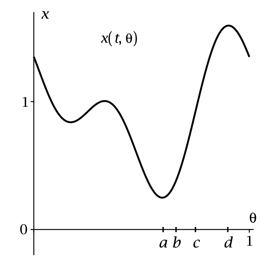
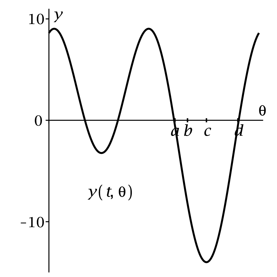
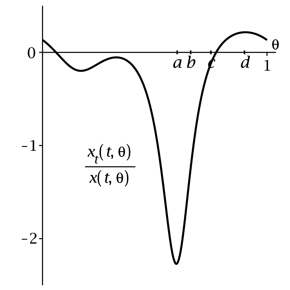
and from this we use Lemma 11 to show that must reach zero in finite time. None of the choices of these points actually matter, although optimizing the choice could lead to a better estimate for the breakdown time. All that matters is that and are chosen so that on , which we will assume from now on. Essentially all three lemmas rely on the same basic conservation-of-momentum equation
| (39) |
which is a direct consequence of the equation (28). We apply it in three different ways: integrating in time for Lemma 16, integrating in both time and space for Lemma 17, and integrating in space only for Lemma 18. The first two lemmas are basically the same as arguments in the original paper of McKean [25], while the third is a new argument. See Figure 2 for the heuristic in a simple case.
Lemma 16.
Proof.
The next step is to integrate equation (41) over , which gives a bound on the logarithm of . This implies exponential decay in time of .
Lemma 17.
Consider all the same hypotheses as in Lemma 16 on an interval . Then for any with , the function satisfies
| (43) |
and is a constant depending only on .
Proof.
The last step is to use the conservation of angular momentum formula (28)
directly. Dividing through by gives
| (45) |
Now by Lemma 10, since both and satisfy the same ODE with a bounded forcing function, the quantity is bounded above by the square root of any increasing upper bound for the forcing function. Meanwhile since is negative if and only if is, the other term can be made as large and negative as we want when and are both small.
Proof.
Integrating equation (45) for , we obtain
where is the positive quantity
| (47) |
We want to establish a lower bound for .
Combining Lemmas 16–18, we can now prove the second half of Theorem 1. Everything here would in fact work for any value of , not just or , except for the fact that we need a subexponential upper bound for the forcing function in order to use Lemma 10.
Theorem 19.
Proof.
Choose any subdivision such that is negative on , and such that . Lemma 16 implies that
Lemma 17 then implies that
where is given by equation (43). Applying Lemma 18 then gives
where is given by (46).
Since satisfies the equation by Theorem 5, the quantity is bounded above by an estimate of the form
| (49) |
where is any positive increasing function satisfying for all and , as in Lemma 10. If or , we can use Proposition 9 to see that grows at most polynomially in time, for each value of , and this implies by Lemma 10 that grows at most polynomially in time. Integrating over the interval still gives polynomial growth in time, and this implies that our estimate takes the form
where is a function growing at most like a power of . Since the exponential term eventually dominates, we see that we can make the integral
as small as we want, which also implies that for some , the quantity can be made as small as desired. For such , Lemma 11 implies that must reach zero in finite time. Of course, since is increasing on , the smallest value must occur at , when the sign of changes from positive to negative. ∎
8. Outlook
The general principle that or everywhere implies global existence of classical solutions for solutions of (1) is established in Tığlay-Vizman [34] as long as the definition of in terms of that replaces (2) involves at least two derivatives of . In many situations of interest, the operator has mean zero for all , and so it is impossible for to have a constant sign; thus we would expect all classical solutions to break down in finite time. As an example we return to the Okamoto-Sakajo-Wunsch equation [28], given by (1) where , for which integrates to zero, and it is impossible to have positive or negative everywhere. (On the real line the situation is different, but our periodic context forecloses such possibilities.)
The following construction was presented in [3] in the case , but most things work the same way for any value of . Breakdown for all solutions in the case was given in [29], while breakdown for all positive with odd was given by Castro-Cordóba [4]. For , all solutions break down in finite time, while for the solution is much more complicated and unknown in general (particularly in the most important case , the De Gregorio equation). For the state of the art on global existence and breakdown for such equations, see Chen [5] for the periodic case, Elgindi-Jeong [10] for the nonperiodic case, and references in both.
Proposition 20.
Suppose and satisfy (1) with momentum defined by , i.e., the modified Constantin-Lax-Majda equation. Define the transformation
| (50) |
where is defined by
| (51) |
Then satisfy a solar model of the form
where is always positive.
Proof.
This formulation makes it obvious that if , the force is attracting, and zero angular momentum with and implies reaches zero in finite time. Hence does as well. (There is always such a by the Hopf Lemma; see [29].)
If , the effective force in the solar model becomes repulsive. The singular condition for is no longer that , but rather that . This again translates into . (This corresponds to approaching positive infinity rather than negative infinity.) It is still possible that the particle can approach the origin, but it needs to have both zero angular momentum and a sufficiently negative velocity pointing toward the origin to counteract the repulsive force.
We give a simple example of a bound that is straightforward in the solar model.
Corollary 21.
Proof.
In case , equation (53) takes the form
Positivity of means that is strictly positive, and this implies that while may possibly decrease on some interval , it must eventually increase, and once it begins to increase it must continue.
If for some we know that is decreasing on and increasing for , then we compute (at fixed ) that
On the right side is nonpositive, and we obtain
In particular we have
Since must continue to increase for , this is indeed the minimum possible value of on the maximum time interval of existence.
Since , we conclude that is bounded above by
on the maximum time interval of existence. ∎
Obviously Corollary 21 is only useful when , and by definition of our momentum operator , there will certainly be points where . However such estimates could be useful for estimating the forcing function , which depends nonlocally on our variables. (Note that bounds on were derived in [29].) We leave further analysis for future research, but the point is that the general framework here relates a family of Euler-Arnold-type PDEs to a well-understood central force system, which makes some phenomena regarding breakdown or global existence easier to intuitively understand.
The reason this approach works is because the equations are “nearly” linear in terms of the variable . Of course the coefficients of this equation depend on , and a transformation may eliminate some of this dependence (e.g., quadratic terms like can be eliminated by a power transformation). This is due to the fact that satisfies some kind of geodesic equation of the form for some Christoffel map , which is bilinear and symmetric in the last two variables but typically depends in a complicated way on the first. Differentiating this with respect to any parameter leads to the Jacobi equation for the variation. In infinite dimensions the spatial variable itself can always be treated as this variational parameter, so that always satisfies the Jacobi equation. The coefficients and covariant derivative here depend on (and thus indirectly on ), so we cannot view this as a true linear equation, but if the curvature is bounded or well-understood, this equation may be easy to analyze. These are the situations we have studied here. The fact that equation (1) applies to many situations of continuum mechanics suggests that this technique may produce new insights that are not obvious from direct PDE techniques.
The author states that there is no conflict of interest. No data was produced for this paper.
References
- [1] R. Abraham, J.E. Marsden, and T. Ratiu, Manifolds, tensor analysis, and applications, second edition, Springer-Verlag, New York, 1988.
- [2] V. Arnold and B. Khesin, Topological nethods in hydrodynamics, second edition, Springer-Verlag, New York, 2021.
- [3] M. Bauer, B. Kolev, and S.C. Preston, Geometric investigations of a vorticity model equation, J. Differential Equations, 260 no. 1, pp. 478–516 (2016).
- [4] A. Castro and D. Córdoba. Infinite energy solutions of the surface quasi-geostrophic equation, Adv. Math., 225 no. 4, pp. 1820–1829 (2010).
- [5] J. Chen, On the regularity of the De Gregorio model for the 3D Euler equations, arXiv:2107.04777 (2021).
- [6] A. Constantin and B. Kolev, On the geometric approach to the motion of inertial mechanical systems, J. Phys. A: Math. Gen. 35, pp. R51–R79 (2002).
- [7] S. De Gregorio, On a one-dimensional model for the three-dimensional vorticity equation, J. Stat. Phys. 59, pp. 1251–1263 (1990).
- [8] X. Deng and A. Chen, Global weak conservative solutions of the -Camassa-Holm equation, Bound. Value Probl. 2020 no. 33 (2020).
- [9] D.G. Ebin and J. Marsden, Groups of diffeomorphisms and the motion of an incompressible fluid, Ann. Math. 92 no. 1, pp. 102–163 (1970).
- [10] T.M. Elgindi and I.-J. Jeong, On the effects of advection and vortex stretching, Arch. Rat. Mech. Anal. 235 pp. 1763–-1817 (2020).
- [11] J. Escher and B. Kolev, The Degasperis–Procesi equation as a non-metric Euler equation, Math. Z. 269, pp. 1137-–1153 (2011).
- [12] Y. Fu, Y. Liu, and C. Qu, On the blow-up structure for the generalized periodic Camassa-Holm and Degasperis-Procesi equation, J. Funct. Anal. 262 pp. 3125–3158 (2012).
- [13] F. Gay-Balmaz and T.S. Ratiu, The geometry of the universal Teichmüller space and the Euler–Weil–Petersson equation, Adv. Math. 279, pp. 717–778 (2015).
- [14] G. Gui, Y. Liu, and M. Zhu, On the wave-breaking phenomena and global existence for the generalized periodic Camassa–Holm equation, Int. Math. Res. Not. 2012 no. 21, pp. 4858–4903 (2012).
- [15] J. K. Hunter and R. Saxton, Dynamics of director fields, SIAM J. Appl. Math. 51 1498–-1521 (1991).
- [16] Z. Jiang, Y. Ni, and L. Zhou, Wave breaking of the Camassa–Holm equation, J. Nonlinear Sci. 22 pp. 235–245 (2012).
- [17] B. Khesin, J. Lenells, and G. Misiołek, Generalized Hunter–Saxton equation and the geometry of the group of circle diffeomorphisms, Math. Ann. 242 no. 3, pp. 617–656 (2008).
- [18] B. Khesin, J. Lenells, G. Misiołek, and S.C. Preston, Curvatures of Sobolev metrics on diffeomorphism groups, Pure Appl. Math. Q. 9 no. 2, pp. 291–332 (2013).
- [19] B. Khesin and G. Misiołek, Euler equations on homogeneous spaces and Virasoro orbits, Adv. Math. 176 no. 1, pp. 116–144 (2002).
- [20] B. Khesin and R. Wendt, The geometry of infinite-dimensional groups, Springer-Verlag, Berlin, 2003.
- [21] S. Lang, Differential and Riemannian manifolds, Springer-Verlag, New York, 1995.
- [22] J.M. Lee, Geometric approach on the global conservative solutions of the Camassa–Holm equation, J. Geom. Phys. 142, pp. 137–150 (2019).
- [23] J. Lenells, The Hunter-Saxton equation describes the geodesic flow on a sphere, J. Geom. Phys. 57, pp. 2049–2064 (2007).
- [24] J. Lenells, G. Misiołek, and F. Tığlay, Integrable evolution equations on spaces of tensor densitites and their peakon solutions, Commun. Math. Phys. 299, pp. 129-–161 (2010).
- [25] H.P. McKean, Breakdown of a shallow water equation, Asian J. Math. 2 no. 4, pp. 867–874 (1998).
- [26] H.P. McKean, Fredholm determinants and the Camassa-Holm hierarchy, Comm. Pure Appl. Math. 56 no. 5, pp. 638–680 (2003).
- [27] G. Misiołek, Classical solutions of the periodic Camassa-Holm equation, Geom. Funct. Anal. 12, pp. 1080–1104 (2002).
- [28] H. Okamoto, T. Sakajo, and M. Wunsch, On a generalization of the Constantin–Lax–Majda equation, Nonlinearity, 21 no. 10, pp. 2447–-2461 (2008).
- [29] S.C. Preston and P. Washabaugh, Euler-Arnold equations and Teichmüller theory, Differential Geom. Appl. 59, pp. 1–11 (2018)
- [30] A. Sarria and R. Saxton, Blow-up of solutions to the generalized inviscid Proudman–Johnson equation, J. Math. Fluid Mech. 15 no. 3, pp. 493–523 (2013).
- [31] A. Sarria and R. Saxton, The role of initial curvature in solutions to the generalized inviscid Proudman-Johnson equation, Quart. Appl. Math, 73 no. 1, pp. 55–91 (2015).
- [32] F. Tiğlay, Conservative weak solutions of the periodic Cauchy problem for HS equation, J. Math. Phys. 56 no. 2, 021504 (2015).
- [33] F. Tiğlay, Integrating evolution equations using Fredholm determinants, Electron. Res. Arch. 29 no. 2, pp. 2141–2147 (2021).
- [34] F. Tiğlay and C. Vizman, Generalized Euler-Poincaré equations on Lie groups and homogeneous spaces, orbit invariants and applications, Lett. Math. Phys. 97 no. 1, pp. 45–60 (2011).