Phase Spectrometry For High Precision mm-Wave DoA Estimation In 5G Systems

Given noise is Gaussian and independent for each PIM, Fisher information matrix (FIM) of $\Delta\phi$ with respect to an arbitrary vector $\boldsymbol{x}$ , e.g. unknowns to be estimated, can be derived as [39]

	$\displaystyle\sum_{\mathbb{P}}\frac{1}{\sigma^{2}}\nabla_{\boldsymbol{x}}\Delta\phi^{H}\nabla_{\boldsymbol{x}}\Delta\phi=$	$\displaystyle\sum_{\mathbb{P}}\frac{1}{\sigma^{2}}(-j2\pi f_{c}\nabla_{\boldsymbol{x}}(\Delta(t))^{H}be^{-j2\pi f_{c}\Delta(t)})(j2\pi f_{c}\nabla_{\boldsymbol{x}}\Delta(t)be^{j2\pi f_{c}\Delta(t)}))=$
		$\displaystyle\sum_{\mathbb{P}}\frac{4b^{2}\pi^{2}f^{2}_{c}}{\sigma^{2}}\nabla_{\boldsymbol{x}}\Delta(t)^{H}\nabla_{\boldsymbol{x}}\Delta(t)\,,$		(3)

where $\mathbb{P}$ is the set of all PIMs, and $\nabla_{\boldsymbol{x}}$ is the gradient operator with respect to (w.r.t) $x$. Therefore, FIM of PIM is exactly equals to the following observations,

$$\delta(t)=b\Delta(t)+\frac{v_{s}}{2\pi f_{c}}\,.$$

(4)

where $\delta(t)$ is an observation of TDoA of signal between two antennas. Therefore, PIM with additive white noise power $\sigma^{2}$ equals to TDoA observations with additive white noise power $\frac{\sigma^{2}}{4\pi^{2}f^{2}_{c}}$ of the same PIA in the fisher sense. Assuming far field criteria is fulfilled [40], we have

$$\delta(t)=b\frac{D}{c}cos(\theta_{A})+\frac{v_{s}}{2\pi f_{c}}\,,$$

(5)

where $c$ is the speed of light and $\theta_{A}$ is DoA of signal and $D$ is the gap between two antennas. CRLB of $\theta_{A}$ estimation based on measurements as of (5) can be derived as follows

$$\mathrm{CRLB}_{\theta_{A}}=\frac{\frac{\sigma^{2}_{s}}{b^{2}}}{(\frac{D}{c}2\pi f_{c})^{2}sin^{2}(\theta_{A})}=\frac{\frac{\sigma^{2}_{s}}{b^{2}}}{(\frac{2\pi D}{\lambda})^{2}sin^{2}(\theta_{A})}\,.$$

(6)

Now lets take a look at CRLB of DoA estimation using a ULA in which antennas are placed half wavelength apart [41],

$$\mathrm{CRLB}_{\theta_{A}}=\frac{6\frac{\sigma^{2}_{s}}{b^{2}}}{\pi^{2}m(m^{2}-1)sin^{2}(\theta_{A})}\approx\frac{6\frac{\sigma^{2}_{s}}{b^{2}}}{\pi^{2}m^{3}sin^{2}(\theta_{A})}\,,$$

(7)

where $m$ is the number of array elements. Given the same SNR, DoA estimation using PIM and a ULA array are equivalent in the Fisher sense when,

$$m=(24)^{\frac{1}{3}}(\frac{D}{\lambda})^{\frac{2}{3}}\approx 2.8845(\frac{D}{\lambda})^{\frac{2}{3}}\,.$$

(8)

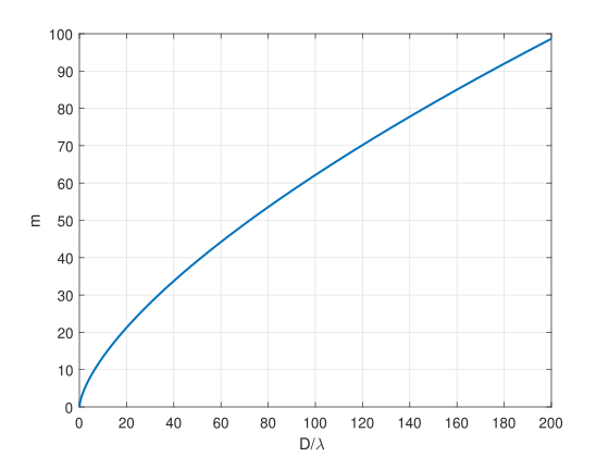
Figure 2 illustrates (8), as an example, DoA estimation using a PIA with $\frac{D}{\lambda}=200$ is equivalent to a ULA with 100 elements in the Fisher sense. Consequently, DoA estimation using PIM with gap $D$ between two antennas equals to DoA estimation exploiting a ULA with $m$ antennas placed half wavelength apart, in which $m$ obeys (8). This could lead to a huge reduction in complexity of the antenna array required for high precision DoA estimation -that reduces the required number of antennas from $m$ to 2-; if so, why is it not a common DoA estimation technique now? it is because DoA estimation using PIM is ambiguous and there are a number of different DoAs that can be inferred from a specific PIM [42]; As $D$ increases CRLB decreases, however, ambiguity escalates. Moreover, DoA estimation using PIM is not capable of detecting and discriminating between multiple concurrent DoAs. In section IV, we propose a solution to estimate DoA using PIMs observed for multiple frequencies, instead of only measuring PIM for only a single frequency. We will see that this approach not only leads to PIM disambiguation, but also provides us with DoA estimation of all signal propagation paths between the source and the device.

In this section, we explain why DoA estimation precision and antenna beam-width are not necessarily coupled, which further proves that spatial division (SD) and IA can be considered and performed as two completely independent tasks. Referring to (6) and (7), CRLB of angle estimation precision is directly related to SNR, as SNR increases precision improves; in other words, we can obtain any arbitrary precision if SNR is high enough regardless of $m$ or $D$. Although SNR can be improved by increasing the number of antennas, in a ULA, it can also be improved by integration, which is the time interval we can coherently receive and integrate a signal. Equivalently, angle precision can be improved only by integration, which come at a time cost, regardless of $m$ or $D$.

Now let’s take a look at angle resolution concept. Angle resolution help us to measure the capability of a technique to discriminate between multiple incoming signals from different DoAs. We define angle resolution as the minimum angular distance between two incoming signals that can be discriminated by a technique. Angle resolution is directly coupled with SD capability of a technique. A ULA can discriminate between two DoA if their angular distance is more than it’s beam-width. Similarly, in the transmit mode, if the angular distance between two users is more than the beam-width and antenna sends signal to one of them, it causes much less interference for the second device compared to the situation where their angular distance are less than the beam-width (Figure 3). In a ULA, beam-width is merely determined by the number of array elements and equals to $\frac{2}{m}$. Therefore, the SD capability of a ULA is solely governed by its number of array elements.

For ultra-fast mm-wave communication, devices has to be equipped with a highly directional antenna that enables SDMA. On the other hand, for initial access (IA), a good angle estimation is required. As we discussed earlier, an angle estimation with a desired precision can be obtained when SNR is high enough at the receiver. SNR and resolution are not two mutually-coupled aspects of a DoA estimation technique. Especially in the case of array antennas, resolution is governed by number of array elements, while DoA estimation precision is governed by SNR at the receiver. Consequently, we can seperate SD from IA, and dedicate a high processing gain technique for IA and a highly directional antenna for SD.

As we proved in the previous section, the interaction between two waves received at each antennas forms a standing-wave and its amplitude can be measured as of (18) for each frequency $f$, measuring amplitude of the standing-wave, employing a group of EDs. Consider that (18) consists of $2a^{2}_{k}\cos(2\beta(f)x+2\pi f\Delta t_{k})$ terms. Thus, estimating $\Delta t_{k}$ and $\alpha_{k}$ for $k=0,\dots,N_{NL}$ is equivalent to harmonic decomposition of (18) in $f$-domain. There are several techniques has been introduced for harmonic decomposition, such as Fourier transform, multiple signal classification (MUSIC) [46], Pisarenco harmonic decomposition [47], to name a few. Here for simplicity we only use a matched filter for DoA estimation. Given far-field assumption we have

$$\Delta t_{k}=\frac{D\cos{\theta_{k}}}{c}\,.$$

(19)

where $\theta_{k}$ is DoA of path $k$. Therefore, DoAs can be estimated applying the following matched filter on (12)

$$h(\theta,f,x)=e^{j2\pi f\Delta t_{k}}e^{j2\beta(f)x}=e^{j2\pi f\frac{Dcos(\theta)}{c}}e^{j2\beta(f)x}=e^{j2\pi f(\frac{Dcos(\theta)}{c}+\frac{4\pi x}{c_{T}})}\,.$$

(20)

(20) shows that the matched filter is a single monotone in the $f$-domain. Moreover, as $\Delta t_{k}$ increases, the matched filter represents a higher frequency signal in $f$-domain. Therefore, convolving (20) with (11), the third and the forth terms of (11) will be eliminated. To calculate the angular resolution of PS suppose two different paths with two different DoAs $\theta_{1},\theta^{\prime}_{1}$ arrive at PIA and we can completely discriminate between $\theta_{1}$ and $\theta_{1}^{\prime}$ using matched filter in (20), then we have

		$\displaystyle\int_{f-\frac{B}{2}}^{f+\frac{B}{2}}e^{j2\pi fD\frac{cos(\theta_{1})-cos(\theta^{\prime}_{1})}{c}}df=0\rightarrow BD\frac{|cos(\theta_{1})-cos(\theta^{\prime}_{1})|}{c}=k,k\in\mathbb{N}\rightarrow\frac{BD}{c}|\theta_{1}-\theta^{\prime}_{1}||sin(\theta_{1})|\approx k$
		$\displaystyle\rightarrow|\theta_{1}-\theta^{\prime}_{1}|\approx\frac{ck}{BD|sin(\theta)|}\,.$		(21)

Therefore the minimum possible angular distance between $\theta_{1}$ and $\theta_{1}^{\prime}$ that can be resolved using our proposed technique (referred as DoA estimation resolution) can be approximated as

$\displaystyle Res(\theta)\approx\frac{c}{BD|sin(\theta)|}\,.$

(22)

Consequently, DoA estimation resolution is determined merely by $BD$, which means as the gap between two antennas or the signal bandwidth increases the DoA resolution will increase. As we mentioned earlier, in this we mainly use marched filter for DoA detection for simplicity, however, since PDoAs are available in digital domain, future works may consider more complicated signal processing techniques for DoA estimation. Those techniques may result in much better angular resolution than match filtering.

Considering $\beta=2\pi\frac{f}{c_{T}}$, (18) clarifies that angle and phase difference of PIMs for any arbitrary frequency inside $[f-\frac{B}{2},f+\frac{B}{2}]$ would be easily extracted by applying Fourier transform over $\mathscr{{E}}_{sw}(x,f)$ across $x$, if we could measure $\mathscr{{E}}_{sw}(x,f)$ for an infinite length. Unfortunately, in practice we can only measure $\mathscr{{E}}_{sw}(x,f)$ for a limited length and it enforces a strong limitation on the frequency resolution of the Fourier transform. To calculate of resolution of FFT over $\mathscr{{E}}_{sw}(x,f)$ across $x$, consider that if we have a signal for length $T$ (in time), the highest FFT resolution possible is $\frac{1}{T}$ [48]. Given SWWG length is $L$, referring to (18), the frequency resolution ($\delta(f)$) turns out to be

$\displaystyle Res(f)=\delta(f)\rightarrow 2\frac{\delta f}{c_{T}}L=1\rightarrow\delta(f)=\frac{c_{T}}{2L}\,.$

(23)

Given $c_{t}\approx c$, to reach a $1GHz$ frequency resolution we need a $15cm$ wave-guide and to reach a $100MHz$ resolution we need a $1.5m$ wave-guide. Such a long wave-guide may not be practical specially exploiting PCB or MMIC implementation since it results in a huge attenuation of the signal along the long wave-guide. Thus we may either employing alternative fabrication technologies or the following technique to resolve this issue.

Instead of spectrometry via a long wave-guide, we can sample PDoAs for a group of frequencies in $[f_{c}-\frac{B}{2},f_{c}+\frac{B}{2}]$ using a short wave-guide. To this end, we divide the frequency band into $S_{f}$ frequency steps (also referred as frequency code-book), each step is represented by a monotone (pilot), and measure (12) for each pilot. We also divide the whole PS duration into $S_{f}$ time slots and measure PDoA for each pilot at each time slot. Since we measure PDoA for a monotone in each time slot, our approach bypasses the need for a long SWWGs. Consider that, the number of pilots and the distance between them (in $f$-domain) should provide us enough information to detect all DoAs. Referring to (12), we measure $e^{j2\pi f\Delta t_{in}}$ for each pilot, where $t_{in}$ can potentially changes between $[-\frac{D}{c},\frac{D}{c}]$, therefore we should sample the phase difference with at least $\frac{c}{2D}$ rate (Nyquist rate) in the $f$-domain to capture all information regarding $\Delta t_{in}$, thence, the code-book should contain at least

$$\mathrm{min}\>S_{f}=\frac{B}{\frac{c}{2D}}=\frac{2BD}{c}\,,$$

(24)

pilots (samples in $f$-domain). Consequently, we propose to establish a directional link between two devices, both devices should send pilots, so the other side can estimate DoAs of signal based on measuring PDoAs for all pilots. Using our proposed technique, there is no need for spatial search and all DoAs can be estimated via measuring PDoAs of pilots. Lets $f_{0}$ denotes the frequency of the first monotone and $\Delta f_{0}=\frac{c}{2D}$ denotes the distance between pilots in $f-$domain. Thus, the vector of all measured phases for the frequency codebook ($\boldsymbol{\Delta\phi}$) can be expressed as

		$\displaystyle\boldsymbol{\Delta\phi}=\begin{bmatrix}e^{j2\pi f_{0}\Delta t_{in}}&e^{j2\pi(f_{0}+\Delta f_{0})\Delta t_{in}}&\dots&e^{j2\pi(f_{0}+(S_{F}-1)\Delta f_{0})\Delta t_{in}}\end{bmatrix}$
		$\displaystyle=e^{j2\pi f_{0}\Delta t_{in}}\begin{bmatrix}1&e^{j2\pi(\Delta f_{0})\Delta t_{in}}&\dots&e^{j2\pi((S_{F}-1)\Delta f_{0})\Delta t_{in}}\end{bmatrix}\,,$		(25)

where $\Delta t_{in}$ is the TDoA of signal between two antennas. (25) equals to the vector of phase differences measured by a ULA ($\boldsymbol{\Delta\phi_{u}}$) with $S_{F}$ elements multiplied by $e^{j2\pi f_{0}\Delta t_{in}}$

$\displaystyle\boldsymbol{\Delta\phi_{u}}=\begin{bmatrix}1&e^{j2\pi(\Delta f_{0})\Delta t_{d}}&\dots&e^{j2\pi((S_{F}-1)\Delta f_{0})\Delta t_{d}}\end{bmatrix}\,,$

(26)

where $\Delta t_{d}$ is the TDoA between of signal between two consecutive elements and $\Delta f_{0}$ is the working frequency of ULA. In fact, we reconstruct a ULA that works at frequency $\Delta f_{0}$ via PS that works at much higher frequency $f_{0}$ ³³ 3 More interestingly, $f_{0}$ and $\Delta f_{0}$ are independent. $f_{0}$ should be high enough to provide us with enough unused bandwidth required to emulate the ULA. Thus, PS is much more applicable in mm-Wave and Terahertz bands becuase large swaths of spectrum is available.. As $B$ increases the number of pilots (equivalent to ULA elements) can increase and as $D$ increases $\Delta f_{0}$ decreases and again we can increase the number of pilots which results in better angular resolution. In a ULA, usually PDoAs of (26) are compensated by phase shifters at each elements for different values of possible $\Delta t_{d}$s to find the best match with $\boldsymbol{\Delta\phi_{u}}$ and detect the DoA (i.e. the spatial search). In our technique, since we measure PDoAs using PS techniques we can find the incoming DoA by digital signal processing. In section V we will show that output of matched filter of (20) applied on (25) is very similar to output of phase shifters applied on (26) (conventional beamforming). ⁴⁴ 4 Throughout this work, we only consider a simple matched filter on (25) to detect DoAs. However, PS provides (25) in the digital domain, thus, much more complex signal processing techniques can be applied. Future works may consider various frequency sampling and corresponding array signal processing techniques to improve PS performance.

Long SWWGs is subject to suffering from a huge loss, specially in mmwave. Since SNR is an absolutely critical factor when we deal with millimeter waves, it is more practical not to attenuate the input signal in the receiver by employing long SWWGs. In this section we analyse SNR of the technique that employs a frequency code-book instead of a long SWWG. The block diagram of the receiver using the frequency code-book technique is depicted in Figure 5. As the figure illustrates, input signals pass through 3 stages until DoAs of signal are detected. Each stage may improves SNR. To measure how much the proposed receiver improves SNR we use the processing gain ($G_{p}$) metric [49]. Procesing gain is defined as ratio of the SNR of a processed signal to the SNR of the input signal. $G_{p}$ of the whole receiver can be expressed as

$$G_{p}(total)=G_{p}(stage-1)G_{p}(stage-2)G_{p}(stage-3)\,.$$

(27)

Now lets calculate the $G_{p}$ for each stage. We ignore losses caused by hard-wares in our calculation. Consider a very basic formula that governs $G_{p}$ of any arbitrary process [50]

$$G_{p}=\frac{B_{rf}}{B_{info}}=B_{rf}T_{int}\,,$$

(28)

where $B_{rf}$ in input bandwidth, and $B_{info}$ is the information bandwidth and $T_{int}$ is the integration time. This formula states that you can improve SNR of the input signal by integration as long as noise of samples are independent, otherwise integration will amplify the noise the same as signal and SNR won’t improve. To make it more clear, suppose that input signal bandwidth is $1MHz$, and assume that it is sampled by $1MHz$ sampling rate. Then we integrate the signal coherently for $1ms$, in other words, we integrate $1000$ samples of the signal coherently. Consequently, $G_{p}=1000=\frac{1Mhz}{1Khz}=1Mhz*1ms$. If we sample the signal with a higher sampling rate, we will have more samples for integration, however, noise of samples are correlated and the integration won’t result in higher SNRs. In view of (28), lets calculate $G_{p}$ for the first stage. Given each monotone of the code-book is received for $T_{p}$, assuming bandwidth of $B_{rf}$ for the BPF, $G_{p}$ of the first stage can be formulated as,

$$G_{p}(stage-1)=B_{rf}T_{p}\,.$$

(29)

Consider that the only information that each ED measures is the amplitude of the standing wave, which is constant during $T_{p}$, Therefore, the amplitude can be estimated by integrating the input signal for $T_{p}$. To calculate $G_{p}$ for the next stage, consider that the wave-guide length is $L$ which is in order a wavelength, as we sample the standing wave through the wave-guide, it is equivalent to sample the standing wave in time with a rate more than $f_{c}$, since $B_{rf}$ is much less than $f_{c}$, noise of these samples are not independent and integration at the second stage won’t result in any SNR improvement. At the last stage we measure PDoAs for the frequency code-book in different time slots, therefore noise of phase difference measurements at each time slot is independent of all other time slots -even if frequencies of pilots at two different time slots are the same-; therefore, PDoAs can be integrated over all the code-book’s pilots and the processing gain of stage-3 can be expressed as

$$G_{p}(stage-3)=S_{f}\,.$$

(30)

Finally, the total $G_{p}$ (processing gain) of all stages is

$$G_{p}(total)=B_{rf}T_{p}S_{f}\,.$$

(31)

$T_{p}S_{f}$ equals total time spent on receiving pilots by the receiver, in other words, using the proposed technique, we can make use of the whole duration of DoA estimation procedure to improve input SNR and consequently, improve DoA estimation precision. As we discussed earlier, directional techniques spend substantial amount of time for spatial search to find the other side of the link, moreover, both sides can not search for each other at the same time which further increases the spatial search duration. Contrarily, employing our proposed technique, both sides are able to search for the other side at the same time and can take advantage of the whole search duration to improve DoA estimation precision.

In this section we are going to answer the following question: ”How does PS perform in the presence of multiple users? How many devices can find their relative angles simultaneously using PS?” to answer these questions assume the following scenario: There is a base-station (BS) and $N_{d}$ devices around it in an environment, all devices require to estimate signal DoAs from the base-station (downlink), and the base-station requires to know DoAs of signals from devices (uplink). In downlink scenario, it is only required that BS sends one common code-book and all devices can find DoA of BS by measureing PDoAs of pilots of the common code-book. However, the uplink scenario is more complicated. If all devices send the same code-book it is impossible for the BS to distinguish between DoAs. Therefore, devices’ code-books have to be orthogonal either in time or frequency. If the BS can split the code-book band ($B$) to $N_{rf}$ sub-bands and uses an exclusive SWR for each sub-band, it can estimate DoA from $N_{rf}$ devices simultaneously (Figure 6), since, $N_{rf}$ different frequency code-books can be processed simultaneously at the BS. Considering, the BS can be equipped by antennas with much larger $D$ and more complicated receivers than devices, the BS can estimate DoA from multiple devices simultaneously.

As we discussed in section IV-C, we suggest measuring PDoAs for multiple frequencies over multiple time slots to avoid using a large SWWG. In that architecture, we assumed we can only use a single SWR. Therefore, we have to measure PDoA of different pilots at different time slots. Nevertheless, instead of using a single SWR, it is possible to use a cascade of multiple SWRs, discriminating between multiple pilots using a filter bank, and find the PDoA for each monotone exploiting a specific SWR (the architecture is presented in Figure 6). Using such an architecture, we can estimate all incoming DoAs in a single time slot, without any negative impact on the processing gain and the DoA estimation precision. Such an ultra-fast DoA estimation has not been previously possible using directional antennas, since those techniques are bound to spatial search. Ultra-fast DoA estimation using PS requires more complex hardwares in comparison to the technique introduced in section IV-C, which may make it overpriced or oversized to be implemented on commercial mobile phones. However, it may be very promising for applications such as radar, mm-wave network backhaul, UAV and satellite communications, where more complex and bulky hard-wares can be implemented on devices.

In the first simulation, we examine a basic scenario where a signal arrive at PIA through only one path, therefore, there is only one DoA to be estimated. We set $f_{c}=60GHz$, $B=10GHz$, the steps of the codebook is 40 and pilots are selected equally spaced from $55GHz$ to $65GHz$ and $T_{p}=1\mu s$, $c=3*10^{8}\frac{m}{s}$, $D=20cm$, $L=2.5mm$ and the number of EDs along the SWWG is set to 30. The received $SNR$ in each antenna is set to $20dB$ and the DoA of the signal is set to $60^{o}$. Figure 7 shows the result of applying the matched filter of (20) for differnt $\theta$. As Figure 7 illustrates the output shows a distinctive peak at $60^{o}$. Moreover, Figure 7 illustrates that PS output pattern is similar to beam-pattern of a ULA with 13 elements. This result may seem contradictory to (8), which indicates that FIM of angle estimation using PIMs equals to a FIM of a ULA with $m$ elements, in which $m$ obeys (8), that results in $m=33$ applying the mentioned parameters. Keep in mind that, (6) shows CRLB of angle estimation using PIMs if and only if signal from one source is received at PIA, on the other hand, Figure 7 shows how PS can discriminate between two or more signals if they are originated from different DoAs. As (6) indicates, this bound is only a function of $D$ and SNR, while (22) shows that DoA estimation resolution is a function of $BD$, which means our technique can discriminate between two incoming DoAs if and only if $B$ is wide enough.

In the following simulation we are going to study DoA estimation resolution of the technique. In this simulation, parameters are the same as the first simulation, unless, we assume that the signal received at PIA from two different paths and two different DoAs, we investigate whether the proposed technique can distinguish between these two DoAs or not. Figure 8 shows the matched filter output for 4 different pairs of DoAs, the gap between 2 DoAs are $20^{o},15^{o},10^{o},5^{o}$ respectively. As Figure 8 illustrates, when the gap between two DoAs is $20^{o}$, two lobs regarding each DoA are completely separated and distinguishable. When the gap resuces to $15^{o}$, two lobs start merging together, however, two peaks regarding two DoAs are again distinguishable. As the gap further reduces to $10^{o}$, two lobes merges more and two peaks are hardly distinguishable. And finally when the gap reduces to $5^{o}$, two lobes completely merge together and two peaks are not distinguishable. With respect to (22), the DoA resolution with $B=10Ghz$ and $D=20cm$ is approximated to be $17^{o}$. Since we calculate (22) assuming matched filters of two DoAs are perpendicular to each other, which means that two lobes are completely separated, thus simulations results are in compliance with (22). However, it seems that it is a strict metric for DoA resolution, to assume that two DoA are resolvable only if two lobes are completely separated. In practice, we may use $75\%$ or $50\%$ of (22) as a more realistic metric of the resolution. In Figure 9, we illustrate matched filter main-lobe width and (22) versus the parameter $\frac{BD}{c}$, given $DoA=60^{o}$. Main-lobe width is defined as the gap between the minimum and the maximum $\theta$ in which the matched filter output is closer than 3db to its peak. As Figure 9 expresses, main-lobe width for $\frac{BD}{c}=6.67$ is $8.5^{o}$ which is half of the figure calculated by (22), moreover, this proportion between main-lobe width and (22) almost holds for every $\frac{BD}{c}$. Therefore we can use half of (22) as the DoA estimation resolution if we consider the more practical main-lobe width metric.

In the next simulation we analyse the effect of input SNR on DoA estimation error for differnt values of $B$ and $D$. In this simulation, input SNR changes in the interval $[-15,20]dB$. To analyse the error we calculate the root-mean-square error (RMSE) for each input SNR, by repeating the simulation 1000 times and find the average of SE for each SNR. Figure 10 illustrates RSME of DoA estimation error. As Figure 10 illustrates angle estimation error depends on $BD$, as $BD$ and SNR increases, error declines. Similarly, Figure 11 shoes that error CDF of PIAs with equal $BD$ factors are roughly the same. This is consistent with our results on angle resolution. However, it may seems inconsistent with (6), which indicates that CRLB of DoA estimation decrease in proportion to $D$ not $BD$, this is because we employ matched filter of (20) to find the DoA. To improve the precision, future works may considering using the output of the matched filter only to disambiguate the phase to a valid TDoA and estimate DoA directly based on the TDoA.

In the next simulation we consider a scenario in which, frequency steps, band-width, antenna gap and integration time is strongly limited. In this scenario, the source can only send 4 pilots at $[59.5,59.83,60.16,60.5]GHz$, $D=1cm$, $T_{p}=100ns$ and the whole number of available time slots is $M$. The source send those four frequencies in $M$ time slots respectively and repeats sending them until covers the whole $M$ slots. Consequently, the integration time is $MT_{p}$ -the maximum integration time in this simulation is $16\mu s$-. We also assume there is only one incoming DoA at the PIA, since the PIA is not able to discriminate between two DoAs because of limited bandwidth and short antennas’ gap. As Figure 12 shows, the proposed technique is able to estimate DoA with RMSE less than $10^{o}$ if input SNR is high enough, for $M=160$ input SNR should be above $7dB$ and for $M=20$ input SNR should be above 16dB. Therefore, as input SNR levels decreases we should increase integration time of our technique to provide us with acceptable DoA estimation precision.

In the next simulation, parameters are the same, unless there is a NLoS path ($30^{o}$) besides the LoS ($90^{o}$) path with a power 15 dB less than LoS path. This simulation is consistant with the experimental results of [4] on distribution of DoA paths between TX and RX in an urban environment in Brooklyn, New York. In This simulation integration time is set to $40\mu s$. As Figure 13 shows existence of the second path does not have a considerable effect on RMSE of the proposed technique. Therefore, it seems that even a very simplified version of the proposed technique (narrow beam-width, short antenna gap) can be used in real world practical mm-wave DoA estimation applications.

In the next simulation, we investigate DoA estimation precision based on power of NLoS path. Given LoS path arrives at $90^{o}$ and NLoS path arrives at $30^{o}$ at the PIA, Figure 13 depicts RMSE of DoA estimation versus power ratio of LoS path to NLoS path. we set the integration time to be $4\mu s$, since NLoS path can be considered as a coherent interference, thus SIR won’t be improved by integration. Figure 13 expresses that RMSE drops below $10^{o}$ when SIR is higher than $8dB$ and $5^{o}$ when SIR in higher than $12dB$. Referring to [4], the power of the strongest NLoS path expects to be more than 15dB weaker than the LoS path in a dense urban environment, therefore we expect that the proposed technique can estimate DoA of LoS path in an urban environment with error less than $3^{o}$ even when the available bandwidth is very limited (e.g. 1GHz) and the antenna gap is very short (1cm). Such a performance make PS a promising technique for beam initialization requirements of 5G networks, since the required band-width is easily accessible in mm-wave and the PIA size is very small that make it easily implementable on any device.

In the last simulation we compare the performance of PS technique with a ULA (beamforming) in terms of DoA estimation precision of a single incoming path. ULA exploits beamforming to steer its beam and compare received power from different angles to find DoA. Figure 15 depics RSME of DoA estimation for 3 PIAs with different values of $D$ and $B$ and 3 ULAs with different number of array elements. In this simulation, we suppose that ULA is able to integrate the received signal coherently for $T_{p}$, we also set $T_{p}=100ns$ and $M=200$, therefore the total integration time of the PIA is $20\mu s$ . The $B_{rf}$ for ULA and PIA is the same and is set to $100MHz$. As the figure illustrates, the performance of the PIA with $D=10cm$ and $B=10GHz$ is approximately equal to ULA with 20 antennas equally spaced with half wavelength gap (array aperture is 5cm) especially for SNR above -9 dB. Moreover, performance of ULA with 4 elements is close to PIA with $BD=10^{8}$. Consider that for SNRs above -3 dB, the RMSE is less than $5^{o}$ for an array with 4 elements, while, beam-width of the array is about $30^{o}$. If such wide beam antenna uses for communication, the angle estimation precision is much more than what is required. As we discussed in section III-B, angle estimation precision and beamwidth are not coupled and there is no necessity for antennas of SDMA and IA tasks to be the same. Moreover, even when array aperture is small and the number of array elements is few, to obtain a DoA with desirable accuracy a long spatial search is required. For example, to reach an accuracy of $1^{o}$, any directional antenna with an arbitrary beam-width requires to search at least 180 points to cover a $180^{o}$ area, in a 2D scenario. On the other hand, to improve PS precision we can simply increase the gap between two antennas and therefore no more complex hardware is required. Furthermore, better precision with ULA requires narrower beams and consequently more time is needed for spatial search to perform the IA task. On the other hand, since no spatial search is required by PS technique, we can obtain an initial guess of DoA very fast, and gradually improve the precision of the estimation by improving SNR through integration.

References

- [1] Federico Boccardi, Robert W Heath, Angel Lozano, Thomas L Marzetta, and Petar Popovski, “Five disruptive technology directions for 5g,” IEEE Communications Magazine, vol. 52, no. 2, pp. 74–80, 2014.
- [2] Mamta Agiwal, Abhishek Roy, and Navrati Saxena, “Next generation 5g wireless networks: A comprehensive survey,” IEEE Communications Surveys & Tutorials, vol. 18, no. 3, pp. 1617–1655, 2016.
- [3] Farzam Hejazi, Katarina Vuckovic, and Nazanin Rahnavard, “Dyloc: Dynamic localization for massive mimo using predictive recurrent neural networks,” arXiv preprint arXiv:2101.07848, 2021.
- [4] Theodore S Rappaport, Shu Sun, Rimma Mayzus, Hang Zhao, Yaniv Azar, Kevin Wang, George N Wong, Jocelyn K Schulz, Mathew Samimi, and Felix Gutierrez, “Millimeter wave mobile communications for 5g cellular: It will work!,” IEEE access, vol. 1, pp. 335–349, 2013.
- [5] Theodore S Rappaport, Yunchou Xing, Ojas Kanhere, Shihao Ju, Arjuna Madanayake, Soumyajit Mandal, Ahmed Alkhateeb, and Georgios C Trichopoulos, “Wireless communications and applications above 100 ghz: Opportunities and challenges for 6g and beyond,” IEEE Access, vol. 7, pp. 78729–78757, 2019.
- [6] SK Agrawal and Kapil Sharma, “5g millimeter wave (mmwave) communications,” in 2016 3rd International Conference on Computing for Sustainable Global Development (INDIACom). IEEE, 2016, pp. 3630–3634.
- [7] Juergen Dickmann, Jens Klappstein, Markus Hahn, Nils Appenrodt, Hans-Ludwig Bloecher, Klaudius Werber, and Alfons Sailer, “Automotive radar the key technology for autonomous driving: From detection and ranging to environmental understanding,” in 2016 IEEE Radar Conference (RadarConf). IEEE, 2016, pp. 1–6.
- [8] Thomas Nitsche, Carlos Cordeiro, Adriana B Flores, Edward W Knightly, Eldad Perahia, and Joerg C Widmer, “Ieee 802.11 ad: directional 60 ghz communication for multi-gigabit-per-second wi-fi,” IEEE Communications Magazine, vol. 52, no. 12, pp. 132–141, 2014.
- [9] Marco Giordani, Marco Mezzavilla, and Michele Zorzi, “Initial access in 5g mmwave cellular networks,” IEEE Communications Magazine, vol. 54, no. 11, pp. 40–47, 2016.
- [10] Marco Giordani, Michele Polese, Arnab Roy, Douglas Castor, and Michele Zorzi, “A tutorial on beam management for 3gpp nr at mmwave frequencies,” IEEE Communications Surveys & Tutorials, vol. 21, no. 1, pp. 173–196, 2018.
- [11] Marco Giordani, Michele Polese, Arnab Roy, Douglas Castor, and Michele Zorzi, “Standalone and non-standalone beam management for 3gpp nr at mmwaves,” IEEE Communications Magazine, vol. 57, no. 4, pp. 123–129, 2019.
- [12] Yasser M Sabry, Diaa Khalil, and Tarik Bourouina, “Monolithic silicon-micromachined free-space optical interferometers onchip,” Laser & Photonics Reviews, vol. 9, no. 1, pp. 1–24, 2015.
- [13] Reinoud F Wolffenbuttel, “Mems-based optical mini-and microspectrometers for the visible and infrared spectral range,” Journal of Micromechanics and Microengineering, vol. 15, no. 7, pp. S145, 2005.
- [14] Vladislav Jovanov, Jordan Ivanchev, and Dietmar Knipp, “Standing wave spectrometer,” optics express, vol. 18, no. 2, pp. 426–438, 2010.
- [15] Merrill I Skolnik, RADAR systems, McGraw-Hill, NY, 2001.
- [16] Billur Barshan and Roman Kuc, “A bat-like sonar system for obstacle localization,” IEEE Transactions on systems, man, and cybernetics, vol. 22, no. 4, pp. 636–646, 1992.
- [17] Richard Poisel, Electronic warfare target location methods, Artech House, 2012.
- [18] F Hejazi, Yaser Norouzi, and Mohammad Mehdi Nayebi, “Lower bound of error in aoa based passive source localization using single moving platform,” in East-West Design & Test Symposium (EWDTS 2013). IEEE, 2013, pp. 1–4.
- [19] F Hejazi, MM Khalili, Y Norouzi, and MM Nayebi, “A new pseudolinear solution to bearing-only tracking,” in 2013 IEEE Radar Conference (RadarCon13). IEEE, 2013, pp. 1–4.
- [20] MM Khalili, F Hejazi, Y Norouzi, and MM Nayebi, “Secant method for bearing-only tracking problem,” in 2013 14th International Radar Symposium (IRS). IEEE, 2013, vol. 1, pp. 393–398.
- [21] Robert J Mailloux, Phased array antenna handbook, Artech house, 2017.
- [22] Shajahan Kutty and Debarati Sen, “Beamforming for millimeter wave communications: An inclusive survey,” IEEE Communications Surveys & Tutorials, vol. 18, no. 2, pp. 949–973, 2015.
- [23] Binqi Yang, Zhiqiang Yu, Ji Lan, Ruoqiao Zhang, Jianyi Zhou, and Wei Hong, “Digital beamforming-based massive mimo transceiver for 5g millimeter-wave communications,” IEEE Transactions on Microwave Theory and Techniques, vol. 66, no. 7, pp. 3403–3418, 2018.
- [24] Foad Sohrabi and Wei Yu, “Hybrid digital and analog beamforming design for large-scale antenna arrays,” IEEE Journal of Selected Topics in Signal Processing, vol. 10, no. 3, pp. 501–513, 2016.
- [25] Andreas F Molisch, Vishnu V Ratnam, Shengqian Han, Zheda Li, Sinh Le Hong Nguyen, Linsheng Li, and Katsuyuki Haneda, “Hybrid beamforming for massive mimo: A survey,” IEEE Communications Magazine, vol. 55, no. 9, pp. 134–141, 2017.
- [26] Shao-Yu Lien, Shin-Lin Shieh, Yenming Huang, Borching Su, Yung-Lin Hsu, and Hung-Yu Wei, “5g new radio: Waveform, frame structure, multiple access, and initial access,” IEEE communications magazine, vol. 55, no. 6, pp. 64–71, 2017.
- [27] Redy Mardiana and Zen Kawasaki, “Broadband radio interferometer utilizing a sequential triggering technique for locating fast-moving electromagnetic sources emitted from lightning,” IEEE transactions on instrumentation and measurement, vol. 49, no. 2, pp. 376–381, 2000.
- [28] Ying-Wah Wu, Stephen Rhodes, and Edgar H Satorius, “Direction of arrival estimation via extended phase interferometry,” IEEE transactions on aerospace and electronic systems, vol. 31, no. 1, pp. 375–381, 1995.
- [29] Farzam Hejazikookamari, Yaser Norouzi, Elham Sadat Kashani, and Mohammad Mahdi Nayebi, “A novel method to detect and localize lpi radars,” IEEE Transactions on Aerospace and Electronic Systems, vol. 55, no. 5, pp. 2327–2336, 2018.
- [30] Farzam Hejazi Kookamari, Yaser Norouzi, and Mohammad Mahdi Nayebi, “Using a moving aerial platform to detect and localise a low probability of intercept radar,” IET Radar, Sonar & Navigation, vol. 11, no. 7, pp. 1062–1069, 2017.
- [31] F Hejazi, Y Norouzi, and MM Nayebi, “Sar processing to localize lpi radars,” in 2014 International Radar Conference. IEEE, 2014, pp. 1–4.
- [32] Farzam Hejazi, Mohsen Joneidi, and Nazanin Rahnavard, “A tensor-based localization framework exploiting phase interferometry measurements,” in 2020 IEEE International Radar Conference (RADAR). IEEE, 2020, pp. 554–559.
- [33] Farzam Hejazi, Mohsen Joneidi, and Nazanin Rahnavard, “Wireless source localization utilizing an airborne interferometry,” .
- [34] Mohsen Joneidi, Ismail Alkhouri, and Nazanin Rahnavard, “Large-scale spectrum occupancy learning via tensor decomposition and lstm networks,” arXiv preprint arXiv:1905.04392, 2019.
- [35] Murat Kebeli, “Extended symmetrical aperture direction finding using correlative interferometer method,” in 2011 7th International Conference on Electrical and Electronics Engineering (ELECO). IEEE, 2011, pp. II–209.
- [36] Sajjad Mollai and Forouhar Farzaneh, “Compact cross form antenna arrays intended for wideband two dimensional interferometric direction finding including the channel phase tracking error,” AEU-International Journal of Electronics and Communications, vol. 83, pp. 558–565, 2018.
- [37] Sajjad Mollai and Forouhar Farzaneh, “Wideband two dimensional interferometric direction finding algorithm using base-triangles and a proposed minimum planar array,” AEU-International Journal of Electronics and Communications, vol. 105, pp. 163–170, 2019.
- [38] Stephen Searle, “Disambiguation of interferometric doa estimates in vehicular passive radar,” IET Radar, Sonar & Navigation, vol. 12, no. 1, pp. 64–73, 2017.
- [39] Alfonso Farina, “Target tracking with bearings–only measurements,” Signal processing, vol. 78, no. 1, pp. 61–78, 1999.
- [40] Joe C Chen, Kung Yao, and Ralph E Hudson, “Source localization and beamforming,” IEEE Signal Processing Magazine, vol. 19, no. 2, pp. 30–39, 2002.
- [41] Federico Penna and Danijela Cabric, “Bounds and tradeoffs for cooperative doa-only localization of primary users,” in 2011 IEEE Global Telecommunications Conference-GLOBECOM 2011. IEEE, 2011, pp. 1–5.
- [42] Gabor Vinci, Francesco Barbon, Robert Weigel, and Alexander Koelpin, “A novel, wide angle, high resolution direction-of-arrival detector,” in 2011 8th European Radar Conference. IEEE, 2011, pp. 265–268.
- [43] Michael Steer, Microwave and RF design, Chapter 4, pp. 178-200, NC State University, 2019.
- [44] Robert W Heath, Nuria Gonzalez-Prelcic, Sundeep Rangan, Wonil Roh, and Akbar M Sayeed, “An overview of signal processing techniques for millimeter wave mimo systems,” IEEE journal of selected topics in signal processing, vol. 10, no. 3, pp. 436–453, 2016.
- [45] Alan V Oppenheim and George C Verghese, Signals, systems and inference, pp. 32-34, Pearson, 2015.
- [46] Ralph Schmidt, “Multiple emitter location and signal parameter estimation,” IEEE transactions on antennas and propagation, vol. 34, no. 3, pp. 276–280, 1986.
- [47] Vladilen F Pisarenko, “The retrieval of harmonics from a covariance function,” Geophysical Journal International, vol. 33, no. 3, pp. 347–366, 1973.
- [48] Alan V Oppenheim, Discrete-time signal processing, Pearson Education India, 1999.
- [49] Tony J Rouphael, RF and digital signal processing for software-defined radio: a multi-standard multi-mode approach, Newnes, 2009.
- [50] Robert C Dixon, Spread spectrum systems: with commercial applications, vol. 994, Wiley New York, 1994.
- [51] Meng Hwa Er, “Linear antenna array pattern synthesis with prescribed broad nulls,” IEEE Transactions on Antennas and Propagation, vol. 38, no. 9, pp. 1496–1498, 1990.