Conditional Inference for Multivariate Generalised Linear Mixed Models

Consider the situation where we observe the responses of $n$ individuals or experimental units. Those responses are viewed as realisations of $n$ random variables taking values in $\mathcal{Y}\subseteq\mathbb{R}$, which we denote by $Y_{1},\ldots,Y_{n}$. Here $\mathcal{Y}$ is typically $\mathbb{R}$, $\mathbb{R}_{+}$, a compact real interval or $\mathbb{Z}_{+}$ (corresponding to models defined using for example the Normal, Gamma, von Mises or the Poisson distributions). Suppose that each individual belongs to one, and only one, of $q$ groups of individuals, referred as clusters. We assume that there exist $q$ independent unobservable random variables taking values in $\mathbb{R}$, say $B_{1},\ldots,B_{q}$, termed the random components, that will be associated to the clusters as described below. Denote the random vector $(B_{1},\ldots,B_{q})$ by $\bm{B}$. According to the model, the responses $Y_{1},\ldots,Y_{n}$ are conditionally independent given $\bm{B}$. Furthermore, for $i=1,\ldots,n$ and each $\bm{b}\in\mathbb{R}^{q}$, $Y_{i}$ is conditionally distributed according to a dispersion model (see Jorgensen 1997, Jorgensen 1997 and Cordeiro et al. 2021, Cordeiro et al. 2021, or equation (2)) given $\bm{B}$, with conditional expectation given by

Here $g$ is a given link function, $\bm{x}_{i}$ is a vector of $k$ explanatory variables associated to the $i\footnotesize^{\mbox{th}}\normalsize$ individual and $\bm{\beta}\in\Omega\subseteq\mathbb{R}^{k}$ is a vector of coefficients, referred as the fixed effects. Furthermore, $\bm{z}_{i}$ is a $q$-dimensional allocation vector associating the $i\footnotesize^{\mbox{th}}\normalsize$ individual to one of the $q$ clusters. The $j\footnotesize^{\mbox{th}}\normalsize$ entry of the vector $\bm{z}_{i}$ takes the value $1$ if the $i\footnotesize^{\mbox{th}}\normalsize$ individual belongs to the $j\footnotesize^{\mbox{th}}\normalsize$ cluster and $0$ otherwise. Other forms of allocation vectors are possible, but we restrict to the particular form above to simplify the exposition of ideas.

It is convenient to introduce the following nomenclature and notation for the right side of (1). The linear predictor and the conditional mean response for the $i\footnotesize^{\mbox{th}}\normalsize$ individual ($i=1,\ldots,n$) are defined by $\eta_{i}=\eta_{i}\left(\bm{\beta},\bm{b}\right)\mathrel{\overset{\makebox[0.0pt]{\mbox{\tiny def}}}{=}}\bm{x}_{i}^{T}\bm{\beta}+\bm{z}_{i}^{T}\bm{b}$ and $\mu_{i}=\mu_{i}\left(\bm{\beta},\bm{b}\right)\mathrel{\overset{\makebox[0.0pt]{\mbox{\tiny def}}}{=}}g^{-1}(\eta_{i})$, respectively. The parameter space of the conditional means is denoted by $\mathcal{U}\subseteq\mathbb{R}$ and we write $\mu_{i}\in\mathcal{U}$. Additionally, denote the random vector of observations $\left(Y_{1},\ldots,Y_{n}\right)$ by $\bm{Y}$, and the vector of observed responses $\left(y_{1},\ldots,y_{n}\right)$ by $\bm{y}$.

The specification of the extended GLMM that we consider is completed by defining the distribution of the random components as follows. We assume that $B_{1},\ldots,B_{q}$ are independent and identically distributed according to a distribution that is absolutely continuous with respect to the Lebesgue measure on $\mathbb{R}$, symmetric around zero, unimodal, and possesing finite moments up to the fourth-order. Note that the random components have expectation zero due to the symmetry. Denote the density of this distribution by $\varphi(\cdot,\sigma^{2})$, where $\sigma^{2}\in\mathcal{V}\mathrel{\overset{\makebox[0.0pt]{\mbox{\tiny def}}}{=}}\mathbb{R}_{+}$ is a parameter describing the dispersion of the distribution. Here a typical choice would be a normal or a regular absolute continuous one-dimensional elliptically contoured family of distributions and in this case $\sigma^{2}$ would be the variance parameter. ¹¹ 1 Here a one-dimensional elliptically contoured family of distributions is a location and scale family of distributions, with location and scale parameters $\mu$ and $\sigma$, for which the characteristic functions $\phi$, satisfy the functional equation $\phi(t)=e^{i\mu t}\psi(-\tfrac{1}{2}t\sigma^{2}t)$ for all $t\in\mathbb{R}$, for a given function $\psi$.

Under the model defined above, the conditional distribution of the $i\footnotesize^{\mbox{th}}\normalsize$ observation $Y_{i}$ given $\bm{B}$ (for $i=1,\ldots,n$), has a density with respect to a dominating measure $\nu$ (defined on the measurable space $(\mathcal{Y},\mathcal{A})$), taking the form of a dispersion model (see Jorgensen 1997, Jorgensen 1997 and Cordeiro et al. 2021, Cordeiro et al. 2021). Therefore, the refferred density takes the form

where $\bm{\beta}\in\Omega$ and $\lambda\in\Lambda=\mathbb{R}_{+}$. The function $d:\mathcal{Y}\times\mathcal{U}\rightarrow\mathbb{R}_{+}$ is the unit deviance and, by definition, satisfies that $d(\mu,\mu)=0$ and $d(y,\mu)>0$ for all $(y,\mu)\in\mathcal{Y}\times\mathcal{U}$ such that $y\neq\mu$. The function $a:\mathcal{Y}\times\mathbb{R}_{+}\rightarrow\mathbb{R}_{+}$ is a given normalising function. We assume that the unit deviance is regular, that is, $d$ is twice continously differentiable in $\mathcal{Y}\times\mathcal{U}$ and $\partial^{2}d(\mu;\mu)/\partial\mu^{2}>0$ for all $\mu\in\mathcal{U}$. The function $V:\mathcal{U}\rightarrow\mathbb{R}_{+}$ given by $V(\mu)=2/\{\partial^{2}d(\mu,\mu)/\partial\mu^{2}\}$ for all $\mu$ in $\mathcal{U}$ is termed the variance function (Cordeiro et al. 2021). The conditional variance of $Y_{i}$ given the random components is $V(\mu_{i})/\lambda$. The following families of distributions are examples of dispersion models: Normal, Gamma, inverse Gaussian, von Mises, Poisson, and Binomial families.

We formally define the extended GLMM described above as the family

of probability measures defined on the product measurable space $(\mathcal{Y}^{n},\mathcal{A}^{n})$ (where $\mathcal{A}^{n}$ is the related product $\sigma$-algebra) corresponding to the probability measures defining the extended GLMM described above. Let $\bm{\nu}$ be the product measure induced by $\nu$. The density of the distributions in $\mathcal{P}$, with respect to $\bm{\nu}$, are given by

for all $\bm{y}\in\mathcal{Y}^{n}$, $\bm{\beta}\in\Omega$, $\lambda\in\Lambda$ and $\sigma^{2}\in\mathcal{V}$.

We will use the following set of regularity conditions on the generalised linear mixed model $\mathcal{P}$:

1. (i)

   The matrices $\bm{X}$ and $\bm{Z}$ have full rank (i.e., rank $k$ and $q$, respectively)

2. (ii)

   The link function is strictly monotone, invertible and twice continuously differentiable with bounded first order derivative

3. (iii)

   The unit deviance, $d(y,\mu)$, is twice continuous differentiable with respect to $\mu$

4. (iv)

   The functions $\tfrac{\partial}{\partial\bm{\beta}}d\left\{\,\cdot\,;g^{-1}(\bm{x}_{i}^{T}\bm{\beta}+{\bm{z}}_{i}^{T}\bm{b})\right\}$. and $\tfrac{\partial}{\partial\bm{b}}d\left\{\,\cdot\,;g^{-1}(\bm{x}_{i}^{T}\bm{\beta}+{\bm{z}}_{i}^{T}\bm{b})\right\}$ are dominated by integrable functions (not necessarily the same dominating functions) for each $\bm{\beta}\in\mathbb{R}^{k}$ and $\bm{b}\in\mathbb{R}^{q}$.

These mild regularity conditions turn out to be minimal requirements for the inference theory that we construct.

Let $\bm{y}=(y_{1},\ldots y_{n})$ be a realisation of the random vector $\bm{Y}\mathrel{\overset{\makebox[0.0pt]{\mbox{\tiny def}}}{=}}(Y_{1},\ldots,Y_{n})$ of responses. Under the model $\mathcal{P}$, the likelihood function for the parameters $\bm{\beta},\lambda$ and $\sigma^{2}$, based on $\bm{y}$, is

Usually, the integral in the right side of (3) involved in the calculation of the likelihood function in (4), cannot be evaluated in closed form. In Section 2.2, we introduce an inference method that includes predictions of values of the random components, $B_{1},\ldots,B_{q}$, and avoids the integration. This inferential procedure will be justified using asymptotic arguments in Section 2.3.

We introduce below two families of probability measures related to $\mathcal{P}$, which will be convenient for presenting and discussing the conditional inference for the GLMMs under discussion. First, consider a statistical model, $\overline{\mathcal{P}}$, constructed on $\mathcal{Y}^{n}\times\mathbb{R}^{q}$, collecting the joint distributions of the $n$ responses and the $q$ random components. This model, called the joint-model, represents the hypothetical situation in which the random components would be observable. We will use the join-model to introduce and motivate the inferential techniques we propose.

It is convenient to introduce also the following family of probability measures on $(\mathcal{Y}^{n},\mathcal{A}^{n})$, obtained by collecting the distributions constructed with the realisable values of the random components $B_{1},\ldots,B_{q}$, in the following way

The density of the probability measure referred above is given by

for all $\bm{y}\in\mathcal{Y}^{n}$, $\bm{\beta}\in\Omega$, $\lambda\in\Lambda$ and $\bm{b}\in\mathbb{R}^{q}$. We call the family $\mathcal{P}^{*}$ the conditional model. This family will be used for defining inference functions, and establishing the basic properties of the inference procedures we will propose.

Under the joint model $\overline{\mathcal{P}}$, the log-likelihood function for estimating $\bm{\beta}$, $\lambda$ and $\sigma^{2}$ based on realisations $\bm{y}$ and $\bm{b}$ of $\bm{Y}$ and $\bm{B}$, respectively, is

From this perspective, $\bm{b}$ is a S-sufficient statistic with respect to $\sigma^{2}$ (since the term of the likelihood function that contains $\sigma^{2}$ depends only on $\bm{b}$ and not on $\bm{y}$), and S-ancillary with respect to $\bm{\beta}$ and ${\lambda}$ (since the term of the likelihood function that contains $\bm{\beta}$ and ${\lambda}$ involves $\bm{b}$ only conditionally). See Barndorff-Nielsen 2014 (Barndorff-Nielsen 2014, page 50) or Jørgensen & Labouriau 2012 (Jørgensen & Labouriau 2012, Section 3.2) for formal definitions.

The decomposition of the likelihood function of the joint model $\overline{\mathcal{P}}$, defined in (7), motivates that the inference on $\sigma^{2}$ should be performed using the term

corresponding to base the inference on $\sigma^{2}$ on a sufficient statistic. Following the same line, the inference on ${\bm{\beta}}$ and ${{\lambda}}$ should be performed only using the term

which corresponds to perform conditional likelihood-based inference given an ancillary statistic. Therefore, we propose to estimate $\bm{\beta}$ and ${\lambda}$ by inserting a reasonable prediction of $\bm{b}$, say $\tilde{\bm{b}}$ as defined below, into (8) and maximising for $\bm{\beta}$ and ${\lambda}$. We argue in Section 2.3 that the procedure informally defined here yields sensible estimates.

We turn now to the problem of predicting $\bm{b}$. Under the joint model $\overline{\mathcal{P}}$, it is natural to predict $\bm{b}$ by maximising $l\left(\bm{\beta},{\lambda},\sigma^{2};\bm{y},\bm{b}\right)$ given in (7), i.e., by

However, it is convenient, as we will demonstrate in Section 2.3, to use the following approximation to $\hat{\bm{b}}$,

where $\mathcal{B}_{0}\mathrel{\overset{\makebox[0.0pt]{\mbox{\tiny def}}}{=}}\{\bm{b}\in\mathbb{R}^{q}:\tfrac{1}{q}\sum_{j=1}^{q}b_{j}=0\}$ is the subspace of the vectors in $\mathbb{R}^{q}$ with mean zero, and $\Pi_{\mathcal{B}_{0}}:\mathbb{R}^{q}\rightarrow\mathcal{B}_{0}$ is the projection function given by $\Pi_{\mathcal{B}_{0}}(\bm{y})\mathrel{\overset{\makebox[0.0pt]{\mbox{\tiny def}}}{=}}\bm{y}-1/q\sum_{j=1}^{q}y_{j}$. Note, that $\tilde{\bm{b}}$ is an approximation of $\hat{\bm{b}}$, because the last term of the right side of (9) is maximised by setting $\bm{b}$ equal to zero. The approximation follows from the continuity of the function $\varphi(\cdot;\sigma^{2})$, which has a unique mode at zero, and because $\tilde{\bm{b}}$ is in $\mathcal{B}_{0}$.

In this section, we formulate the inferential techniques presented in Section 2.2 using the theory of inference functions (Jørgensen & Labouriau 2012 and Barndorff-Nielsen 2014). We show that the estimated value of $\bm{\beta}$ and the predicted values of $\bm{b}$ are asymptotically Gaussian distributed when the variance, $\sigma^{2}$, of the random component is small.

We consider below the inference functions

which are equivalent to the score functions for estimating $\bm{\beta}$ and $\bm{b}$, under $\mathcal{P}^{*}$, with $\lambda$ treated as a nuisance parameter. The inference functions $\psi^{*}_{\bm{\beta}}$ and $\psi^{*}_{\bm{b}}$ referred above are defined by

Note that the score functions for estimating $\bm{\beta}$ and $\bm{b}$ are given by $\psi^{*}_{\bm{\beta}}$ and $\psi^{*}_{\bm{b}}$ multiplied by $-\tfrac{1}{2\lambda}$. However, since $\lambda$ is a positive number the solution to the score equations for $\bm{\beta}$ and $\bm{b}$ are exactly the roots of $\psi^{*}_{\bm{\beta}}$ and $\psi^{*}_{\bm{b}}$; in this sense they are equivalent. The inference function $\psi^{*}:\Omega\times\mathbb{R}^{q}\times\mathcal{Y}\rightarrow\mathbb{R}^{k+q}$ given by

will be used for estimating $\bm{\beta}$ and predicting $\bm{b}$. We denote the sequences of roots of the inference functions $\psi^{*}_{\bm{\beta}}$ and $\psi^{*}_{\bm{b}}$ by $\{\widehat{\bm{\beta}}_{n}\}_{n\in\mathbb{N}}$ and $\{\widehat{\bm{b}}_{n}\}_{n\in\mathbb{N}}$, respectively, obtained when the number of observations, $n$, increases.

According to the classic theory of inference functions (see Jørgensen & Labouriau 2012, Jørgensen & Labouriau 2012, Chapter 4), the estimating functions $\psi^{*}_{\bm{\beta}}$ and $\psi^{*}_{\bm{b}}$ yield consistent estimates under $\mathcal{P}^{*}$. Moreover, the estimates of $\bm{\beta}$ and $\bm{b}$ are conditionally asymptotically normally distributed (see the details in appendix A.2). However, our primary interest is on estimating $\bm{\beta}$ under the extended generalised linear mixed model $\mathcal{P}$. For this purpose, we define below the inference function $\psi_{\bm{\beta}}:\Omega\times\mathcal{Y}\rightarrow\mathbb{R}^{k}$ given by

where $\widehat{\bm{b}}$ is obtained from the joint solution, $(\widehat{\bm{\beta}},\widehat{\bm{b}})$, of the estimating equation $\psi^{*}_{\bm{\beta}}(\bm{\beta},\bm{b};\bm{y})=0$ and $\psi^{*}_{\bm{b}}(\bm{\beta},\bm{b};\bm{y})=0$. The theorem below shows that, under the assumed mild regularity conditions, the root of $\psi_{\bm{\beta}}$ are consistent and asymptotically Gaussian distributed when the variance of the random components converges to zero.

The parametrisation of the family $\mathcal{P}^{*}$ defined above is not identifiable. Note, that a natural parametrisation of $\mathcal{P}^{*}$ using the triplet $(\bm{\beta},\bm{b},\lambda)\in\Omega\times\mathbb{R}^{q}\times\Lambda$ is not identifiable. Indeed, according to the Lemma A.1 proved in the appendix A.1, for any $i\in\{1,\ldots,n\}$ and any choice of $\bm{\beta}$ , $\bm{b}$ and $\delta>0$ there exists a $\bm{\beta}_{\delta}\in\Omega$ such that $\eta_{i}\left(\bm{\beta},\bm{b}\right)=\eta_{i}\left(\bm{\beta}_{\delta},\bm{b}-\delta\right)$. A convenient solution to this issue is to introduce a constraint and require that $\bm{b}$ takes values in $\mathcal{B}_{0}$ (i.e., the sub-space of $\mathbb{R}^{q}$ of vectors with mean zero), which yields an identifiable parametrisation of $\mathcal{P}^{*}$. We adopt this parametrisation and re-write here (2.1) in the form

so the mapping from $\Omega\times\mathcal{B}_{0}\times\Lambda$ to $\mathcal{P}^{*}$ given by $(\bm{\beta}^{*},\bm{b}^{*},\lambda)\mapsto P_{\bm{\beta}^{*},\bm{b}^{*},\lambda}$ is a bijection.

The sequences of estimates $\{\widehat{\bm{\beta}}^{*}_{n}\}_{n\in\mathbb{N}}$ and $\{\widehat{\bm{b}}^{*}_{n}\}_{n\in\mathbb{N}}$ obtained as roots to the inference functions defined as above but with the new identifiable parametrisation, yields the same maximum likelihood values as a consequence of Lemma A.1 proved in the appendix A.1. By the law of large numbers and Lemma A.4, $(\widehat{\bm{\beta}}^{*}_{n},\widehat{\bm{b}}^{*}_{n})$ converges to $(\widehat{\bm{\beta}}_{n},\widehat{\bm{b}}_{n})$ in probability under $P_{\bm{\beta},\bm{b},\lambda}^{*}$ for $q$ and $n$ converging to infinity.

In Section 3.2, we study the distribution of $\bm{\hat{\beta}}$ in a simulated example, where we assume that the random components follow a Gaussian distribution.

The following algorithm implements the inference method described above. The algorithm starts by setting the initial values $\bm{\beta}^{(0)}$ and $\lambda^{(0)}$ for the parameters $\bm{\beta}$ and $\lambda$. We used the estimated values of the corresponding parameters of a generalised linear model defined with the same distribution and link function as in the extended GLMM in study, and with the linear predictor given by the fixed effects of the extended GLMM in discussion. The algorithm repeats the following two steps, starting with $m=0$, until convergence:

1. 1.

   Let $\bm{\beta}^{(m)}$ and $\lambda^{(m)}$ be the current estimates of the parameters $\bm{\beta}$ and $\lambda$. Set

   $\displaystyle\bm{b}^{(m+1)}=\argmax_{b_{1},\ldots,b_{q}}\sum_{i=1}^{n}\log f(y_{i}|\bm{B}=\bm{b},\bm{\beta}^{(m)},\lambda^{(m)}),$

   and

   $\displaystyle\bm{b}^{*}_{(m+1)}=\tilde{\bm{b}}(\bm{\beta}^{(m)},\lambda^{(m)};\bm{y})=\Pi_{\mathcal{B}_{0}}\left(\bm{b}^{(m+1)}\right),$

   with $\tilde{\bm{b}}$ is defined as in (10).

2. 2.

   Given the latest predicted values of the random components denoted $\bm{b}^{*}_{(m+1)}$, $\bm{\beta}^{(m+1)}$ and $\lambda^{(m+1)}$ are estimated by maximising
   $\prod_{i=1}^{n}f^{*}(y_{i};\bm{\beta},\bm{b}^{*}_{(m+1)},\lambda)$ with respect to $\bm{\beta}$ and $\lambda$.

This section extends the methods introduced in section 2.3 to a context with complex random components. We first consider non-nested random components, and then we study a scenario where the random components are nested or a combination of the two cases.

When the random components are not nested, the values of the random components are easily predicted using the already described method. To simplify the notation, consider a one dimensional extended GLMM with two vectors of non-nested random components (each corresponding to a clustering of the observations), say $\bm{B}_{1}$ and $\bm{B}_{2}$ with length $q_{1}$ and $q_{2}$, respectively. We assume that $Y_{1},\ldots,Y_{n}$ are conditional independent random variables given $\bm{B}_{1}$ and $\bm{B}_{2}$, and conditionally distributed according to a dispersion model, with conditional density $f(\,\cdot\,|\bm{B}_{1}=\bm{b}_{1},\bm{B}_{2}=\bm{b}_{2},\bm{\beta},\lambda)$, where $f$ is defined in (2).

Recall, that values of the random components were predicted using Equation (10), which is equivalent to solving the inference functions in (11) and (12). This equation can easily be adapted to the situation with multiple non-nested random components. To do so, we replace $\mathcal{B}_{0}$ by $\widetilde{\mathcal{B}}_{0}\mathrel{\overset{\makebox[0.0pt]{\mbox{\tiny def}}}{=}}\left\{(\bm{b}_{1},\bm{b}_{2})\in\mathbb{R}^{q_{1}+q_{2}}:\bm{b}_{1}\in\mathcal{B}_{0}(\mathbb{R}^{q_{1}})\mbox{ and }\bm{b}_{2}\in\mathcal{B}_{0}(\mathbb{R}^{q_{2}})\right\}$ (where $\mathcal{B}_{0}(\mathbb{R}^{q})$ is the space of vectors of $\mathbb{R}^{q}$ with mean zero) and define

We turn now to the case of two nested vectors of random components $\bm{B}_{1}$ and $\bm{B}_{2}$, where $\bm{B}_{1}$ is nested in $\bm{B}_{2}$, that is, the clusters corresponding to the entries in $\bm{B}_{2}$ groups multiple clusters associated with $\bm{B}_{1}$. Therefore, the variation in $\bm{B}_{1}$ should be interpreted as the remaining variation not explained by $\bm{B}_{2}$. In this case, we estimate the model including only the random component $\bm{B}_{1}$. After predicting (temporary) values for $\bm{B}_{1}$ denoted by $\bar{\bm{b}}_{1}$, we predict the final values of $\bm{b}_{2}$ by

where $\bm{Z}_{2}$ a $q_{1}\times q_{2}$ dimensional matrix with the $(i,j)$’th entry equal to one if the cluster corresponding to the $i\footnotesize^{\mbox{th}}\normalsize$ entry of $\bm{B}_{1}$ is contained in the $j\footnotesize^{\mbox{th}}\normalsize$ cluster associated with the $j\footnotesize^{\mbox{th}}\normalsize$ entry of $\bm{B}_{2}$, and zero otherwise. Next, the predicted values of $\bm{b}_{1}$ is updated to the final values by

These methods can easily be generalised to the multivariate case by using the approach described in Section 3.

We introduce the following notation required for formally defining the multivariate model we have in mind. Let $\bm{Y}=\{\bm{Y}_{1},\ldots,\bm{Y}_{d}\}$ be a $n\times d$ dimensional response variable matrix, and $\bm{B}=\{\bm{B}_{(1)},\ldots,\bm{B}_{(d)}\}=\{\bm{B}_{1},\ldots,\bm{B}_{q}\}^{T}$ a $q\times d$ dimensional matrix of random components. Each column of $\bm{Y}$ corresponds to $n$ response variables in a univariate model. We assume, that the rows of $\bm{B}$ are independent and identical distributed according to a multivariate distribution which is absolute continuous with respect to the Lebesgue measure, symmetric around the vector of zeros, unimodal, and with finite moments up to fourth order. We will let $\bm{\Sigma}$ denote a covariance matrix of the distribution and $\varphi(\cdot,\bm{\Sigma})$ the density. Often, this distribution will be assumed to be multivariate Gaussian with expectation zero and covariance matrix given by $\bm{\Sigma}$.

For $i=1,\ldots,n$ and $j=1,\ldots,d$, we assume that $Y_{ij}$ is conditional distributed according to a dispersion model given $\bm{B}_{(j)}=\bm{b}_{(j)}$. That is, $Y_{ij}|\bm{B}_{(j)}=\bm{b}_{(j)}\sim\text{D}(\mu_{ij},\lambda_{j})$ for $i=1,\ldots,n$ and $j=1,\ldots,d$, where $D(\mu;\lambda)$ denotes the dispersion model distribution with expectation $\mu$ and dispersion $\lambda$. The conditional expectation, $\mu_{ij}$, is connected to the linear predictor, $\eta_{ij}$, through the known link function denoted $g_{j}$, that is, $g_{j}(\mu_{ij})=\eta_{ij}=\bm{x}_{ij}^{T}\bm{\beta}_{j}+\bm{z}_{i}^{T}\bm{b}_{(j)}$, where $\bm{x}_{ij}$ and $\bm{z}_{i}$ denote the vector of explanatory variables and a location vector, respectively. Notice, that like in the one dimensional model, $\bm{z}_{i}$ has one entry equal to one and the remaining entries are equal to zero. Thus, $\bm{z}_{i}$ has a one in the entry corresponding to the cluster that the $i$th individual belongs to. The conditional density of $Y_{ij}$ given $\bm{B}_{(j)}$ is denoted by $f_{j}$.

We assume, that $Y_{ij}$ and $Y_{i^{\prime}j}$ are conditionally independent given $\bm{B}_{(j)}=\bm{b}_{(j)}$ for $i\neq i^{\prime}$ ($i,i^{\prime}=1,\ldots,n$). Moreover, the structure of the model implies that $Y_{ij}$ and $Y_{i^{\prime}j^{\prime}}$ are conditionally independent given $\bm{B}_{(j)}$ and $\bm{B}_{(j^{\prime})}$ for all $i,i^{\prime}=1,\ldots,n$ and $j,j^{\prime}=1\ldots,d$ such that $j\neq j^{\prime}$.

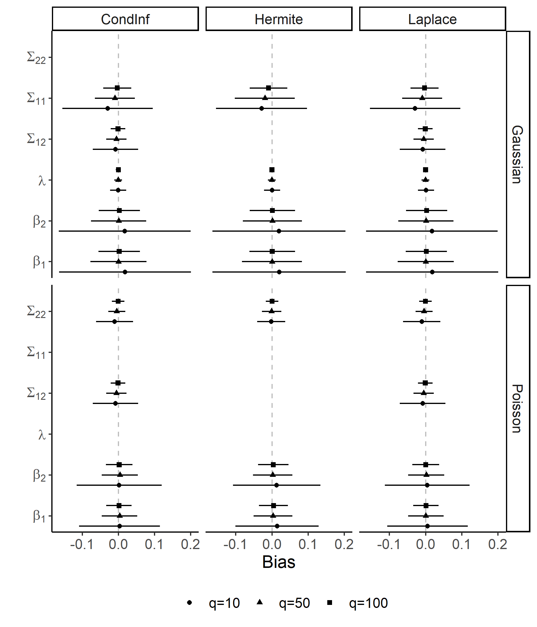
In this section, we present results of two simulation studies illustrating basic properties of the proposed estimation procedure. Moreover, we compare the behaviour of the proposed estimates with two other inference methods: the multivariate Laplace approximation suggested by Breslow & Clayton 1993 (see Appendix A.4 for details) and a Hermite quadrature estimation procedure. Two simulation studies are presented to study the distribution of the estimates when the entries in the covariance matrix are varied, and the bias of the estimated parameters when we increase the numbers of clusters of the random component (and thereby the number of observations). In both simulation studies, we simulate a two dimensional generalised linear mixed model, where $Y_{ij}$ for $i=1,\ldots,n$ and $j=1,2$ denotes the response variables. We follow the notation introduced above and let $\bm{B}_{(1)}$ and $\bm{B}_{(2)}$ denote $q$-dimensional random vectors representing the random components in the model. We assume that $Y_{11},\ldots,Y_{n2}$ are conditionally independent given $\bm{B}_{(1)}$ and $\bm{B}_{(2)}$. Moreover, we assume that given $\bm{B}_{(1)}$ and $\bm{B}_{(2)}$, $Y_{i1}$ and $Y_{i2}$ are conditionally distributed according to a Gaussian and a Poisson distribution, respectively, with conditional expectations given by

where $\bm{\beta}=(\beta_{1},\beta_{2})=(1.90,0.21)$. The Gaussian conditional distribution is assumed to have a variance of $0.5$ which is not varied in the simulations.

We assume that $\bm{B}^{T}=(\bm{B}_{(1)}^{T},\bm{B}_{(2)}^{T})$ is Gaussian distributed with expectation zero and covariance structure given by

where ${B}_{(j)}^{l}$ denotes the $l\footnotesize^{\mbox{th}}\normalsize$ entry in $\bm{B}_{(j)}$ for $j=1,2$, and

with the constant depending on the simulation study. That is,

where $\bm{I}_{m}$ denotes a $m$-dimensional identity matrix.

In the first simulation study, we simulate the above described model for three different covariance matrices, corresponding to three different values of the constant in (15). In that way, we can examine the sensitivity in the normality of the estimates to an increase in the variance. Theorem 2.1 states that under some regularity conditions, the estimated values of $\bm{\beta}$ should be Gaussian distributed when the variance of the random components goes to zero. That is, the lower the constant in (15) is, the closer is the distribution of $\bm{\beta}$ to a Gaussian distribution. In this simulation study, we used the following constants: $c_{1}=1$, $c_{2}=50$ and $c_{3}=100$. In each of the three simulation studies we simulate $500$ datasets and estimate the above described model for each simulation. The results are presented in Figure 1.

In the second simulation study, we fix the covariance matrix of the random components to $\bm{\Sigma}$ defined in (15) with the constant set to one. In this study, we vary the lengths of $\bm{B}_{(1)}$ and $\bm{B}_{(2)}$ between the values $10$, $50$ and $100$, whereas the lengths was fixed to $60$ in the above described simulation study. For each value of $q$ (the length of each vector of random components), we simulate the model $500$ times and estimate the bias and standard errors of the parameters.

References

- (1)
- Agresti (2002) Agresti, A. (2002), Categorical Data Analysis, John Wiley & Sons.
- Barndorff-Nielsen (2014) Barndorff-Nielsen, O. (2014), Information and exponential families: in statistical theory, John Wiley & Sons.
- Breslow & Clayton (1993) Breslow, N. E. & Clayton, D. G. (1993), ‘Approximate inference in generalized linear mixed models’, Journal of the American statistical Association 88(421), 9–25.
- Cordeiro et al. (2021) Cordeiro, G. M., Labouriau, R. & Botter, D. (2021), ‘An introduction to bent jørgensen’s ideas’, Brazilian journal of Probability and Statistics 35(1), 2–20.
- Demidenko (2004) Demidenko, E. (2004), Mixed Models: Theory and Applications (Wiley Series in Probability and Statistics), Wiley-Interscience, USA.
- Fahrmeir & Tutz (2001) Fahrmeir, L. & Tutz, G. (2001), Multivariate Statistical Modelling Based on Generalized Linear Models, Springer-Verlag New York.
- Jørgensen (1987) Jørgensen, B. (1987), ‘Exponential dispersion models’, Journal of the Royal Statistical Society. Series B (Methodological) pp. 127–162.
- Jorgensen (1997) Jorgensen, B. (1997), The theory of dispersion models, CRC Press.
- Jørgensen & Labouriau (2012) Jørgensen, B. & Labouriau, R. (2012), Exponential Families and Theoretical Inference, Vol. 52, 2 edn, Springer.
- Jørgensen et al. (1996) Jørgensen, B., Labouriau, R. & Lundbye-Christensen, S. (1996), ‘Linear growth curve analysis based on exponential dispersion models’, Journal of the Royal Statistical Society. Series B (Methodological) pp. 573–592.
- Labouriau (2020) Labouriau, R. (2020), ‘Construction and extension of dispersion models’. arXiv:2008.05448.
- McCulloch (1997) McCulloch, C. E. (1997), ‘Maximum likelihood algorithms for generalized linear mixed models’, Journal of the American statistical Association 92(437), 162–170.
- McCulloch & Searle (2001) McCulloch, C. & Searle, S. (2001), Generalized, Linear, and Mixed Models, John Wiley & Sons.
- Pelck & Labouriau (2020) Pelck, J. S. & Labouriau, R. (2020), ‘Using multivariate generalised linear mixed models for studying roots development: An example based on minirhizotron observations’. arXiv:2011.00546.
- Pelck et al. (2021b) Pelck, J. S., Luca, A., Holthusen, H., Edelenbos, M. & Labouriau, R. (2021b), Multivariate method for detection of rubbery rot in storage apples by monitoring volatile organic compounds: An example of multivariate generalised linear mixed models. In preparation.
- Pelck et al. (2021a) Pelck, J. S., Maia, R. P., Pinheiro, H. P. & Labouriau, R. (2021a), ‘A multivariate methodology for analysing students’ performance using register data’. arXiv:2102.10565.
- Shanmugam et al. (2021) Shanmugam, S., Hefner, M., Pelck, J., Labouriau, R. & Kristensen, H. (2021), ‘Complementary resource use in intercropped faba bean and cabbage by increased root growth and nitrogen use in organic production’. Submitted.
Appendix A Appendix
A.1 On the identifiability of the family of conditional densities
Here, we show that the family of conditional densities given by (2.1) is not identifiably parametrised by .
Lemma A.1.
For any and any choice of , and , there exist such that .
Proof.
Take arbitrary , and . Note that because, by construction, there is one entry of the allocation vector that is equal to one and the other entries vanish. Assume, without loss of generality, that the first entry of the vector is equal to (i.e., , the fixed effect of the GLMM contains an intercept) so that , where and are the -dimensional vectors obtained by eliminating the first entry of and , respectively. Taking we have that
The proof follows since , and were taken arbitrarily. ∎
A.2 Technical Proofs of the Asymptotic Distribution of the Conditional Inference Based Estimates
In this appendix, we present a sequence of lemmas and propositions that will culminate with the proof of the Theorem 2.1, which establishes consistency and joint asymptotic normality of the proposed estimator of and the predictor of for small values of the variance of the random components.
A.2.1 Regular Inference Functions
We recall the definition of regular inference functions used in this appendix for the easy of the reader (see the details in Jørgensen & Labouriau 2012, Jørgensen & Labouriau 2012, Chapter 4, from which we draw heavily). Consider a parametric family of distributions and a -finite measure defined on a given measurable space . For each , we chose a version of the Radon-Nikodym derivative (with respect to ), denoted by
Definition 1.
A function is said to be a regular inference function when the following conditions are satisfied for all and for .
- (i)
;
- (ii)
The partial derivative exists for -almost every ;
- (iii)
The order of integration and differentiation may be interchanged as follows:
- (iv)
and the matrix
is positive definite;
- (v)
is nonsingular.
Here denoted the component of the vector function
and denotes the gradient operator relative to the vector , defined by
A.2.2 Some Key Lemmas
We denote the sequences of roots of the inference functions and by and respectively, obtained when the number of observations, , increases. Moreover, define and (for each ). Recall, that the inference function for estimating under , is defined by
for all and .
Lemma A.2.
Under the regularity conditions -, the partial inference functions and are unbiased, that is,
for all , and . Moreover, the partial inference functions and , are regular.
We show that is unbiased since the unbiasedness of follows from the same arguments. Take arbitrarily , and . We aim to show that
The regularity conditions ensure that it is allowed to interchange the order of differentiation and integration in the following:
The proof follows since , and are arbitrarily chosen.
The other regularity conditions for the inference functions follow straightforwardly from the assumed regularity conditions i-iv for the GLMM in play. ∎
We introduce some required notation before presenting the next lemma. Define the sensitivity block matrices
and the variability matrices
Using these, we define
Lemma A.3.
The inverse Godambde information for the inference function is the matrix-valued function defined by
with
for all and using the above introduced notation.
The result follows from the formulas in Chapter 4 in Jørgensen & Labouriau 2012 and inversion of block matrices. ∎
Lemma A.4.
Assume the regularity conditions -. Then, for all , and , it is true that
Moreover,
implying that
and
The proof follows from the results in Chapter 4 in Jørgensen & Labouriau 2012, and the fact that and are regular inference functions as a consequence of Lemma A.2. ∎
A.2.3 On the asymptotic variance of under the family
Lemma A.5.
Assume the regularity conditions -. The partial solution of is also a solution to defined in (13), and the unconditionally asymptotic covariance matrices (for converging to infinity and fixed), denoted AV, of and are given by