Vol.0 (20xx) No.0, 000–000
Spectral energy distribution similarity of the local galaxies and the 3.6m selected galaxies from the Spitzer Extended Deep Survey
Abstract
The Spitzer Extended Deep Survey (SEDS) as a deep and wide mid-infrared (MIR) survey project provides a sample of 500000+ sources spreading 1.46 square degree and a depth of 26 AB mag (3). Combining with the previous available data, we build a PSF-matched multi-wavelength photometry catalog from u band to 8m. We fit the SEDS galaxies spectral energy distributions by the local galaxy templates. The results show that the SEDS galaxy can be fitted well, indicating the high redshift galaxy () shares the same templates with the local galaxies. This study would facilitate the further study of the galaxy luminosity and high redshift mass function.
keywords
cosmology: observations — galaxies:high-redshift — galaxies: evolution — galaxies: statistics — infrared: galaxies1 introduction
The mid-infrared (MIR) survey permits an unbiased census of red and blue galaxies. The Spitzer space telescope Infrared Array Camera (Fazio et al. 2004, IRAC, ) can efficiently detect the faint galaxies at redshift about 1 with much shorter exposure time because the galaxy spectral energy distribution (SED) shape peaks in the rest frame near infrared band. The galaxy rest-frame Near-infrared (NIR) band flux is dominated by the old stellar population, which traces the underlying stellar mass (Cowie et al. 1996; Huang et al. 1997). Thus the rest frame NIR selected galaxy sample is equivalent to a mass selected sample (Huang et al. 2013) completed for both the blue and red population. Therefore, a deep IRAC survey would provide us a unique chance to understand the galaxy properties as the stellar population, galaxy color evolution and so on with highly completeness and much wider redshift range.
Galaxy populations are bimodally distributed in color, morphology, metallicity and so on which indicates a divergence galaxy evolution path. The mechanism that governs these observation results is still under debate. This depart phenomenon can be illustrated more clearly in color-magnitude diagram (Baldry et al. 2004; Faber et al. 2007; Schawinski et al. 2014), where the galaxies locate in blue cloud (BC) or red sequence (RS). The blue cloud galaxies are still star-forming while the red sequence galaxies are always full of quiescent galaxies.
Previous IRAC source population was mainly studied to the depth about 23 AB mag or less. The shallow survey as SWIRE (Rowan-Robinson et al. 2005) and Bootes fields (Eisenhardt et al. 2004) have shown the color properties (Rowan-Robinson et al. 2005), redshift distribution (Brodwin et al. 2006; Rowan-Robinson et al. 2008; Rowan-Robinson et al. 2013), galaxy population (Davoodi et al. 2006) and the clustering of the IRAC galaxy (Zeimann et al. 2013, and ref. therein) with wide area. The deep IRAC survey project as the EGS (Barmby et al. 2008), COSMOS (Sanders et al. 2007), HUDF and GOODS-South (Labbé et al. 2005; Labbé et al. 2015; Damen et al. 2011), SPLASH (Capak et al. 2012) revealed us the rest frame K band luminosity function, stellar mass density evolution (Huang et al. 2013), the star formation rate estimation (Barro et al. 2011a; Barro et al. 2011b), star formation history (Steinhardt et al. 2014), high redshift red galaxies (Papovich et al. 2006), lyman break galaxies (Huang et al. 2005; Rigopoulou et al. 2006); optical/NIR dropout galaxies (Yan et al. 2005; Huang et al. 2011; Caputi et al. 2012) and high redshift dusty galaxies (Wang et al. 2016; Wang et al. 2019). IRAC survey deeper than 24 AB mag projects, such as the Spitzer Extended Deep Survey (SEDS) are just beginning to be explored (Ashby et al. 2013; Ashby et al. 2015). In this paper, we aim to study the SEDS source population by comprising the galaxy spectral energy distribution (SED) with the local well-observed galaxies.
The SEDS survey covered in total 1.46 square degree with the 3 depth about 26 AB mag in and bands. The SEDS fields include the Extended Groth Strip (EGS), The Cosmic Evolution Survey (COSMOS), the UKIDSS Ultra-Deep Survey (UDS), the Extended Chandra Deep Field South (ECDFS) and the Hubble Deep Field North (HDFN) region. All the five survey fields have also been covered by many previous optical/NIR survey project. Moreover, Cosmic Assembly Near-infrared Deep Extragalactic Legacy Survey (CANDELS; Gorjian et al. 2008; Koekemoer et al. 2011, PIs: S. Faber, H. Ferguson) project performed a NIR survey within the SEDS region and obtained F120W and F160W band Hubble Space Telescope (HST) WFC3 image up to 27 AB mag with high completeness and spatial resolution. Thus we can derived the SED of the SEDS source from all the available archive data, and investigate the IRAC detected source properties.
To understand the multi-wavelength properties, we also need galaxy templates for the SED fitting. Templates such as the BC03(Bruzual & Charlot 2003) have already shown a great power in describing nearly all the galaxy SEDs (Kriek et al. 2009; da Cunha et al. 2008). However, BC03 only have the stellar spectra with no emission line from ionized gas, and lack of the dust components in MIR(Brodwin et al. 2006; Huang et al. 2013; Huang et al. 2021), and thus do not suitable for fitting our SEDs from u to 8m. Brown et al. 2014 provides 129 galaxy templates that either directly extracted from the observed spectrum or interpolated from Multi-wavelength Analysis of Galaxy Physical Properties code (da Cunha et al. 2008, MAGPHYS,) based on the multi-wavelength SED. The templates show a good coverage of the real galaxy in the color-color diagram like the R-I, B-R diagram and [5.8] - [8.0], [4.5] - [8.0] diagram, which would be more reliable in reflecting and represent the local galaxies SEDs.
The observed 3.6m bright galaxies would include galaxies at a large redshift range, however, high and low redshift galaxies share the same templates is still an assumption. Therefore, in this work, we fit the 3.6m selected sample with local galaxy templates to study whether the high-z galaxy SED have similar templates. The structure of this paper is arranged as follows: Section 2 is data introduction and reduction; in Section 3, we show the main results and then briefly summary in Section 4.
2 Observation and data reduction
2.1 Data for the SEDS region
Ashby et al. 2013has introduced the SEDS data mosaic and the source detection process. All the and mosaic image and coverage map can be obtained from https://www.cfa.harvard.edu/SEDS/.

We collect the available optical, NIR and the and IRAC data to proceed the multi-wavelength photometry. Figure 1 shows the detection rate distribution along the broad band wavelength and the histogram of high S/N source detection band. For the left panel, higher fraction means more complete sample for the multi-band catalog and we can find the shortage always comes in the and band, which is limited by the noise and instruments. The weakness also comes from the NIR band, implying the further requirement of NIR observations. The medium and narrow band photometry in the COSMOS and ECDFS fields would help a lot in populating the galaxy properties (Cardamone et al. 2010). The medium or narrow band data is not take into account in Figure 1. We briefly introduce the data we used for the five SEDS regions as follows.
SEDS-EGS: The image data of SEDS-EGS region we obtained including the u, g, i, z band by the MMT and R band image by the Subaru telescope (Zhao et al. 2009) which cover the whole EGS field. The image data by the MMT and the Subaru telescope have been mosaiced into four separate mosaic images, we perform the photometry on each image and then median the flux for each panel. The HST image is available in HST/ACS F606W, F814W bands11 1 http://www.stsci.edu/~koekemoe/egs/, covered about half area of SEDS-EGS. For the near infrared band, we obtained the Ks band image by Subaru MOIRCS(PIs: Fukugita, Yamada) and the J, H, Ks band image by the WIRCAM Deep Survey (WIRDS) 22 2 http://terapix.iap.fr/rubrique.php?id_rubrique=261(Bielby et al. 2012). Additionally, we use the Subaru telescope Y band data covering the whole EGS map in four pointings (PIs: Newman, Ashby, 2010). Exposure time for the four pointings are 3 minutes, 3 minutes, 3 hours and 9 minutes. The 3 limit magnitudes for 1” aperture are about 24., 23.9, 26.3, 24.7, individually. This Y band data is deducted following the Suprime-Cam pipeline sdfred2. The raw data of Subaru Y band image can be downloaded from the SMOKA database33 3 http://smoka.nao.ac.jp.
In the MIR bands, the , band are fully covered by IRAC EGS survey (Barmby et al. 2008).
Archive catalogs we can make use of in this field include the u, B, g, r, i, z band from CFHTLS, J, Ks or H band from CAHA, Palomar and HST catalog. Figure 1 show the detected source number histogram. sources have been detected at least 5 bands and sources have been detected at least 9 bands. More detail introduction about the EGS image data can be found in Barro et al. 2011a; Barro et al. 2011b; Huang et al. 2013.
SEDS-COSMOS: The SEDS-COSMOS region lies within the 0.3 degree2 of the whole COSMOS field. As a well observed region (Capak et al. 2007; Ilbert et al. 2009; Muzzin et al. 2013; Laigle et al. 2016), COSMOS have been covered by many telescopes in almost all wavelength. We use the u band image by CFHT (McCracken et al. 2010), B, g, V, r, i, z, as well as 12 optical medium bands (IA427, IA464, IA484, IA505, IA527, IA574, IA624, IA679, IA709, IA738, IA767, and IA827) and two narrow bands (NB711, NB816) image by Subaru telescope (Taniguchi et al. 2007; Taniguchi et al. 2015). For the NIR band, we use the image from UltraVista observation in Y, J, H, Ks bands (McCracken et al. 2012). For the MIR band, we use the , data from the S-COSMOS project (Sanders et al. 2007). All the COSMOS image data can be download at http://irsa.ipac.caltech.edu/data/COSMOS/images/ or SEDS website.
Detection band histogram of the SEDS-COSMOS field can be found in Figure 1. The band source rate is about 85% which is caused by the band image overlapping the image about 85%.
SEDS-UDS: The SEDS-UDS region locates in center part of the UDS field (Lawrence et al. 2007; Cirasuolo et al. 2007) with the area about 0.3 degree2. We use the u band image from the CFHT Large Area U-band Deep Survey (Sawicki et al. 2019, CLAUDS) project, the B, V, R, i, z bands from the Subaru telescope SXDS project44 4 http://soaps.nao.ac.jp/SXDS/Public/DR1/index_dr1.html (Furusawa et al. 2008) and the J, H, Ks bands from UKIDSS 55 5 http://www.nottingham.ac.uk/astronomy/UDS/data/dr3.html(Lawrence et al. 2007). The , band IRAC image data can be found in the Spitzer Public Legacy Survey of the UKIDSS Ultra Deep Survey (SpUDS)66 6 http://irsa.ipac.caltech.edu/data/SPITZER/SpUDS/images/irac/.
SEDS-ECDFS: In the SEDS-ECDFS fields region, we use the optical data by ESO U38, U, B, V, R, I band image and 14 Subaru medium bands (IA427, IA445, IA464, IA484, IA505, IA505, IA527, IA550, IA574, IA598, IA624, IA651, IA679, IA709, IA738, IA767, IA797, IA827, IA856) image by MUSYC project77 7 http://www.astro.yale.edu/MUSYC/ (Cardamone et al. 2010). The NIR band image data we used are the J, Ks band by CTIO and H band by ESO NTT. We also use the J, Ks band image data by the Taiwan ECDFS Near-Infrared Survey 88 8 http://www.asiaa.sinica.edu.tw/~bchsieh/TENIS/About.html (Hsieh et al. 2012, TENIS;). The ECDFS field have been covered by the Spitzer IRAC/MUSYC Public Legacy Survey in the Extended Chandra Deep Field South (Damen et al. 2011, SIMPLE;) in band 99 9 http://irsa.ipac.caltech.edu/data/SPITZER/SIMPLE/.
The ECDFS detection band histogram in Figure 1 shows a peak when detection band , which is caused by the optical and NIR region only covers about 70% of the SEDS-ECDFS field and thus there are 30% source have only been covered by the IRAC.
SEDS-HDFN: The optical bands of SEDS-HDFN have been observed by KPNO in the U band, and by Subaru telescope Superime-Cam in the B, V, R, i, z band. The NIR band image data we used are the HK’ band by UH 2.2m telescope 1010 10 http://www.astro.caltech.edu/~capak/hdf/ (Capak et al. 2004) and the Ks band by CFHT WIRCam (Wang et al. 2010). We also take the public catalog by Yang et al. 2014 into account. The band image can be found in the Spitzer Heritage Archive 1111 11 http://sha.ipac.caltech.edu/applications/Spitzer/SHA/.
Optical and NIR band image of SEDS-HDFN field covered about 90%. Therefore, similar as SEDS-ECDFS regions, the histogram of detected band number also shows a little peak for the low band number end in Figure 1.
2.2 PSF-matched photometry
Ashby et al. 2013 provides us a well defined and selected catalog individually. As the and band source are too crowd relative to the image spatial resolution, The source detection method is fitting every source beyond 3 of the image noise by the image PSF, and then iterate the detection with the bright-source-subtracted image. Finally, all the three detection catalogs are combined as the final coordinate catalog. To reduce the contamination of the nearby source in the crowd field, for each IRAC target, all the nearby sources are subtracted with the flux measured by PSF fitting, leaving the only source that we would aperture photometried. The background within the aperture is estimated by the mod pixel value of the annulus. We match the band catalog with the band catalog position. The 2.4” diameter aperture photometry results of and band source are corrected by the PSF growth curve to approach the total flux. Details of the SEDS catalog can be found in (Ashby et al. 2013).
We perform the PSF-matched photometry with the target coordinates from SEDS catalog to the multi-wavelength images. We build the image PSF by stacking the point source image. Then we create and convolve the PSF kernel from each optical and NIR band image to the band PSF by assuming a gaussian shaped PSF in each band. Relation between the of the kernel and PSFs is, where is the kernel we used to convolve the optical and NIR image to the same resolution as band image. We perform the 2.4” diameter aperture photometry on the convolved stamp image, and correct the aperture flux to total flux from the PSF growth curve. Then we calibrate the aperture flux with available catalog, which will give us the photometry results following the same manner as the band.
The PSF width of the , band image is similar to the and image, so we simply perform the aperture photometry without convolution and also corrected by PSF growth curve individually to obtain the total flux.
Uncertainty of photometry can be derived from the standard aperture photometry formula 1212 12 https://wise2.ipac.caltech.edu/staff/fmasci/ApPhotUncert.pdf which contains the CCD gains, pixel exposure time, etc. However, as most of the image data we used are the mosaic image and the information as CCD gains, background counts and coverage map for each pixel and so on are not always provided, and hence unable to derive the Poisson error follow the photometry formula. To estimate our photometry accuracy, we randomly insert 100 fake sources into the image with a known magnitude and then perform the aperture photometry exactly as the way we have done on the real source. The histogram of the (input magnitude - measured magnitude) shows the accuracy and bias of our photometry. Then we interpolate the photometry results with the simulated magnitude v.s. magnitude error relation.

2.3 Star/galaxy separation
There are many color color plot can be used for the Star/Galaxy separation(Huang et al. 1997; Daddi et al. 2004; Barmby et al. 2008; Huang et al. 2013). For the SEDS catalog, the optical band image is deeper and provide more coverage than the NIR band, and thus we plot R - I V.S. R - [3.6] color diagram in Figure 2 with all the five SEDS region catalog to perform the star galaxy separation. Despite the difference for each optical image filter and depth, we can still see the clear separations as two islands and one branch. The two islands mainly consist low and high redshift galaxies separately (Huang et al. 2013) while the branch are formed by the halo K or M star with low metallicity (Guo et al. 2013). We also match the SEDS catalog with the CANDELS catalog and plot the CANDELS STAR_FLAG 0.98 with the red color dots in Figure 2. In this paper, we classify a source as galaxy with , which is shown in solid lines in Figure 2.
2.4 selected catalog completeness: compare with HST CANDELS sample
Each SEDS region has been covered by CANDELS project in the center 200 arcmin2 in F120W, F160W band (Galametz et al. 2013; Guo et al. 2013; Nayyeri et al. 2017; Stefanon et al. 2017; Barro et al. 2019). Facilitating for the HST spatial resolution, CANDELS provide a TFIT catalog (Laidler et al. 2007) by fitting the low resolution band image based on the prior HST source catalog to derive the source flux of multi-wavelength. This method would trace an accuracy photometry for the low resolution band as well as hold the spatial information. We compare the number density for the CANDELS five region and SEDS in Figure 3 right panel with solid points. Assuming the CANDELS catalog is complete down to AB mag, We would find that after recovering the number counts by completeness curve, up to 80% completeness, the number counts density offset between SEDS and CANDELS is less than 10%. We also plot the 50% complete magnitude of and not surprisingly, the number density division turns larger for the lower completeness.
Nevertheless, we should also notice that the number counts given by Ashby et al. 2013 is recovered from the point source simulation. If the completeness is simulated by an extended source, the detection rate would be lower than the point source (Barmby et al. 2008). Hence we re-run the completeness simulation with not only the point source but also the extend source as shown by the Figure 3. We perform the standard “artificial object” method with three kinds of galaxy: elliptical galaxy with “de Vaucouleurs” profile, compose spiral galaxy with half “de Vaucouleurs” profile and half exponential disk (1:1 flux ratio), spiral galaxy with pure exponential disk profile (Huang 1997). All those mocked artificial galaxies are set as axial ratios = 1, effective radii pixel and being convolved with image PSF. The artificial sources are normalized to the AB mag range from 18 to 26 and inserted in the mosaic image, then detected and photometried with the same manner as the real source. In order not to affect the noise of the mosaic image, we input less then 500 artificial source for each run. We consider the object as recovered when the position is within a radius of 1” and the source measured flux is within 80% to 120% of the source input flux. The source detection method we employed here is PSF fitting, hence the artificial point source can be recognised easier, so we can see the source recover rate is lower for the extent source than the point source. For those artificial galaxies, the surface brightness profile of the elliptical galaxy is sharper than the exponential disk profile in the center region, therefore the disk galaxy recover rate is the lowest while the elliptical galaxy is slightly larger than that of the compose spiral galaxy from 22 to 24 AB mag. Although these detection simulations cannot cover all galaxy morphology, we can still expect the real galaxy detection rate would below that of the point source.
Considering the completeness curve of galaxies, we re-plot the number counts density of [3.6]. As the open circles in the right panel of Figure 3, which stand for the source number counts corrected by the extent source completeness curve, we can see the galaxy number counts density is more consistency with that of HST image up to 24 AB mag.


3 Similarility of the local and SEDS galaxy sample: SED fitting


3.1 SED fitting with local galaxy templates
The CANDELS catalog provide the photo-z based on the TFIT photometry result by the template fitting method (Dahlen et al. 2013; Grazian et al. 2015; Song et al. 2016). We match the SEDS galaxy with the CANDELS target to get the phot-z of our SEDS galaxy, and fit the CANDELS-matched SEDS source by the local galaxy templates assuming the CANDELS photo-z can stand for the SEDS target. Since the SEDS catalog, CANDELS phot-z and the local galaxy templates are obtained independently, the fitting results would be an consistent check of the CANDELS phot-z accuracy and the local galaxy templates. We fit the SED from the u band to Ks band. Each SEDS galaxy can be found a galaxy template that gives minimal :
| (1) |
where the , are the observed mag and error of the band X and the is the galaxy template mag measured from the template spectrum. The is the degree of freedom (number of fitting bands). The normalize factor, NF, that minimal the is
| (2) |
Figure 4 shows the reduced of the template fitting results. The left panel of the Figure 4 shows the -[3.6] relation. We also show the histogram for the targets with in red dot line in Fig. 4 left panel. Most of the targets with are the [3.6] brighter than 22 AB mag targets.
Right panel of Figure 4 shows the distribution along the photometric redshift. Several filaments of the redshift shows the cosmology structure. The low redshift sources are also not fitted well with large . Most of the SEDS source locates at redshift about 1 and for the galaxy , the is in the order of 1. Therefore, the local galaxy templates can represent most of the SEDS source. Moreover, the local galaxy templates can represent the SEDS source properties for the redshift larger than 0.5. The large value for the 3.6m bright source indicates that the 129 local galaxy templates are not enough to describe the SEDs. Based on the distribution in Fig. 4, we set as ‘good fit’ in this work, which means our SED can be represented by one local galaxy SED.
The criterion of is based on the histogram in the left panel of Fig. 4. A similar SED fitting work by Huang et al. 2021 fitted the 16m selected galaxy SED by the templates given by Brown+ 2014, and treat targets as outlier. we follow the same criterion as Huang et al. 2021.
However, the similarity of the SED between our targets and the local galaxies may not imply the similarity between the galaxy other properties, such as morphology, stellar mass etc (Huang et al. 2021). The connection between the SED similarity and other galaxy properties will be investigated in an upcoming work.

3.2 SED fitting results in the UVJ diagram
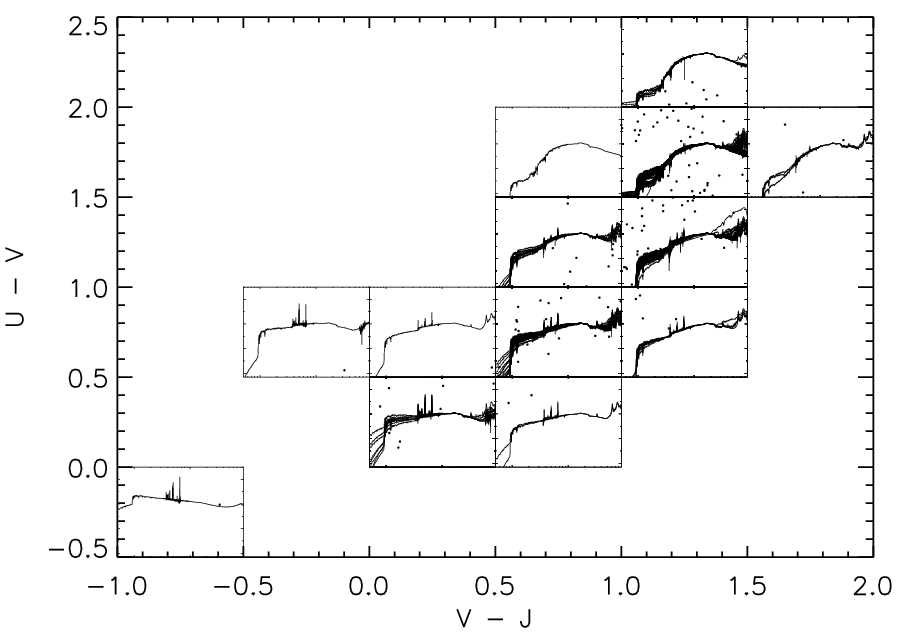
UVJ plot can effectively separate the red, blue and dusty galaxy(Williams et al. 2009; Patel et al. 2012) because the dust extinction and old stellar population are evolving in orthogonal direction. We show the UVJ plot of the templates in Fig. 5 left panel and divide the color-color diagram into grids to show the galaxy population by the location of galaxy in this diagram. Template colors are obtained by performing the photometry with Bessell-U, Bessell-V, Palomar-J band filter on template SEDs.
We derive the absolute mag by the nearest band flux and the K-correction deduced from the best fitting templates and filters. Formulas for the K-correction and absolute mag are given by Hogg et al. 2002. The results is shown in Figure 5 right panel. The red dots in Figure 5 are the U-V, V-J colors measured from the templates.
The fitting results in each UVJ grid is shown in Figure 6. The percentage in each color grid shows the fraction of the source fitting by the templates in the grid. There are in total about 80% SEDS source can be fitted by the local galaxy templates (). This percentage shows the consistency between the local galaxy SED and SEDS multi-wavelength photometry. Nearly 90% blue galaxies and 60% red galaxies can be represented by the local galaxies template, which indicates no difference for the rest frame UV and optical band. The IRAC band data also shows consistency with the rest frame NIR band.
3.3 Examples of the SED fitting
The reduced as a summary of the deviation for every fitting band only reflect the integrated comparison between the data and model. To find the fitting goodness for each band, we overplot the source SED on the best fitting templates with the photometry data. Figure 7 shows some examples of the fitting results. We can see a bump near the [OIII] lines which means the emission lines are commonly existed in the blue galaxies, suggesting the necessity of templates with emission lines(Leja et al. 2017, e.g., ). The emission lines also caused the scatter for the blue galaxy in UVJ diagram (Speagle & Eisenstein 2015; Yuan et al. 2019).
For the blue galaxy example (upper left panel in Fig. 7), UGCA 208, there are in total 995 SEDS sources that minimize the on this template. Most of the SEDS galaxies with locate in redshift 1 (Fig. 4), thus the IRAC band data would be about rest frame NIR. We can find the IRAC data are also recovered by the blue galaxy UGCA 208 template. As we denoted in the upper left panel of the Figure 7, 882 / 995 = 88.6% source can be fitted within . This result shows that the galaxies in redshift 1 are very similar to the local galaxies. The UGCA 208 is an AGN identified from the BPT diagram. From the fitting results, we conclude the AGN continuum is sinking inside the galaxy spectrum. For another local galaxy NGC 3310 (upper right panel in Fig. 7), which have a similar U-V, V-J color as the UGCA 208, is star-forming galaxy due to the BPT criterion. This template can fit 83% source with a with a consistency IRAC radiation.
| 18.75 | 0.236111 | 0.763889 |
| 19.75 | 0.355082 | 0.644918 |
| 20.75 | 0.625544 | 0.374456 |
| 21.75 | 0.803023 | 0.196977 |
| 22.75 | 0.924637 | 0.0753633 |
In the case of the red galaxy NGC 5866 templates, we plot the SEDS source with and all the SEDS sources with minimal fitting on the NGC 5866 templates in the middle panel of Figure 7. Two dots near 7000Åare examples of bad fitting, which may lead to the . Besides this outlier dots, there is no visually difference between the two results. The galaxies with are still consistent with the template.

For the example of NGC 1068, which is an AGN and shows power-law in MIR bands, which is the emission from AGN heated dust (lower right panel in Fig. 7). The NGC 1068 template can also fit 68% SEDS source from the u to Ks band, which means the MIR power-law galaxies SEDs are indistinguishable with a normal galaxies in optical and NIR band. Meanwhile, the SEDS sources well fitted by NGC 1068 template do not follow a similar power-law in MIR, indicating the MIR power-law galaxies are still normal in optical bands (Alonso-Herrero et al. 2006).
For some blue galaxy templates, we find the IRAC flux is brighter than the templates for about 0.5 mag (lower left panel of Fig. 7 and left panel of Fig. 8). We discuss this feature in the next Section. All the templates and the SEDs are shown in the appendix.


3.4 3.6m flux excess in blue galaxies
For the extreme V-J blue galaxies, such as UM 461 in Fig. 7 the IRAC flux, which is about rest-frame J band, is excessing for about 0.5 mag (also see left panel of Fig. 8). Similar excess also shows in the templates UGCA 166, UGCA 219, Mrk 0930, UGC 06850, Mrk 1450, Mrk 0475, all of which are very blue for and . Referring to the UVJ diagram for other surveys (Whitaker et al. 2011; Muzzin et al. 2013), there are very few galaxies bluer than . These galaxies are young, low mass and very active in star formation. Their colors are blue from UV to about 5, then turns red at longer wavelength.
A similar excess phenomenon can be found in fitting the GAMA SEDs data (Taylor et al. 2011). There is a systematically excess in rest frame NIR band flux if only u g r i z band is fitted by stellar population library (SPL) (Taylor et al. 2011, e.g. Fig. 7 & A1 in ) and by a series of analyse, Taylor et al. 2011 conclude that the NIR excess might caused by the NIR data, simple stellar population(SSP) model or the SPL. In our case, as the local galaxy templates can fit the optical and NIR data with consistency IRAC flux except for the six extreme blue galaxies, the offset is more likely not caused by the data. Otherwise there should be an offset for most of the templates.
This rest-frame NIR excess might be caused by the stellar population that exist in blue galaxies. Maraston 2005 stress the importance of the thermally pulsating asymptotic giant branch (TP-AGB) star, which might contribute significantly to the rest-frame NIR luminosity in young galaxies. The follow up work (Maraston et al. 2006) also shows the consistency fitting results of the TP-AGB population, which might also help in alleviating the Age/metallicity degeneracy in the optical bands (Worthey 1994). Due to the position of UM 461 in UVJ diagram, the age of the UM 461 well fitted SEDS sources are about 1 Gyr (Patel et al. 2012, e.g. Figure 1 in). The bands we used for the template fitting are about the rest frame UV to the optical band and thus the minimal method might only catch the main features in optical and miss the accuracy in rest frame NIR band. However, the uncertainty of the stellar population synthesis model is controversy (Maraston et al. 2006; Kriek et al. 2010), and the template we used should include the TP-AGB stars. Maybe the local galaxy templates we used here are still not complete for the blue galaxies. We also fit the SEDS source from u to band and the results are plotted in the Figure 8. Target number with minimal at the template UM 461 decrease from 745 to 469. We can see no rest frame NIR excess in the template fitting from u to m.


4 Summary
In this paper, we investigate the SEDS galaxy population by comparing the SEDS multi-wavelength SED with the local galaxy template. We build multi-wavelength catalog for the SEDS targets. After carefully simulate the completeness, we find that the IRAC number counts is consistent with the CANDELS F160W band selected sample. Our SEDS photometry, the CANDELS phot-z and the local galaxy templates show a consistency with each other. The SEDS galaxies mainly locate at redshift 1, which can be fitted well by the templates from the local galaxies. Consequently, the main evolution is the relative galaxy number counts, not the stellar population. Moreover, this result also confirms the CANDELS photometric redshift for the redshift 1 galaxy is consistent.
As we only fit the galaxy SEDs from u to Ks band, we find a high consistency of MIR radiation between the local galaxy template SEDS galaxy IRAC flux. We also find the low mass galaxy templates do not fit the IRAC flux well and have about 0.5 mag excess. This excess may caused by the poor completeness of the low mass galaxy templates.
In the further work, we will focus on the other properties similarity of the SEDS galaxy SEDs and local galaxy templates. The local templates can also facilitate the further study of the SEDS galaxy photo-z, as well as the luminosity and mass function at high redshift.
Acknowledgements.
The authors are very grateful to the anonymous referee for the helpful report. This work is supported by the National Key R&D Program of China grant 2017YFA0402704 and the National Natural Science Foundation of China, No. 11803044, 11933003. We acknowledge the science research grants from the China Manned Space Project with NO. CMS-CSST-2021-A05. This study makes use of data from AEGIS, a multiwavelength sky survey conducted with the Chandra, GALEX, Hubble, Keck, CFHT, MMT, Subaru, Palomar, Spitzer, VLA, and other telescopes and supported in part by the NSF, NASA, and the STFC. Based in part on data products produced by TERAPIX and the Cambridge Astronomy Survey Unit on behalf of the UltraVISTA consortium.The UKIDSS project is defined in Lawrence, et al (2007). Further details on the UDS can be found in Almaini, et al. (in prep). UKIDSS uses the UKIRT Wide Field Camera (WFCAM; Casali, et al, 2007). The photometric system is described in Hewett, et al (2006), and the calibration is described in Hodgkin, et al. (2009). The pipeline processing and science archive are described in Irwin, et al (in prep) and Hambly, et al (2008).References
- Alonso-Herrero et al. (2006) Alonso-Herrero, A., Pérez-González, P. G., Alexander, D. M., et al. 2006, ApJ, 640, 167
- Ashby et al. (2013) Ashby, M. L. N., Willner, S. P., Fazio, G. G., et al. 2013, ApJ, 769, 80
- Ashby et al. (2015) Ashby, M. L. N., Willner, S. P., Fazio, G. G., et al. 2015, ApJS, 218, 33
- Baldry et al. (2004) Baldry, I. K., Glazebrook, K., Brinkmann, J., et al. 2004, ApJ, 600, 681
- Barmby et al. (2008) Barmby, P., Huang, J. S., Ashby, M. L. N., et al. 2008, ApJS, 177, 431
- Barro et al. (2011a) Barro, G., Pérez-González, P. G., Gallego, J., et al. 2011a, ApJS, 193, 13
- Barro et al. (2011b) Barro, G., Pérez-González, P. G., Gallego, J., et al. 2011b, ApJS, 193, 30
- Barro et al. (2019) Barro, G., Pérez-González, P. G., Cava, A., et al. 2019, ApJS, 243, 22
- Bielby et al. (2012) Bielby, R., Hudelot, P., McCracken, H. J., et al. 2012, A&A, 545, A23
- Brodwin et al. (2006) Brodwin, M., Brown, M. J. I., Ashby, M. L. N., et al. 2006, ApJ, 651, 791
- Brown et al. (2014) Brown, M. J. I., Moustakas, J., Smith, J. D. T., et al. 2014, ApJS, 212, 18
- Bruzual & Charlot (2003) Bruzual, G., & Charlot, S. 2003, MNRAS, 344, 1000
- Capak et al. (2004) Capak, P., Cowie, L. L., Hu, E. M., et al. 2004, AJ, 127, 180
- Capak et al. (2007) Capak, P., Aussel, H., Ajiki, M., et al. 2007, ApJS, 172, 99
- Capak et al. (2012) Capak, P., Aussel, H., Bundy, K., et al. 2012, SPLASH: Spitzer Large Area Survey with Hyper-Suprime-Cam, Spitzer Proposal
- Caputi et al. (2012) Caputi, K. I., Dunlop, J. S., McLure, R. J., et al. 2012, ApJ, 750, L20
- Cardamone et al. (2010) Cardamone, C. N., van Dokkum, P. G., Urry, C. M., et al. 2010, ApJS, 189, 270
- Cirasuolo et al. (2007) Cirasuolo, M., McLure, R. J., Dunlop, J. S., et al. 2007, MNRAS, 380, 585
- Cowie et al. (1996) Cowie, L. L., Songaila, A., Hu, E. M., & Cohen, J. G. 1996, AJ, 112, 839
- da Cunha et al. (2008) da Cunha, E., Charlot, S., & Elbaz, D. 2008, MNRAS, 388, 1595
- da Cunha et al. (2008) da Cunha, E., Charlot, S., & Elbaz, D. 2008, MNRAS, 388, 1595
- Daddi et al. (2004) Daddi, E., Cimatti, A., & Renzini, A. 2004, ApJ, 617, 746
- Dahlen et al. (2013) Dahlen, T., Mobasher, B., & Faber, S. M. 2013, ApJ, 775, 93
- Damen et al. (2011) Damen, M., Labbé, I., van Dokkum, P. G., et al. 2011, ApJ, 727, 1
- Davoodi et al. (2006) Davoodi, P., Oliver, S., Polletta, M. C., et al. 2006, ApJ, 132, 1818
- Eisenhardt et al. (2004) Eisenhardt, P. R., Stern, D., Brodwin, M., et al. 2004, ApJS, 154, 48
- Faber et al. (2007) Faber, S. M., Willmer, C. N. A., Wolf, C., et al. 2007, ApJ, 665, 265
- Fazio et al. (2004) Fazio, G. G., Hora, J. L., Allen, L. E., et al. 2004, ApJS, 154, 10
- Furusawa et al. (2008) Furusawa, H., Kosugi, G., Akiyama, M., et al. 2008, ApJS, 176, 1
- Galametz et al. (2013) Galametz, A., Grazian, A., Fontana, A., et al. 2013, ApJS, 206, 10
- Gorjian et al. (2008) Gorjian, V., Brodwin, M., Kochanek, C. S., et al. 2008, ApJ, 679, 1040
- Grazian et al. (2015) Grazian, A., Fontana, A., Santini, P., Dunlop, J. S., et al. 2015, A&A, 575A, 96G
- Guo et al. (2013) Guo, Y., Ferguson, H. C., Giavalisco, M., et al. 2013, ApJ, 207, 24
- Guo et al. (2013) Guo, Y., Ferguson, H. C., Giavalisco, M., et al. 2013, ApJS, 207, 24
- Hogg et al. (2002) Hogg, D. W., Baldry, I. K., Blanton, M. R., et al. 2002, arXiv:0210394
- Hsieh et al. (2012) Hsieh, B.-C., Wang, W.-H., Hsieh, C.-C., et al. 2012, ApJS, 203, 23
- Huang (1997) Huang, J. 1997, A Wide-Field Near-Infrared and Optical Galaxy Survey, PhD thesis, UNIVERSITY OF HAWAII
- Huang et al. (1997) Huang, J.-S., Cowie, L. L., Gardner, J. P., et al. 1997, ApJ, 476, 12H
- Huang et al. (2005) Huang, J.-S., Rigopoulou, D., Willner, S. P., et al. 2005, ApJ, 634, 137H
- Huang et al. (2011) Huang, J.-S., Zheng, X. Z., Rigopoulou, D., et al. 2011, 742, L13
- Huang et al. (2013) Huang, J. S., Faber, S. M., Willmer, C. N. A., et al. 2013, ApJ, 766, 21
- Huang et al. (2021) Huang, J. S., Dai, Y. S., Willner, S. P., et al. 2021, ApJ, 912, 161
- Ilbert et al. (2009) Ilbert, O., Capak, P., Salvato, M., et al. 2009, ApJ, 690, 1236
- Koekemoer et al. (2011) Koekemoer, A. M., Faber, S. M., Ferguson, H. C., et al. 2011, ApJS, 197, 36
- Kriek et al. (2010) Kriek, M., Labbé, I., Conroy, C., et al. 2010, ApJ, 722, 64
- Kriek et al. (2009) Kriek, M., van Dokkum, P. G., Labbé, I., et al. 2009, ApJ, 700, 221
- Labbé et al. (2005) Labbé, I., Huang, J., Franx, M., et al. 2005, ApJ, 624, 81
- Labbé et al. (2015) Labbé, I., Oesch, P. A., Illingworth, G. D., et al. 2015, ApJ, 221, 23
- Laidler et al. (2007) Laidler, V. G., Papovich, C., Grogin, N. A., et al. 2007, PASP, 119, 1325
- Laigle et al. (2016) Laigle, C., McCracken, H. J., Ilbert, O., et al. 2016, ApJ, 224, 24
- Lawrence et al. (2007) Lawrence, A., Warren, S. J., Almaini, O., et al. 2007, MNRAS, 379, 1599
- Leja et al. (2017) Leja, J., Johnson, B. D., Conroy, C., van Dokkum, P. G., & Byler, N. 2017, ApJ, 837, 170
- Maraston (2005) Maraston, C. 2005, MNRAS, 362, 799
- Maraston et al. (2006) Maraston, C., Daddi, E., Renzini, A., et al. 2006, ApJ, 652, 85
- McCracken et al. (2010) McCracken, H. J., Capak, P., Salvato, M., et al. 2010, ApJ, 708, 202
- McCracken et al. (2012) McCracken, H. J., Milvang-Jensen, B., Dunlop, J., et al. 2012, A&A, 544, 156
- Muzzin et al. (2013) Muzzin, A., Marchesini, D., Stefanon, M., et al. 2013, ApJS, 206, 8
- Nayyeri et al. (2017) Nayyeri, H., Hemmati, S., Mobasher, B., et al. 2017, ApJS, 228, 7
- Papovich et al. (2006) Papovich, C., et al. 2006, New Astronomy Review, 50, 134
- Patel et al. (2012) Patel, S. G., Holden, B. P., Kelson, D. D., et al. 2012, ApJ, 748, 27
- Rigopoulou et al. (2006) Rigopoulou, D., Huang, J., Papovich, C., et al. 2006, ApJ, 648, 81
- Rowan-Robinson et al. (2008) Rowan-Robinson, M., Babbedge, T., Oliver, S., et al. 2008, MNRAS, 386, 697
- Rowan-Robinson et al. (2005) Rowan-Robinson, M., Babbedge, T., Surace, J., et al. 2005, AJ, 129, 1183
- Rowan-Robinson et al. (2013) Rowan-Robinson, M., Gonzalez-Solares, E., Vaccari, M., et al. 2013, MNRAS, 428, 1958R
- Sanders et al. (2007) Sanders, D. B., Salvato, M., Aussel, H., et al. 2007, ApJS, 172, 86
- Sawicki et al. (2019) Sawicki, M., Arnouts, S., Huang, J., et al. 2019, MNRAS, 489, 5202
- Schawinski et al. (2014) Schawinski, K., Urry, C. M., Simmons, B. D., et al. 2014, MNRAS, 440, 889
- Song et al. (2016) Song, M., Finkelstein, S. L., Ashby, M. L. N., et al. 2016, ApJ, 825, 5S
- Speagle & Eisenstein (2015) Speagle, J. S., & Eisenstein, D. J. 2015, arXiv:1510.08073
- Stefanon et al. (2017) Stefanon, M., Yan, H., Mobasher, B., et al. 2017, ApJS, 229, 32
- Steinhardt et al. (2014) Steinhardt, C. L., Speagle, J. S., Capak, P., et al. 2014, ApJ, 791, 25
- Taniguchi et al. (2015) Taniguchi, Y., Kajisawa, M., Kobayashi, M. A. R., et al. 2015, PASJ, 67, 104
- Taniguchi et al. (2007) Taniguchi, Y., Scoville, N., Murayama, T., et al. 2007, ApJS, 172, 9
- Taylor et al. (2011) Taylor, E. N., Hopkins, A. M., Baldry, I. K., et al. 2011, MNRAS, 418, 1587
- Wang et al. (2016) Wang, T., Elbaz, D., Schreiber, C., et al. 2016, ApJ, 816, 84
- Wang et al. (2019) Wang, T., Schreiber, C., Elbaz, D., et al. 2019, Nature, 572, 211
- Wang et al. (2010) Wang, W.-H., Cowie, L. L., Barger, A. J., et al. 2010, ApJS, 187, 251W
- Whitaker et al. (2011) Whitaker, K. E., Labbé, I., van Dokkum, P. G., et al. 2011, ApJ, 735, 86
- Williams et al. (2009) Williams, R. J., Quadri, R. F., Franx, M., et al. 2009, ApJ, 1879, 691
- Worthey (1994) Worthey, G. 1994, ApJS, 95, 107
- Yan et al. (2005) Yan, H., Dickinson, M., Stern, D., et al. 2005, ApJ, 634, 109
- Yang et al. (2014) Yang, G., Xue, Y. Q., Luo, B., et al. 2014, ApJS, 215, 27
- Yuan et al. (2019) Yuan, F.-T., Burgarella, D., Corre, D., et al. 2019, A&A, 631, A123
- Zeimann et al. (2013) Zeimann, G. R., Stanford, S. A., Brodwin, M., et al. 2013, ApJ, 779, 137
- Zhao et al. (2009) Zhao, Y.-H., Huang, J.-S., Ashby, M., et al. 2009, RAA, 9, 1061


