Quantum field-theoretical description of neutrino
oscillations in magnetic field
Vadim Egorov, Igor Volobuev
Skobeltsyn Institute of Nuclear Physics, Moscow State University
119991 Moscow, Russia
Abstract
It is shown that the processes of neutrino oscillations in a magnetic field can be consistently described in the framework of a new quantum field-theoretical approach without use of the neutrino flavor states. It is based on the Feynman diagram technique with a modified distance-dependent propagator, which takes into account the geometry of neutrino oscillation experiments. Processes of neutrino oscillations in a magnetic field, where the neutrinos are detected through the weak charged- and neutral-current interaction, have been studied and numerical calculations have been carried out for some specific examples. Implications for the solar neutrinos are briefly discussed, and formulas for the asymptotic values of the normalized probability of solar neutrino oscillation processes are derived, which coincide with the observable ratio of the measurable neutrino flux to that predicted by the standard solar model.
1 Introduction
The Standard Model (SM) allows one to describe, with high accuracy, a great amount of various elementary particle interaction processes in the framework of the S-matrix formalism and Feynman diagram technique. However, there is a belief that it cannot describe the phenomena of neutral kaon and neutrino oscillations, the latter being under intense theoretical and experimental investigation nowadays. The standard way to describe the phenomenon is the quantum-mechanical approach in terms of plane waves [1, 2, 3, 4]. Although being straightforward, it is believed to be inconsistent, because the production of the neutrino flavor states is described within the SM (which is a gauge field theory), whereas their evolution is described within quantum mechanics. Such a description seems to be eclectic, since quantum field theory includes quantum mechanics as an indispensable part and must be able to describe all quantum phenomena. Moreover, the production of states without definite mass leads to violation of energy-momentum conservation [5, 6, 7, 8]. This problem is supposedly solved in the framework of the quantum-mechanical approach it terms of wave packets [3, 9], although this description turns out to be very bulky. Thus, the construction of a consistent and convenient description of neutrino oscillations within quantum field theory is of current interest.
The first attempt to describe neutrino oscillations in the framework of quantum field theory was made back in 1982 in paper [10]. In this paper, within the standard perturbative S-matrix formalism, it was assumed that virtual neutrino mass eigenstates were produced and detected in the charged-current interactions with nuclei. The matrix elements of the charged weak hadron current between the initial and final states of the nuclei were approximated by delta functions of their positions separated by a fixed distance, whereas all the incoming and outgoing leptons were described by plane waves. This approximation fixed the distance between the production and detection points of the neutrinos and, in the momentum representation, resulted in the appearance of distance-dependent neutrino propagators. Hence, neutrino oscillations were regarded as interference of the amplitudes of processes mediated by different neutrino mass eigenstates. In the subsequent studies the delta functions, which seemed to be a rather too rough approximation and formally contradicted the S-matrix formalism, were replaced by localized wave packets for describing the states of the nuclei [5, 6, 7, 11]. However, the calculations in the framework of this approach turned out to be very bulky and complicated. The reason is that the standard perturbative formalism of S-matrix is not suitable for describing processes taking place at finite space and time intervals.
It is a common knowledge that the presence of external fields and matter affects neutrino oscillations [3]. The influence of magnetic fields on neutrino oscillations, as well as its possible implications for the solar neutrino problem were repeatedly considered in the framework of the standard quantum-mechanical description based on the use of the neutrino flavor states in papers [12, 13, 14, 15, 16, 17, 18]. However, up to now, there were no papers dealing with the description of neutrino oscillations in external fields and matter within quantum field theory without use of the flavor states. In the present paper, we develop such a quantum field-theoretical description of neutrino oscillations in a magnetic field. Our approach makes use of a modified perturbative formalism adapted for describing processes passing at finite space and time intervals [19, 20, 21, 22, 23]. The formalism is based on the Feynman diagram technique in the coordinate representation supplemented with modified rules of passing to the momentum representation. The latter reflect the geometry of neutrino oscillation experiments and lead to the Feynman propagator of virtual neutrino mass eigenstates in the momentum representation being modified. Namely, a distance-dependent propagator of neutrino mass eigenstates in the momentum representation arises, while the rest of the Feynman rules in this representation are kept intact. The description in terms of plane waves allows one to avoid cumbersome calculations, while catching the essence of the phenomenon.
In describing neutrino oscillations in a magnetic field, we assume that neutrinos are produced and detected through the charged- and neutral-current interaction with nuclei and electrons in the absence of field, but the propagation of the particles occurs in a region of magnetic field. In Section 2 we give a brief review of the main ideas of the approach. In Section 3 we apply the formalism to the case of neutrino oscillation in a magnetic field, deriving the oscillation probability. In Section 4 we consider specific examples with solar neutrinos, namely neutrino production in decay or electron capture by and detection by Ga-Ge or Cherenkov detectors, and derive useful formulas for the asymptotic values of the normalized probability of solar neutrino oscillation processes, which coincide with the observable ratio of the measurable neutrino flux to that predicted by the standard solar model.
2 Basics of the approach
First, we note that neutrino oscillation experiments are characterized by a specific geometry, where the distance between a neutrino source and a detector is much larger than their sizes. For this reason one can consider the source and detector to be pointlike and describe the oscillation process by just one parameter of geometric origin: the distance between the centers of the source and detector. Moreover, one can use the one-dimensional approximation, where the neutrino momenta are directed along the line connecting the centers, which is usually called the plane wave approximation in the standard quantum-mechanical approach [3].
In what follows we use the one-dimensional approximation. Also, we work in the framework of the minimal extension of the Standard Model by the right neutrino singlets. The interaction Lagrangian of the leptons takes the form
| (1) |
where denotes the field of the charged lepton of the th generation, is the PMNS-matrix, stands for the field of the neutrino state with definite mass , and is the Weinberg angle.
Let us first recall the basics of the approach and consider the case of neutrino oscillations in vacuum. To this end, we consider a process, where a neutrino is produced and detected through the charged-current interaction with nuclei. In the lowest order of perturbation theory the process is described by the following diagram:
![[Uncaptioned image]](2107.11570v2/diag1.png)
The points of production and detection are supposed to be separated by a fixed macroscopic distance along a unit vector . The intermediate virtual neutrino mass eigenstate is described by the Feynman propagator in the coordinate representation. The amplitude corresponding to the diagram must be summed over all the three neutrino mass eigenstates, .
The initial and final nuclei and particles are assumed to be described by plane waves. Their 4-momenta are denoted as it is shown in the diagram: , , correspond to the positron, electron and intermediate virtual neutrino, respectively. The filled circles in the diagram represent the matrix elements of the weak charged hadron current between the states of initial nuclei 1 and 2 and final nuclei and :
| (3) |
the nuclei 4-momenta being denoted by , .
The amplitude of the process in the coordinate representation can be constructed using the Feynman rules formulated, for example, in textbook [24]. The passing to the momentum representation is performed by integrating the amplitude with respect to and over Minkowski space. However, such a straightforward integration would result in losing the information about the space-time interval between the production and detection events. Thus, in order to be able to describe processes passing at finite space and time interval one has to fix somehow the distance between the neutrino production and detection points. To this end, in paper [10] the matrix elements of hadron currents (3) in the coordinate representation were assumed to be proportional to the delta functions with fixed, which, in the approximation of Fermi’s interaction, gave the desired result.
In our approach, instead of fixing the positions of the initial and final nuclei, we just fix the distance between the interaction points along the unit vector directed from the source to the detector by introducing the delta function into the integrand, which gives a generalization of the standard perturbative formalism to the case of processes passing at finite distances.
The introduction of the delta function is formally equivalent to replacing the standard Feynman propagator of the neutrino mass eigenstate in the coordinate representation by . The Fourier transform of this expression was called in paper [19] the distance-dependent propagator of the neutrino mass eigenstate in the momentum representation:
| (4) |
This integral can be evaluated exactly:
| (5) |
where .
According to the Grimus-Stockinger theorem [6]
the virtual particles propagating over macroscopic distances are
almost on the mass shell, and for the momenta satisfying
the distance-dependent propagator can be brought to the simple
form
| (6) |
In particular, this approximation is always valid for the neutrino momenta directed along the vector , which are the only momenta needed for calculating the amplitudes.
Distance-dependent propagator (6) differs from the one found in paper [10]: there the propagator is the projection operator multiplied by a spherical wave, whereas in our case this operator is multiplied by the exponential similar to that appearing in the standard plane wave approximation. It is also necessary to note that a distance-dependent propagator very similar to ours has been obtained in recent paper [25] within a path integral approach.
Finally, using expression (6) instead of the usual Feynman propagator for constructing the amplitude in the momentum representation allows one to consistently describe neutrino oscillations in vacuum [20, 21, 22, 23]. It is worth noting that in this case one can also use the time-dependent propagator, which is obtained by fixing the time interval between the neutrino production and detection events. This is due to the fact that, for the neutrinos almost on the mass shell, the space and time intervals are related by the standard formula
| (7) |
However, this relation is no longer true for neutrinos in an external field, and one has to use distance-dependent propagator (6) in this case.
3 Neutrino oscillations in a magnetic field
Now let us turn a background electromagnetic field on. Neutrinos are able to interact with it through quantum loops, which provides the neutrino with, among others, anomalous dipole magnetic moment. We will take it into account but neglect the transition moments, which are usually assumed to be much smaller. This means that the equations of motion for different neutrino mass eigenstates are not coupled. Thus, the equation of motion of a neutrino mass eigenstate in an external electromagnetic field takes the form
| (8) |
where the magnetic moment of the th neutrino mass eigenstate, proportional to its mass, is and . In the Standard Model, the parameter , which gives, for the experimentally allowed neutrino masses, the neutrino magnetic moments at least 10 orders of magnitude smaller than the Bohr magneton, but they may be much larger in SM extensions.
For a homogeneous electromagnetic field, Green’s function of equation (8) in the momentum representation reads
| (9) |
Here , .
First, we consider a homogeneous magnetic field : , . Then the neutrino dispersion relation following from the denominator of Green’s function (9),
| (10) |
where denotes the component of the magnetic field transverse to the direction of neutrino propagation , coincides, mutatis mutandis, with the dispersion relation for the neutron in a magnetic field, which was first derived in paper [26] and recently reproduced within the standard approach in paper [17] for the neutrinos.
Since the neutrino magnetic moment is extremely small, , we neglect the terms of order 2 and higher in . Substituting the Green’s function in the coordinate representation in definition (4) of the distance-dependent propagator, taking the neutrino momentum to be parallel to and neglecting also the neutrino masses everywhere except in the exponential, we arrive at the distance-dependent propagator of the neutrino mass eigenstate in a homogeneous magnetic field in the momentum representation:
| (11) |
Here , we suppose , and
| (12) |
the square brackets denoting the vector product. Comparing expressions (11) and (6) one can conclude that, in the magnetic field, each neutrino mass eigenstate splits into two states corresponding to two possible spin orientations and energies. This effect is in full agreement with the quantum-mechanical expectations. The numerators in the exponents, , measure the deviation of the virtual neutrinos from the mass shell, which is consistent with dispersion relation (10) in our approximation.
We see that the distance-dependent propagator essentially depends only on the transverse component of a magnetic field. In what follows, we will neglect the longitudinal component of the field and assume the magnetic field to be transverse. Further, propagator (11) has been derived for the case of a constant homogeneous magnetic field. Nevertheless, it can be used for the transverse magnetic field, the magnitude of which varies along the neutrino path adiabatically, i.e., if the condition
| (13) |
is fulfilled, where is the characteristic size of the field region and is the largest neutrino mass. This condition refines the adiabaticity condition for the magnetic field introduced earlier in paper [15]. It takes into account the neutrino magnetic moments, the size of the field region and guarantees that the term in the exponential can be considered to be constant along the path. However, since now the magnetic field varies along the path, the field in formula (11) should be replaced by the mean field
| (14) |
Now we will use distance-dependent propagator (11) with these amendments to calculate the probability of an actual process. Let us first consider a process analogous to the one described by diagram (2), where the neutrinos are produced and detected in the absence of field, but propagate through a region of magnetic field (for which the assumptions above are true). In what follows we will work in the approximation of Fermi’s interaction. Then the amplitude of the process in the momentum representation, where the distance is fixed and equals , looks as follows:
| (15) |
Here we omit fermion polarization indices for brevity; the notations for the momenta are the same as in diagram (2) explained in the paragraph above formula (3). Again, neutrino masses are neglected everywhere, except in the exponential.
The squared modulus of the amplitude (15), averaged over the polarizations of the incoming nuclei and summed over the polarizations of the outgoing particles and nuclei (the operation of averaging and summation is denoted by the angle brackets), factorizes in the approximation of zero neutrino masses. The latter means that we also neglect the terms proportional to , which, due to the Grimus-Stockinger theorem [6], is of the order of neutrino masses squared. In (15), the terms containing the vector vanish, and we arrive at the result
| (16) |
where
| (17) |
is the squared modulus of the amplitude of the production process;
| (18) |
is the squared modulus of the amplitude of the detection process;
| (19) |
are the nuclear tensors characterizing the interaction of nuclei 1, and 2, with the leptons, their symmetric parts being real and the anti-symmetric ones being imaginary;
| (20) |
is the neutrino oscillation probability depending on the neutrino momentum , is the distance between the source and detector and denotes the mean value of the transverse magnetic field; we also introduce the notations similar to the usual ones :
| (21) |
In the case of two neutrino flavors formula (20) is consistent with the ones derived in papers [17, 18] for a homogeneous magnetic field, although it looks different.
We note that, since the neutrinos are produced and detected in the absence of magnetic field and the field is transverse to the neutrino path, the energy and momentum are conserved in the process under consideration. Following the prescription formulated in papers [20, 21, 22], in order to find the probability of the process, before integrating over the phase volume of the final particles, one must multiply expression (16) not only by the delta function of energy-momentum conservation, but also by a delta function, which would guarantee that the momentum of the intermediate neutrinos is directed along the vector . Since we have calculated the squared modulus of the amplitude in the approximation of massless neutrinos, it is natural to calculate the probability in the same approximation, i.e., to choose . A special value of satisfying these conditions will be denoted by , where is directed from the source to the detector and .
Thus, we multiply the squared modulus of the amplitude by the delta function of energy-momentum conservation and also by the delta function , as well as substitute instead of everywhere in (16) [20]. In so doing, we fix the momentum of the intermediate neutrinos, whose direction is determined by the source-detector relative position, and, after the integration over the phase volume, find the differential probability of the process with a definite neutrino momentum. Since the experimental situation determines only the direction of neutrino momentum, but not its magnitude, we must also integrate with respect to over the admissible values. The final probability of the process under consideration reads:
| (22) |
Here
| (23) |
is the differential probability of the decay of nucleus 1 into nucleus , positron and a massless fermion with momentum , which coincides with the sum of differential probabilities of the decay of nucleus 1 into nucleus , positron and all three neutrino mass eigenstates;
| (24) |
is the probability of the scattering process of the massless fermion and nucleus 2 with the production of nucleus and an electron, which coincides with the sum of the probabilities of the scattering processes of all three neutrino mass eigenstates and nucleus 2. The lower limit of integration is determined by the threshold of the registration process and the upper one is determined by the energy-momentum conservation in the production vertex. In what follows, we assume the initial nuclei 1 and 2 to be at rest and put their momenta , equal to zero, then the integration limits are given by [27]
| (25) |
where , , are the nuclear masses and is the electron mass. In the next section we will apply formula (22) to specific neutrino oscillation processes.
It is easy to verify that one arrives at an expression of the same form as (22), if the production process is not a nuclear decay but electron capture:
| (26) |
The only difference is that the differential decay probability (23) must be replaced by the differential scattering probability. Oscillating factor (20) does not change. However, since the reaction has only two particles in the final state, the magnitudes of the momenta are already fixed by energy-momentum conservation. Hence, the differential probability for reaction (26) is singular, and the integration with respect to neutrino momentum magnitude leads to
| (27) |
where is the neutrino momentum magnitude selected by the energy-momentum conservation in the production process and is the differential probability of production of the neutrino moving in the direction of the detector. Since the initial particles always have a momentum distribution, one must average probability (27) over the momenta of these particles.
In the same way we can consider a process, where the neutrino is detected through both the charged- and neutral-current interactions with an electron. The process is described by the diagrams
![[Uncaptioned image]](2107.11570v2/diag2.png)
.
The amplitude corresponding to diagram (29) should be summed over the type of the intermediate neutrino mass eigenstate, because all of them contribute. Since only the final electron is detected in the experiment, the probability of the process with th neutrino mass eigenstate in the final state should be summed over to give the probability of registering an electron.
In order to use the foregoing formulas without redefinitions, we retain the previous notations for particles’ 4-momenta and nuclear values. Besides, we introduce the missing notations and for the 4-momenta of the incoming electron and outgoing neutrino , respectively.
Using the approximation of Fermi’s interaction and distance-dependent propagator (11), keeping the neutrino masses only in the exponential, one can write down the amplitude corresponding to neutral-current diagram (28) in the momentum representation as follows:
| (30) |
The amplitude corresponding to charged-current diagram (29) summed over the index reads
| (31) |
The squared modulus of the total amplitude , averaged and summed over particles’ polarizations, factorizes in the approximation . Following the procedure described above and summing the differential probability over the final neutrino type , we arrive at the probability of detecting an electron in the process at hand:
| (32) |
Here the differential production probability is given by (23) and the total detection probability , which is the sum of the detection probabilities for each neutrino mass eigenstate in the final state, reads
| (33) |
where
| (34) |
| (35) |
Here is the maximum kinetic energy of the final electron in the detection process, determined by energy-momentum conservation, and is the minimum kinetic energy of the electron accessible for registrations by a specific detector. The lower integration limit in (32) is connected with by a relation similar to (35), resolving which we get
| (36) |
It is easy to verify that the detection probability (33) is expressed through the oscillating factor (20) and the Standard Model neutrino scattering probabilities and , calculated for the same values of and , by the relation
| (37) |
which differs from the standard one in vacuum by an extra field-dependent oscillating factor taking into account the neutrino spin rotation.
4 Specific examples
Let us discuss some examples, where neutrinos are produced in the decay of
| (38) |
or in the electron capture reaction
| (39) |
and detected by a gallium-germanium detector in the reaction
| (40) |
Both reactions contribute to the solar neutrino flux, the first reaction having a wide energy spectrum and the second one producing almost monoenergetic neutrinos.
We start with the -source. Nuclear reactions (38), (40) are allowed transitions [28], which means that we can neglect the nucleon positions and momenta and consider the interaction or decay of a nucleon as if it were at rest. Thus, neglecting the dependence of the nuclear form-factors on the momentum transfer [28] and also neglecting the possible contribution of the excited states of the final nuclei, one can approximate the product of the differential probability of neutrino production and the probability of neutrino detection by the function
| (41) |
Here is a constant, the explicit form of which is unimportant for us, because we will normalize the probability (22) so that it equals unity at the point ; and are the same as the integration limits in (22), determined by (25). For the production and detection processes under consideration we have:
| (42) |
Below the following values of the mixing angles are used [29]:
| (43) |
Let the constant take the value predicted by the Standard Model, . Taking into account the experimental restrictions for the masses of the normally ordered neutrinos [29], which is the most likely scenario,
| (44) |
and the cosmological limit [30]
| (45) |
we first take one set of masses,
| (46) |
and then the second one,
| (47) |
The results of numerical integration of formula (22) in the case of homogeneous magnetic field with these parameters for the two sets of masses, in the absence of external magnetic field and for its transverse values , , G are presented in Fig. 1.


Such huge magnitudes of the magnetic field, close to the magnetism limit of neutron stars G, are taken just for an illustration, in order to show both the momentum-dependent and field-dependent oscillations in one picture. As it was discussed in [23], the momentum-dependent oscillations fade out at a rather short distance from the source due to the presence of the neutrino momentum spread, and at larger distances only the field-dependent oscillations are basically left.
Now let us consider a source, where reaction (39), , takes place. This reaction also belongs to the allowed transitions, and one can neglect nuclear form-factors in calculating the matrix elements. In the non-relativistic approximation the squared modulus of the production amplitude, averaged and summed over the polarizations of the nuclei and particles, can be written as [31]
| (48) |
where are constants, is the initial electron energy, is the final neutrino energy and , are the electron and neutrino velocities, respectively. Reaction (39), having a two-particle final state, produces neutrinos with a fixed energy, when the initial particles have definite energies. The neutrino energy has only a thermal broadening due to the spread in the energies of the initial particles. Since the electron mass is 4 orders of magnitude smaller then the nucleus mass, it is the electron energy spread that mainly contributes to the neutrino energy broadening. Taking the plasma temperature to be K, as in the center of the Sun, which is consistent with the non-relativistic approximation, we average probability (27) with the Maxwell-Boltzmann distribution for the initial electron momentum. As a result, the term with the velocities vanishes, and, neglecting the exited states of nucleus, we arrive at the expression
| (49) |
where keV is the reaction energy release (the neutrino mass is neglected), for a Ga-Ge detector is presented in (42), is the neutrino momentum magnitude and is a constant. Performing the numerical integration in the latter formula for two sets of masses (46)–(47) and a Ga-Ge detector, one arrives at the results depicted in Fig. 2.


We see, once again, that the narrower neutrino momentum distribution leads to larger coherence lengths of the momentum-dependent oscillations. Namely, in the case of source of temperature K the coherence length turns out to be about 10 000 km. We do not present the corresponding figure, because the oscillations actually merge into a band on this scale. The curves in Fig. 2 b) resemble those obtained in [18] for the spin-flavor oscillations of monoenergetic neutrinos in homogeneous magnetic field.
Borexino [32] and GEMMA [33] experiments restrict the neutrino magnetic moment from above by the value about , where is the Bohr magneton. This bound is 10 orders of magnitude larger than the value, predicted with the Standard Model , which allows 10 orders of magnitude weaker magnetic field for the same effect.
The results depicted in Figs. 1, 2 refer to the case of a homogeneous magnetic field present along the entire neutrino path. If the neutrinos travel in magnetic field only a part of the path, for fairly large values of , where the momentum-dependent oscillations fade out, the normalized probabilities of all processes are defined only by the magnetic field and go to the asymptotic value
| (50) |
where is the asymptotic value in vacuum, is the phase accumulated by the neutrino mass eigenstate on its path and is the field region with respect to coordinate along the neutrino trajectory.
Let us consider, for example, the solar neutrinos, which are produced in the solar core. As we have shown, even for monoenergetic neutrino sources the coherence length is of the order of 10 000 km. Therefore, when the neutrinos come to the convective zone, all the momentum-dependent oscillations fade out, and only the oscillations due to the solar magnetic field present in this zone remain. These oscillations for , i.e., near the upper limit set by the Borexino and GEMMA experiments [32, 33], the solar magnetic field G used in paper [15], and the first mass set (46) are shown in Fig. 4, where the asymptotic value is given by
| (51) |
with and km. We note that, for the neutrino energy above 200 keV, the size of the field region and the chosen value of the neutrino magnetic moment, adiabaticity condition (13) is fulfilled with a great accuracy. Since the thickness of the solar convective zone is fixed and the product varies depending on the model, it is useful to plot the asymptotic value of the normalized probability as a function of this product, which is shown in Fig. 4 (again, the first neutrino mass set is chosen).

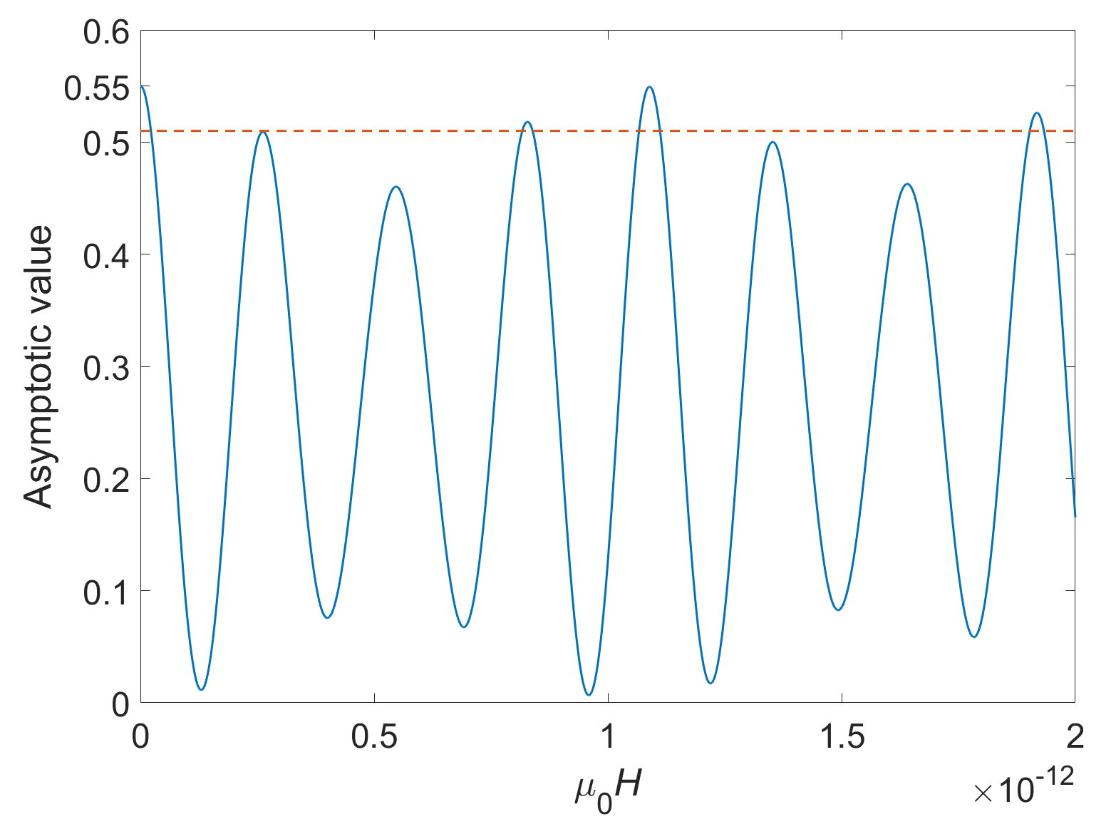
The normalized probability discussed in this paper can be considered as the ratio of the number of neutrinos detected in the presence of oscillations to the number of neutrinos that would have been detected in the absence of oscillations. For the processes with only charged-current interaction its asymptotic value does not depend on the production and detection processes, and for this reason it gives a theoretical prediction for the ratio of the flux of solar neutrinos measured in an experiment with a Ga-Ge (or Cl-Ar) detector to that predicted by the standard solar model. This ratio for the GALLEX + GNO experiments is and for the SAGE experiment [34], which is well consistent with the curve in Fig. 4. We see that there are many values of giving the asymptotic value above the lower experimental limit (dotted line). This means that, if we obtain an experimental value of the neutrino magnetic moments, we will be able to obtain restrictions on the solar magnetic field from the solar neutrino experiments, and vice versa.
In the case of neutrino detection through both charged- and neutral-current interaction the situation is different, because, as it is clearly seen in formula (37), the oscillating factor does not factorize. For this reason the asymptotic value of the normalized probability depends not only on the production process, but also on the energy range, in which the neutrinos are detected. Here we consider the same production processes, the decay and the electron capture by , and the detection by a Cherenkov detector, which is capable of measuring the neutrino energy.
For decay (38), neglecting the dependence of the nuclear form-factors on the momentum transfer, the differential probability of neutrino production can again be approximated by the function
| (52) |
where the maximum neutrino momentum keV. We take keV, which corresponds to a water-based Cherenkov detector. The results of numerical integration for the two neutrino mass sets are depicted in Fig. 5.


The asymptotic values for the oscillation processes with neutral current can be found as follows. Substituting the asymptotic value of (20) into formula (32) for the probability and using the explicit form of (33), we get the asymptotic value of the normalized probability for such processes in the form
| (53) |
where are the phases defined in Eq. (50) and the coefficient is given by
| (54) |
being the scattering probability of a massless neutrino flavor state at an electron, calculated within the framework of the Standard Model. The term with takes into account the contribution of the neutral current. Numerical evaluation of for the neutrino production in the decay in our approximation gives . Using the explicit form of , one can estimate in the interval as .
Finally, let us consider production reaction (39) of electron capture by . Similar to the case of only the charged-current interaction, averaging over the electron momentum distribution in the source, we get the process probability in the form
| (55) |
Assuming the plasma temperature to be K and performing the numerical integration, we obtain the plots presented in Fig. 6.


For this process with the solar neutrinos the coherence length is also of the order of tens of thousand kilometers, and the asymptotic value of the normalized probability is given by the same expression (53), but the coefficient is calculated with the neutrino production probability in the electron capture by . The numerical integration gives , which corresponds to the asymptotic value in vacuum . The ratio of the neutrino flux measured by the Borexino collaboration to that predicted for by the standard solar model is [35]. This is again in a good agreement with our theoretical value and leaves room for a contribution from the solar magnetic field, which is always negative.
5 Conclusion
In the present paper we have shown that it is possible to give a consistent quantum field-theoretical description of neutrino oscillations in a magnetic field in the Standard Model minimally extended by the right neutrino singlets without use of the neutrino flavor states. The description is performed in terms of plane waves and is based on the Feynman diagram technique in the coordinate representation supplemented with modified rules of passing to the momentum representation. These rules reflect the experimental setting and give rise to the distance-dependent propagators of neutrino mass eigenstates. The distance-dependent propagators in a magnetic field are explicitly calculated and found to split into the sum of two terms corresponding to two possible neutrino spin orientations and energies.
Processes of neutrino oscillation have been considered, where the neutrinos are produced and detected through the charged- and neutral-current weak interactions with nuclei and electrons in the absence of magnetic field, but the propagation of the neutrinos takes place in a region of magnetic field. Formulas for the probabilities of the oscillation processes have been derived and an agreement with the results obtained in the standard quantum-mechanical description is shown.
An important new result derived within the framework of the approach is formulas (50) and (53) for the asymptotic values of the normalized probability of processes, where neutrinos are detected through the interaction with nuclei or electrons. For a particular process, this value is the observable ratio of the measurable neutrino flux to that predicted by the standard solar model. These formulas can be immediately compared with the experimental data. For the neutrino detection through the interaction with electrons, also limits on the neutral current contribution to the asymptotic value are set.
The neutrino production in the solar core in decay and electron capture by and detection by Ga-Ge and Cherenkov detectors has been studied. Numerical computations of the normalized probabilities of these processes have been performed and the results have been found to be in a good agreement with the experimental data.
The advantages of the approach are the technical simplicity and physical transparency. It makes use of only the standard tools of perturbative quantum field theory and does not need wave packets and the neutrino flavor states. In fact, we have shown that the Standard Model extended by the right neutrinos is capable of describing not only scattering processes, but also quantum processes passing at finite space and time intervals, like particle oscillations, in the framework of the standard Feynman diagram technique and the modified perturbative formalism.
Finally, we have to note that we have not touched upon the problem of neutrino oscillations in matter and have chosen the examples of the production and detection processes in the energy range, where the influence of oscillations in matter is expected to be weak. A quantum field-theoretical description of oscillations in matter can be developed along the lines set forth in the present paper, although the problem is rather complicated, because one has to invert analytically a 1212 matrix to find Green’s function of neutrino mass eigenstates in matter. Such a description is rigorous and very different from the standard one. Hence the results may also differ. This is a matter of a special investigation.
Acknowledgments
The authors are grateful to E. Boos, A. Lobanov, A. Pukhov and Yu. Tchuvilsky for interesting and useful discussions. Special thanks are due to M. Smolyakov for reading the manuscript. Analytical calculations of the amplitudes have been carried out with the help of the CompHEP and Reduce packages. The work of V. Egorov was supported by the Foundation for the Advancement of Theoretical Physics and Mathematics “BASIS”.
References
- [1] B. Pontecorvo, Mesonium and anti-mesonium, Sov. Phys. JETP 6, 429 (1957) [Zh. Eksp. Teor. Fiz. 33, 549 (1957)].
- [2] V. N. Gribov and B. Pontecorvo, Neutrino astronomy and lepton charge, Phys. Lett. B 28, 493 (1969).
- [3] C. Giunti and C. W. Kim, Fundamentals of Neutrino Physics and Astrophysics (Oxford University Press, Oxford, 2007).
- [4] S. Bilenky, Introduction to the physics of massive and mixed neutrinos, Lect. Notes Phys. 817, 1 (2010).
- [5] C. Giunti, C. W. Kim, J. A. Lee and U. W. Lee, On the treatment of neutrino oscillations without resort to weak eigenstates, Phys. Rev. D 48, 4310 (1993).
- [6] W. Grimus and P. Stockinger, Real oscillations of virtual neutrinos, Phys. Rev. D 54, 3414 (1996).
- [7] M. Beuthe, Oscillations of neutrinos and mesons in quantum field theory, Phys. Rept. 375, 105 (2003).
- [8] A. G. Cohen, S. L. Glashow and Z. Ligeti, Disentangling Neutrino Oscillations, Phys. Lett. B 678, 191 (2009).
- [9] B. Kayser, On the quantum mechanics of neutrino oscillation, Phys. Rev. D 24, 110 (1981).
- [10] I. Yu. Kobzarev, B. V. Martemyanov, L. B. Okun and M. G. Shchepkin, Sum rules for neutrino oscillations, Sov. J. Nucl. Phys. 35, 708 (1982).
- [11] W. Grimus, J. Phys. G 47 (2020) no.8, 085004
- [12] A. Cisneros, Effect of neutrino magnetic moment on solar neutrino observations, Astrophys. Space Sci. 10, 87 (1971).
- [13] K. Fujikawa and R. Shrock, The Magnetic Moment of a Massive Neutrino and Neutrino Spin Rotation, Phys. Rev. Lett. 45, 963 (1980).
- [14] J. Schechter and J. W. F. Valle, Majorana Neutrinos and Magnetic Fields, Phys. Rev. D 24, 1883 (1981) [erratum: Phys. Rev. D 25, 283 (1982)].
- [15] M. B. Voloshin, M. I. Vysotsky and L. B. Okun, Neutrino electrodynamics and possible consequences for solar neutrinos, Sov. Phys. JETP 64, 446 (1986).
- [16] E. K. Akhmedov and J. Pulido, Solar neutrino oscillations and bounds on neutrino magnetic moment and solar magnetic field, Phys. Lett. B 553, 7 (2003).
- [17] A. Popov and A. Studenikin, Neutrino eigenstates and flavour, spin and spin-flavour oscillations in a constant magnetic field, Eur. Phys. J. C 79, no.2, 144 (2019).
- [18] A. V. Chukhnova and A. E. Lobanov, Neutrino flavor oscillations and spin rotation in matter and electromagnetic field, Phys. Rev. D 101, no.1, 013003 (2020).
- [19] I. P. Volobuev, Quantum field-theoretical description of neutrino and neutral kaon oscillations, Int. J. Mod. Phys. A 33, no.13, 1850075 (2018).
- [20] V. O. Egorov and I. P. Volobuev, Neutrino oscillation processes in a quantum-field-theoretical approach, Phys. Rev. D 97, no.9, 093002 (2018).
- [21] V. O. Egorov and I. P. Volobuev, Neutrino oscillation processes with a change of lepton flavor in quantum field-theoretical approach, J. Exp. Theor. Phys. 128, no.5, 713 (2019).
- [22] I. P. Volobuev and V. O. Egorov, Quantum field theory description of processes passing at finite space and time intervals, Theor. Math. Phys. 199, no.1, 562 (2019).
- [23] V. O. Egorov and I. P. Volobuev, Coherence length of neutrino oscillations in a quantum field-theoretical approach, Phys. Rev. D 100, no.3, 033004 (2019).
- [24] N. N. Bogoliubov and D. V. Shirkov, Introduction to the theory of quantized fields, 3rd ed. (John Wiley & Sons, New York, 1980).
- [25] K. Fujikawa, Path integral of neutrino oscillations, arXiv:2009.08082 [hep-ph].
- [26] I. M. Ternov, V. G. Bagrov and A. M. Khapaev, Electromagnetic radiation from a neutron in an external magnetic field, Sov. Phys. JETP 21, no.3, 613 (1965).
- [27] E. Byckling and K. Kajantie, Particle Kinematics (John Wiley & Sons, London, 1973).
- [28] A. Bohr and B. R. Mottelson, Nuclear Structure: Volume I: Single-Particle Motion (World Scientific, Singapore, 1998).
- [29] P. A. Zyla et al. (Particle Data Group), Review of Particle Physics, PTEP 2020, no.8, 083C01 (2020).
- [30] N. Aghanim et al. (Planck), Planck 2018 results. VI. Cosmological parameters, Astron. Astrophys. 641, A6 (2020).
- [31] L. B. Okun, Leptons and Quarks (North Holland, 1985).
- [32] M. Agostini et al. (Borexino), Limiting neutrino magnetic moments with Borexino Phase-II solar neutrino data, Phys. Rev. D 96, no.9, 091103 (2017).
- [33] A. G. Beda et al., The results of search for the neutrino magnetic moment in GEMMA experiment, Adv. High Energy Phys. 2012, 350150 (2012).
- [34] J. N. Bahcall, M. H. Pinsonneault and S. Basu, Solar models: Current epoch and time dependences, neutrinos, and helioseismological properties, Astrophys. J. 555, 990 (2001).
- [35] G. Bellini et al., Precision measurement of the 7Be solar neutrino interaction rate in Borexino, Phys. Rev. Lett. 107, 141302 (2011).