Bayesian Scalable Precision Factor
Analysis
for Massive Sparse
Gaussian Graphical Models
Noirrit Kiran Chandraa (noirrit.chandra@utdallas.edu)
Peter Müllerb,c (pmueller@math.utexas.edu)
Abhra Sarkarb (abhra.sarkar@utexas.edu)
aDepartment of Mathematical Sciences,
The University of Texas at Dallas,
800 W. Campbell Rd, Richardson, TX 75080-3021, USA
bDepartment of Statistics and Data Sciences,
The University of Texas at Austin,
2317 Speedway D9800, Austin, TX 78712-1823, USA
cDepartment of Mathematics,
The University of Texas at Austin,
2515 Speedway, PMA 8.100, Austin, TX 78712-1823, USA
Abstract
We propose a novel approach to estimating the precision matrix of multivariate Gaussian data that relies on decomposing them into a low-rank and a diagonal component. Such decompositions are very popular for modeling large covariance matrices as they admit a latent factor based representation that allows easy inference. The same is however not true for precision matrices due to the lack of computationally convenient representations which restricts inference to low-to-moderate dimensional problems. We address this remarkable gap in the literature by building on a latent variable representation for such decomposition for precision matrices. The construction leads to an efficient Gibbs sampler that scales very well to high-dimensional problems far beyond the limits of the current state-of-the-art. The ability to efficiently explore the full posterior space also allows the model uncertainty to be easily assessed. The decomposition crucially additionally allows us to adapt sparsity inducing priors to shrink the insignificant entries of the precision matrix toward zero, making the approach adaptable to high-dimensional small-sample-size sparse settings. Exact zeros in the matrix encoding the underlying conditional independence graph are then determined via a novel posterior false discovery rate control procedure. A near minimax optimal posterior concentration rate for estimating precision matrices is attained by our method under mild regularity assumptions. We evaluate the method’s empirical performance through synthetic experiments and illustrate its practical utility in data sets from two different application domains.
Key Words: Factor models, False discovery rate control, Gaussian graphical models, Markov chain Monte Carlo, Posterior concentration, Precision matrix estimation, Scalable computation, Shrinkage priors
Short/Running Title: Precision Factor Analysis
Corresponding Author: Abhra Sarkar (abhra.sarkar@utexas.edu)
1 Introduction
For multivariate Gaussian distributed data , all conditional dependence information is contained in the inverse covariance matrix , or the precision. Two ‘nodes’ and are conditionally independent given the rest if and only if . The underlying conditional (in)dependence graph is then obtained by connecting the pairs of nodes by undirected ‘edges’. Estimating the precision matrix, including especially its sparsity patterns, for such data is therefore an important statistical problem (Lauritzen 1996; Koller and Friedman 2009).
In this article, we model via a low-rank and diagonal (LRD) decomposition. Bhattacharya et al. 2016 introduced a representation for efficient sampling from Gaussian distributions with known LRD structured precision matrices. In this article, we adapt the representation in a different way to obtain a novel factor analytic framework for unknown precision matrices modeled via LRD decompositions with applications to graphical models. While such decomposition is already a widely used standard tool for modeling high-dimensional , to our knowledge, the construction has not been utilized before for modeling . Our research addresses this remarkable gap in the literature. Although any positive definite matrix can always be factorized this way, the main challenge is to introduce such constructions for in a way that allows efficient and scalable posterior inference. Going significant steps further, we also adapt this approach to sparse high-dimensional settings. Noting that any sparse can always be represented with a sparse factorization, we impose sparsity in by using sparsity-inducing priors for the factorization.
Existing Methods for Covariance and Precision Matrix Estimation: The existing literature on sparse covariance and precision matrix estimation is vast. In sparse covariance matrix estimation problems, the entire matrix is often directly penalized (Levina et al. 2008; Bien and Tibshirani 2011). In an alternative approach, is assumed to admit a LRD structure where is a order matrix and is a diagonal matrix with all positive entries. In theory, all positive definite matrices admit such a representation for some , and in practice, often suffice to produce good approximations. Also importantly, this model admits the latent variable representation where and . The formulation allows massive scalability in computation, making LRD based methods popular in the high-dimensional covariance matrix estimation literature (Fan et al. 2011; Fan et al. 2018; Daniele et al. 2019), especially in Bayesian settings (Bhattacharya and Dunson 2011; Pati et al. 2014; Zhu et al. 2014; Kastner 2019, and others). A sparse , however, does not usually produce a sparse and the strategy of inverting the estimated to obtain an estimate of tends to exhibit poor empirical performance (Pourahmadi 2013).
As in covariance matrix estimation problems, penalized likelihood based methods that directly penalize the number and/or absolute values of non-zero entries in have also been developed in the frequentist setting (Yuan and Lin 2007; Banerjee et al. 2008; Rothman et al. 2008; d’Aspremont et al. 2008; Friedman et al. 2008; Witten et al. 2011; Mazumder and Hastie 2012; Zhang and Zou 2014). Alternatively, Meinshausen and Bühlmann 2006; Peng et al. 2009 developed neighborhood selection methods that learn the edges by regressing each variable on the rest with penalties on large regression coefficients.
When the main focus is on estimating the underlying dependence graph, Bayesian approaches instead rely on defining a hierarchical prior on preceded by a prior on the graph. Choices for the latter include uniform priors over graph sizes (Armstrong et al. 2009), priors centered around some informed location (Mitra et al. 2013), priors with edge inclusions following a binomial distribution (Dobra et al. 2004; Carvalho and Scott 2009), a hyper-Markov distribution on decomposable graphs (Dawid and Lauritzen 1993), its generalizations to non-decomposable settings (Roverato 2002; Khare et al. 2018), etc. However, such hierarchical construction with a separate model layer for the underlying graph structure makes posterior exploration quite challenging. Markov chain Monte Carlo (MCMC) algorithms have been designed specifically for such models (Dellaportas et al. 2003; Atay-Kayis and Massam 2005; Carvalho et al. 2007; Dobra et al. 2011; Green and Thomas 2013; Lenkoski 2013; Mohammadi and Wit 2015, and others) but these strategies still rely on expensive local exploration moves, often involving trans-dimensional proposals in the graph space and/or approximations of intractable normalizing constants, hence remaining computationally infeasible beyond only a few tens of dimensions (Jones et al. 2005).
Bayesian methods that directly penalize , thereby avoiding to have to specify a separate prior for the underlying graph, have started to get some attention but the literature remains sparse. Yoshida and West 2010 proposed a factor model with complex constraints enforcing identical sparsity patterns in the covariance and precision matrices which may be restrictive in practice while also having scalability issues. Banerjee and Ghosal 2015 studied spike and slab type priors (Ishwaran and Rao 2005) to shrink irrelevant off-diagonals to zero. For point mass mixture priors, MCMC based model space exploration can generally be daunting and may lead to slow mixing and convergence even in simple mean and linear regression problems. Continuous shrinkage priors (Polson and Scott 2010) that allow fast and efficient posterior exploration have also been adapted for precision matrices. Wang 2012; Khondker et al. 2013 and Li et al. 2019a designed block Gibbs samplers that allow updating entire columns of at once. Mohammadi et al. 2021 proposed an approximated sampler that can scale up to a few hundreds but the problem remains infeasible for modern applications with many thousands of nodes. More recent developments along these lines (Gan et al. 2019; Li et al. 2019b; Deshpande et al. 2019) have focused on fast deterministic Expectation-Maximization (EM) algorithms instead, which scale well to problems with a few hundred dimensional nodes but only estimate the posterior mode (MAP) and not the full posterior. Ksheera Sagar et al. 2021 studied both MCMC and MAP estimation for element-wise horseshoe like priors on the precision matrix and studied their convergence properties. The approach, however, suffers from similar scalability issues. Also, in many of these approaches (Friedman et al. 2008; Peng et al. 2009), the estimated is not guaranteed to be positive definite, requiring post-hoc analysis to fix the estimate.
Owing to the lack of computationally tractable hierarchical structures, in high-dimensions, posterior explorations in existing Bayesian precision matrix and graph estimation methods thus still remain prohibitively expensive if not entirely impossible. With the few exceptions, existing Bayesian approaches also do not come with rigorous theoretical guarantees.
Our Proposed Precision Factor Model: In contrast to covariance matrices, there are currently no flexible LRD decomposition methods that admit easily tractable latent variable representations for precision matrices, posing significant methodological and computational challenges, especially for MCMC based Bayesian inference.
In this article, we derive a factor analytic framework building on a representation for Gaussian distributions with an LRD decomposed precision matrix for some order matrix and some diagonal matrix (Bhattacharya et al. 2016). The representation is immediately useful in facilitating efficient posterior simulation in Bayesian inference of and easily scales to problems with dimensions far beyond the limits of the current state-of-the-art.
Since all positive definite matrices admit LRD representations ( and being the two extremes), the proposed approach imposes no restrictive assumptions on the precision matrix or the underlying graph. Additionally, we discuss a constructive approach to find an LRD representation of arbitrary sparse . In simulation examples, we show that often suffices to produce good approximations of even when they do not exactly admit an LRD for such . Conversely, since the representation always produces a positive definite matrix, unlike many existing procedures such as Meinshausen and Bühlmann 2006; Friedman et al. 2008; Gan et al. 2019, we obtain positive definite estimates simply by design.
As the off-diagonals elements of are contributed entirely by , a sparse is expected to produce a sparse (see Figure 3 and Section 2.2.2). A suitably chosen penalty on therefore allows to flexibly adapt its non-zero elements such that insignificant off-diagonals of are shrunk towards zero. The strategy has been successfully employed in high-dimensional sparse covariance matrix estimation literature in both Bayesian (Pati et al. 2014) and frequentist paradigms (Daniele et al. 2019).
In this article, we adapt the Dirichlet-Laplace shrinkage priors (Bhattacharya et al. 2015) on for their theoretical and computational tractability. As an artifact of Bayesian methods with continuous shrinkage priors, exact zeroes do not appear in the posterior samples. Thus, we address the problem of non-zero off-diagonal/edge selection from the posterior MCMC samples through a novel multiple hypothesis testing approach that allows the posterior false edge discovery rate (FDR) (Chandra and Bhattacharya 2019) to be controlled at any desired level. This is another salient feature of our proposed method that properly accommodates posterior uncertainty in reporting a point estimate for the graph.
With our model and prior specifications, we establish near minimax-optimal contraction rates of the posterior around the true under mild assumptions when the number of nodes increases exponentially with the sample size. We evaluate the proposed method’s finite sample efficacy through simulation experiments where it either outperforms or is competitive with previously existing methods in moderately high-dimensional problems while also scaling to dimensions far beyond the reach of many of those methods. We illustrate our method’s practical utility in real data sets from two different application domains.
Our Key Contributions: Overall, our main contributions to the literature include (a) proposing a likelihood based approach built on a low-rank and diagonal decomposition of the precision matrix, (b) build on a latent factor representation for such decomposition that provides new interpretations for such models, (c) designing a Gibbs sampling algorithm that exploits this latent factor representation and scales very well to high-dimensional problems, (d) adapting shrinkage priors for the low-rank component that further makes the method applicable to high-dimensional small-sample-size sparse settings, (e) developing a novel FDR control procedure for graph selection from the posterior samples of the precision matrix, and (f) establishing rigorous asymptotic properties of the posterior of the proposed approach.
Outline of the Article: The rest of this article is organized as follows. Section 2 details our matrix decomposition based model. Section 2.1 discusses our novel factor analytic representation; Section 2.2 discusses how a low-rank approach can be used to learn arbitrary sparse precision matrices; Section 2.3 discusses the priors; Section 2.4 describes the posterior sampling algorithm; Section 2.5 presents our graph selection procedure via FDR control; Section 2.6 discusses the posterior’s asymptotic properties. Section 3 summarizes the results of simulation experiments. Section 4 presents the results for two real data sets. Section 5 contains concluding remarks.
2 Gaussian Precision Factor Models
We consider a random sample of observations assumed to be independently and identically distributed (iid) -dimensional random vectors following a multivariate Normal distribution with mean zero and precision matrix as
| (1) |
where . The primary goal is to estimate , especially identifying its sparsity pattern that characterizes conditional independence relationships between different components of .
To this end, we consider an LRD decomposition of as
| (2) |
where and . Factorization (2) is completely flexible in the sense that a matrix is positive definite if and only if it admits such a representation for some . Any precision matrix can therefore be written as (2) for a sufficiently large value of . For most practical cases, values of suffice to approximate well, resulting in a huge reduction in dimensions and allowing massive scalability in computation. In model (2), is not strictly identifiable since, for example, for any orthogonal matrix . Inference on being the primary interest, individual identifiability or interpretation of the model parameters in (2) is, however, not required.
2.1 Factor Analytic Representation
One main advantage of modeling covariance matrices via LRD decompositions is the existence of a latent factor representation that greatly facilitates computation. Tractable latent factor representations are, however, not known to exist for precision matrices, presenting major barriers against efficient inference. Recently Bhattacharya et al. 2016 introduced a representation that greatly facilitates fast sampling from multivariate Gaussian distributions with known precision matrices with an LRD structure. We show that, by exploiting this representation in a different way, a latent factor model can in fact be obtained for LRD decomposed precision matrices as well that allows efficient posterior inference of its unknown components in much the same way as classical factor models facilitate computation for unknown LRD decomposed covariance matrices. The representation, formalized in Proposition 1 below and referred to in this article as the ‘precision factor model’, also provides novel insights into the very construction of Gaussian graphical models.
Proposition 1.
The model , with , where is with and , admits the equivalent representation
| (3) | |||
| (4) |
The proposition follows straightforwardly using Sherman-Woodbury identity for the covariance matrix given by
Note that in (3).
A reverse-engineered construction that is particularly useful for posterior simulation in Bayesian settings
utilizes this fact and
generates
with independent of first
and then sets
.
Clearly then, . Also,
as in (4) in Proposition 1. Importantly, we can also write
| (5) |
Although mathematically simple, Proposition 1 has far-reaching implications. An efficient and highly scalable Gibbs sampler follows immediately from the construction by first generating the latent vectors given and as described above, and then updating the rows of given and using (5).


Continuing the thread at the beginning of this subsection, parallels can be drawn with latent factor models for covariance matrices where a similar decomposition arises from the model with independent latent components and , where the latent factors , with typically , and the errors . The covariance between the components of and a part of the variance of are thus explained by (a) the variance-covariance of the latent factors (b) while the remaining unexplained variance is attributed to the errors .
In contrast, for the precision factor model depicted in Figure 1, we have from model (3) that with dependent latent components and , where the latent factors , with expected again to be , and the ‘errors’ . The variance-covariance of is thus explained by (a) the variance-covariance of the latent factors , (b) the variance of the ‘errors’ , and (c) the covariance between and .
If independence between the variance contributing components is desired, an alternative view of model (3) is to see the latent ’s be composed of independent components and , where the latent factors , with as before, and the ‘errors’ . The ’s can thus be represented in an orthogonal decomposition with components and . The larger variances of are now being explained by (a) the variance-covariance of the latent factors and (b) the variance-covariance of the ‘errors’ , the off-diagonal covariance terms of these components perfectly cancelling each other to produce the diagonal matrix .
In yet another view based on equation (5), the vectors can instead be interpreted as independent heterogeneous latent factors and the associated response vectors subject to white noises . Contrary to the classical factor model, in this view, we have the factor dimension the response dimension . Clearly, is now the conditional variance-covariance of given , that is, given the response variables , we can study the behavior of the latent factors by examining .
Although the precision factor model described here has immediate practical implications for Bayesian inference of Gaussian precision matrices considered in this article, the representation itself is not specific to the chosen inferential paradigm but is a mathematical identity that may be of broad general interest in understanding the basic construction of such models.
2.2 Low-rank Modeling of Sparse Precision Matrices
In this section we discuss how a sparse precision matrix can indeed admit an LRD decomposition. Then we discuss our strategy of inducing sparsity in high-dimensional precision matrix estimation problems.
2.2.1 LRD Decomposition of Sparse Precision Matrices
We first discuss how a sparse can admit an LRD decomposition. To get some insights, consider the stylized example from Figure 2 where and has non-zero off-diagonals. We recall the factor analytic representation of our model from Section 2.1 where we write in equation (5) and interpret as the precision matrix of conditionally on . Under this representation, if and only if , that is, if and are connected to the same , .
Likewise, we can construct a sparse as follows
subject to , , and for all . Although this construction is not unique, we see that a sparse LRD decomposition indeed exists for our concerned .
We can generalize this argument for arbitrary sparse with number of non-zero off-diagonals. We start with a order with all entries equal to zero. Let be the set of edges in the conditional dependence graph. Note that each edge corresponds to a partial correlation between and , . For an edge , we set and to be non-zero for some so that . For the next edge , suppose . Then we set and to be non-zero for some so that but , and so on. Note that in this construction (which need not be unique), for each edge , we need to connect and to a . Therefore, we do not need to be larger than . The existence of such a and is subject to the solution of the following system of quadratic equations on with unknowns and equations
In practical high-dimensional applications, even though is large, the conditional dependence graph is often sparse, that is, . Barvinok and Rudelson 2022 noted that when the number of unknown variables are considerably larger than the number of equations, a (not necessarily unique) solution to quadratic system of equations exists under very generic conditions.
2.2.2 Inducing Sparsity in via Sparsity in
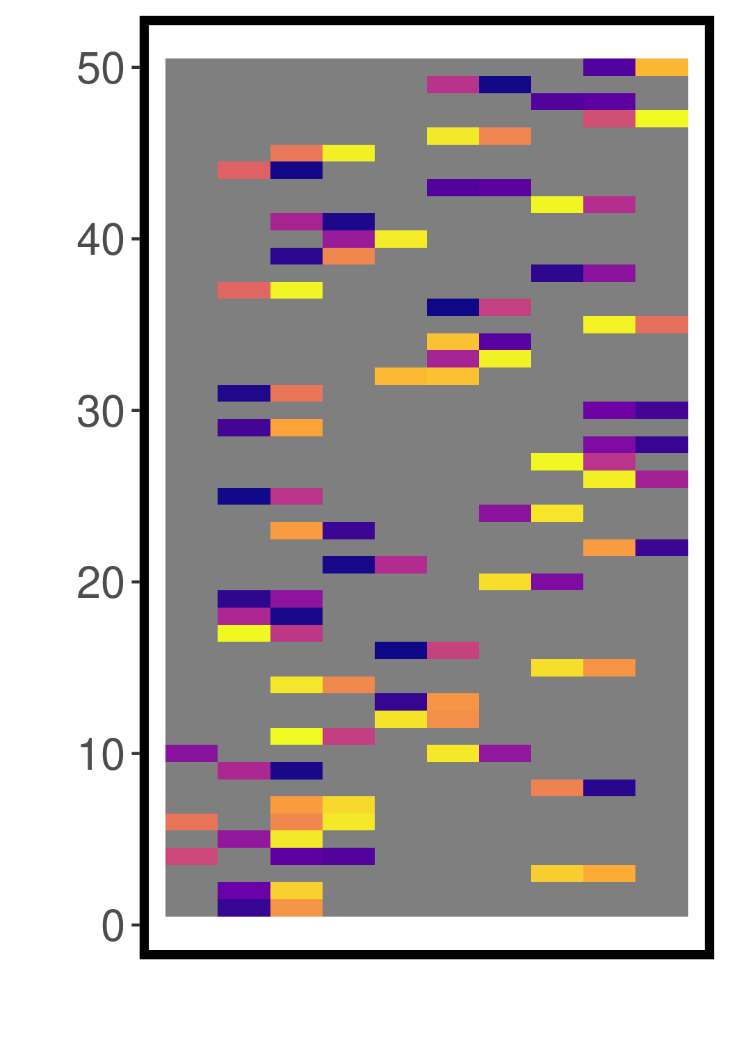

 |
The off-diagonals elements of are contributed entirely by . This allows to achieve sparsity in by inducing sparsity in . Following the discussion in Section 2.2.1, a carefully designed data-adaptive penalty on (e.g., a shrinkage prior on that sufficiently increases the probability of obtaining a sparse ) would induce sparsity in in such a (not necessarily unique) way that the sparsity patterns in are also accurately recovered. In this section, we show that by inducing sparsity in , sparsity is also induced in . We begin with the spike-and-slab prior (Ishwaran and Rao 2005) that allows exact zeros via a spike at zero and large nonzero elements via a continuous slab as
where is the prior probability of observing a zero for . For such priors can be analytically reduced to a simple form that helps gain insights into how inducing sparsity in can induce sparsity in with high probability. Specifically, since , where is the row of , can only happen when the entries of and are both not from the slab distribution for all . Therefore, we have
The behavior of for varying values of and are shown in Figure 4. It can be seen that by controlling , it is possible to induce any desired level of sparsity in . The hierarchical Beta prior on allows for data-adaptive learning and shrink the elements of accordingly (Scott and Berger 2010).

Implementation of spike-and-slab type mixture priors is computationally challenging. Thus, continuous global-local shrinkage priors have gained popularity in the Bayesian sparse estimation literature as they often greatly simplify posterior computation (Polson and Scott 2010) while retaining almost similar statistical properties of the classical spike-and-slab prior. In particular, we use the Dirichlet-Laplace (Bhattacharya et al. 2015, DL,) prior that has equivalent asymptotic properties with respect to the spike-and-slab in a similar context (Pati et al. 2014, Theorem 5.1) while being amenable to scalable posterior computation. The results for the spike-and-slab discussed here provides the intuitions on how continuous shrinkage priors like the DL induce sparsity in by inducing shrinkage on .
2.2.3 Advantages of the LRD Decomposition
For high-dimensional sparse covariance matrix estimation, this LRD decomposition strategy is extensively used in both Bayesian (Pati et al. 2014) and frequentist paradigms (Daniele et al. 2019) where the associated latent factor formulation allows scalable computation in big data problems (Bhattacharya and Dunson 2011; Fan et al. 2011; Sabnis et al. 2016; Fan et al. 2018; Kastner 2019, and others). Penalizing is thus a sensible approach to induce sparsity in . It also comes with many practical advantages described below.
Cholesky factorization based covariance and precision matrix estimation methods also use a similar strategy and penalize the lower triangular matrix to induce sparsity in (Dallakyan and Pourahmadi 2020). However, for undirected graphs, the estimates can vastly differ depending on the ordering of the variables (Kang and Deng 2020). In contrast, our proposed LRD decomposition based approach with a penalty on is invariant to the ordering of the variables.
In most existing approaches that directly penalize , frequentist or Bayesian, ensuring the positive definiteness of is also non-trivial, particularly in high dimensional settings. In frequentist regimes, for example, the graphical lasso (Friedman et al. 2008) does not guarantee positive definiteness of (Mazumder and Hastie 2012); similar behavior has also been observed for neighborhood selection methods (Meinshausen and Bühlmann 2006; Peng et al. 2009) and post-hoc treatments are required for positive definiteness. In Bayesian MAP approaches such as Gan et al. 2019, special care is needed in designing the optimization algorithm to ensure positive definiteness. For many existing Bayesian methods relying on MCMC (Wang 2012; Khondker et al. 2013; Li et al. 2019a), constrained update of in each step is difficult and expensive. Applications of these methods thus remain fairly limited to small to moderate dimensional problems. In contrast, the LRD formulation is always guaranteed to produce a positive definite estimate by construction.
As also discussed in the Introduction, posterior exploration is extremely challenging in Bayesian approaches that penalize the underlying the dense graphs first and then assign a prior on conditional on the graph, often requiring restrictive assumptions on the graph (Dawid and Lauritzen 1993) while still remaining computationally infeasible beyond only a few tens of dimensions (Jones et al. 2005). Our proposed approach on the other hand, works directly in the space, albeit via the LRD decomposition, avoiding having to define separate complex priors on the graph space thereby also avoiding restrictive assumptions on the graph while also achieving scalability far beyond such approaches via its latent factor representation.
2.3 Prior Specification
To accommodate high-dimensional data, with , it is crucial to reduce the effective number of parameters in the loadings matrix . A wide variety of sparsity inducing shrinkage priors for can be considered for this purpose. In this article, we employ a two-parameter generalization of the original Dirichlet-Laplace (DL) prior from Bhattacharya et al. 2015 that allows more flexible tail behavior. On a -dimensional vector , our DL prior with parameters and , denoted by , can be specified in the following hierarchical manner
where is the element of , is a vector of same length as , is an exponential distribution with mean , is the -dimensional Dirichlet distribution and is the gamma distribution with mean and variance . The original DL prior is a special case with . We let .
The column dimension of will almost always be unknown. Assigning a prior on and implementing a reversible jump MCMC (Green 1995) type algorithm can be inefficient and expensive. In this paper, we adopt an empirical Bayes type approach to set to a large value determined from the data and let the prior shrink the extra columns to zeros, substantially simplifying the computation. The strategy is discussed in greater details later in this section. We show in Section 2.6 that this approach is sufficient for the recovery of true under very mild conditions.
When , distinct ’s also result in over-parametrization. To reduce the number of parameters, we assume the ’s to comprise a small number of unique values. To achieve this in a data adaptive way, we use a Dirichlet process (DP) prior (Ferguson 1973) on the ’s as
| (6) |
where is the concentration parameter and is the base measure. Samples drawn from a DP are almost surely discrete, inducing a clustering of the ’s and thus reducing the dimension. Integrating out , model (6) leads to a recursive Polya urn scheme illustrative of the clustering mechanism while also being convenient for posterior computation (Escobar and West 1995; Neal 2000). Specifically, we have
where denote the unique values among and denote their multiplicities, being the latent variables such that if belongs to the cluster.
Choice of Hyperparameters: To specify the value of the latent dimension , we adopt a principal component analysis (PCA) based empirical Bayes type approach (Bai and Ng 2008). First, we perform a sparse PCA (Baglama and Reichel 2005) on the data matrix and compute the reciprocals of the singular values. We set to be the number of inverse singular values in decreasing order that adds up to of the total sum. We set and in all our simulation studies and real data applications. For the prior on the residual variances and the DP concentration parameter, we set .
2.4 Posterior Computation
The latent factor construction discussed in Section 2.1 leads to a novel, elegant Gibbs sampler that is operationally simple and free of any tuning parameter. There is also no need for additional constraints to ensure positive definiteness which used to be a major setback for MCMC based methods for precision matrix estimation. These features allow the sampler to be applied to dimensions far beyond the reach of the current state-of-the-art. Scalable posterior computation in LRD decomposed covariance matrix models is pretty standard in the literature but remained a major barrier for precision matrix models. The Gibbs sampler described here addresses this significant gap in the literature.
Starting with some initial values of and other parameters, our sampler iterates between the following steps. Other parameters and hyperparameters being implicitly understood in the conditioning, Step 1 defines a transition for ; Step 2 for (which is identical to ); Step 3 for (which is identical to ); and Steps 4 and 5 are standard updates for the parameters and hyper-parameters of the DL and DP priors, respectively.
- Step 1
-
Generate with independently from and let .
- Step 2
-
We have , where is the row of and . Define . Then . Conditioned on , and the associated hyper-parameters, ’s can be updated sequentially for from the distribution
where , and .
- Step 3
-
Sample the ’s through the following steps.
- (i)
Let and to be the collection of all ’s, , excluding . For , sample the cluster indicators sequentially from the distribution
The above integrals are analytically available and involves the density of a multivariate central Student’s -distribution for .
- (ii)
Let the unique values in be {. For , set and , and independently sample .
- (iii)
Set .
- (i)
- Step 4
-
Sample the hyper-parameters in the priors on through the following steps.
- (i)
For and sample independently from an inverse-Gaussian distribution and set .
- (ii)
Sample the full conditional posterior distribution of from a generalized inverse Gaussian distribution.
- (iii)
Draw independently with and set with .
- (i)
- Step 5
-
Following West 1992, first generate , evaluate and then generate
Remark 1.
Note that the main strategies underlying the algorithm above are not specific to the DL prior considered here. We are free to choose any other shrinkage prior that admits a conditionally Gaussian hierarchical representation for the entries of and modify Steps 2 and 4 accordingly. This is still a very large class of priors (Polson and Scott 2010), including, e.g., horseshoe (Carvalho et al. 2009), multiplicative gamma (Bhattacharya and Dunson 2011), etc. For non-conjugate priors, Steps 3 and 4 can also be modified with appropriate Metropolis-Hastings schemes. The other steps remain the same, making it a very broadly adaptable algorithm. An MCMC scheme for generic priors is outlined in Section S.1 of the supplementary materials.
Remark 2.
In the above sampler, the conditional posterior covariance matrix of is diagonal which allows us to update it with linear complexity. Thus, in each MCMC iteration, we only need a single small dimensional order matrix factorization operation in Step 1 to simulate . While high-dimensional matrix factorization operations are usally numerically very expensive, we are able to completely avoid that, facilitating substantial scalability.
Remark 3.
All but Steps 1 and 3 can be divided into parallel operations in a straightforward manner. Additionally, in recent versions of many popular statistical software, including R, matrix operations are inherently parallelized and hence Step 1 is also highly scalable in any decent computing system.
We implemented the Gibbs sampler in C++ and ported to R using the Rcpp package (Eddelbuettel and Francois 2011). In each case considered in this article, synthetic or real, we ran iterations which takes approximately 37 minutes on a system with an i9-10900K CPU and 64GB memory for a dimensional problem with sample size . The initial samples were discarded as burn-in and the remaining samples were thinned by an interval of . In all our experiments, convergence was swift and mixing was excellent. A comparison of the runtimes of our method and a few other existing methods is presented in Figure 5(c) below.
2.5 Graph Selection
As discussed in Section 2.2.2, the off-diagonals of are penalized by inducing shrinkage on . The theoretical results in Section 2.6 and numerical experiments in Section 3 show that, with our carefully constructed data adaptive shrinkage priors on , the inferred sparsity patterns in are such that a sparse is also accurately recovered (see Figures S.1 and 4(a) for estimates of sparse precision matrices obtained by our method). Exact zero estimates are, however, not obtained even for the insignificant off-diagonal elements of for finite samples. This is an artifact of continuous shrinkage priors, since the probabilities of exact zeroes are almost surely null for finite samples although the posterior probabilities of arbitrary sets around zeroes are very high.
We address the issue of non-zero edge selection through a novel multiple hypothesis testing based approach. For and some , we consider testing
| (7) |
where is the element of , the partial correlation matrix derived from . Here we follow Berger 1985 in replacing the point nulls by reasonable interval nulls . If is rejected in favor of , we conclude that there is an edge between nodes and .
We utilize posterior uncertainty to resolve these testing problems. Specifically, we define as the decision rule which controls the posterior FDR defined as
at the level . Importantly, the decision rule also incurs the lowest false non-discovery rate (Müller et al. 2004). For a fixed , the depends on the choice of . To obtain the optimal , we compute the ’s on a grid of values in and then set . This way, we have the FDR, that is, a quantified statistical uncertainty associated with the estimated graph. In all simulation experiments and real data applications in this paper, we control at the level of significance.
Remark 4.
Although this FDR control procedure is widely applicable, efficient posterior exploration is crucial for this step and hence may not be achievable or scalable to high dimensional problems when adapted to previously existing Bayesian approaches.
2.6 Posterior Concentration
Preliminaries and Notation: We let and denote the Frobenius and spectral norms of a matrix , respectively; be the smallest singular value of ; and be the eigenvalues of in decreasing order when is a -dimensional diagonalizable matrix. Also, and imply that and , respectively. Throughout, and are used to denote positive constants whose values might change from one line to the next but are independent from everything else. A -dimensional vector is said to be -sparse if only among the elements of are non-zero. We denote the set of all -sparse vectors in by .
We allow the model parameters to increase in dimensions with sample size , indicated by associating them with the suffix . We let denote the prior and the corresponding posterior given data , respectively.
Assumptions on the Data Generating Process: We assume that . In Section 2.2.1 we discussed how an LRD decomposition of a sparse can be constructed. Hence, we assume that admits the factor representation , where is a order sparse matrix and is a scalar. To simplify the theoretical analysis, we deviate here slightly from the proposed model and assume that the ’s all come from a single cluster with the common value . We show that the precision factor model with an appropriate DL prior can recover in ultra high-dimensional settings. As discussed in Section 2.3, we fix to a liberal large value and let the prior shrink the extra columns to zeros. We show that with appropriate sparsity conditions, the posterior of the precision factor model with the DL prior then concentrates around , even when the data dimension increases in exponential order with . The requisite conditions are stated below.
- (C1)
Let and be increasing sequences of positive integers such that , and .
- (C2)
is a order full rank matrix such that each column of belongs to , and .
- (C3)
The scalar lies in some compact set .
Specifics of the Postulated Precision Factor Model: Let be an increasing sequence of positive integers such that and . We assume that , where and is a matrix. We consider a prior on with and . We assume a gamma prior on independent of and truncated to the compact set .
Condition (C1) specifies the requisite sparsity conditions. It also imposes a condition on . Specifically, it can be seen that can be of exponential order of , allowing the recovery of massive precision matrices based on relatively small sample sizes. Note that, subject to appropriate orthogonal transformation, marginally . Conditions (C2) and (C3) ensure that these variances lie in a compact set. The prior specification provides a set of sufficient conditions on the class of proposed models. The true number of latent factors is also assumed smaller than the number of latent factors in the postulated models.
We let denote the class of precision matrices satisfying (C1)-(C3) and denote the class of positive definite matrices parametrized by in our precision factor model. Notably, can also be parametrized by . However, since , for a fixed , may be overparametrized for . In Theorem 1, we show that with increasing sample size, the posterior distribution supported on still concentrates around the true from . Using general results from Ghosal and van der Vaart 2017, we establish a convergence rate in terms of the operator norm. A rigorous proof is detailed in Section S.2 in the supplementary materials.
Theorem 1.
For any , and any sequence ,
In Section 2.2.1 we discussed a constructive way to find a sparse LRD decomposition of arbitrary sparse where the column dimension of need not exceed the number of non-zero off-diagonals of or edges in the conditional dependence graph. Theorem 1 implies that the precision matrix is recoverable if (C1) holds among others. Note that (C1) implies . Hence, can be learned from the data using the precision factor model as long as the number of edges is bounded by the sample size. Such assumptions are required to recover massive dimensional precision matrices from relatively smaller amount of data (Meinshausen and Bühlmann 2006; Ksheera Sagar et al. 2021).
Remark 5.
We derive a minimax lower bound of for the precision matrix estimation problem in Theorem 4 in the supplementary materials when which is a special case of (C1). The rate in Theorem 1 is times the lower bound. If we further let for some fixed positive integer , the rate attains the minimax lower bound up to a term.
Remark 6.
An interesting implication of our theoretical results is the robustness with respect to the choice of the latent dimension under very mild conditions. For the class of our postulated precision factor models, we err on the side of overestimating and let the DL prior shrink the extra factors to zero. The theoretical results imply that this strategy is sufficient to recover efficiently. The precise recovery rate, however, naturally depends on the choice of , a key parameter that distinguishes the class of postulated models from the class of true models (Shalizi 2009). The closer is to , the smaller the space to search for the truth, and the better the rate.
3 Simulation Studies
In this section, we discuss the results of some synthetic numerical experiments. We evaluate the performance of estimating the precision matrix itself as well as the underlying graph. We simulate data from three different cases - (i) a Gaussian autoregressive (AR) process of order 2, (ii) a multivariate Gaussian distribution with banded precision matrix, and (iii) a multivariate Gaussian distribution with randomly generated arbitrarily structured sparse (RSM) precision matrix. In all these cases, we take the mean vector to be zero. For plotting purposes in the RSM case, we assume two nodes to have an edge between them if the absolute value of the associated partial correlation exceeds and refer to this as the ‘true’ graph. We perform experiments for dimensions 50, 100, 200 and 1,000. For we take and for we take . We plot the true precision matrices and the associated true graphs for in Figure S.1 in the supplementary materials and in Figure 6(a) here in the main paper. For and we consider 50 and 20 independent replications for each scenario, respectively.
We apply our precision factor (PF) model to recover the precision matrices, using the posterior mean as our Bayesian point estimate. We compare it with the methods Bayesian graphical model under shrinkage (Gan et al. 2019, Bagus,), the graphical Lasso (Friedman et al. 2008, Glasso,) and the neighborhood selection by Meinshausen and Bühlmann 2006. We do not consider any previously existing Bayesian posterior sampling based methods here as they do not scale well beyond only a few tens of dimensions. We assess the comparative efficacy of these methods using qualitative graphical summaries as well as quantitative performance measures. For the proposed PF method, the graphs are estimated following the FDR control procedure outlined in Section 2.5. For Bagus, we follow the prescription in Section 4.3 of Gan et al. 2019. For in the banded case, the codes for Bagus did not work and we could not consider it as a competitor in that particular setup. For the other methods, the non-zero entries in the estimated precision matrix are considered as edges.
We compute the Frobenius norm between the true and estimated precision correlation matrices. To assess the accuracy of the derived graphs, we compute specificity and sensitivity , where (true positives), (false positives), (true negatives) and (false negatives) are based on the detection of the edges in the estimated graphs and comparing them with the corresponding true graphs. In Figure 5, the average values of these criteria across the replications are plotted for the competing methods. We also compare the execution times of the different methods.
From Figure 5, we see that, for banded precision matrices, the Frobenius norms obtained by our proposed PF method are very similar to those produced by the competitors. In the case of the arbitrarily structured precision matrix, however, the PF method performs much better, especially in higher dimensions. Also, the PF method yields much higher sensitivity in almost all the scenarios at the expense of slightly smaller specificity in some cases. This is expected since we are allowing a small margin of error by controlling the FDR at . Notably, the PF method is much more powerful in detecting the true edges. The other methods seem to be quite conservative in that regard, as seen in Figure 5(b). This explains the high Frobenius norm produced by the PF method in the AR(2) case with . The true precision matrix being extremely sparse with only two off-diagonals being non-zero, the conservative competitors are performing better in recovering the precision matrix in this particular setup. We see in Figure 5(c) that the PF method is slower than M&B and Glasso but is much faster than Bagus. Note however that, unlike the competitors, we are exploring the full posterior, not just providing a point estimate. On a related important note, since we are able to sample from the full posterior, unlike the other methods, we are able to provide a natural way of quantifying posterior uncertainty. Specifically, posterior credible intervals for each element of the precision matrix can be obtained from the MCMC samples. For and sample size , we plot the lower and upper quantiles of the entry-wise partial correlations along with the simulation truths in Figure S.1 in the supplementary materials. The plots indicate that the simulation truths are well-within the confidence bounds.
Circos plots (Gu et al. 2014) of the true and estimated graphs are shown in Figure 7. For the AR(2) case, none of the methods are doing well in recovering the graph. For the other cases, the proposed PF method outperforms the competitors. Figures S.3 and S.5 in the supplementary materials provide alternate graphical representations useful in visually discerning the superior performance of the PF method.


4 Application
We applied our proposed method to two real data sets from two different application domains, namely genomics and finance. To meet space constraints, the finance application is presented separately in Section S.4 in the supplementary materials.
Immune cells serve specialized roles in innate and adaptive bodily responses to eliminate antigens. To understand the cell biology of carcinogenic processes, study of immune cells and the genes therein are thus of immense importance.
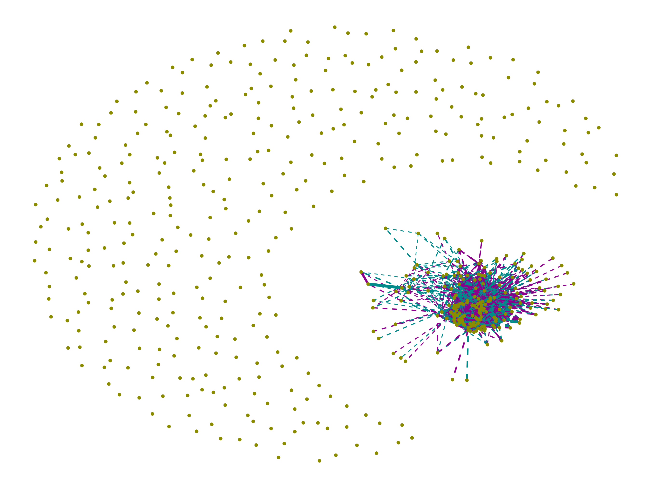


We obtain the data from the Immunological Genome Project (ImmGen) data browser (Heng et al. 2008). ImmGen is a collaborative scientific research project that is currently building a gene-expression database for all characterized immune cells in mice. In particular, we use the GSE15907 microarray dataset (Painter et al. 2011; Desch et al. 2011) comprising of multiple immune cell lineages which were isolated ex-vivo, primarily from young adult B6 male mice and double-sorted to purity. The cell population includes all adaptive and innate lymphocytes (B, abT, gdT, Innate-Like Lymphocytes), myeloid cells (dendritic cells, macrophages, monocytes), mast cells and neutrophils. The already normalized dataset has more than gene expressions from immune cells. We made a transformation of the data and filtered the top genes with highest variances using the genefilter R package (Gentleman et al. 2020), resulting in a dimensional problem. Since different cell-types exhibit very different gene expression profiles, we centered the gene-expressions separately within each cell type. The estimated graph corresponding to all genes is shown in Figure 8(a). We can see clear evidence towards conditional independence between most of the genes, indicating that only a small subset of genes are functionally responsible for the variability.
For more insights, we zoom into the connected genes and plot the corresponding partial correlation matrix and graph, limited to the genes possessing at least 5 edges, in Figures 8(b) and 8(c) respectively. We notice overall positive partial correlations between the histone class of genes such as Hist2h3b, Hist1h3h, Hist2h3c1, Hist1h3c, etc (Wolffe 2001). The positive correlations between these protein coding genes indicate that these genes are generally expressed together in the mechanism. Bcl2a1a and Bcl2a1d, two functional isoforms of the B cell leukemia 2 family member A1 exerting important pro-survival functions, show strong positive association. We also observe strong positive association between Ly6c1 and Ly6c2 genes. Lee et al. 2013 noted these genes to be located adjacent to each other in the mid‐section of the Ly6 complex. They share similarity in their genomic and protein sequences and these two genes has been considered synonymous to each other and hence exhibit strong positive association. Although positive correlations are often observed between the membrane-spanning 4A class of genes such as Ms4a4c, Ms4a4b, Ms4a6b, etc. (Liang et al. 2001), we find the genes to be conditionally almost independent in our analysis. It indicates that their expressions might be regulated by other genes.
From Figure 8(b), it thus seems that there exist two blocks where within each block the genes are positively associated whereas between the blocks the genes are negatively associated. This might again be an indication that either of these blocks of genes are generally expressed together in immune cells.
5 Discussion
In this article, we proposed a novel flexible statistical model for Gaussian precision matrices that relies on decomposing them into a low-rank and a diagonal component. The decomposition is theoretically and practically highly flexible and is thus often used in covariance matrix models, arising naturally in their computationally tractable latent factor based representations. The approach has, however, not been popular in precision matrix and related graph estimation problems as it poses daunting computational challenges when applied to such settings. We addressed this issue in this article by exploring a previously under-utilized latent variable construction, leading to a highly scalable Gibbs sampler that allows efficient posterior inference. The decomposition based strategy also allowed us to use sparsity inducing priors to shrink insignificant off-diagonal entries toward zero while also making the approach adaptable to high-dimensional sparse settings. We specifically adapted the Dirichlet-Laplace prior for sparse precision matrix estimation. We developed a novel posterior FDR control based method to perform graph selection that properly accommodates posterior uncertainty. We also established theoretical convergence guarantees for the proposed model in high-dimensional sparse settings. In synthetic experiments, the proposed method vastly outperformed its competitors in receiving the true underlying graphs. We illustrated the method’s practical utility through real data examples from genomics and finance.
Aside from providing fundamentally new probabilistic perspectives on Gaussian precision matrix and related graph estimation problems, our work also bridges the gap between frequentist penalized likelihood based strategies and Bayesian shrinkage prior based ideas for such models. The simple and highly scalable computational algorithms resulting from our latent factor representation should also free up Bayesians from having to put restrictive assumptions on the graph structures to achieve computational tractability, opening up new opportunities to adapt the basic models to more complex and more realistic data structures and study designs. A few such methodological extensions we are pursuing as topics of separate ongoing research include dynamic Gaussian graphical models (Huang and Chen 2017), covariate dependent Gaussian graphical models, nonparanormal (Liu et al. 2009) and Gaussian copula graphical models (Pitt et al. 2006), etc.
Supplementary Materials
Supplementary materials discuss a general strategy for posterior computation under broad classes of generic priors, proofs of the theoretical results, some additional figures, and an application to a NASDAQ-100 stock price dataset.
References
- Armstrong et al. (2009) Armstrong, H., Carter, C. K., Wong, K. F. K., and Kohn, R. (2009). Bayesian covariance matrix estimation using a mixture of decomposable graphical models. Statistics and Computing, 19, 303–316.
- Atay-Kayis and Massam (2005) Atay-Kayis, A. and Massam, H. (2005). A Monte Carlo method for computing the marginal likelihood in nondecomposable Gaussian graphical models. Biometrika, 92, 317–335.
- Baglama and Reichel (2005) Baglama, J. and Reichel, L. (2005). Augmented implicitly restarted Lanczos bidiagonalization methods. SIAM Journal on Scientific Computing, 27, 19–42.
- Bai and Ng (2008) Bai, J. and Ng, S. (2008). Large dimensional factor analysis. Foundations and Trends in Econometrics, 3, 89–163.
- Banerjee et al. (2008) Banerjee, O., El Ghaoui, L., and d’Aspremont, A. (2008). Model selection through sparse maximum likelihood estimation for multivariate Gaussian or binary data. JMLR, 9, 485–516.
- Banerjee and Ghosal (2015) Banerjee, S. and Ghosal, S. (2015). Bayesian structure learning in graphical models. Journal of Multivariate Analysis, 136, 147–162.
- Barvinok and Rudelson (2022) Barvinok, A. and Rudelson, M. (2022). When a system of real quadratic equations has a solution. Advances in Mathematics, 403, 108391.
- Berger (1985) Berger, J. O. (1985). Statistical decision theory and Bayesian analysis. Springer series in statistics. Springer-Verlag, New York, 2nd edition.
- Bhattacharya and Dunson (2011) Bhattacharya, A. and Dunson, D. B. (2011). Sparse Bayesian infinite factor models. Biometrika, 98, 291–306.
- Bhattacharya et al. (2015) Bhattacharya, A., Pati, D., Pillai, N. S., and Dunson, D. B. (2015). Dirichlet-Laplace priors for optimal shrinkage. Journal of the American Statistical Association, 110, 1479–1490.
- Bhattacharya et al. (2016) Bhattacharya, A., Chakraborty, A., and Mallick, B. K. (2016). Fast sampling with Gaussian scale mixture priors in high-dimensional regression. Biometrika, 103, 985–991.
- Bien and Tibshirani (2011) Bien, J. and Tibshirani, R. J. (2011). Sparse estimation of a covariance matrix. Biometrika, 98, 807–820.
- Carvalho and Scott (2009) Carvalho, C. M. and Scott, J. G. (2009). Objective Bayesian model selection in Gaussian graphical models. Biometrika, 96, 497–512.
- Carvalho et al. (2007) Carvalho, C. M., Massam, H., and West, M. (2007). Simulation of hyper-inverse Wishart distributions in graphical models. Biometrika, 94, 647–659.
- Carvalho et al. (2009) Carvalho, C. M., Polson, N. G., and Scott, J. G. (2009). Handling sparsity via the horseshoe. In Artificial Intelligence and Statistics, pages 73–80. PMLR.
- Chandra and Bhattacharya (2019) Chandra, N. K. and Bhattacharya, S. (2019). Non-marginal decisions: A novel Bayesian multiple testing procedure. Electronic Journal of Statistics, 13, 489–535.
- Dallakyan and Pourahmadi (2020) Dallakyan, A. and Pourahmadi, M. (2020). Fused-lasso regularized Cholesky factors of large nonstationary covariance matrices of longitudinal data. arXiv:2007.11168.
- Daniele et al. (2019) Daniele, M., Pohlmeier, W., and Zagidullina, A. (2019). Sparse approximate factor estimation for high-dimensional covariance matrices. arXiv:1906.05545.
- d’Aspremont et al. (2008) d’Aspremont, A., Banerjee, O., and El Ghaoui, L. (2008). First-order methods for sparse covariance selection. SIAM Journal on Matrix Analysis and Applications, 30, 56–66.
- Dawid and Lauritzen (1993) Dawid, A. P. and Lauritzen, S. L. (1993). Hyper Markov laws in the statistical analysis of decomposable graphical models. The Annals of Statistics, 21, 1272–1317.
- Dellaportas et al. (2003) Dellaportas, P., Giudici, P., and Roberts, G. (2003). Bayesian inference for nondecomposable graphical Gaussian models. Sankhyā: The Indian Journal of Statistics, pages 43–55.
- Desch et al. (2011) Desch, A. N., Randolph, G. J., et al. (2011). CD103+ pulmonary dendritic cells preferentially acquire and present apoptotic cell–associated antigen. Journal of Experimental Medicine, 208, 1789–1797.
- Deshpande et al. (2019) Deshpande, S. K., Ročková, V., and George, E. I. (2019). Simultaneous variable and covariance selection with the multivariate spike-and-slab lasso. Journal of Computational and Graphical Statistics, 28, 921–931.
- Dobra et al. (2004) Dobra, A., Hans, C., Jones, B., Nevins, J. R., Yao, G., and West, M. (2004). Sparse graphical models for exploring gene expression data. Journal of Multivariate Analysis, 90, 196–212.
- Dobra et al. (2011) Dobra, A., Lenkoski, A., and Rodriguez, A. (2011). Bayesian inference for general Gaussian graphical models with application to multivariate lattice data. Journal of the American Statistical Association, 106, 1418–1433.
- Eddelbuettel and Francois (2011) Eddelbuettel, D. and Francois, R. (2011). Rcpp: Seamless R and C++ integration. Journal of Statistical Software, 40, 1–18.
- Escobar and West (1995) Escobar, M. D. and West, M. (1995). Bayesian density estimation and inference using mixtures. Journal of the American Statistical Association, 90, 577–588.
- Fan et al. (2011) Fan, J., Liao, Y., and Mincheva, M. (2011). High-dimensional covariance matrix estimation in approximate factor models. The Annals of Statistics, 39, 3320–3356.
- Fan et al. (2018) Fan, J., Liu, H., and Wang, W. (2018). Large covariance estimation through elliptical factor models. The Annals of Statistics, 46, 1383–1414.
- Ferguson (1973) Ferguson, T. S. (1973). A Bayesian analysis of some nonparametric problems. The Annals of Statistics, 1, 209–230.
- Friedman et al. (2008) Friedman, J., Hastie, T., and Tibshirani, R. (2008). Sparse inverse covariance estimation with the graphical lasso. Biostatistics, 9, 432–441.
- Gan et al. (2019) Gan, L., Narisetty, N. N., and Liang, F. (2019). Bayesian regularization for graphical models with unequal shrinkage. Journal of the American Statistical Association, 114, 1218–1231.
- Gentleman et al. (2020) Gentleman, R., Carey, V., Huber, W., and Hahne, F. (2020). genefilter: methods for filtering genes from high-throughput experiments. R package version 1.70.0.
- Ghosal and van der Vaart (2017) Ghosal, S. and van der Vaart, A. (2017). Fundamentals of nonparametric Bayesian inference. Cambridge Series in Statistical and Probabilistic Mathematics. Cambridge University Press.
- Green (1995) Green, P. J. (1995). Reversible jump Markov chain Monte Carlo computation and Bayesian model determination. Biometrika, 82, 711–732.
- Green and Thomas (2013) Green, P. J. and Thomas, A. (2013). Sampling decomposable graphs using a Markov chain on junction trees. Biometrika, 100, 91–110.
- Gu et al. (2014) Gu, Z., Gu, L., Eils, R., Schlesner, M., and Brors, B. (2014). circlize implements and enhances circular visualization in R. Bioinformatics, 30, 2811–2812.
- Heng et al. (2008) Heng, T. S., Painter, M. W., Elpek, K., Lukacs-Kornek, V., Mauermann, N., Turley, S. J., Koller, D., Kim, F. S., Wagers, A. J., Asinovski, N., et al. (2008). The immunological genome project: networks of gene expression in immune cells. Nature Immunology, 9, 1091–1094.
- Huang and Chen (2017) Huang, F. and Chen, S. (2017). Learning dynamic conditional Gaussian graphical models. IEEE Transactions on Knowledge and Data Engineering, 30, 703–716.
- Ishwaran and Rao (2005) Ishwaran, H. and Rao, J. S. (2005). Spike and slab variable selection: Frequentist and Bayesian strategies. The Annals of Statistics, 33, 730–773.
- Jones et al. (2005) Jones, B., Carvalho, C., Dobra, A., Hans, C., Carter, C., and West, M. (2005). Experiments in stochastic computation for high-dimensional graphical models. Statistical Science, 20, 388–400.
- Kang and Deng (2020) Kang, X. and Deng, X. (2020). An improved modified Cholesky decomposition approach for precision matrix estimation. Journal of Statistical Computation and Simulation, 90, 443–464.
- Kastner (2019) Kastner, G. (2019). Sparse Bayesian time-varying covariance estimation in many dimensions. Journal of Econometrics, 210, 98–115.
- Khare et al. (2018) Khare, K., Rajaratnam, B., and Saha, A. (2018). Bayesian inference for Gaussian graphical models beyond decomposable graphs. Journal of the Royal Statistical Society: Series B: Statistical Methodology, 80, 727–747.
- Khondker et al. (2013) Khondker, Z. S., Zhu, H., Chu, H., Lin, W., and Ibrahim, J. G. (2013). The Bayesian covariance lasso. Statistics and its Interface, 6, 243.
- Koller and Friedman (2009) Koller, D. and Friedman, N. (2009). Probabilistic graphical models: Principles and techniques. MIT press.
- Ksheera Sagar et al. (2021) Ksheera Sagar, K. N., Banerjee, S., Datta, J., and Bhadra, A. (2021). Precision matrix estimation under the horseshoe-like prior-penalty dual. arXiv:2104.10750.
- Lauritzen (1996) Lauritzen, S. L. (1996). Graphical models. Clarendon Press.
- Lee et al. (2013) Lee, P. Y., Wang, J.-X., et al. (2013). Ly6 family proteins in neutrophil biology. Journal of Leukocyte Biology, 94, 585–594.
- Lenkoski (2013) Lenkoski, A. (2013). A direct sampler for G-Wishart variates. Stat, 2, 119–128.
- Levina et al. (2008) Levina, E., Rothman, A., and Zhu, J. (2008). Sparse estimation of large covariance matrices via a nested Lasso penalty. The Annals of Applied Statistics, 2, 245–263.
- Li et al. (2019a) Li, Y., Craig, B. A., and Bhadra, A. (2019a). The graphical horseshoe estimator for inverse covariance matrices. Journal of Computational and Graphical Statistics, 28, 747–757.
- Li et al. (2019b) Li, Z., Mccormick, T., and Clark, S. (2019b). Bayesian joint spike-and-slab graphical lasso. In International Conference on Machine Learning, pages 3877–3885. PMLR.
- Liang et al. (2001) Liang, Y., Buckley, T. R., et al. (2001). Structural organization of the human MS4A gene cluster on chromosome 11q12. Immunogenetics, 53, 357–368.
- Liu et al. (2009) Liu, H., Lafferty, J., and Wasserman, L. (2009). The nonparanormal: Semiparametric estimation of high dimensional undirected graphs. Journal of Machine Learning Research, 10, 2295–2328.
- Mazumder and Hastie (2012) Mazumder, R. and Hastie, T. (2012). The graphical lasso: New insights and alternatives. Electronic Journal of Statistics, 6, 2125–2149.
- Meinshausen and Bühlmann (2006) Meinshausen, N. and Bühlmann, P. (2006). High-dimensional graphs and variable selection with the Lasso. The Annals of Statistics, 34, 1436–1462.
- Mitra et al. (2013) Mitra, R., Müller, P., Liang, S., Yue, L., and Ji, Y. (2013). A Bayesian graphical model for chip-seq data on histone modifications. Journal of the American Statistical Association, 108, 69–80.
- Mohammadi and Wit (2015) Mohammadi, A. and Wit, E. C. (2015). Bayesian structure learning in sparse Gaussian graphical models. Bayesian Analysis, 10, 109–138.
- Mohammadi et al. (2021) Mohammadi, R., Massam, H., and Letac, G. (2021). Accelerating Bayesian structure learning in sparse Gaussian graphical models. Journal of the American Statistical Association. To appear.
- Müller et al. (2004) Müller, P., Parmigiani, G., Robert, C., and Rousseau, J. (2004). Optimal sample size for multiple testing: The case of gene expression microarrays. Journal of the American Statistical Association, 99, 990–1001.
- Neal (2000) Neal, R. M. (2000). Markov chain sampling methods for Dirichlet process mixture models. Journal of Computational and Graphical Statistics, 9, 249–265.
- Painter et al. (2011) Painter, M. W., Davis, S., Hardy, R. R., Mathis, D., Benoist, C., Consortium, I. G. P., et al. (2011). Transcriptomes of the B and T lineages compared by multiplatform microarray profiling. The Journal of Immunology, 186, 3047–3057.
- Pati et al. (2014) Pati, D., Bhattacharya, A., Pillai, N. S., and Dunson, D. (2014). Posterior contraction in sparse Bayesian factor models for massive covariance matrices. The Annals of Statistics, 42, 1102–1130.
- Peng et al. (2009) Peng, J., Wang, P., Zhou, N., and Zhu, J. (2009). Partial correlation estimation by joint sparse regression models. Journal of the American Statistical Association, 104, 735–746.
- Pitt et al. (2006) Pitt, M., Chan, D., and Kohn, R. (2006). Efficient Bayesian inference for Gaussian copula regression models. Biometrika, 93, 537–554.
- Polson and Scott (2010) Polson, N. G. and Scott, J. G. (2010). Shrink globally, act locally: Sparse Bayesian regularization and prediction. Bayesian Statistics, 9, 1–24.
- Pourahmadi (2013) Pourahmadi, M. (2013). High-dimensional covariance estimation. John Wiley & Sons.
- Rothman et al. (2008) Rothman, A. J., Bickel, P. J., Levina, E., Zhu, J., et al. (2008). Sparse permutation invariant covariance estimation. Electronic Journal of Statistics, 2, 494–515.
- Roverato (2002) Roverato, A. (2002). Hyper inverse Wishart distribution for non-decomposable graphs and its application to Bayesian inference for Gaussian graphical models. Scandinavian Journal of Statistics, 29, 391–411.
- Sabnis et al. (2016) Sabnis, G., Pati, D., Engelhardt, B., and Pillai, N. (2016). A divide and conquer strategy for high dimensional Bayesian factor models. arXiv preprint arXiv:1612.02875.
- Scott and Berger (2010) Scott, J. G. and Berger, J. O. (2010). Bayes and empirical-Bayes multiplicity adjustment in the variable-selection problem. The Annals of Statistics, 38, 2587–2619.
- Shalizi (2009) Shalizi, C. R. (2009). Dynamics of Bayesian updating with dependent data and misspecified models. Electronic Journal of Statistics, 3, 1039–1074.
- Wang (2012) Wang, H. (2012). Bayesian graphical lasso models and efficient posterior computation. Bayesian Analysis, 7, 867–886.
- West (1992) West, M. (1992). Hyperparameter estimation in Dirichlet process mixture models. Duke University ISDS Discussion Paper# 92-A03.
- Witten et al. (2011) Witten, D. M., Friedman, J. H., and Simon, N. (2011). New insights and faster computations for the graphical lasso. Journal of Computational and Graphical Statistics, 20, 892–900.
- Wolffe (2001) Wolffe, A. (2001). Histone genes. In Encyclopedia of Genetics, pages 948–952. Academic Press, New York.
- Yoshida and West (2010) Yoshida, R. and West, M. (2010). Bayesian learning in sparse graphical factor models via variational mean-field annealing. Journal of Machine Learning Research, 11, 1771–1798.
- Yuan and Lin (2007) Yuan, M. and Lin, Y. (2007). Model selection and estimation in the Gaussian graphical model. Biometrika, 94, 19–35.
- Zhang and Zou (2014) Zhang, T. and Zou, H. (2014). Sparse precision matrix estimation via lasso penalized D-trace loss. Biometrika, 101, 103–120.
- Zhu et al. (2014) Zhu, H., Khondker, Z., Lu, Z., and Ibrahim, J. G. (2014). Bayesian generalized low rank regression models for neuroimaging phenotypes and genetic markers. Journal of the American Statistical Association, 109, 977–990.
Supplementary Materials for
Bayesian Scalable Precision Factor
Analysis
for Massive Sparse
Gaussian Graphical Models
Noirrit Kiran Chandraa (noirrit.chandra@utdallas.edu)
Peter Müllerb,c (pmueller@math.utexas.edu)
Abhra Sarkarb (abhra.sarkar@utexas.edu)
aDepartment of Mathematical Sciences,
The University of Texas at Dallas,
800 W. Campbell Rd, Richardson, TX 75080-3021, USA
bDepartment of Statistics and Data Sciences,
The University of Texas at Austin,
2317 Speedway D9800, Austin, TX 78712-1823, USA
cDepartment of Mathematics,
The University of Texas at Austin,
2515 Speedway, PMA 8.100, Austin, TX 78712-1823, USA
Supplementary materials discuss a general strategy for posterior computation under a broad class of generic priors, proofs of the theoretical results, some additional figures, and an application to a NASDAQ-100 stock price dataset.
S.1 General Strategy for Posterior Computation
In this section, we sketch out a general strategy for posterior inference for the precision factor model not limited to the prior specifications in Section 2.3.
- Sampling model:
-
The data generating mechanism, we recall, is
where is a dimensional matrix with and .
- Generic priors:
-
We consider the following broad classes of hierarchical priors on and with and being the respective associated hyperparameters
Varying choices of then produce a broad class of priors for the model parameters.
The Gibbs sampler then iterates through the following steps.
- Step 1. Sample the latent variables:
-
Generate with independently from and let .
- Step 2. Sample the rows of :
-
We have , where is the row of and . Define . Then . Conditioned on , and the associated hyper-parameters, ’s can be updated sequentially from the following posterior distribution
where is the prior covariance matrix of , and .
- Step 3. Sample :
-
Sample from .
- Step 4. Sample the hyperparameters of :
-
Sample from .
- Step 5. Sample the hyperparameters of :
-
Sample from .
For non-conjugate priors, appropriate Metropolis-within-Gibbs type MCMC algorithms can be employed in Steps 2, 3, 4 or 5.
S.2 Proofs of Theoretical Results
Notations: In what follows, for an operation ‘’, is sometimes used for . Also, for two sequences , implies that for some constant ; implies that . denotes the determinant of the square matrix . For a set , denotes its cardinality. Let is the Euclidean norm of a vector . We denote the Kullback-Leibler (KL) divergence between two mean zero Gaussian distributions with precision matrices and by . We borrow the following result from Pati et al. 2014 (Lemma 1.1. from the supplement). For brevity of notations, we reuse , , , etc. in the proofs to denote constants and their values may not be the same throughout the same proof. Nevertheless, we were careful to make sure that these quantities are indeed constants.
Lemma 1.
For any two matrices and ,
- (i)
.
- (ii)
.
- (iii)
.
Theorem 1.
Let be an arbitrary partition. Note that,
To prove the theorem, we show that, as , the posterior distribution on concentrates around while the remaining mass assigned to diminishes to zero. We adopt a variation of Theorem 8.22 by Ghosal and van der Vaart 2017 on posterior contraction rates. Define . We now formally state the result tailored towards our application.
Theorem 2.
Let be a class of distributions prametrized by , the corresponding distribution and be the true data-generating value of the parameter. Let be a metric on and . For constants with and every sufficiently large , assume the following conditions hold.
- (i)
For some , ;
- (ii)
Define the set . There exists tests such that, for some ,
Then, in -probability for any .
We define , , and for some large enough constant . We verify (i) in Lemma 3 and show the existence of a sequence of test functions satisfying (ii) in Lemma 4. Hence,
Subsequently applying the dominated convergence theorem (DCT), we get . To conclude the proof, we show that the remaining mass assigned to goes to 0 in the following theorem.
Theorem 3.
.
∎
Theorem 2.
The theorem closely resembles Theorem 8.22 from Ghosal and van der Vaart 2017. In the discussion following equation (8.22) in the book, the authors noted that for the iid case, simpler theorems are obtained by using an absolute lower bound on the prior mass and by replacing the local entropy by the global entropy. In particular, (i) implies Theorem 8.19(i) in the book. Similarly, (ii) is the same condition in Theorem 8.20 and hence the proof. ∎
Lemma 2.
(Kullback-Leibler upper bound) Let and be order positive definite matrices. Then,
Proof.
Lemma 3.
Define the set . Then, for and some absolute constant .
Proof.
From Lemma 2, we note that
| (S.4) |
We handle the and parts in (S.4) separately and conclude the proof by showing that each of the terms individually exceeds for some constant .
The part in (S.4): We define , after augmenting null columns to . Also . Invoking (C2) and Lemma 1, we have that implies that for some . Note that, from (C2) and (C3), . Let denote the vector of elements of corresponding to an index set , and denote the set of nonzero elements in . Then, for some absolute constant , we have
| (S.5) |
The first term in (S.5) ensures that the Bayesian model assigns requisite prior mass around the signals whereas the second term ensures that appropriate shrinkage is envisaged through the prior. We show that each of these products exceeds .
- The shrinkage part in (S.5):
-
From Bhattacharya et al. 2015, we get that where ’s are marginally iid random variables with a priori with pdf where is the modified Bessel function of the second kind. Using Lemma 3.2 of the same paper and letting , we have
Now, and . Since and is an increasing sequence, and hence
The second last inequality in the previous equation follows since, for any and , we have .
- The signal part in (S.5):
-
Let us define to be the -dimensional Euclidean ball of radius centered at zero and denotes its volume. For the sake of brevity, denote , so that . Letting (’s defined earlier) and , we have
(S.6) Note that, and and using Castillo and van der Vaart 2012, . Note also that for , which implies that . Hence,
The last inequality follows from (C1) and the prior specifications. From Bhattacharya et al. 2015 we have
Corollary 1.
For arbitrary , we have for some constant .
Following the proof of Lemma 3, it can be seen that the above corollary holds.
Lemma 4.
Let and the set denote an annulus of inner radius and outer radius , where , in operator norm around for some integer . Based on iid samples from , consider the following hypothesis testing problem
We simulate , with independently from and define . Letting , we define the following test function . Then
for some absolute constant .
Proof.
- Type-I error:
-
Under , we have . Letting , we have, , where from (C2). From Vershynin 2012, for a universal constant and any sequence satisfying . Since from (C1), and as , can be constructed such that and hence .
- Type-II error:
-
If with , then where . Notably, . Now,
(S.7) where . By construction of , for . Hence, for , the RHS of (S.7) is bounded below by for sufficiently large . Using Vershynin 2012 again, we have for all , .
Hence the proof. ∎
Theorem 3.
For densities and , define . When and are mean zero multivariate Gaussian densities with precision matrices and , we simply denote . We define the set .
From Banerjee and Ghosal 2015 and the proof of Lemma 2, we have and therefore for some constant .
Let be an increasing sequence of positive numbers. Then, for some constant where is the norm. The last inequality follows from Pati et al. 2014. Hence, for ,
From Corollary 1, for arbitrary , . Hence, for . The last display holds for suitable large enough choice of , which, however, can be chosen independent of . Using Ghosal and van der Vaart 2017 and subsequent application of DCT we conclude the proof. ∎
Theorem 4 (minimax rate).
If is a sequence of estimators of with , then for some absolute constant
Proof.
We use Fano’s lemma to derive a lower bound for the minimax risk. Let , be a finite subset of and let be an estimate of based on iid samples . Suppose for all , we have for some metric and . Letting denote the expectation under , Fano’s lemma (Yu 1997) implies
| (S.8) |
We now construct the finite class . Let . Define to be the collection of all binary vectors of length with exactly ones and let be the Hamming distance between two binary vectors and . Let denote the -dimensional vector obtained by appending zero at the end of with . With this definitions, set where is the vector with 1 in the coordinate and zero elsewhere, and are positive sequences to be chosen below.
Observe that if for , then . Note also that . The nonzero eigenvalues of the matrix are , since , and . This implies that . Since for all , by symmetry for all . Hence . Let , where is a diagonal matrix with the first diagonals equaling one and the entry being . Subsequently, applying the Woodbury matrix inversion identity, we get so that with . Observing that and , we get .
Now, from Pati et al. 2014, given , there exists a subset of with and for all , where is a positive constant independent of . We set . Using the aforementioned lemma and preceding discussions, we have that is bounded above by fo all pairs . Hence, we can choose and in (S.8). To obtain as a lower bound to the minimax risk up to a constant, we set for some . Since , we obtain by choosing , that . ∎
S.3 Additional Figures
S.3.1 Uncertainty Quantification


S.3.2 Graph Estimation
True and estimated graphs derived from the respective precision matrices as described in Section 3 of the main paper using the GGally package (Schloerke et al. 2020) in R.


S.3.3 Precision Matrix Estimation


S.4 NASDAQ-100 Stock Price Data
Here we apply the precision factor model to a stock price dataset comprising the top 100 companies listed in NASDAQ for the period Jan 2015 - Dec 2019 recorded every week. We obtained the data from Yahoo finance. After removing missing records, we ended up with data on 91 companies. First, we removed the trend by linear trend fitting. The estimated graph shown in Figure S.6 indicates a sparse structure.
We highlight some interesting features observed from the analysis. We observe a strong positive association between the rival GPU developers AMD and Nvidia Corporation (NVDA) consistent with the increasing demand of GPU computing. Similarly, a positive association between Qualcomm (QCOM) and Marvell Technology Group (MRVL), both of which develop and produce semiconductors and related technology, can be seen. The electronic design automation company Synopsys (SNPS) and the software company Cadence Design Systems, Inc. (CDNS) exhibit strong positive associations. Electronic Arts (EA) and Activision (ATVI) are video game developers and a Positive association is observed between them. ATVI seem to have strong associations with Amazon.com, Inc. (AMZN) and Apple Inc (AAPL). The semiconductor manufacturer companies Texas Instruments (TXN) and Xilinx (XLNX) seem to have a negative association. We observe positive association between the computer memory and data storage producing company Micron Technology, Inc. (MU) and Match Group (MTCH). Interestingly, the American semiconductor company Skyworks Solutions, Inc. (SWKS) exhibit strong negative association with companies like Microsoft (MSFT), Comcast Corporation (CMCSA), MU, etc. Many of the aforementioned stocks exhibit strong positive association with the Meta Platforms, Inc. (FB) previously known as Facebook Inc. As expected, we observe a strong positive association between GOOGL and GOOG, which are Google shares with and without voting rights, respectively.
Notably, most of the connected nodes in the NASDAQ-100 listing correspond to technology companies and electronics manufacturers. This is in accordance with the ushering in of the ‘digital era’ over the last decade, with technology giants taking over major shares of the market. Also, the strong negative associations between several companies in similar domains reflect the competitive nature of the market.
References
- Banerjee and Ghosal (2015) Banerjee, S. and Ghosal, S. (2015). Bayesian structure learning in graphical models. Journal of Multivariate Analysis, 136, 147–162.
- Bhattacharya et al. (2015) Bhattacharya, A., Pati, D., Pillai, N. S., and Dunson, D. B. (2015). Dirichlet-Laplace priors for optimal shrinkage. Journal of the American Statistical Association, 110, 1479–1490.
- Castillo and van der Vaart (2012) Castillo, I. and van der Vaart, A. (2012). Needles and straw in a haystack: Posterior concentration for possibly sparse sequences. The Annals of Statistics, 40, 2069–2101.
- Ghosal and van der Vaart (2017) Ghosal, S. and van der Vaart, A. (2017). Fundamentals of nonparametric Bayesian inference. Cambridge Series in Statistical and Probabilistic Mathematics. Cambridge University Press.
- Pati et al. (2014) Pati, D., Bhattacharya, A., Pillai, N. S., and Dunson, D. (2014). Posterior contraction in sparse Bayesian factor models for massive covariance matrices. The Annals of Statistics, 42, 1102–1130.
- Schloerke et al. (2020) Schloerke, B., Cook, D., Larmarange, J., Briatte, F., Marbach, M., Thoen, E., Elberg, A., and Crowley, J. (2020). GGally: Extension to ‘ggplot2’. R package version 2.0.0.
- Vershynin (2012) Vershynin, R. (2012). Introduction to the non-asymptotic analysis of random matrices, page 210–268. Cambridge University Press.
- Yu (1997) Yu, B. (1997). Assouad, fano, and le cam. In Festschrift for Lucien Le Cam, pages 423–435. Springer.