跳到论文正文
W Papers独立论文阅读器 arXiv:2107.11240 论文正文 计算阅读时间 · 0%
引用这篇论文根据当前论文元数据生成,正式投稿前建议核对。


License: CC BY 4.0
arXiv:2107.11240v1 [cond-mat.stat-mech] 23 Jul 2021

Sheared granular matter & the empirical relations of seismicityPreprint: APS/123-QED

Nauman Hafeez Sultan Also at: Hotchkiss Brain Institute, University of Calgary, 3330 Hospital Dr NW, Calgary, Alberta T2N 4N1, Canada    Kamran Karimi Email: email address: kamran.karimi1@ucalgary.ca Also at: Hotchkiss Brain Institute, University of Calgary, 3330 Hospital Dr NW, Calgary, Alberta T2N 4N1, Canada    Jörn Davidsen Also at: Hotchkiss Brain Institute, University of Calgary, 3330 Hospital Dr NW, Calgary, Alberta T2N 4N1, Canada Affiliation: Complexity Science Group, Department of Physics and Astronomy, University of Calgary, 2500 University Drive NW, Calgary, Alberta, Canada T2N 1N4
Abstract

The frictional instability associated with earthquake initiation and earthquake dynamics is believed to be mainly controlled by the dynamics of fragmented rocks within the fault gauge. Principal features of the emerging seismicity (e.g. intermittent dynamics and broad time and/or energy scales) have been replicated by simple experimental setups, which involve a slowly driven slider on top of granular matter, for example. Yet, these set-ups are often physically limited and might not allow one to determine the underlying nature of specific features and, hence, the universality and generality of the experimental observations. Here, we address this challenge by a numerical study of a spring-slider experiment based on two dimensional discrete element method simulations, which allows us to control the properties of the granular matter and of the surface of the slider, for example. Upon quasi-static loading, stick-slip-type behavior emerges which is contrasted by a stable sliding regime at finite driving rates, in agreement with experimental observations. Across large parameter ranges for damping, inter-particle friction, particle polydispersity etc. the earthquake-like dynamics associated with the former regime results in several robust scale-free statistical features also observed in experiments. At first sight these closely resemble the main empirical relations of tectonic seismicity at geological scales. This includes the Gutenberg-Richter distribution of event sizes, the Omori-Utsu-type decay of aftershock rates, as well as the aftershock productivity relation and broad recurrence time distributions. Yet, we show that the correlations associated with tectonic aftershocks are absent such that the origin of the Omori-Utsu relation, the aftershock productivity relation, and Båth’s relation in the simulations is fundamentally different from the case of tectonic seismicity. We argue that the same is true for previous lab experiments.

pacs
62.20.Fe, 62.20.-x, 61.43.Er

I Introduction

The frictional instability is a commonly observed phenomenon in a wide class of physical settings ranging from plastically deforming solids Bardet 1990; Karimi and Barrat 2018; Karimi et al. 2019 and fractured rocks Jaeger et al. 2009; Tal et al. 2020; Kwiatek et al. 2014; Goebel et al. 2014; W. Goebel et al. 2013; Goebel et al. 2015 in laboratory-based experiments to faulting and landslides at geological scales Scholz 2002. Under a slow driving rate, this mechanism leads to an irrecoverable slip motion that a stuck system undergoes beyond its frictional threshold, hence the term “stick-slip” instability Rabinowicz 1958. The emergent dynamics exhibits highly intermittent features, the so-called “avalanches”, with a broad range of associated time, length, and energy scales. The scale-free nature of avalanche statistics may be considered as a signature of a dynamical yielding transition which is characterized by universal scaling features such as diverging length and/or timescales and power-law distributions of avalanche sizes Lin et al. 2014; Karimi et al. 2017.

Essential features of this critical dynamics have been recovered in several numerical frameworks as well as experimental settings (see de Arcangelis et al. 2016 and references therein). Recently, stick-slip behavior has been investigated in laboratory experiments using a simple spring-slider setup, choosing granular matter as a substrate undergoing plastic deformation Zadeh et al. 2019a; Zadeh et al. 2019b; Cheng et al.. This is thought to be a good candidate to study slip planes of fragmented rocks, for example. The setup was reported to reveal critical avalanche dynamics under quasi-static loading conditions which transitioned through a breakdown of scaling features to a non-critical regime of stable sliding regime at finite driving rates. Within the former regime, essential (empirical) features and statistical relations of tectonic seismicity were recovered at the lab scale suggesting a (potentially) common physical mechanism across scales. Observations of some of these empirical relations established for tectonic seismicity have also been reported for other laboratory experiments, including a shearing granular experiment with a cylindrical geometry Lherminier et al. 2019, dislocation and slip avalanches in (poly)crystals Zaiser 2006; Weiss and Marsan 2003 as well as macro fracturing in brittle rocks and other heterogeneous solids Baró et al. 2013; Baró et al. 2018; Davidsen et al. 2017.

While such empirical observations led to the development of commonly-used constitutive models (such as the rate and state friction relation or viscoelastic rheology Scholz 2002), we add the caveat that experimental set-ups are often limited by physical constraints such that extracting some of the vital information about the dynamics of the system has remained challenging. Essential control parameters including (but not limited to) internal dissipation mechanisms Brilliantov et al. 1996, inter-grain friction Santos et al. 2020, polydispersity Ma et al. 2020, particle shape Murphy et al. 2019, and the surface roughness of the slider are not easily tunable in real experimental conditions. This motivates an interest in the development of numerical models to not only reproduce the observed experimental results but also to circumvent the experimental limitations in order to achieve a better understanding of the essential and controlling ingredients of the underlying physics. At the same time, such frameworks have the potential to be useful across scales and in particular to allow relevant numerical measurements that would otherwise be impossible from direct seismological observations. In addition, they might help augment existing (often phenomenological) constitutive equations by incorporating micromechanical aspects of the deformation and failure of granular solids Scholz 2002; de Arcangelis et al. 2016. This, in turn, might improve their predictive power, which ultimately might lead to better seismic hazard assessment.

This study develops a numerical model of the aforementioned spring-slider experiment on a granular substrate Zadeh et al. 2019a; Zadeh et al. 2019b; Cheng et al. using discrete element modelling (DEM) Cundall and Strack 1979 to achieve the aforementioned goals. Our findings based on this model include previous experimental observations of empirical relations from tectonic seismicity such as the Gutenberg-Richter distribution of earthquakes magnitudes, an Omori-Utsu-like decay of seismic activity following large events and other established relations Kagan 2013. In this context, our numerical study allows us to address the origin of these relations and illuminate differences between previous lab experiments and tectonic seismicity. In particular, we show that the statistical relations describing the dynamics of ”aftershocks” have a different origin compared to tectonic seismicity. In fact, we find an absence of pronounced temporal correlations and clustering, which are one of the defining properties of aftershocks in tectonic settings, such that the notion of aftershocks in the spring-slider set-up becomes highly questionable.

The organization of the paper is as follows: In Sec. II, the shear setup, packing preparation, driving protocol, and relevant simulation details are discussed. Section III discusses the rate effects resulting in the transition between the stable sliding and stick-slip regimes. In Sec. IV, we quantify the statistics of avalanches including their size distribution, duration, as well as their temporal evolution. Sec. V and Sec. VI present discussions and conclusions, respectively.

II Numerical Modelling

II.1 Slider-substrate setup
Refer to caption
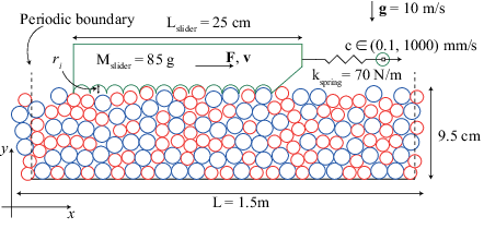
Figure 1: Granular simulation set-up (drawing not to scale). The discs represent the bulk sample with length LL and periodicity along xx.

Our slider-substrate setup is created in accordance with the experiment detailed in Zadeh et al. 2019b. In our two-dimensional simulation the substrate granular disks are sheared using a (rigid) slider of length Lslider=25​c​mL_{\text{slider}}=25\penalty\ cm and mass Mslider=8.5×10⁻²​k​gM_{\text{slider}}=8.5\times 10^{-2}\penalty\ kg. A spring of stiffness kspring=70​N/mk_{\text{spring}}=70\penalty\ N/m is attached to the slider, the free end of the spring is pulled at constant speed cc. To minimize the rotation of the slider due to spring vibrations and uniformly distribute the force due to pulling along the entire length, the spring is anchored to the middle of the slider. A schematic drawing of this setup is shown in Fig. 1.

To model this setup numerically Discrete Elements (DE) approach in LAMMPS Plimpton 1995 is chosen which considers each particle in the simulation as an individual element with a constant mass and radius. Furthermore, elements of this setup are fixed along the zz-axis hence behaves as two dimensional. Substrate discs, total of N=7770N=7770, are distributed bi-dispersedly with size ratio of Rb/Rs=1.25R_{b}/R_{s}=1.25 and number ratio Nb/Ns=2.5N_{b}/N_{s}=2.5. Here Nb⁡(s)N_{b(s)} and Rb⁡(s)R_{b(s)} denote the number of discs and their radii, respectively, we set Rb=2.5​m​mR_{b}=2.5\penalty\ mm for the larger disks. The density of substrate particles is constant at ρ=2.5×10⁴​k​g/m3\rho=2.5\times 10^{4}\penalty\ kg/m^{3}, which defines the mass of the particle mm. Gravity, acceleration of 10​m/s210\penalty\ m/s^{2}, is acting downwards on the entire system. The interaction between particles is modelled to have normal, tangential, and rolling forces, input parameters of these interactions are detailed in the next subsection.

As shown in Fig. 1, the rigid slider for this simulation has circular grooves with radius ri=2.5​m​mr_{i}=2.5\penalty\ mm on the base to induce additional friction. To setup the substrate, particles are initially dropped under gravity in the simulation box of length, L=1.5L=1.5 m, filled up to height of 0.3​L0.3L, which has periodic boundaries along xx. The slider is dropped on substrate particles after the (scaled) kinetic energy of the system is lower than K=∑i=1Nmi​𝐯i.𝐯j/2​N<10−10​JK=\sum_{i=1}^{N}m_{i}\mathbf{v}_{i}.\mathbf{v}_{j}/2N<10^{-10}\penalty\ J. The spring is attached once the slider comes to full stop above the substrate. The whole system is allowed to relax, such that particles and slider are completely at rest before shearing begins.

II.2 Mechanics of DE

Refer to caption
Figure 2: Interaction forces due to contact of particles (drawing not to scale).

The substrate disks are modelled as granular particles, for which the forces are updated at each timestep based on their interaction with one another, the slider and the walls. The parameters defined for interacting forces within the substrate and between the slider and the granular disks, discussed throughout this subsection, are outlined in Table 1.

The ii-th and jj-th particles in Fig. 2 with position vectors 𝐫i\mathbf{r}_{i} and 𝐫j\mathbf{r}_{j} only interact when the overlap δi​j=Ri+Rj−|𝐫i​j|>0\delta_{ij}=R_{i}+R_{j}-\left|\mathbf{r}_{ij}\right|>0 with 𝐫i​j=𝐫i−𝐫j\mathbf{r}_{ij}=\mathbf{r}_{i}-\mathbf{r}_{j}. The normal contact force is modelled as Hertz interaction, with the stiffness knk_{n}, and is calculated for each timestep as

𝐅n=−kn​Reff1/2​δi​j3/2​𝐧,\mathbf{F}_{n}=-k_{n}R^{1/2}_{\text{eff}}\delta^{3/2}_{ij}\mathbf{n}, (1)

with the effective radius Reff=Ri​Rj/(Ri+Rj)R_{\text{eff}}={R_{i}R_{j}}/(R_{i}+R_{j}) and the unit normal vector 𝐧=𝐫i​j/|𝐫i​j|\mathbf{n}={\mathbf{r}_{ij}}/{\left|\mathbf{r}_{ij}\right|}.

The tangential force 𝐅t\mathbf{F}_{t} between substrate particles is given by

𝐅t=−min⁡(μt​|𝐅n|,|−kt​𝝃t+𝐅tdamp|)​𝐭,\mathbf{F}_{t}=-\min(\penalty\ \mu_{t}\penalty\ |\mathbf{F}_{n}|,\penalty\ |-k_{t}\bm{\xi}_{t}+\mathbf{F}_{t}^{\text{damp}}|)\penalty\ \mathbf{t}, (2)

where μt\mu_{t} is the tangential friction coefficient, ktk_{t} is tangential stiffness of particles, 𝝃t=∫Tcont𝐯trel​(τ)​𝑑τ\bm{\xi}_{t}=\int_{T_{\text{cont}}}\mathbf{v}_{t}^{\text{rel}}(\tau)\penalty\ d\tau is the tangential displacement accumulated during the entire duration of the contact TcontT_{\text{cont}}, and 𝐭=𝐯trel/|𝐯trel|\mathbf{t}={\mathbf{v}_{t}^{\text{rel}}}/{\left|\mathbf{v}_{t}^{\text{rel}}\right|} is the tangential unit vector.

Damping is evaluated using a viscoelastic damping model in LAMMPS, the normal (tangential) component of which is calculated by

𝐅n⁡(t)damp=−ηn⁡(t)​𝐯n⁡(t)rel.\mathbf{F}_{n(t)}^{\text{damp}}=-\eta_{n(t)}\mathbf{v}_{n(t)}^{\text{rel}}. (3)

The normal damping coefficient ηn\eta_{n} is given by

ηn=a​ηn​0​meff,\eta_{n}=a\penalty\ \eta_{n0}\penalty\ m_{\text{eff}}, (4)

with the damping prefactor ηn​0\eta_{n0}, the radius of the contact area a=Reff​δi​ja=\sqrt{R_{\text{eff}}\penalty\ \delta_{ij}}, and the effective mass meff=mi​j/(mi+mj)m_{\text{eff}}={m_{ij}}/{(m_{i}+m_{j})}. We have ηt∝ηn\eta_{t}\propto\eta_{n} with the proportionality factor xγ​tx_{\gamma t}. The normal relative velocity vector is 𝐯nrel=(𝐯rel⋅𝐧)​𝐧\mathbf{v}_{n}^{\text{rel}}=(\mathbf{v}_{\text{rel}}\cdot\mathbf{n})\penalty\ \mathbf{n} where 𝐯rel=𝐯i−𝐯j\mathbf{v}_{\text{rel}}=\mathbf{v}_{i}-\mathbf{v}_{j}. We define the relative tangential velocity 𝐯trel\mathbf{v}_{t}^{\text{rel}} as

𝐯trel=𝐯t−(Ri​θ˙i+Rj​θ˙j)​𝐞z×𝐧,\mathbf{v}_{t}^{\text{rel}}=\mathbf{v}_{t}-\left(R_{i}\dot{\theta}_{i}+R_{j}\dot{\theta}_{j}\right)\mathbf{e}_{z}\times\mathbf{n}, (5)

with the angular velocity θ˙i​𝐞𝐳\dot{\theta}_{i}\mathbf{e_{z}} of the ii-th particle.

Rolling force during a contact is

𝐅r=−min⁡(μr​|𝐅n|,|−kr​𝝃r−γr​𝐯r|)​𝐤,\mathbf{F}_{r}=-\min(\penalty\ \mu_{r}|\mathbf{F}_{n}|,\left|-k_{r}\bm{\xi}_{r}-\gamma_{r}\mathbf{v}_{r}\right|)\penalty\ \mathbf{k}, (6)

where μr\mu_{r} is the rolling friction, krk_{r} is rolling stiffness, γr\gamma_{r} is the rolling dampness, 𝐯r=Reff​(θ˙i−θ˙j)​𝐞z×𝐧\mathbf{v}_{r}=R_{\text{eff}}\left(\dot{\theta}_{i}-\dot{\theta}_{j}\right)\mathbf{e}_{z}\times\mathbf{n} is the relative rolling velocity, 𝝃r=∫T𝐯r​(τ)​𝑑τ\bm{\xi}_{r}=\int_{T}\mathbf{v}_{r}(\tau)d\tau is rolling displacement, and 𝐤=𝐯r/|𝐯r|\mathbf{k}=\mathbf{v}_{r}/|\mathbf{v}_{r}|.

Parameter Symbol Type ia Type iib Units
Normal stiffness knk_{n} 1×1061\times 10^{6} 1×1061\times 10^{6} N/m2{N/m}^{2}
Normal damping ηn​0\eta_{n0} 5×1055\times 10^{5} 5×1055\times 10^{5} 1/m⋅s1/{m}\cdot\text{s}
Tangential stiffness ktk_{t} 1×10¹¹\times 10^{1} 1×1001\times 10^{0} N/m{N/m}
Sliding friction μt\mu_{t} 1×10¹¹\times 10^{1} 1×1001\times 10^{0} -
Damping ratio xγ​tx_{\gamma t} 1×10¹¹\times 10^{1} 1×1041\times 10^{4} -
Rolling friction μr\mu_{r} 1×10¹¹\times 10^{1} 00 -
Rolling stiffness krk_{r} 1×10¹¹\times 10^{1} 00 N/m{N/m}
Rolling damping γr\gamma_{r} 1×1041\times 10^{4} 00 k​g/skg/s
  • a

    Substrate/Substrate

  • b

    Slider/Substrate

Table 1: Microscopic material parameters used for the granular model.

Newton’s equations of motion, updated every timestep, are

mi​𝐫¨i\displaystyle m_{i}\ddot{\mathbf{r}}_{i} =\displaystyle= 𝐅n+𝐅ndamp+𝐅t+mi​𝐠,\displaystyle\mathbf{F}_{n}+\mathbf{F}_{n}^{\text{damp}}+\mathbf{F}_{t}+m_{i}\mathbf{g},
mi​Ri2​θ¨i​𝐞z\displaystyle m_{i}R^{2}_{i}\ddot{\theta}_{i}\mathbf{e}_{z} =\displaystyle= Ri​𝐧×(𝐅t+𝐅r).\displaystyle R_{i}\penalty\ \mathbf{n}\times(\mathbf{F}_{t}+\mathbf{F}_{r}). (7)

The rate unit (inverse timescale) is set by gravity g/Rs\sqrt{{g}/{R_{s}}}. The normal vibrational frequency is defined as ωn=kneff/meff\omega_{n}=\sqrt{k^{\text{eff}}_{n}/m^{\text{eff}}} with kneff=a​knk^{\text{eff}}_{n}=ak_{n}. For the example of normal force, our choice of microscopic parameters obeys the following separation of timescales

ωn≫gRs≫cRs.\omega_{n}\gg\sqrt{\frac{g}{R_{s}}}\gg\frac{c}{R_{s}}. (8)

This leads to an internal dynamics reasonably close to the experimental setting. We also set the discretization time Δ​t=0.05​ωn−1\Delta t=0.05\penalty\ \omega_{n}^{-1}. Furthermore, the dissipation rate τd−1=a​ηn​0\tau^{-1}_{d}=a\eta_{n0}, of our simulations relates to the vibrations frequency as τd−1/ωn≃0.2\tau^{-1}_{d}/\omega_{n}\simeq 0.2, to recover damped dynamics where the damping rates are such that they reproduce experimental observations.

Refer to caption
Refer to caption
Figure 3: Force response f⁡(t)f(t) and slider speed v⁡(t)v(t) (normalized to the pulling speed cc) plotted against tt at a) c=0.1c=0.1 mm/s b) c=1000c=1000 mm/s.
\begin{overpic}[PSDc0.1.eps] \centering\hbox to99.05pt{\vbox to92.98pt{\pgfpicture\makeatletter\hbox{\hskip 4.33997pt\lower-3.63857pt\hbox to0.0pt{\lxSVG@begingroup@{_scopebegin} \lxSVG@begingroup@{stroke} \lxSVG@begingroup@{fill} \lxSVG@setlinewidth{\the\pgflinewidth}\lxSVG@begingroup@{stroke-width} \lx@inpgf@ignorespaces\nullfont\hbox to0.0pt{\lxSVG@begingroup@{_scopebegin} {}{{\lx@inpgf@ignorespaces}}\lx@inpgf@ignorespaces\hbox{\hbox{{\lxSVG@begingroup@{_scopebegin} {{}{{}}{}{}} \lxSVG@closescope }}} {{}}{{}}\lx@inpgf@ignorespaces\hbox{\hbox{{\lxSVG@begingroup@{_scopebegin} \color[rgb]{1,1,1}{{}{}{{ {}{}}}{ {}{}} {{}{{\lx@inpgf@ignorespaces}}}{{}{\lx@inpgf@ignorespaces}}{}{{}{\lx@inpgf@ignorespaces}} {\lxSVG@begingroup@{_scopebegin} \color[rgb]{1,1,1}\lx@inpgf@ignorespaces \lxSVG@closescope }{{{{\lx@inpgf@ignorespaces}}\lxSVG@begingroup@{_scopebegin} \lxSVG@transformcm{1.0}{0.0}{0.0}{1.0}{-1.00696pt}{-0.30556pt}\lxSVG@begingroup@{transform} \pgfsys@hbox{66}\lxSVG@closescope }}} \lxSVG@closescope }}} {}{{\lx@inpgf@ignorespaces}}\lx@inpgf@ignorespaces\hbox{\hbox{{\lxSVG@begingroup@{_scopebegin} {{}{{}}{}{}} \lxSVG@closescope }}} {{{}{}{}{}{}{}{}{}{}{}}{{}{}{}{}{}{}{}{}{}{}{}{}{}{}{}{}{}{}{}{}{}{}{}{}{}{}{}{}{}{}{}{}{}{}{}{}{}{}{}{}{}{}{}{}{}{}}{{}{}{}{}{}}}{{{}{}{}{}{}{}{}{}{}{}}{{}{}{}{}{}{}{}{}{}{}{}{}{}{}{}{}{}{}{}{}{}{}{}{}{}{}{}{}{}{}{}{}{}{}{}{}{}{}{}{}{}{}{}{}{}{}}{{}{}{}{}{}}}{{{}{}{}{}{}}}{{{}{}{}{}{}}}{{}}{}{}{}{{\lx@inpgf@ignorespaces}}\lx@inpgf@ignorespaces\hbox{\hbox{{\lxSVG@begingroup@{_scopebegin} {{}{{}}{}{}} \lxSVG@closescope }}} {{}}{}{}{}{{\lx@inpgf@ignorespaces}}\lx@inpgf@ignorespaces\hbox{\hbox{{\lxSVG@begingroup@{_scopebegin} {{}{{}}{}{}} \lxSVG@closescope }}} {{{}{}{}{}{}{}{}{}{}{}}{{}{}{}{}{}{}{}{}{}{}}}{{}}{}{}{}{{\lx@inpgf@ignorespaces}}\lx@inpgf@ignorespaces\hbox{\hbox{{\lxSVG@begingroup@{_scopebegin} {{}{{}}{}{}} \lxSVG@closescope }}} {{}}{}{}{}{{}}\lx@inpgf@ignorespaces\hbox{\hbox{{\lxSVG@begingroup@{_scopebegin} {{}{}{{ {}{}}}{ {}{}} {{}{{\lx@inpgf@ignorespaces}}}{{}{\lx@inpgf@ignorespaces}}{}{{}{\lx@inpgf@ignorespaces}} {\lx@inpgf@ignorespaces }{{{{\lx@inpgf@ignorespaces}}\lxSVG@begingroup@{_scopebegin} \lxSVG@transformcm{1.0}{0.0}{0.0}{1.0}{65.50873pt}{80.2572pt}\lxSVG@begingroup@{transform} \pgfsys@hbox{66}\lxSVG@closescope }}} \lxSVG@closescope }}} {{}}{}{}{}{{}}\lx@inpgf@ignorespaces\hbox{\hbox{{\lxSVG@begingroup@{_scopebegin} {{}{}{{ {}{}}}{ {}{}} {{}{{\lx@inpgf@ignorespaces}}}{{}{\lx@inpgf@ignorespaces}}{}{{}{\lx@inpgf@ignorespaces}} {\lx@inpgf@ignorespaces }{{{{\lx@inpgf@ignorespaces}}\lxSVG@begingroup@{_scopebegin} \lxSVG@transformcm{1.0}{0.0}{0.0}{1.0}{83.36507pt}{70.15356pt}\lxSVG@begingroup@{transform} \pgfsys@hbox{66}\lxSVG@closescope }}} \lxSVG@closescope }}} {{}}{}{{}}{}{{}} {}{}\lxSVG@begingroup@{_scopebegin} \color[rgb]{0,0,0}\lxSVG@setlinewidth{\the\pgflinewidth}\lxSVG@begingroup@{stroke-width} \lx@inpgf@ignorespaces{}\lxSVG@stroke\lxSVG@drawpath@unclipped{M 105.37 104.92 L 105.37 123.43}{fill:none} \lx@inpgf@ignorespaces \lxSVG@closescope {{}}{}{{}}{}{{}} {}{}\lxSVG@begingroup@{_scopebegin} \color[rgb]{0,0,0}\lxSVG@setlinewidth{\the\pgflinewidth}\lxSVG@begingroup@{stroke-width} \lx@inpgf@ignorespaces{}\lxSVG@stroke\lxSVG@drawpath@unclipped{M 105.37 104.92 L 130.85 104.92}{fill:none} \lx@inpgf@ignorespaces \lxSVG@closescope {{}}{}{{}}{}{{}} {}{}\lxSVG@begingroup@{_scopebegin} \color[rgb]{0,0,0}\lxSVG@setlinewidth{\the\pgflinewidth}\lxSVG@begingroup@{stroke-width} \lx@inpgf@ignorespaces{}\lxSVG@stroke\lxSVG@drawpath@unclipped{M 105.37 123.43 L 130.85 104.92}{fill:none} \lx@inpgf@ignorespaces \lxSVG@closescope \lxSVG@closescope {\lx@inpgf@ignorespaces}{\lx@inpgf@ignorespaces}{\lx@inpgf@ignorespaces}\hss}\lxSVG@discardpath\lxSVG@closescope \hss}}\lxSVG@closescope\endpgfpicture}} \par \@add@centering\end{overpic}
Refer to caption
Figure 4: Power spectrum |f¯​(ω)|2|\bar{f}(\omega)|^{2} associated with the force timeseries at a) c=0.1c=0.1 mm/s b) c=1000c=1000 mm/s. The inset for b) is the same as the main plot but on the lin-lin scale. The dashed line for a) denotes |f¯​(ω)|2∝ω−δ|\bar{f}(\omega)|^{2}\propto\omega^{-\delta} with δ=2.2\delta=2.2. The solid curves correspond to the binned data.

III Stick-slip dynamics vs. stable sliding

We performed a series of tests on samples with different pulling speeds cc. The magnitude of the resulting force 𝐅\mathbf{F} and velocity of the slider 𝐯\mathbf{v} scaled by cc are plotted against time in Fig. 3. At the slowest rate c=0.1c=0.1 mm/s, the response is characterized by abrupt force drops preceded by longer stress build-up periods as in Fig. 3(a). Similarly, the slider velocity exhibits a stick-slip dynamics with quiescent periods that are frequently interrupted by short-lived active phases. By contrast, Fig. 3(b), corresponding to c=1000c=1000 mm/s, shows a well-established quasi-periodic sliding regime. Both dynamical behaviors are in agreement with experimental observations Zadeh et al. 2019a; Zadeh et al. 2019b; Cheng et al..

In frequency domain ω\omega, the stick-slip dynamics at the low driving rate is marked by a scale free power law behavior associated with the power spectral density of the force signal |f¯​(ω)|2|\bar{f}(\omega)|^{2} as displayed in Fig. 4(a). We find |f¯​(ω)|2∝ω−δ|\bar{f}(\omega)|^{2}\propto\omega^{-\delta} with δ≃2.2\delta\simeq 2.2 over at least four decades in ω\omega. This is in close agreement with the measured exponent corresponding to the experimental setup with δ=2.4±0.2\delta=2.4\pm 0.2, where the power law extended over a shorter range of frequencies Zadeh et al. 2019b. In Fig. 4(b), the power spectrum associated with the faster driving rate at c=1000c=1000 mm/s develops a characteristic peak at ω≃5​H​z\omega\simeq 5\penalty\ Hz which is a signature of the quasi-periodic signal in the time domain. As reported in the experimental setting Zadeh et al. 2019b, this characteristic frequency should scale with the driving rate cc and differ from the natural frequency set by the slider mass MsliderM_{\text{slider}} and (pulling) spring constant kspringk_{\text{spring}}, i.e. ω2=kspring/Mslider\omega^{2}=k_{\text{spring}}/M_{\text{slider}}. It should be noted that the driving rate in Fig. 4(b) is a factor of 10 larger than the fastest case reported in the experiment which leads to a more pronounced peak in the frequency domain.

IV “Seimicity” analysis

In this section, we investigate the properties of the stick-slip events of the slider, often denoted as avalanches. Specifically, we probe the dissipated energy power and its evolution with time to define the size and duration of individual avalanches. This allows us to quantify the avalanche size statistics along with inter-occurrence time distributions both showing non-trivial scaling features at low driving rates. Other statistical measures such as productivity relation or temporal aftershock rates require a proper identification of mainshock-aftershocks sequences which will be discussed in subsequent sections.

Figure 5: a) Definition of the avalanche size SS, avalanche duration TT, avalanche inter-occurrence time τ\tau, and slider rest time τw\tau_{w} at c=0.1​m​m/sc=0.1\penalty\ mm/s. The main plot is a magnified view of the power time series shown in the inset. b) Magnitude time series.
Refer to caption
Refer to caption
\begin{overpic}[PDFEventSize.eps] \centering\hbox to157.67pt{\vbox to248.31pt{\pgfpicture\makeatletter\hbox{\hskip 4.33997pt\lower-3.63857pt\hbox to0.0pt{\lxSVG@begingroup@{_scopebegin} \lxSVG@begingroup@{stroke} \lxSVG@begingroup@{fill} \lxSVG@setlinewidth{\the\pgflinewidth}\lxSVG@begingroup@{stroke-width} \lx@inpgf@ignorespaces\nullfont\hbox to0.0pt{\lxSVG@begingroup@{_scopebegin} {}{{\lx@inpgf@ignorespaces}}\lx@inpgf@ignorespaces\hbox{\hbox{{\lxSVG@begingroup@{_scopebegin} {{}{{}}{}{}} \lxSVG@closescope }}} {{}}{{}}\lx@inpgf@ignorespaces\hbox{\hbox{{\lxSVG@begingroup@{_scopebegin} \color[rgb]{1,1,1}{{}{}{{ {}{}}}{ {}{}} {{}{{\lx@inpgf@ignorespaces}}}{{}{\lx@inpgf@ignorespaces}}{}{{}{\lx@inpgf@ignorespaces}} {\lxSVG@begingroup@{_scopebegin} \color[rgb]{1,1,1}\lx@inpgf@ignorespaces \lxSVG@closescope }{{{{\lx@inpgf@ignorespaces}}\lxSVG@begingroup@{_scopebegin} \lxSVG@transformcm{1.0}{0.0}{0.0}{1.0}{-1.00696pt}{-0.30556pt}\lxSVG@begingroup@{transform} \pgfsys@hbox{66}\lxSVG@closescope }}} \lxSVG@closescope }}} {}{{\lx@inpgf@ignorespaces}}\lx@inpgf@ignorespaces\hbox{\hbox{{\lxSVG@begingroup@{_scopebegin} {{}{{}}{}{}} \lxSVG@closescope }}} {{{}{}{}{}{}{}{}{}{}{}}{{}{}{}{}{}{}{}{}{}{}{}{}{}{}{}{}{}{}{}{}{}{}{}{}{}{}{}{}{}{}{}{}{}{}{}{}{}{}{}{}{}{}{}{}{}{}}{{}{}{}{}{}{}{}{}{}{}}{{}{}{}{}{}}}{{{}{}{}{}{}{}{}{}{}{}}{{}{}{}{}{}{}{}{}{}{}{}{}{}{}{}{}{}{}{}{}{}{}{}{}{}{}{}{}{}{}{}{}{}{}{}{}{}{}{}{}{}{}{}{}{}{}}{{}{}{}{}{}{}{}{}{}{}}{{}{}{}{}{}}}{{{}{}{}{}{}}}{{{}{}{}{}{}}}{{}}{}{}{}{{\lx@inpgf@ignorespaces}}\lx@inpgf@ignorespaces\hbox{\hbox{{\lxSVG@begingroup@{_scopebegin} {{}{{}}{}{}} \lxSVG@closescope }}} {{}}{}{}{}{{\lx@inpgf@ignorespaces}}\lx@inpgf@ignorespaces\hbox{\hbox{{\lxSVG@begingroup@{_scopebegin} {{}{{}}{}{}} \lxSVG@closescope }}} {{{}{}{}{}{}{}{}{}{}{}}{{}{}{}{}{}{}{}{}{}{}}}{{}}{}{}{}{{\lx@inpgf@ignorespaces}}\lx@inpgf@ignorespaces\hbox{\hbox{{\lxSVG@begingroup@{_scopebegin} {{}{{}}{}{}} \lxSVG@closescope }}} {{}}{}{}{}{{}}\lx@inpgf@ignorespaces\hbox{\hbox{{\lxSVG@begingroup@{_scopebegin} {{}{}{{ {}{}}}{ {}{}} {{}{{\lx@inpgf@ignorespaces}}}{{}{\lx@inpgf@ignorespaces}}{}{{}{\lx@inpgf@ignorespaces}} {\lx@inpgf@ignorespaces }{{{{\lx@inpgf@ignorespaces}}\lxSVG@begingroup@{_scopebegin} \lxSVG@transformcm{1.0}{0.0}{0.0}{1.0}{63.93675pt}{225.36691pt}\lxSVG@begingroup@{transform} \pgfsys@hbox{66}\lxSVG@closescope }}} \lxSVG@closescope }}} {{}}{}{}{}{{}}\lx@inpgf@ignorespaces\hbox{\hbox{{\lxSVG@begingroup@{_scopebegin} {{}{}{{ {}{}}}{ {}{}} {{}{{\lx@inpgf@ignorespaces}}}{{}{\lx@inpgf@ignorespaces}}{}{{}{\lx@inpgf@ignorespaces}} {\lx@inpgf@ignorespaces }{{{{\lx@inpgf@ignorespaces}}\lxSVG@begingroup@{_scopebegin} \lxSVG@transformcm{1.0}{0.0}{0.0}{1.0}{73.71637pt}{236.82858pt}\lxSVG@begingroup@{transform} \pgfsys@hbox{66}\lxSVG@closescope }}} \lxSVG@closescope }}} {{}}{}{{}}{}{{}} {}{}\lxSVG@begingroup@{_scopebegin} \color[rgb]{0,0,0}\lxSVG@setlinewidth{\the\pgflinewidth}\lxSVG@begingroup@{stroke-width} \lx@inpgf@ignorespaces{}\lxSVG@stroke\lxSVG@drawpath@unclipped{M 99.1 326.1 L 121.37 326.1}{fill:none} \lx@inpgf@ignorespaces \lxSVG@closescope {{}}{}{{}}{}{{}} {}{}\lxSVG@begingroup@{_scopebegin} \color[rgb]{0,0,0}\lxSVG@setlinewidth{\the\pgflinewidth}\lxSVG@begingroup@{stroke-width} \lx@inpgf@ignorespaces{}\lxSVG@stroke\lxSVG@drawpath@unclipped{M 99.1 326.1 L 99.1 303.83}{fill:none} \lx@inpgf@ignorespaces \lxSVG@closescope {{}}{}{{}}{}{{}} {}{}\lxSVG@begingroup@{_scopebegin} \color[rgb]{0,0,0}\lxSVG@setlinewidth{\the\pgflinewidth}\lxSVG@begingroup@{stroke-width} \lx@inpgf@ignorespaces{}\lxSVG@stroke\lxSVG@drawpath@unclipped{M 121.37 326.1 L 99.1 303.83}{fill:none} \lx@inpgf@ignorespaces \lxSVG@closescope {}{{\lx@inpgf@ignorespaces}}\lx@inpgf@ignorespaces\hbox{\hbox{{\lxSVG@begingroup@{_scopebegin} {{}{{}}{}{}} \lxSVG@closescope }}} {{{}{}{}{}{}{}{}{}{}{}}{{}{}{}{}{}{}{}{}{}{}{}{}{}{}{}{}{}{}{}{}{}{}{}{}{}{}{}{}{}{}{}{}{}{}{}{}{}{}{}{}{}{}{}{}{}{}}{{}{}{}{}{}{}}}{{{}{}{}{}{}{}{}{}{}{}}{{}{}{}{}{}{}{}{}{}{}{}{}{}{}{}{}{}{}{}{}{}{}{}{}{}{}{}{}{}{}{}{}{}{}{}{}{}{}{}{}{}{}{}{}{}{}}{{}{}{}{}{}{}}}{{{}{}{}{}{}}}{{{}{}{}{}{}}}{{}}{}{}{}{{\lx@inpgf@ignorespaces}}\lx@inpgf@ignorespaces\hbox{\hbox{{\lxSVG@begingroup@{_scopebegin} {{}{{}}{}{}} \lxSVG@closescope }}} {{}}{}{}{}{{\lx@inpgf@ignorespaces}}\lx@inpgf@ignorespaces\hbox{\hbox{{\lxSVG@begingroup@{_scopebegin} {{}{{}}{}{}} \lxSVG@closescope }}} {{{}{}{}{}{}{}{}{}{}{}}{{}{}{}{}{}{}{}{}{}{}}}{{}}{}{}{}{{\lx@inpgf@ignorespaces}}\lx@inpgf@ignorespaces\hbox{\hbox{{\lxSVG@begingroup@{_scopebegin} {{}{{}}{}{}} \lxSVG@closescope }}} {{}}{}{}{}{{}}\lx@inpgf@ignorespaces\hbox{\hbox{{\lxSVG@begingroup@{_scopebegin} {{}{}{{ {}{}}}{ {}{}} {{}{{\lx@inpgf@ignorespaces}}}{{}{\lx@inpgf@ignorespaces}}{}{{}{\lx@inpgf@ignorespaces}} {\lx@inpgf@ignorespaces }{{{{\lx@inpgf@ignorespaces}}\lxSVG@begingroup@{_scopebegin} \lxSVG@transformcm{1.0}{0.0}{0.0}{1.0}{138.0889pt}{94.48367pt}\lxSVG@begingroup@{transform} \pgfsys@hbox{66}\lxSVG@closescope }}} \lxSVG@closescope }}} {{}}{}{}{}{{}}\lx@inpgf@ignorespaces\hbox{\hbox{{\lxSVG@begingroup@{_scopebegin} {{}{}{{ {}{}}}{ {}{}} {{}{{\lx@inpgf@ignorespaces}}}{{}{\lx@inpgf@ignorespaces}}{}{{}{\lx@inpgf@ignorespaces}} {\lx@inpgf@ignorespaces }{{{{\lx@inpgf@ignorespaces}}\lxSVG@begingroup@{_scopebegin} \lxSVG@transformcm{1.0}{0.0}{0.0}{1.0}{128.89018pt}{106.48717pt}\lxSVG@begingroup@{transform} \pgfsys@hbox{66}\lxSVG@closescope }}} \lxSVG@closescope }}} {{}}{}{{}}{}{{}} {}{}\lxSVG@begingroup@{_scopebegin} \color[rgb]{0,0,0}\lxSVG@setlinewidth{\the\pgflinewidth}\lxSVG@begingroup@{stroke-width} \lx@inpgf@ignorespaces{}\lxSVG@stroke\lxSVG@drawpath@unclipped{M 191.43 145.74 L 191.43 121.97}{fill:none} \lx@inpgf@ignorespaces \lxSVG@closescope {{}}{}{{}}{}{{}} {}{}\lxSVG@begingroup@{_scopebegin} \color[rgb]{0,0,0}\lxSVG@setlinewidth{\the\pgflinewidth}\lxSVG@begingroup@{stroke-width} \lx@inpgf@ignorespaces{}\lxSVG@stroke\lxSVG@drawpath@unclipped{M 191.43 145.74 L 170.77 145.74}{fill:none} \lx@inpgf@ignorespaces \lxSVG@closescope {{}}{}{{}}{}{{}} {}{}\lxSVG@begingroup@{_scopebegin} \color[rgb]{0,0,0}\lxSVG@setlinewidth{\the\pgflinewidth}\lxSVG@begingroup@{stroke-width} \lx@inpgf@ignorespaces{}\lxSVG@stroke\lxSVG@drawpath@unclipped{M 191.43 121.97 L 170.77 145.74}{fill:none} \lx@inpgf@ignorespaces \lxSVG@closescope \lxSVG@closescope {\lx@inpgf@ignorespaces}{\lx@inpgf@ignorespaces}{\lx@inpgf@ignorespaces}\hss}\lxSVG@discardpath\lxSVG@closescope \hss}}\lxSVG@closescope\endpgfpicture}} \@add@centering\end{overpic}
Figure 6: a) Scatter plot of the avalanche duration TT vs. avalanche size SS, b) avalanche size distributions, both at c=0.1​m​m/sc=0.1\penalty\ mm/s. The symbols in a) indicate the mean duration T¯\bar{T} over prescribed bins in SS. The dashdotted line in a) indicates a power law T∝S1/γT\propto S^{1/\gamma} with γ=1.2\gamma=1.2. The dashdotted line in b) is a guide to the power law P⁡(S)∝S−βP(S)\propto S^{-\beta} with β=1.5\beta=1.5. The error bars denote one standard error. The inset is the same as the main plot but rescaled by SβS^{\beta}.

IV.1 Avalanche Statistics

We define the spontaneous rate of dissipated energy of the slider as U˙=𝐅⋅𝐯\dot{U}=\mathbf{F}\cdot\mathbf{v} during the slip period. The power signal is shown in Fig. 5(a) with a noise floor U˙c≃10−6\dot{U}_{c}\simeq 10^{-6} that is intermittently interrupted by short-lived stick-slip events or avalanches. Figure 5(b) displays the timeseries associated with the avalanche size S=∫titi+Ti{U˙​(t)−Uc˙}​𝑑tS=\int_{t_{i}}^{t_{i}+T_{i}}\{\dot{U}(t)-\dot{U_{c}}\}\penalty\ dt which has dimensions of energy and corresponds to an avalanche initiated at tit_{i} with duration TiT_{i}.

Figure 6 displays the scatter plot of the avalanche size SS and event duration TT along with the avalanche size distributions P⁡(S)P(S). The scatter plot in Fig. 6(a) demonstrates that, statistically speaking, larger avalanches tend to have longer duration with a scaling behavior that may be described on average as T∝S1/γT\propto S^{1/\gamma} with γ≃1.2\gamma\simeq 1.2, in agreement with the experimental observation Zadeh et al. 2019a. The scaling regime spans almost three decades in SS before reaching a plateau at large avalanche sizes. The avalanche size distribution in Fig. 6(b) decays as a power-law P⁡(S)∝S−βP(S)\propto S^{-\beta} over at least three decades above a (lower) cut-off size Smin≃10−6S_{\text{min}}\simeq 10^{-6} with β≃1.5\beta\simeq 1.5 which is within the range of measured exponents in experiments 1.2−1.71.2-1.7 Lherminier et al. 2019; Zadeh et al. 2019a and matches the mean-field estimate β=3/2\beta=3/2 Fisher 1998. In all of the subsequent avalanche analyses, we use Smin=10−6S_{\text{min}}=10^{-6} as a lower bound for event size thresholds, e.g. Sc≥SminS_{c}\geq S_{\text{min}}, to ensure a meaningful (power-law) scaling regime associated with SS.

The avalanche size distribution can be expressed in an accumulated form as P⁡(size>S)=(Smin/S)β−1P(\text{size}>S)=(S_{\text{min}}/S)^{\beta-1}. This distribution may also be transformed into the classical Gutenberg-Richter magnitude-frequency relation P⁡(mag.>m)=10−b⁡(m−mc)P(\text{mag.}>m)=10^{-b(m-m_{c})} with magnitude of completeness mcm_{c} and b−b-value that controls the exponential decay rate. The magnitude mm is empirically related to seismic moment MM via m=c0​log10​M−c1m=c_{0}\text{log}_{10}M-c_{1} with non-universal parameters c0c_{0} and c1c_{1} Kagan 2013. From this relationship, it follows that b=(βM−1)/c0b=(\beta_{M}-1)/c_{0} with exponent βM\beta_{M} describing the power-law decay of seismic moments distributions de Arcangelis et al. 2016. It should be noted that we measure the dissipated energy SS, not the seismic moment MM with the latter typically evaluated based on the shear modulus, slip size, and associated stress drop. Provided that SS is proportional to MM (see de Arcangelis et al. 2016; Lord-May et al. 2020 and references therein for a discussion of this assumption), one obtains β=βM\beta=\beta_{M}. Using c0=23c_{0}=\frac{2}{3} established for large earthquakes de Arcangelis et al. 2016, we obtain b≃0.75b\simeq 0.75 which is smaller than the commonly observed b≈1b\approx 1 in tectonic settings, though there is some variability across different settings Schorlemmer et al. 2005; Gu et al. 2013; Scholz 2015; Davidsen and Baiesi 2016. One could, however, dispute the conversion of β\beta to bb-value for our small avalanche sizes here Ben-Zion and Zhu 2002; Lord-May et al. 2020, such that a direct comparison with tectonic seismicity might not be appropriate.

\begin{overpic}[Friction.eps] \centering\hbox to8.68pt{\vbox to7.28pt{\pgfpicture\makeatletter\hbox{\hskip 4.33997pt\lower-3.63857pt\hbox to0.0pt{\lxSVG@begingroup@{_scopebegin} \lxSVG@begingroup@{stroke} \lxSVG@begingroup@{fill} \lxSVG@setlinewidth{\the\pgflinewidth}\lxSVG@begingroup@{stroke-width} \lx@inpgf@ignorespaces\nullfont\hbox to0.0pt{\lxSVG@begingroup@{_scopebegin} {}{{\lx@inpgf@ignorespaces}}\lx@inpgf@ignorespaces\hbox{\hbox{{\lxSVG@begingroup@{_scopebegin} {{}{{}}{}{}} \lxSVG@closescope }}} {{}}{{}}\lx@inpgf@ignorespaces\hbox{\hbox{{\lxSVG@begingroup@{_scopebegin} \color[rgb]{1,1,1}{{}{}{{ {}{}}}{ {}{}} {{}{{\lx@inpgf@ignorespaces}}}{{}{\lx@inpgf@ignorespaces}}{}{{}{\lx@inpgf@ignorespaces}} {\lxSVG@begingroup@{_scopebegin} \color[rgb]{1,1,1}\lx@inpgf@ignorespaces \lxSVG@closescope }{{{{\lx@inpgf@ignorespaces}}\lxSVG@begingroup@{_scopebegin} \lxSVG@transformcm{1.0}{0.0}{0.0}{1.0}{-1.00696pt}{-0.30556pt}\lxSVG@begingroup@{transform} \pgfsys@hbox{66}\lxSVG@closescope }}} \lxSVG@closescope }}} \lxSVG@closescope {\lx@inpgf@ignorespaces}{\lx@inpgf@ignorespaces}{\lx@inpgf@ignorespaces}\hss}\lxSVG@discardpath\lxSVG@closescope \hss}}\lxSVG@closescope\endpgfpicture}} \@add@centering\end{overpic}
Figure 7: Avalanche statistics at multiple inter-particle sliding friction μt\mu_{t} and rolling friction μr\mu_{r}. a) Avalanche duration TT plotted against event size SS. b) (non-normalized) avalanche size distribution P⁡(S)P(S). The first pair of parameters correspond to inter-particle friction and second one relates to the slider-substrate friction.
\begin{overpic}[Damping.eps] \centering\hbox to8.68pt{\vbox to7.28pt{\pgfpicture\makeatletter\hbox{\hskip 4.33997pt\lower-3.63857pt\hbox to0.0pt{\lxSVG@begingroup@{_scopebegin} \lxSVG@begingroup@{stroke} \lxSVG@begingroup@{fill} \lxSVG@setlinewidth{\the\pgflinewidth}\lxSVG@begingroup@{stroke-width} \lx@inpgf@ignorespaces\nullfont\hbox to0.0pt{\lxSVG@begingroup@{_scopebegin} {}{{\lx@inpgf@ignorespaces}}\lx@inpgf@ignorespaces\hbox{\hbox{{\lxSVG@begingroup@{_scopebegin} {{}{{}}{}{}} \lxSVG@closescope }}} {{}}{{}}\lx@inpgf@ignorespaces\hbox{\hbox{{\lxSVG@begingroup@{_scopebegin} \color[rgb]{1,1,1}{{}{}{{ {}{}}}{ {}{}} {{}{{\lx@inpgf@ignorespaces}}}{{}{\lx@inpgf@ignorespaces}}{}{{}{\lx@inpgf@ignorespaces}} {\lxSVG@begingroup@{_scopebegin} \color[rgb]{1,1,1}\lx@inpgf@ignorespaces \lxSVG@closescope }{{{{\lx@inpgf@ignorespaces}}\lxSVG@begingroup@{_scopebegin} \lxSVG@transformcm{1.0}{0.0}{0.0}{1.0}{-1.00696pt}{-0.30556pt}\lxSVG@begingroup@{transform} \pgfsys@hbox{66}\lxSVG@closescope }}} \lxSVG@closescope }}} \lxSVG@closescope {\lx@inpgf@ignorespaces}{\lx@inpgf@ignorespaces}{\lx@inpgf@ignorespaces}\hss}\lxSVG@discardpath\lxSVG@closescope \hss}}\lxSVG@closescope\endpgfpicture}} \@add@centering\end{overpic}
Figure 8: Avalanche statistics at multiple damping rates for both normal and rolling components ηn​0,γr\eta_{n0},\gamma_{r}. a) Avalanche duration TT versus event size SS b) (non-normalized) avalanche size distribution P⁡(S)P(S).

IV.1.1 Robustness Analysis

Figure 7 and 8 examine the overall robustness of our findings with respect to changes in the inter-particle (sliding and rolling) friction coefficient as well as the (normal and rolling) dissipation time scales. Displayed in Fig. 7(a), the scaling relation between avalanche size and duration remains almost insensitive to variations in the microscopic friction. The avalanche size exponent β\beta seems to be also a robust scaling feature at larger SS values as shown in Fig. 7(b). Higher damping rates in Fig. 8(a) lead to an overall shift in the avalanche duration but has no discernible effect on exponent γ\gamma within the scaling regime at small and intermediate SS. This is also true for size distributions in Fig. 8(b) where β≃1.5\beta\simeq 1.5 seems to be a robust scaling exponent.

In order to probe potential effects of the surface roughness of the slider on the avalanche statistics, we considered different cases of depths of the grooves at the base of the slider on the granular substrate. We find that there are no considerable effect on the overall avalanche statistics (see Fig. A3 ). In particular, the power-law exponents are unaltered indicating that the variation in the interaction between the slider and the substrate do not affect the universality class. Similarly, changes in polydispersity (see Fig. A2) do not lead to any quantitative changes between the different sets of avalanche size and duration distributions.

IV.2 Avalanche Inter-occurrence Time and Slider Rest Time Statistics

For a homogeneous Poisson process with independent events of constant rate λ\lambda, the inter-occurrence time statistics should obey an exponential distribution P⁡(τ)=λ​e−λ​τP(\tau)=\lambda e^{-\lambda\tau} with τi=ti−ti−1\tau_{i}=t_{i}-t_{i-1} denoting the time interval between two consecutive avalanches, i.e., the time interval between the onset of avalanche i−1i-1 and the onset of avalanche ii (see Fig. 5(a)). Deviations from this exponential distribution are demonstrated in Fig. 9(a) where the rescaled distributions τ¯​P​(τ)\bar{\tau}P(\tau) are plotted against τ/τ¯\tau/\bar{\tau} for avalanches of sizes S>ScS>S_{c}. Here τ¯−1\bar{\tau}^{-1} denotes the occurrence frequency of events with sizes larger than ScS_{c}. The rescaled distributions in the main plot are characterized by a power-law decay extending for almost two decades up to a slight hump at τ>τ¯\tau>\bar{\tau} that tends to become more pronounced with increasing ScS_{c}. As shown in the inset of Fig. 9(a), we find P⁡(τ)∝τ−1.1P(\tau)\propto\tau^{-1.1} for the power-law decay which is consistent with the observed behavior in the spring-slider experiment with P⁡(τ)∝τ−(1.1±0.08)P(\tau)\propto\tau^{-(1.1\pm 0.08)} Zadeh et al. 2019a.

We also probed the statistics of slider rest times τiw=τi−Ti−1\tau_{i}^{w}=\tau_{i}-T_{i-1} indicating the rest period of the slider between the end time of avalanche i−1{i-1} and start time of avalanche ii (see Fig. 5(a)). Here Ti−1T_{i-1} denotes the avalanche duration associated with event i−1i-1. In the context of a dynamical point process, a typical assumption is that Ti−1≪τiT_{i-1}\ll\tau_{i} and, therefore, differences between P⁡(τ)P(\tau) and P⁡(τw)P(\tau_{w}) shall be statistically insignificant. In the present set-up, however, the time-scale separation is not directly applicable since large avalanches have a duration significantly longer than the shortest observed inter-occurrence time as a comparison of Fig. 6(a) and Fig. 9(a) shows. Nevertheless, Fig. 9(b) and the inset illustrate that the rest time distributions decay almost identical to the inter-occurrence time distribution, e.g. P⁡(τw)∝τw−1.1P(\tau_{w})\propto\tau_{w}^{-1.1}.

\begin{overpic}[InterEventWaitingTime.eps] \centering\hbox to128.11pt{\vbox to299.59pt{\pgfpicture\makeatletter\hbox{\hskip 4.33997pt\lower-3.63857pt\hbox to0.0pt{\lxSVG@begingroup@{_scopebegin} \lxSVG@begingroup@{stroke} \lxSVG@begingroup@{fill} \lxSVG@setlinewidth{\the\pgflinewidth}\lxSVG@begingroup@{stroke-width} \lx@inpgf@ignorespaces\nullfont\hbox to0.0pt{\lxSVG@begingroup@{_scopebegin} {}{{\lx@inpgf@ignorespaces}}\lx@inpgf@ignorespaces\hbox{\hbox{{\lxSVG@begingroup@{_scopebegin} {{}{{}}{}{}} \lxSVG@closescope }}} {{}}{{}}\lx@inpgf@ignorespaces\hbox{\hbox{{\lxSVG@begingroup@{_scopebegin} \color[rgb]{1,1,1}{{}{}{{ {}{}}}{ {}{}} {{}{{\lx@inpgf@ignorespaces}}}{{}{\lx@inpgf@ignorespaces}}{}{{}{\lx@inpgf@ignorespaces}} {\lxSVG@begingroup@{_scopebegin} \color[rgb]{1,1,1}\lx@inpgf@ignorespaces \lxSVG@closescope }{{{{\lx@inpgf@ignorespaces}}\lxSVG@begingroup@{_scopebegin} \lxSVG@transformcm{1.0}{0.0}{0.0}{1.0}{-1.00696pt}{-0.30556pt}\lxSVG@begingroup@{transform} \pgfsys@hbox{66}\lxSVG@closescope }}} \lxSVG@closescope }}} {}{{\lx@inpgf@ignorespaces}}\lx@inpgf@ignorespaces\hbox{\hbox{{\lxSVG@begingroup@{_scopebegin} {{}{{}}{}{}} \lxSVG@closescope }}} {{{}{}{}{}{}{}{}{}{}{}}{{}{}{}{}{}{}{}{}{}{}{}{}{}{}{}{}{}{}{}{}{}{}{}{}{}{}{}{}{}{}{}{}{}{}{}{}{}{}{}{}{}{}{}{}{}{}}{{}{}{}{}{}{}}}{{{}{}{}{}{}{}{}{}{}{}}{{}{}{}{}{}{}{}{}{}{}{}{}{}{}{}{}{}{}{}{}{}{}{}{}{}{}{}{}{}{}{}{}{}{}{}{}{}{}{}{}{}{}{}{}{}{}}{{}{}{}{}{}{}}}{{{}{}{}{}{}}}{{{}{}{}{}{}}}{{}}{}{}{}{{\lx@inpgf@ignorespaces}}\lx@inpgf@ignorespaces\hbox{\hbox{{\lxSVG@begingroup@{_scopebegin} {{}{{}}{}{}} \lxSVG@closescope }}} {{}}{}{}{}{{\lx@inpgf@ignorespaces}}\lx@inpgf@ignorespaces\hbox{\hbox{{\lxSVG@begingroup@{_scopebegin} {{}{{}}{}{}} \lxSVG@closescope }}} {{{}{}{}{}{}{}{}{}{}{}}{{}{}{}{}{}{}{}{}{}{}}}{{}}{}{}{}{{\lx@inpgf@ignorespaces}}\lx@inpgf@ignorespaces\hbox{\hbox{{\lxSVG@begingroup@{_scopebegin} {{}{{}}{}{}} \lxSVG@closescope }}} {{}}{}{}{}{{}}\lx@inpgf@ignorespaces\hbox{\hbox{{\lxSVG@begingroup@{_scopebegin} {{}{}{{ {}{}}}{ {}{}} {{}{{\lx@inpgf@ignorespaces}}}{{}{\lx@inpgf@ignorespaces}}{}{{}{\lx@inpgf@ignorespaces}} {\lx@inpgf@ignorespaces }{{{{\lx@inpgf@ignorespaces}}\lxSVG@begingroup@{_scopebegin} \lxSVG@transformcm{1.0}{0.0}{0.0}{1.0}{108.53143pt}{278.00435pt}\lxSVG@begingroup@{transform} \pgfsys@hbox{66}\lxSVG@closescope }}} \lxSVG@closescope }}} {{}}{}{}{}{{}}\lx@inpgf@ignorespaces\hbox{\hbox{{\lxSVG@begingroup@{_scopebegin} {{}{}{{ {}{}}}{ {}{}} {{}{{\lx@inpgf@ignorespaces}}}{{}{\lx@inpgf@ignorespaces}}{}{{}{\lx@inpgf@ignorespaces}} {\lx@inpgf@ignorespaces }{{{{\lx@inpgf@ignorespaces}}\lxSVG@begingroup@{_scopebegin} \lxSVG@transformcm{1.0}{0.0}{0.0}{1.0}{97.59175pt}{288.10799pt}\lxSVG@begingroup@{transform} \pgfsys@hbox{66}\lxSVG@closescope }}} \lxSVG@closescope }}} {{}}{}{{}}{}{{}} {}{}\lxSVG@begingroup@{_scopebegin} \color[rgb]{0,0,0}\lxSVG@setlinewidth{\the\pgflinewidth}\lxSVG@begingroup@{stroke-width} \lx@inpgf@ignorespaces{}\lxSVG@stroke\lxSVG@drawpath@unclipped{M 150.54 397.05 L 150.54 378.54}{fill:none} \lx@inpgf@ignorespaces \lxSVG@closescope {{}}{}{{}}{}{{}} {}{}\lxSVG@begingroup@{_scopebegin} \color[rgb]{0,0,0}\lxSVG@setlinewidth{\the\pgflinewidth}\lxSVG@begingroup@{stroke-width} \lx@inpgf@ignorespaces{}\lxSVG@stroke\lxSVG@drawpath@unclipped{M 150.54 397.05 L 125.06 397.05}{fill:none} \lx@inpgf@ignorespaces \lxSVG@closescope {{}}{}{{}}{}{{}} {}{}\lxSVG@begingroup@{_scopebegin} \color[rgb]{0,0,0}\lxSVG@setlinewidth{\the\pgflinewidth}\lxSVG@begingroup@{stroke-width} \lx@inpgf@ignorespaces{}\lxSVG@stroke\lxSVG@drawpath@unclipped{M 150.54 378.54 L 125.06 397.05}{fill:none} \lx@inpgf@ignorespaces \lxSVG@closescope {}{{\lx@inpgf@ignorespaces}}\lx@inpgf@ignorespaces\hbox{\hbox{{\lxSVG@begingroup@{_scopebegin} {{}{{}}{}{}} \lxSVG@closescope }}} {{{}{}{}{}{}{}{}{}{}{}}{{}{}{}{}{}{}{}{}{}{}{}{}{}{}{}{}{}{}{}{}{}{}{}{}{}{}{}{}{}{}{}{}{}{}{}{}{}{}{}{}{}{}{}{}{}{}}{{}{}{}{}{}{}}}{{{}{}{}{}{}{}{}{}{}{}}{{}{}{}{}{}{}{}{}{}{}{}{}{}{}{}{}{}{}{}{}{}{}{}{}{}{}{}{}{}{}{}{}{}{}{}{}{}{}{}{}{}{}{}{}{}{}}{{}{}{}{}{}{}}}{{{}{}{}{}{}}}{{{}{}{}{}{}}}{{}}{}{}{}{{\lx@inpgf@ignorespaces}}\lx@inpgf@ignorespaces\hbox{\hbox{{\lxSVG@begingroup@{_scopebegin} {{}{{}}{}{}} \lxSVG@closescope }}} {{}}{}{}{}{{\lx@inpgf@ignorespaces}}\lx@inpgf@ignorespaces\hbox{\hbox{{\lxSVG@begingroup@{_scopebegin} {{}{{}}{}{}} \lxSVG@closescope }}} {{{}{}{}{}{}{}{}{}{}{}}{{}{}{}{}{}{}{}{}{}{}}}{{}}{}{}{}{{\lx@inpgf@ignorespaces}}\lx@inpgf@ignorespaces\hbox{\hbox{{\lxSVG@begingroup@{_scopebegin} {{}{{}}{}{}} \lxSVG@closescope }}} {{}}{}{}{}{{}}\lx@inpgf@ignorespaces\hbox{\hbox{{\lxSVG@begingroup@{_scopebegin} {{}{}{{ {}{}}}{ {}{}} {{}{{\lx@inpgf@ignorespaces}}}{{}{\lx@inpgf@ignorespaces}}{}{{}{\lx@inpgf@ignorespaces}} {\lx@inpgf@ignorespaces }{{{{\lx@inpgf@ignorespaces}}\lxSVG@begingroup@{_scopebegin} \lxSVG@transformcm{1.0}{0.0}{0.0}{1.0}{108.53143pt}{130.04965pt}\lxSVG@begingroup@{transform} \pgfsys@hbox{66}\lxSVG@closescope }}} \lxSVG@closescope }}} {{}}{}{}{}{{}}\lx@inpgf@ignorespaces\hbox{\hbox{{\lxSVG@begingroup@{_scopebegin} {{}{}{{ {}{}}}{ {}{}} {{}{{\lx@inpgf@ignorespaces}}}{{}{\lx@inpgf@ignorespaces}}{}{{}{\lx@inpgf@ignorespaces}} {\lx@inpgf@ignorespaces }{{{{\lx@inpgf@ignorespaces}}\lxSVG@begingroup@{_scopebegin} \lxSVG@transformcm{1.0}{0.0}{0.0}{1.0}{97.59175pt}{140.15329pt}\lxSVG@begingroup@{transform} \pgfsys@hbox{66}\lxSVG@closescope }}} \lxSVG@closescope }}} {{}}{}{{}}{}{{}} {}{}\lxSVG@begingroup@{_scopebegin} \color[rgb]{0,0,0}\lxSVG@setlinewidth{\the\pgflinewidth}\lxSVG@begingroup@{stroke-width} \lx@inpgf@ignorespaces{}\lxSVG@stroke\lxSVG@drawpath@unclipped{M 150.54 192.33 L 150.54 173.81}{fill:none} \lx@inpgf@ignorespaces \lxSVG@closescope {{}}{}{{}}{}{{}} {}{}\lxSVG@begingroup@{_scopebegin} \color[rgb]{0,0,0}\lxSVG@setlinewidth{\the\pgflinewidth}\lxSVG@begingroup@{stroke-width} \lx@inpgf@ignorespaces{}\lxSVG@stroke\lxSVG@drawpath@unclipped{M 150.54 192.33 L 125.06 192.33}{fill:none} \lx@inpgf@ignorespaces \lxSVG@closescope {{}}{}{{}}{}{{}} {}{}\lxSVG@begingroup@{_scopebegin} \color[rgb]{0,0,0}\lxSVG@setlinewidth{\the\pgflinewidth}\lxSVG@begingroup@{stroke-width} \lx@inpgf@ignorespaces{}\lxSVG@stroke\lxSVG@drawpath@unclipped{M 150.54 173.81 L 125.06 192.33}{fill:none} \lx@inpgf@ignorespaces \lxSVG@closescope \lxSVG@closescope {\lx@inpgf@ignorespaces}{\lx@inpgf@ignorespaces}{\lx@inpgf@ignorespaces}\hss}\lxSVG@discardpath\lxSVG@closescope \hss}}\lxSVG@closescope\endpgfpicture}} \@add@centering\end{overpic}
Figure 9: Distribution of avalanche inter-occurrence time, τ\tau, and slider rest time, τw\tau_{w} at multiple threshold sizes, ScS_{c} at c=0.1c=0.1 mm/s. a) Event inter-occurrence time distribution, P⁡(τ)​τ¯P(\tau)\bar{\tau} versus τ/τ¯\tau/\bar{\tau} with τ¯{\bar{\tau}} denoting the mean inter-occurrence time with S>ScS>S_{c}. b) Slider rest time distribution, P⁡(τw)​τ¯wP(\tau_{w})\bar{\tau}_{w} versus τw/τw¯\tau_{w}/\bar{\tau_{w}}, similar to the previous case, τ¯w{\bar{\tau}}_{w} denotes the mean rest time. The dash-dotted line on both the plots indicates a power-law decay P⁡{τ(w)}∝τ(w)−1.1P\{\tau_{(w)}\}\propto\tau_{(w)}^{-1.1}. The insets show P⁡{τ(w)}×τ(w)1.1P\{\tau_{(w)}\}\times\tau_{(w)}^{1.1}. The error bars denote one standard error.

IV.3 Correlation Analysis

To understand the similarities between the distributions of inter-occurrence times and rest times, a correlation analysis is helpful. First, we analyze temporal auto-correlations of these quantities separately by probing fluctuations in R(w)≐τi+1(w)/(τi+1(w)+τi(w))R_{(w)}\doteq{\tau^{(w)}_{i+1}}/(\tau^{(w)}_{i+1}+\tau^{(w)}_{i}) defined as the ratio between successive time lags within the respective sequence Van Der Elst and Brodsky 2010. For both homogeneous and non-homogeneous Poisson processes, P​{R(w)}≡1P\{R_{(w)}\}\equiv 1 for 0<R(w)<10<R_{(w)}<1 such that a uniform distribution would indicate an absence of correlations. Instead, the two distributions of RR and RwR_{w} shown in Fig. 10(a), (b) exhibit strong deviations from a uniform distribution with two distinct peaks at R(w)≃0R_{(w)}\simeq 0 and 11. Thus, we can also rule out that the temporal behavior is following a non-homogeneous Poisson process — we had already established that both inter-occurrence times and rest times do not obey a homogeneous Poisson process since they exhibit broad distributions (see Fig. 9). Yet, it is possible that the behavior of P​{R(w)}P\{R_{(w)}\} is solely determined by these broad distributions. If indeed true, the observed behavior would not be indicative of correlations but rather of a renewal process. To test this alternative hypothesis, Fig. 10 also shows P​{R(w)}P\{R_{(w)}\} for the shuffled magnitude timeseries, where the order of the inter-occurrence times is randomized such that all auto-correlations are destroyed. The same is true for the associated rest times — note that each inter-occurrence time is the sum of the event duration TT and the rest time τw\tau_{w}. In both cases, Fig. 10 shows that there are no pronounced differences between the original case and the shuffled case. Thus, the abundance of low and high R(w)R_{(w)} values is not indicative of correlations in this case but consistent with a renewal process.

We also carried out a cross-correlation analysis between avalanche sizes SiS_{i} and rest times τi+1w\tau^{w}_{i+1} as displayed in the scatter plot of Fig. 11(a). The plot exhibits a large scatter in the data but the observed trend indicates discernable anti-correlations between the logarithm of the two observables x=log10​Sx=\text{log}_{10}{S} and y=log10​τwy=\text{log}_{10}\tau_{w} with the correlation coefficient ⟨x^i.y^i+1⟩i≃−0.3\langle\penalty\ \hat{x}_{i}.\hat{y}_{i+1}\penalty\ \rangle_{i}\simeq-0.3. Here ⟨.⟩i\langle.\rangle_{i} denotes averaging over the avalanche index ii and x^\hat{x} indicates the fluctuating part (with the mean value subtracted) normalized by the standard deviation associated with each variable. A negative correlation implies that high-energy events — typically corresponding to events of long duration (see Fig. 6(a)) — tend to be followed by short rest times potentially indicative of main shock-aftershock dynamics Mäkinen et al. 2015. These negative correlations might also explain why the distributions of inter-occurrence times and rest times in Fig. 9 are very similar. It is noteworthy that these negative correlations are not present in the shuffled catalog (data not shown).

We repeated the above analysis for multiple index shifts nn represented by the cross correlation function c(±n)=⟨x^i.y^(i+1)±n⟩ic(\pm n)=\langle\penalty\ \hat{x}_{i}.\hat{y}_{(i+1)\pm n}\penalty\ \rangle_{i} with n∈(0,1,2,…)n\in(0,1,2,...). As shown in Fig. 11(b), c⁡(n)c(n) corresponding to the actual catalogs is basically indistinguishable from the noise floor (as indicated by the shuffled sequences) for n≠0n\neq 0. This suggests very localized “memory” indicating that if main shock-aftershock dynamics is indeed present, larger events might only induce very few aftershocks, which is opposed to tectonic seismicity, where strong clustering is a hallmark of aftershock activity Gu et al. 2013; Davidsen and Baiesi 2016; Davidsen et al. 2015; Zaliapin and Ben-Zion 2013. The observed anti-correlation for n=0n=0 in the simulation seems to be a robust feature of the stick-slip dynamics showing insignificant variations with the slider roughness (see Fig. A5). With increasing smoothness, however, a positive peak appears at n=−1n=-1 implying that there is a tendency that long (short) resting times are followed by large (small) avalanche sizes (see Fig. A5). This might be indicative of the transition to the quasi-periodic (stable) sliding behavior but within the quasi-static regime. These positive correlations tend to persist at finite driving rates on rough sliders (data not shown) suggesting that both rate effects and roughness features control this transitional behavior.

\begin{overpic}[R_plots.eps] \centering\@add@centering\end{overpic}
Figure 10: Statistical distribution a) P⁡(R)P(R) of the inter-occurrence time ratio RR for actual and shuffled catalogs, b) P⁡(Rw)P(R_{w}) of the rest time ratio RwR_{w} for actual and shuffled catalogs, both at threshold size Sc=1.0​e−6S_{c}=1.0\text{e}-6, and c=0.1c=0.1 m/s. The flat dashed lines denote a (potentially non-homogeneous) Poisson process. The error bars denote one standard error.
\begin{overpic}[CrossCorrelation.eps] \centering\@add@centering\end{overpic}
Figure 11: Cross-correlation analysis between avalanche sizes SiS_{i} and rest times τi+1w\tau^{w}_{i+1}. a) Scatter plot of SiS_{i} and τi+1w\tau^{w}_{i+1} with ii being the avalanche index. b) Cross correlation function c⁡(n)c(n) with index shift nn evaluated for the actual and randomized catalogs. The (blue) curve in a) indicates a binning average. The (black) base line in b) indicates zero correlations. The error bars indicate one standard error.

IV.4 Aftershocks Analysis

To directly analyze if main shock-aftershock dynamics is present, we follow a simple methodology to identify aftershocks Baró et al. 2013, which also has been used to analyze the related lab experiments Zadeh et al. 2019a; Zadeh et al. 2019b. In this framework, an aftershock sequence triggered by the ii-th avalanche (or main shock) of magnitude Sms(i)S^{(i)}_{\text{ms}} with NN subsequent aftershocks is defined as

{Smsi;Si+1<Smsi,…,Si+N​<Smsi,Si+N+1>​Smsi}.\{S^{i}_{\text{ms}};\penalty\ S_{i+1}<S^{i}_{\text{ms}},\penalty\ ...,\penalty\ S_{i+N}<S^{i}_{\text{ms}},\penalty\ S_{i+N+1}>S^{i}_{\text{ms}}\}. (9)

Furthermore, we repeat the aftershock analysis for the shuffled timeseries — generated by a random permutation of the order of avalanche sizes SS, event duration TT, and rest times τw\tau_{w}. The latter two quantities are shuffled in phase with each other in order to maintain the actual inter-occurrence times τ\tau since τi=Ti−1+τwi\tau_{i}=T_{i-1}+\tau^{i}_{w} with ii being the avalanche index. This allows us to evaluate the role of inter-event correlations and serves as a simple null model of trivial “aftershocks”.

IV.4.1 Aftershock productivity relation

We first turn to the variation in the number of triggered aftershock events NasN_{\text{as}} associated with the triggers of size SmsS_{\text{ms}} as displayed in Fig. 12. The scatter plot also includes the mainshocks that have no aftershocks. In Fig. 12(a), the average number of aftershocks N¯as\bar{N}_{\text{as}} features a power-law scaling with size, i.e. N¯as∝Smsα\bar{N}_{\text{as}}\propto S_{\text{ms}}^{\alpha} with α≃0.7\alpha\simeq 0.7, shown as the (black) dashed line style, known as the productivity exponent in the context of the tectonic seismicity Wetzler et al. 2016.

Figure. 12(b) compares the productivity data associated with the shuffled sequences leading to similar scaling features as observed in Fig. 12(a). This strongly suggests that the observed behavior including the value of α\alpha can be derived under the assumption of independent events. In fact, based on the used methodology to identify aftershocks and the assumption of independent events, the productivity relation may be uniquely determined by the accumulated distribution of the avalanche size as reported in Barés et al. 2018. In this context, N¯as=F⁡(S)/[1−F⁡(S)]\bar{N}_{\text{as}}=F(S)/[1-F(S)] where F⁡(S)=P⁡(size<S)F(S)=P(\text{size}<S). The theoretical relation is shown in Fig. 12(a) (dashed red curve) which closely predicts the mean aftershock number. Furthermore, assuming a pure power law form for P⁡(S)P(S) with F⁡(S)=1−(Smin/S)β−1F(S)=1-(S_{\text{min}}/S)^{\beta-1}, it follows that N¯as∝Smsβ−1\bar{N}_{\text{as}}\propto S_{\text{ms}}^{\beta-1} or α=β−1\alpha=\beta-1 as illustrated by the (black) dashed-dotted line style in Fig. 12(a). The deviation of this scaling relation α≈0.5\alpha\approx 0.5 from the observed behavior α≈0.7\alpha\approx 0.7 is due to the fact that P⁡(S)P(S) (see the inset of Fig. 6(b)) includes all small avalanches that do not follow a power law behavior.

\begin{overpic}[Productivity.eps] \centering\hbox to149.37pt{\vbox to277.16pt{\pgfpicture\makeatletter\hbox{\hskip 4.33997pt\lower-3.63857pt\hbox to0.0pt{\lxSVG@begingroup@{_scopebegin} \lxSVG@begingroup@{stroke} \lxSVG@begingroup@{fill} \lxSVG@setlinewidth{\the\pgflinewidth}\lxSVG@begingroup@{stroke-width} \lx@inpgf@ignorespaces\nullfont\hbox to0.0pt{\lxSVG@begingroup@{_scopebegin} {}{{\lx@inpgf@ignorespaces}}\lx@inpgf@ignorespaces\hbox{\hbox{{\lxSVG@begingroup@{_scopebegin} {{}{{}}{}{}} \lxSVG@closescope }}} {{}}{{}}\lx@inpgf@ignorespaces\hbox{\hbox{{\lxSVG@begingroup@{_scopebegin} \color[rgb]{1,1,1}{{}{}{{ {}{}}}{ {}{}} {{}{{\lx@inpgf@ignorespaces}}}{{}{\lx@inpgf@ignorespaces}}{}{{}{\lx@inpgf@ignorespaces}} {\lxSVG@begingroup@{_scopebegin} \color[rgb]{1,1,1}\lx@inpgf@ignorespaces \lxSVG@closescope }{{{{\lx@inpgf@ignorespaces}}\lxSVG@begingroup@{_scopebegin} \lxSVG@transformcm{1.0}{0.0}{0.0}{1.0}{-1.00696pt}{-0.30556pt}\lxSVG@begingroup@{transform} \pgfsys@hbox{66}\lxSVG@closescope }}} \lxSVG@closescope }}} {}{{\lx@inpgf@ignorespaces}}\lx@inpgf@ignorespaces\hbox{\hbox{{\lxSVG@begingroup@{_scopebegin} {{}{{}}{}{}} \lxSVG@closescope }}} {{{}{}{}{}{}{}{}{}{}{}}{{}{}{}{}{}{}{}{}{}{}{}{}{}{}{}{}{}{}{}{}{}{}{}{}{}{}{}{}{}{}{}{}{}{}{}{}{}{}{}{}{}{}{}{}{}{}}{{}{}{}{}{}{}{}{}{}{}}{{}{}{}{}{}{}}}{{{}{}{}{}{}{}{}{}{}{}}{{}{}{}{}{}{}{}{}{}{}{}{}{}{}{}{}{}{}{}{}{}{}{}{}{}{}{}{}{}{}{}{}{}{}{}{}{}{}{}{}{}{}{}{}{}{}}{{}{}{}{}{}{}{}{}{}{}}{{}{}{}{}{}{}}}{{{}{}{}{}{}}}{{{}{}{}{}{}}}{{}}{}{}{}{{\lx@inpgf@ignorespaces}}\lx@inpgf@ignorespaces\hbox{\hbox{{\lxSVG@begingroup@{_scopebegin} {{}{{}}{}{}} \lxSVG@closescope }}} {{}}{}{}{}{{\lx@inpgf@ignorespaces}}\lx@inpgf@ignorespaces\hbox{\hbox{{\lxSVG@begingroup@{_scopebegin} {{}{{}}{}{}} \lxSVG@closescope }}} {{{}{}{}{}{}{}{}{}{}{}}{{}{}{}{}{}{}{}{}{}{}}}{{}}{}{}{}{{\lx@inpgf@ignorespaces}}\lx@inpgf@ignorespaces\hbox{\hbox{{\lxSVG@begingroup@{_scopebegin} {{}{{}}{}{}} \lxSVG@closescope }}} {{}}{}{}{}{{}}\lx@inpgf@ignorespaces\hbox{\hbox{{\lxSVG@begingroup@{_scopebegin} {{}{}{{ {}{}}}{ {}{}} {{}{{\lx@inpgf@ignorespaces}}}{{}{\lx@inpgf@ignorespaces}}{}{{}{\lx@inpgf@ignorespaces}} {\lx@inpgf@ignorespaces }{{{{\lx@inpgf@ignorespaces}}\lxSVG@begingroup@{_scopebegin} \lxSVG@transformcm{1.0}{0.0}{0.0}{1.0}{91.12622pt}{259.50978pt}\lxSVG@begingroup@{transform} \pgfsys@hbox{66}\lxSVG@closescope }}} \lxSVG@closescope }}} {{}}{}{}{}{{}}\lx@inpgf@ignorespaces\hbox{\hbox{{\lxSVG@begingroup@{_scopebegin} {{}{}{{ {}{}}}{ {}{}} {{}{{\lx@inpgf@ignorespaces}}}{{}{\lx@inpgf@ignorespaces}}{}{{}{\lx@inpgf@ignorespaces}} {\lx@inpgf@ignorespaces }{{{{\lx@inpgf@ignorespaces}}\lxSVG@begingroup@{_scopebegin} \lxSVG@transformcm{1.0}{0.0}{0.0}{1.0}{111.81816pt}{265.67737pt}\lxSVG@begingroup@{transform} \pgfsys@hbox{66}\lxSVG@closescope }}} \lxSVG@closescope }}} {{}}{}{{}}{}{{}} {}{}\lxSVG@begingroup@{_scopebegin} \color[rgb]{0,0,0}\lxSVG@setlinewidth{\the\pgflinewidth}\lxSVG@begingroup@{stroke-width} \lx@inpgf@ignorespaces{}\lxSVG@stroke\lxSVG@drawpath@unclipped{M 142.2 366.01 L 172.76 366.01}{fill:none} \lx@inpgf@ignorespaces \lxSVG@closescope {{}}{}{{}}{}{{}} {}{}\lxSVG@begingroup@{_scopebegin} \color[rgb]{0,0,0}\lxSVG@setlinewidth{\the\pgflinewidth}\lxSVG@begingroup@{stroke-width} \lx@inpgf@ignorespaces{}\lxSVG@stroke\lxSVG@drawpath@unclipped{M 142.2 366.01 L 142.2 358.39}{fill:none} \lx@inpgf@ignorespaces \lxSVG@closescope {{}}{}{{}}{}{{}} {}{}\lxSVG@begingroup@{_scopebegin} \color[rgb]{0,0,0}\lxSVG@setlinewidth{\the\pgflinewidth}\lxSVG@begingroup@{stroke-width} \lx@inpgf@ignorespaces{}\lxSVG@stroke\lxSVG@drawpath@unclipped{M 172.76 366.01 L 142.2 358.39}{fill:none} \lx@inpgf@ignorespaces \lxSVG@closescope {}{{\lx@inpgf@ignorespaces}}\lx@inpgf@ignorespaces\hbox{\hbox{{\lxSVG@begingroup@{_scopebegin} {{}{{}}{}{}} \lxSVG@closescope }}} {{{}{}{}{}{}{}{}{}{}{}}{{}{}{}{}{}{}{}{}{}{}{}{}{}{}{}{}{}{}{}{}{}{}{}{}{}{}{}{}{}{}{}{}{}{}{}{}{}{}{}{}{}{}{}{}{}{}}{{}{}{}{}{}{}}}{{{}{}{}{}{}{}{}{}{}{}}{{}{}{}{}{}{}{}{}{}{}{}{}{}{}{}{}{}{}{}{}{}{}{}{}{}{}{}{}{}{}{}{}{}{}{}{}{}{}{}{}{}{}{}{}{}{}}{{}{}{}{}{}{}}}{{{}{}{}{}{}}}{{{}{}{}{}{}}}{{}}{}{}{}{{\lx@inpgf@ignorespaces}}\lx@inpgf@ignorespaces\hbox{\hbox{{\lxSVG@begingroup@{_scopebegin} {{}{{}}{}{}} \lxSVG@closescope }}} {{}}{}{}{}{{\lx@inpgf@ignorespaces}}\lx@inpgf@ignorespaces\hbox{\hbox{{\lxSVG@begingroup@{_scopebegin} {{}{{}}{}{}} \lxSVG@closescope }}} {{{}{}{}{}{}{}{}{}{}{}}{{}{}{}{}{}{}{}{}{}{}}}{{}}{}{}{}{{\lx@inpgf@ignorespaces}}\lx@inpgf@ignorespaces\hbox{\hbox{{\lxSVG@begingroup@{_scopebegin} {{}{{}}{}{}} \lxSVG@closescope }}} {{}}{}{}{}{{}}\lx@inpgf@ignorespaces\hbox{\hbox{{\lxSVG@begingroup@{_scopebegin} {{}{}{{ {}{}}}{ {}{}} {{}{{\lx@inpgf@ignorespaces}}}{{}{\lx@inpgf@ignorespaces}}{}{{}{\lx@inpgf@ignorespaces}} {\lx@inpgf@ignorespaces }{{{{\lx@inpgf@ignorespaces}}\lxSVG@begingroup@{_scopebegin} \lxSVG@transformcm{1.0}{0.0}{0.0}{1.0}{129.79279pt}{229.63417pt}\lxSVG@begingroup@{transform} \pgfsys@hbox{66}\lxSVG@closescope }}} \lxSVG@closescope }}} {{}}{}{}{}{{}}\lx@inpgf@ignorespaces\hbox{\hbox{{\lxSVG@begingroup@{_scopebegin} {{}{}{{ {}{}}}{ {}{}} {{}{{\lx@inpgf@ignorespaces}}}{{}{\lx@inpgf@ignorespaces}}{}{{}{\lx@inpgf@ignorespaces}} {\lx@inpgf@ignorespaces }{{{{\lx@inpgf@ignorespaces}}\lxSVG@begingroup@{_scopebegin} \lxSVG@transformcm{1.0}{0.0}{0.0}{1.0}{117.50853pt}{221.95659pt}\lxSVG@begingroup@{transform} \pgfsys@hbox{66}\lxSVG@closescope }}} \lxSVG@closescope }}} {{}}{}{{}}{}{{}} {}{}\lxSVG@begingroup@{_scopebegin} \color[rgb]{0,0,0}\lxSVG@setlinewidth{\the\pgflinewidth}\lxSVG@begingroup@{stroke-width} \lx@inpgf@ignorespaces{}\lxSVG@stroke\lxSVG@drawpath@unclipped{M 179.96 314.97 L 150.75 314.97}{fill:none} \lx@inpgf@ignorespaces \lxSVG@closescope {{}}{}{{}}{}{{}} {}{}\lxSVG@begingroup@{_scopebegin} \color[rgb]{0,0,0}\lxSVG@setlinewidth{\the\pgflinewidth}\lxSVG@begingroup@{stroke-width} \lx@inpgf@ignorespaces{}\lxSVG@stroke\lxSVG@drawpath@unclipped{M 179.96 314.97 L 179.96 326.77}{fill:none} \lx@inpgf@ignorespaces \lxSVG@closescope {{}}{}{{}}{}{{}} {}{}\lxSVG@begingroup@{_scopebegin} \color[rgb]{0,0,0}\lxSVG@setlinewidth{\the\pgflinewidth}\lxSVG@begingroup@{stroke-width} \lx@inpgf@ignorespaces{}\lxSVG@stroke\lxSVG@drawpath@unclipped{M 150.75 314.97 L 179.96 326.77}{fill:none} \lx@inpgf@ignorespaces \lxSVG@closescope \par {}{{\lx@inpgf@ignorespaces}}\lx@inpgf@ignorespaces\hbox{\hbox{{\lxSVG@begingroup@{_scopebegin} {{}{{}}{}{}} \lxSVG@closescope }}} {{{}{}{}{}{}{}{}{}{}{}}{{}{}{}{}{}{}{}{}{}{}{}{}{}{}{}{}{}{}{}{}{}{}{}{}{}{}{}{}{}{}{}{}{}{}{}{}{}{}{}{}{}{}{}{}{}{}}{{}{}{}{}{}{}{}{}{}{}}{{}{}{}{}{}{}}}{{{}{}{}{}{}{}{}{}{}{}}{{}{}{}{}{}{}{}{}{}{}{}{}{}{}{}{}{}{}{}{}{}{}{}{}{}{}{}{}{}{}{}{}{}{}{}{}{}{}{}{}{}{}{}{}{}{}}{{}{}{}{}{}{}{}{}{}{}}{{}{}{}{}{}{}}}{{{}{}{}{}{}}}{{{}{}{}{}{}}}{{}}{}{}{}{{\lx@inpgf@ignorespaces}}\lx@inpgf@ignorespaces\hbox{\hbox{{\lxSVG@begingroup@{_scopebegin} {{}{{}}{}{}} \lxSVG@closescope }}} {{}}{}{}{}{{\lx@inpgf@ignorespaces}}\lx@inpgf@ignorespaces\hbox{\hbox{{\lxSVG@begingroup@{_scopebegin} {{}{{}}{}{}} \lxSVG@closescope }}} {{{}{}{}{}{}{}{}{}{}{}}{{}{}{}{}{}{}{}{}{}{}}}{{}}{}{}{}{{\lx@inpgf@ignorespaces}}\lx@inpgf@ignorespaces\hbox{\hbox{{\lxSVG@begingroup@{_scopebegin} {{}{{}}{}{}} \lxSVG@closescope }}} {{}}{}{}{}{{}}\lx@inpgf@ignorespaces\hbox{\hbox{{\lxSVG@begingroup@{_scopebegin} {{}{}{{ {}{}}}{ {}{}} {{}{{\lx@inpgf@ignorespaces}}}{{}{\lx@inpgf@ignorespaces}}{}{{}{\lx@inpgf@ignorespaces}} {\lx@inpgf@ignorespaces }{{{{\lx@inpgf@ignorespaces}}\lxSVG@begingroup@{_scopebegin} \lxSVG@transformcm{1.0}{0.0}{0.0}{1.0}{91.12622pt}{114.40097pt}\lxSVG@begingroup@{transform} \pgfsys@hbox{66}\lxSVG@closescope }}} \lxSVG@closescope }}} {{}}{}{}{}{{}}\lx@inpgf@ignorespaces\hbox{\hbox{{\lxSVG@begingroup@{_scopebegin} {{}{}{{ {}{}}}{ {}{}} {{}{{\lx@inpgf@ignorespaces}}}{{}{\lx@inpgf@ignorespaces}}{}{{}{\lx@inpgf@ignorespaces}} {\lx@inpgf@ignorespaces }{{{{\lx@inpgf@ignorespaces}}\lxSVG@begingroup@{_scopebegin} \lxSVG@transformcm{1.0}{0.0}{0.0}{1.0}{111.81816pt}{120.56856pt}\lxSVG@begingroup@{transform} \pgfsys@hbox{66}\lxSVG@closescope }}} \lxSVG@closescope }}} {{}}{}{{}}{}{{}} {}{}\lxSVG@begingroup@{_scopebegin} \color[rgb]{0,0,0}\lxSVG@setlinewidth{\the\pgflinewidth}\lxSVG@begingroup@{stroke-width} \lx@inpgf@ignorespaces{}\lxSVG@stroke\lxSVG@drawpath@unclipped{M 142.2 165.23 L 172.76 165.23}{fill:none} \lx@inpgf@ignorespaces \lxSVG@closescope {{}}{}{{}}{}{{}} {}{}\lxSVG@begingroup@{_scopebegin} \color[rgb]{0,0,0}\lxSVG@setlinewidth{\the\pgflinewidth}\lxSVG@begingroup@{stroke-width} \lx@inpgf@ignorespaces{}\lxSVG@stroke\lxSVG@drawpath@unclipped{M 142.2 165.23 L 142.2 157.61}{fill:none} \lx@inpgf@ignorespaces \lxSVG@closescope {{}}{}{{}}{}{{}} {}{}\lxSVG@begingroup@{_scopebegin} \color[rgb]{0,0,0}\lxSVG@setlinewidth{\the\pgflinewidth}\lxSVG@begingroup@{stroke-width} \lx@inpgf@ignorespaces{}\lxSVG@stroke\lxSVG@drawpath@unclipped{M 172.76 165.23 L 142.2 157.61}{fill:none} \lx@inpgf@ignorespaces \lxSVG@closescope {}{{\lx@inpgf@ignorespaces}}\lx@inpgf@ignorespaces\hbox{\hbox{{\lxSVG@begingroup@{_scopebegin} {{}{{}}{}{}} \lxSVG@closescope }}} {{{}{}{}{}{}{}{}{}{}{}}{{}{}{}{}{}{}{}{}{}{}{}{}{}{}{}{}{}{}{}{}{}{}{}{}{}{}{}{}{}{}{}{}{}{}{}{}{}{}{}{}{}{}{}{}{}{}}{{}{}{}{}{}{}}}{{{}{}{}{}{}{}{}{}{}{}}{{}{}{}{}{}{}{}{}{}{}{}{}{}{}{}{}{}{}{}{}{}{}{}{}{}{}{}{}{}{}{}{}{}{}{}{}{}{}{}{}{}{}{}{}{}{}}{{}{}{}{}{}{}}}{{{}{}{}{}{}}}{{{}{}{}{}{}}}{{}}{}{}{}{{\lx@inpgf@ignorespaces}}\lx@inpgf@ignorespaces\hbox{\hbox{{\lxSVG@begingroup@{_scopebegin} {{}{{}}{}{}} \lxSVG@closescope }}} {{}}{}{}{}{{\lx@inpgf@ignorespaces}}\lx@inpgf@ignorespaces\hbox{\hbox{{\lxSVG@begingroup@{_scopebegin} {{}{{}}{}{}} \lxSVG@closescope }}} {{{}{}{}{}{}{}{}{}{}{}}{{}{}{}{}{}{}{}{}{}{}}}{{}}{}{}{}{{\lx@inpgf@ignorespaces}}\lx@inpgf@ignorespaces\hbox{\hbox{{\lxSVG@begingroup@{_scopebegin} {{}{{}}{}{}} \lxSVG@closescope }}} {{}}{}{}{}{{}}\lx@inpgf@ignorespaces\hbox{\hbox{{\lxSVG@begingroup@{_scopebegin} {{}{}{{ {}{}}}{ {}{}} {{}{{\lx@inpgf@ignorespaces}}}{{}{\lx@inpgf@ignorespaces}}{}{{}{\lx@inpgf@ignorespaces}} {\lx@inpgf@ignorespaces }{{{{\lx@inpgf@ignorespaces}}\lxSVG@begingroup@{_scopebegin} \lxSVG@transformcm{1.0}{0.0}{0.0}{1.0}{124.10233pt}{81.67992pt}\lxSVG@begingroup@{transform} \pgfsys@hbox{66}\lxSVG@closescope }}} \lxSVG@closescope }}} {{}}{}{}{}{{}}\lx@inpgf@ignorespaces\hbox{\hbox{{\lxSVG@begingroup@{_scopebegin} {{}{}{{ {}{}}}{ {}{}} {{}{{\lx@inpgf@ignorespaces}}}{{}{\lx@inpgf@ignorespaces}}{}{{}{\lx@inpgf@ignorespaces}} {\lx@inpgf@ignorespaces }{{{{\lx@inpgf@ignorespaces}}\lxSVG@begingroup@{_scopebegin} \lxSVG@transformcm{1.0}{0.0}{0.0}{1.0}{111.81807pt}{74.00233pt}\lxSVG@begingroup@{transform} \pgfsys@hbox{66}\lxSVG@closescope }}} \lxSVG@closescope }}} {{}}{}{{}}{}{{}} {}{}\lxSVG@begingroup@{_scopebegin} \color[rgb]{0,0,0}\lxSVG@setlinewidth{\the\pgflinewidth}\lxSVG@begingroup@{stroke-width} \lx@inpgf@ignorespaces{}\lxSVG@stroke\lxSVG@drawpath@unclipped{M 172.08 110.24 L 142.88 110.24}{fill:none} \lx@inpgf@ignorespaces \lxSVG@closescope {{}}{}{{}}{}{{}} {}{}\lxSVG@begingroup@{_scopebegin} \color[rgb]{0,0,0}\lxSVG@setlinewidth{\the\pgflinewidth}\lxSVG@begingroup@{stroke-width} \lx@inpgf@ignorespaces{}\lxSVG@stroke\lxSVG@drawpath@unclipped{M 172.08 110.24 L 172.08 122.04}{fill:none} \lx@inpgf@ignorespaces \lxSVG@closescope {{}}{}{{}}{}{{}} {}{}\lxSVG@begingroup@{_scopebegin} \color[rgb]{0,0,0}\lxSVG@setlinewidth{\the\pgflinewidth}\lxSVG@begingroup@{stroke-width} \lx@inpgf@ignorespaces{}\lxSVG@stroke\lxSVG@drawpath@unclipped{M 142.88 110.24 L 172.08 122.04}{fill:none} \lx@inpgf@ignorespaces \lxSVG@closescope \lxSVG@closescope {\lx@inpgf@ignorespaces}{\lx@inpgf@ignorespaces}{\lx@inpgf@ignorespaces}\hss}\lxSVG@discardpath\lxSVG@closescope \hss}}\lxSVG@closescope\endpgfpicture}} \@add@centering\end{overpic}
Figure 12: Number of aftershocks NasN_{\text{as}} plotted against the trigger size SmsS_{\text{ms}} corresponding to the a) actual b) shuffled time series with Sc=10−6S_{c}=10^{-6}. The blue curves indicate the mean value N¯as\bar{N}_{\text{as}} over prescribed magnitude bins. The straight lines indicate the productivity relation N¯as∝Smsα\bar{N}_{\text{as}}\propto S_{\text{ms}}^{\alpha} with α=0.7\alpha=0.7 (dashed lines below the curves) and α=β−1\alpha=\beta-1 (dashed-dotted lines above the curves). Here β\beta denotes the avalanche size exponent. The data points at the base of both panels indicate those events that did not trigger any aftershocks. The red curves on both panels indicate the theoretical prediction based on the accumulative event size distribution (see the main text).

It should be noted that both the shuffled and the actual data sets have the exact same accumulative size distribution F⁡(S)F(S), which leads to the identical prediction for the magnitude scaling of N¯as\bar{N}_{\text{as}}. The above observations validate the independence assumption which is based upon the absence of notable (magnitude) correlations between events. Moreover, they indicate that the “productivity” relation is fully determined by the avalanche size distribution P⁡(S)P(S), which is in sharp contrast to (tectonic) seismicity Barés et al. 2018; Dascher-Cousineau et al. 2020; Wetzler et al. 2016; Marsan and Helmstetter 2017.

\begin{overpic}[OmoriLaw.eps] \centering\hbox to92.4pt{\vbox to292.95pt{\pgfpicture\makeatletter\hbox{\hskip 4.33997pt\lower-3.63857pt\hbox to0.0pt{\lxSVG@begingroup@{_scopebegin} \lxSVG@begingroup@{stroke} \lxSVG@begingroup@{fill} \lxSVG@setlinewidth{\the\pgflinewidth}\lxSVG@begingroup@{stroke-width} \lx@inpgf@ignorespaces\nullfont\hbox to0.0pt{\lxSVG@begingroup@{_scopebegin} {}{{\lx@inpgf@ignorespaces}}\lx@inpgf@ignorespaces\hbox{\hbox{{\lxSVG@begingroup@{_scopebegin} {{}{{}}{}{}} \lxSVG@closescope }}} {{}}{{}}\lx@inpgf@ignorespaces\hbox{\hbox{{\lxSVG@begingroup@{_scopebegin} \color[rgb]{1,1,1}{{}{}{{ {}{}}}{ {}{}} {{}{{\lx@inpgf@ignorespaces}}}{{}{\lx@inpgf@ignorespaces}}{}{{}{\lx@inpgf@ignorespaces}} {\lxSVG@begingroup@{_scopebegin} \color[rgb]{1,1,1}\lx@inpgf@ignorespaces \lxSVG@closescope }{{{{\lx@inpgf@ignorespaces}}\lxSVG@begingroup@{_scopebegin} \lxSVG@transformcm{1.0}{0.0}{0.0}{1.0}{-1.00696pt}{-0.30556pt}\lxSVG@begingroup@{transform} \pgfsys@hbox{66}\lxSVG@closescope }}} \lxSVG@closescope }}} {}{{\lx@inpgf@ignorespaces}}\lx@inpgf@ignorespaces\hbox{\hbox{{\lxSVG@begingroup@{_scopebegin} {{}{{}}{}{}} \lxSVG@closescope }}} {{{}{}{}{}{}{}{}{}{}{}}{{}{}{}{}{}{}{}{}{}{}{}{}{}{}{}{}{}{}{}{}{}{}{}{}{}{}{}{}{}{}{}{}{}{}{}{}{}{}{}{}{}{}{}{}{}{}}{{}{}{}{}{}{}}}{{{}{}{}{}{}{}{}{}{}{}}{{}{}{}{}{}{}{}{}{}{}{}{}{}{}{}{}{}{}{}{}{}{}{}{}{}{}{}{}{}{}{}{}{}{}{}{}{}{}{}{}{}{}{}{}{}{}}{{}{}{}{}{}{}}}{{{}{}{}{}{}}}{{{}{}{}{}{}}}{{}}{}{}{}{{\lx@inpgf@ignorespaces}}\lx@inpgf@ignorespaces\hbox{\hbox{{\lxSVG@begingroup@{_scopebegin} {{}{{}}{}{}} \lxSVG@closescope }}} {{}}{}{}{}{{\lx@inpgf@ignorespaces}}\lx@inpgf@ignorespaces\hbox{\hbox{{\lxSVG@begingroup@{_scopebegin} {{}{{}}{}{}} \lxSVG@closescope }}} {{{}{}{}{}{}{}{}{}{}{}}{{}{}{}{}{}{}{}{}{}{}}}{{}}{}{}{}{{\lx@inpgf@ignorespaces}}\lx@inpgf@ignorespaces\hbox{\hbox{{\lxSVG@begingroup@{_scopebegin} {{}{{}}{}{}} \lxSVG@closescope }}} {{}}{}{}{}{{}}\lx@inpgf@ignorespaces\hbox{\hbox{{\lxSVG@begingroup@{_scopebegin} {{}{}{{ {}{}}}{ {}{}} {{}{{\lx@inpgf@ignorespaces}}}{{}{\lx@inpgf@ignorespaces}}{}{{}{\lx@inpgf@ignorespaces}} {\lx@inpgf@ignorespaces }{{{{\lx@inpgf@ignorespaces}}\lxSVG@begingroup@{_scopebegin} \lxSVG@transformcm{1.0}{0.0}{0.0}{1.0}{63.84196pt}{270.89107pt}\lxSVG@begingroup@{transform} \pgfsys@hbox{66}\lxSVG@closescope }}} \lxSVG@closescope }}} {{}}{}{}{}{{}}\lx@inpgf@ignorespaces\hbox{\hbox{{\lxSVG@begingroup@{_scopebegin} {{}{}{{ {}{}}}{ {}{}} {{}{{\lx@inpgf@ignorespaces}}}{{}{\lx@inpgf@ignorespaces}}{}{{}{\lx@inpgf@ignorespaces}} {\lx@inpgf@ignorespaces }{{{{\lx@inpgf@ignorespaces}}\lxSVG@begingroup@{_scopebegin} \lxSVG@transformcm{1.0}{0.0}{0.0}{1.0}{57.75787pt}{281.4675pt}\lxSVG@begingroup@{transform} \pgfsys@hbox{66}\lxSVG@closescope }}} \lxSVG@closescope }}} {{}}{}{{}}{}{{}} {}{}\lxSVG@begingroup@{_scopebegin} \color[rgb]{0,0,0}\lxSVG@setlinewidth{\the\pgflinewidth}\lxSVG@begingroup@{stroke-width} \lx@inpgf@ignorespaces{}\lxSVG@stroke\lxSVG@drawpath@unclipped{M 94.92 387.86 L 94.92 368.04}{fill:none} \lx@inpgf@ignorespaces \lxSVG@closescope {{}}{}{{}}{}{{}} {}{}\lxSVG@begingroup@{_scopebegin} \color[rgb]{0,0,0}\lxSVG@setlinewidth{\the\pgflinewidth}\lxSVG@begingroup@{stroke-width} \lx@inpgf@ignorespaces{}\lxSVG@stroke\lxSVG@drawpath@unclipped{M 94.92 387.86 L 70.44 387.86}{fill:none} \lx@inpgf@ignorespaces \lxSVG@closescope {{}}{}{{}}{}{{}} {}{}\lxSVG@begingroup@{_scopebegin} \color[rgb]{0,0,0}\lxSVG@setlinewidth{\the\pgflinewidth}\lxSVG@begingroup@{stroke-width} \lx@inpgf@ignorespaces{}\lxSVG@stroke\lxSVG@drawpath@unclipped{M 94.92 368.04 L 70.44 387.86}{fill:none} \lx@inpgf@ignorespaces \lxSVG@closescope {}{{\lx@inpgf@ignorespaces}}\lx@inpgf@ignorespaces\hbox{\hbox{{\lxSVG@begingroup@{_scopebegin} {{}{{}}{}{}} \lxSVG@closescope }}} {{{}{}{}{}{}{}{}{}{}{}}{{}{}{}{}{}{}{}{}{}{}{}{}{}{}{}{}{}{}{}{}{}{}{}{}{}{}{}{}{}{}{}{}{}{}{}{}{}{}{}{}{}{}{}{}{}{}}{{}{}{}{}{}}}{{{}{}{}{}{}{}{}{}{}{}}{{}{}{}{}{}{}{}{}{}{}{}{}{}{}{}{}{}{}{}{}{}{}{}{}{}{}{}{}{}{}{}{}{}{}{}{}{}{}{}{}{}{}{}{}{}{}}{{}{}{}{}{}}}{{{}{}{}{}{}}}{{{}{}{}{}{}}}{{}}{}{}{}{{\lx@inpgf@ignorespaces}}\lx@inpgf@ignorespaces\hbox{\hbox{{\lxSVG@begingroup@{_scopebegin} {{}{{}}{}{}} \lxSVG@closescope }}} {{}}{}{}{}{{\lx@inpgf@ignorespaces}}\lx@inpgf@ignorespaces\hbox{\hbox{{\lxSVG@begingroup@{_scopebegin} {{}{{}}{}{}} \lxSVG@closescope }}} {{{}{}{}{}{}{}{}{}{}{}}{{}{}{}{}{}{}{}{}{}{}}}{{}}{}{}{}{{\lx@inpgf@ignorespaces}}\lx@inpgf@ignorespaces\hbox{\hbox{{\lxSVG@begingroup@{_scopebegin} {{}{{}}{}{}} \lxSVG@closescope }}} {{}}{}{}{}{{}}\lx@inpgf@ignorespaces\hbox{\hbox{{\lxSVG@begingroup@{_scopebegin} {{}{}{{ {}{}}}{ {}{}} {{}{{\lx@inpgf@ignorespaces}}}{{}{\lx@inpgf@ignorespaces}}{}{{}{\lx@inpgf@ignorespaces}} {\lx@inpgf@ignorespaces }{{{{\lx@inpgf@ignorespaces}}\lxSVG@begingroup@{_scopebegin} \lxSVG@transformcm{1.0}{0.0}{0.0}{1.0}{56.71863pt}{74.56683pt}\lxSVG@begingroup@{transform} \pgfsys@hbox{66}\lxSVG@closescope }}} \lxSVG@closescope }}} {{}}{}{}{}{{}}\lx@inpgf@ignorespaces\hbox{\hbox{{\lxSVG@begingroup@{_scopebegin} {{}{}{{ {}{}}}{ {}{}} {{}{{\lx@inpgf@ignorespaces}}}{{}{\lx@inpgf@ignorespaces}}{}{{}{\lx@inpgf@ignorespaces}} {\lx@inpgf@ignorespaces }{{{{\lx@inpgf@ignorespaces}}\lxSVG@begingroup@{_scopebegin} \lxSVG@transformcm{1.0}{0.0}{0.0}{1.0}{74.82881pt}{64.14583pt}\lxSVG@begingroup@{transform} \pgfsys@hbox{66}\lxSVG@closescope }}} \lxSVG@closescope }}} {{}}{}{{}}{}{{}} {}{}\lxSVG@begingroup@{_scopebegin} \color[rgb]{0,0,0}\lxSVG@setlinewidth{\the\pgflinewidth}\lxSVG@begingroup@{stroke-width} \lx@inpgf@ignorespaces{}\lxSVG@stroke\lxSVG@drawpath@unclipped{M 93.89 96.6 L 93.89 115.99}{fill:none} \lx@inpgf@ignorespaces \lxSVG@closescope {{}}{}{{}}{}{{}} {}{}\lxSVG@begingroup@{_scopebegin} \color[rgb]{0,0,0}\lxSVG@setlinewidth{\the\pgflinewidth}\lxSVG@begingroup@{stroke-width} \lx@inpgf@ignorespaces{}\lxSVG@stroke\lxSVG@drawpath@unclipped{M 93.89 96.6 L 118.71 96.6}{fill:none} \lx@inpgf@ignorespaces \lxSVG@closescope {{}}{}{{}}{}{{}} {}{}\lxSVG@begingroup@{_scopebegin} \color[rgb]{0,0,0}\lxSVG@setlinewidth{\the\pgflinewidth}\lxSVG@begingroup@{stroke-width} \lx@inpgf@ignorespaces{}\lxSVG@stroke\lxSVG@drawpath@unclipped{M 93.89 115.99 L 118.71 96.6}{fill:none} \lx@inpgf@ignorespaces \lxSVG@closescope \lxSVG@closescope {\lx@inpgf@ignorespaces}{\lx@inpgf@ignorespaces}{\lx@inpgf@ignorespaces}\hss}\lxSVG@discardpath\lxSVG@closescope \hss}}\lxSVG@closescope\endpgfpicture}} \@add@centering\end{overpic}
Figure 13: Conditional triggering rate λ⁡(t)\lambda(t) normalized by the mean number of aftershocks N¯a​s\bar{N}_{as}, versus delay time tt for multiple trigger sizes SmsS_{\text{ms}} corresponding to the a) actual b) shuffled time series. The (black) dashed line indicates t−pt^{-p} with p=0.65p=0.65. The insets are the same as the main plots but rescaled by t−pt^{-p}.

IV.4.2 Temporal aftershock rates

In the context of tectonic seismicity, an earthquake typically leads to an immediate increase in local seismic activity. The activity then decays algebraically with the delay time tt in accordance with the Omori-Utsu aftershock rate λ⁡(t)∝t−p\lambda(t)\propto t^{-p} Utsu et al. 1995 with scaling exponent pp typically estimated to be around unity Scholz 2002. The aftershock rates conditioned on the trigger size SmsS_{\text{ms}} and rescaled by N¯as\bar{N}_{\text{as}} are plotted in Fig. 13(a). It should be noted that ∫tλ⁡(t)​𝑑t=N¯as\int_{t}\lambda(t)\penalty\ dt=\bar{N}_{\text{as}} such that the rescaling of the aftershock rates amounts to a separation of the productivity relation from the Omori-Utsu relation. As the data collapse shows, the rescaled aftershock rates are largely independent of the trigger size. We find p≃0.65p\simeq 0.65 which seems to capture a robust scaling regime over at least two decades in time. Figure 13(b) shows the aftershock triggering rate of the shuffled data. They are largely indistinguishable from the unshuffled actual data in Figure 13(a), and the decrease in the rate can still be scaled as λ⁡(t)∝t−p\lambda(t)\propto t^{-p}, with p≃0.65p\simeq 0.65 holding true as a good scaling exponent. This implies that the temporal ”aftershock” rates including the value of pp are fully determined by the inter-occurrence time statistics, which is the same for both the shuffled and the actual catalog. This is again in sharp contrast to tectonic seismicity, where aftershocks are a reflection of strong space-time-magnitude correlations Davidsen et al. 2015; Davidsen and Baiesi 2016; Shcherbakov et al. 2005.

\begin{overpic}[BathLaw.eps] \centering\hbox to95.01pt{\vbox to294.06pt{\pgfpicture\makeatletter\hbox{\hskip 4.33997pt\lower-3.63857pt\hbox to0.0pt{\lxSVG@begingroup@{_scopebegin} \lxSVG@begingroup@{stroke} \lxSVG@begingroup@{fill} \lxSVG@setlinewidth{\the\pgflinewidth}\lxSVG@begingroup@{stroke-width} \lx@inpgf@ignorespaces\nullfont\hbox to0.0pt{\lxSVG@begingroup@{_scopebegin} {}{{\lx@inpgf@ignorespaces}}\lx@inpgf@ignorespaces\hbox{\hbox{{\lxSVG@begingroup@{_scopebegin} {{}{{}}{}{}} \lxSVG@closescope }}} {{}}{{}}\lx@inpgf@ignorespaces\hbox{\hbox{{\lxSVG@begingroup@{_scopebegin} \color[rgb]{1,1,1}{{}{}{{ {}{}}}{ {}{}} {{}{{\lx@inpgf@ignorespaces}}}{{}{\lx@inpgf@ignorespaces}}{}{{}{\lx@inpgf@ignorespaces}} {\lxSVG@begingroup@{_scopebegin} \color[rgb]{1,1,1}\lx@inpgf@ignorespaces \lxSVG@closescope }{{{{\lx@inpgf@ignorespaces}}\lxSVG@begingroup@{_scopebegin} \lxSVG@transformcm{1.0}{0.0}{0.0}{1.0}{-1.00696pt}{-0.30556pt}\lxSVG@begingroup@{transform} \pgfsys@hbox{66}\lxSVG@closescope }}} \lxSVG@closescope }}} {}{{\lx@inpgf@ignorespaces}}\lx@inpgf@ignorespaces\hbox{\hbox{{\lxSVG@begingroup@{_scopebegin} {{}{{}}{}{}} \lxSVG@closescope }}} {{{}{}{}{}{}{}{}{}{}{}}{{}{}{}{}{}{}{}{}{}{}{}{}{}{}{}{}{}{}{}{}{}{}{}{}{}{}{}{}{}{}{}{}{}{}{}{}{}{}{}{}{}{}{}{}{}{}}{{}{}{}{}{}{}{}{}{}{}}{{}{}{}{}{}}}{{{}{}{}{}{}{}{}{}{}{}}{{}{}{}{}{}{}{}{}{}{}{}{}{}{}{}{}{}{}{}{}{}{}{}{}{}{}{}{}{}{}{}{}{}{}{}{}{}{}{}{}{}{}{}{}{}{}}{{}{}{}{}{}{}{}{}{}{}}{{}{}{}{}{}}}{{{}{}{}{}{}}}{{{}{}{}{}{}}}{{}}{}{}{}{{\lx@inpgf@ignorespaces}}\lx@inpgf@ignorespaces\hbox{\hbox{{\lxSVG@begingroup@{_scopebegin} {{}{{}}{}{}} \lxSVG@closescope }}} {{}}{}{}{}{{\lx@inpgf@ignorespaces}}\lx@inpgf@ignorespaces\hbox{\hbox{{\lxSVG@begingroup@{_scopebegin} {{}{{}}{}{}} \lxSVG@closescope }}} {{{}{}{}{}{}{}{}{}{}{}}{{}{}{}{}{}{}{}{}{}{}}}{{}}{}{}{}{{\lx@inpgf@ignorespaces}}\lx@inpgf@ignorespaces\hbox{\hbox{{\lxSVG@begingroup@{_scopebegin} {{}{{}}{}{}} \lxSVG@closescope }}} {{}}{}{}{}{{}}\lx@inpgf@ignorespaces\hbox{\hbox{{\lxSVG@begingroup@{_scopebegin} {{}{}{{ {}{}}}{ {}{}} {{}{{\lx@inpgf@ignorespaces}}}{{}{\lx@inpgf@ignorespaces}}{}{{}{\lx@inpgf@ignorespaces}} {\lx@inpgf@ignorespaces }{{{{\lx@inpgf@ignorespaces}}\lxSVG@begingroup@{_scopebegin} \lxSVG@transformcm{1.0}{0.0}{0.0}{1.0}{62.89497pt}{272.31332pt}\lxSVG@begingroup@{transform} \pgfsys@hbox{66}\lxSVG@closescope }}} \lxSVG@closescope }}} {{}}{}{}{}{{}}\lx@inpgf@ignorespaces\hbox{\hbox{{\lxSVG@begingroup@{_scopebegin} {{}{}{{ {}{}}}{ {}{}} {{}{{\lx@inpgf@ignorespaces}}}{{}{\lx@inpgf@ignorespaces}}{}{{}{\lx@inpgf@ignorespaces}} {\lx@inpgf@ignorespaces }{{{{\lx@inpgf@ignorespaces}}\lxSVG@begingroup@{_scopebegin} \lxSVG@transformcm{1.0}{0.0}{0.0}{1.0}{77.67445pt}{282.57672pt}\lxSVG@begingroup@{transform} \pgfsys@hbox{66}\lxSVG@closescope }}} \lxSVG@closescope }}} {{}}{}{{}}{}{{}} {}{}\lxSVG@begingroup@{_scopebegin} \color[rgb]{0,0,0}\lxSVG@setlinewidth{\the\pgflinewidth}\lxSVG@begingroup@{stroke-width} \lx@inpgf@ignorespaces{}\lxSVG@stroke\lxSVG@drawpath@unclipped{M 97.66 389.4 L 122.81 389.4}{fill:none} \lx@inpgf@ignorespaces \lxSVG@closescope {{}}{}{{}}{}{{}} {}{}\lxSVG@begingroup@{_scopebegin} \color[rgb]{0,0,0}\lxSVG@setlinewidth{\the\pgflinewidth}\lxSVG@begingroup@{stroke-width} \lx@inpgf@ignorespaces{}\lxSVG@stroke\lxSVG@drawpath@unclipped{M 97.66 389.4 L 97.66 370.44}{fill:none} \lx@inpgf@ignorespaces \lxSVG@closescope {{}}{}{{}}{}{{}} {}{}\lxSVG@begingroup@{_scopebegin} \color[rgb]{0,0,0}\lxSVG@setlinewidth{\the\pgflinewidth}\lxSVG@begingroup@{stroke-width} \lx@inpgf@ignorespaces{}\lxSVG@stroke\lxSVG@drawpath@unclipped{M 122.81 389.4 L 97.66 370.44}{fill:none} \lx@inpgf@ignorespaces \lxSVG@closescope {}{{\lx@inpgf@ignorespaces}}\lx@inpgf@ignorespaces\hbox{\hbox{{\lxSVG@begingroup@{_scopebegin} {{}{{}}{}{}} \lxSVG@closescope }}} {{{}{}{}{}{}{}{}{}{}{}}{{}{}{}{}{}{}{}{}{}{}{}{}{}{}{}{}{}{}{}{}{}{}{}{}{}{}{}{}{}{}{}{}{}{}{}{}{}{}{}{}{}{}{}{}{}{}}{{}{}{}{}{}{}{}{}{}{}}{{}{}{}{}{}}}{{{}{}{}{}{}{}{}{}{}{}}{{}{}{}{}{}{}{}{}{}{}{}{}{}{}{}{}{}{}{}{}{}{}{}{}{}{}{}{}{}{}{}{}{}{}{}{}{}{}{}{}{}{}{}{}{}{}}{{}{}{}{}{}{}{}{}{}{}}{{}{}{}{}{}}}{{{}{}{}{}{}}}{{{}{}{}{}{}}}{{}}{}{}{}{{\lx@inpgf@ignorespaces}}\lx@inpgf@ignorespaces\hbox{\hbox{{\lxSVG@begingroup@{_scopebegin} {{}{{}}{}{}} \lxSVG@closescope }}} {{}}{}{}{}{{\lx@inpgf@ignorespaces}}\lx@inpgf@ignorespaces\hbox{\hbox{{\lxSVG@begingroup@{_scopebegin} {{}{{}}{}{}} \lxSVG@closescope }}} {{{}{}{}{}{}{}{}{}{}{}}{{}{}{}{}{}{}{}{}{}{}}}{{}}{}{}{}{{\lx@inpgf@ignorespaces}}\lx@inpgf@ignorespaces\hbox{\hbox{{\lxSVG@begingroup@{_scopebegin} {{}{{}}{}{}} \lxSVG@closescope }}} {{}}{}{}{}{{}}\lx@inpgf@ignorespaces\hbox{\hbox{{\lxSVG@begingroup@{_scopebegin} {{}{}{{ {}{}}}{ {}{}} {{}{{\lx@inpgf@ignorespaces}}}{{}{\lx@inpgf@ignorespaces}}{}{{}{\lx@inpgf@ignorespaces}} {\lx@inpgf@ignorespaces }{{{{\lx@inpgf@ignorespaces}}\lxSVG@begingroup@{_scopebegin} \lxSVG@transformcm{1.0}{0.0}{0.0}{1.0}{63.97177pt}{130.04979pt}\lxSVG@begingroup@{transform} \pgfsys@hbox{66}\lxSVG@closescope }}} \lxSVG@closescope }}} {{}}{}{}{}{{}}\lx@inpgf@ignorespaces\hbox{\hbox{{\lxSVG@begingroup@{_scopebegin} {{}{}{{ {}{}}}{ {}{}} {{}{{\lx@inpgf@ignorespaces}}}{{}{\lx@inpgf@ignorespaces}}{}{{}{\lx@inpgf@ignorespaces}} {\lx@inpgf@ignorespaces }{{{{\lx@inpgf@ignorespaces}}\lxSVG@begingroup@{_scopebegin} \lxSVG@transformcm{1.0}{0.0}{0.0}{1.0}{79.0977pt}{139.82823pt}\lxSVG@begingroup@{transform} \pgfsys@hbox{66}\lxSVG@closescope }}} \lxSVG@closescope }}} {{}}{}{{}}{}{{}} {}{}\lxSVG@begingroup@{_scopebegin} \color[rgb]{0,0,0}\lxSVG@setlinewidth{\the\pgflinewidth}\lxSVG@begingroup@{stroke-width} \lx@inpgf@ignorespaces{}\lxSVG@stroke\lxSVG@drawpath@unclipped{M 99.15 191.88 L 125.26 191.88}{fill:none} \lx@inpgf@ignorespaces \lxSVG@closescope {{}}{}{{}}{}{{}} {}{}\lxSVG@begingroup@{_scopebegin} \color[rgb]{0,0,0}\lxSVG@setlinewidth{\the\pgflinewidth}\lxSVG@begingroup@{stroke-width} \lx@inpgf@ignorespaces{}\lxSVG@stroke\lxSVG@drawpath@unclipped{M 99.15 191.88 L 99.15 174.26}{fill:none} \lx@inpgf@ignorespaces \lxSVG@closescope {{}}{}{{}}{}{{}} {}{}\lxSVG@begingroup@{_scopebegin} \color[rgb]{0,0,0}\lxSVG@setlinewidth{\the\pgflinewidth}\lxSVG@begingroup@{stroke-width} \lx@inpgf@ignorespaces{}\lxSVG@stroke\lxSVG@drawpath@unclipped{M 125.26 191.88 L 99.15 174.26}{fill:none} \lx@inpgf@ignorespaces \lxSVG@closescope \lxSVG@closescope {\lx@inpgf@ignorespaces}{\lx@inpgf@ignorespaces}{\lx@inpgf@ignorespaces}\hss}\lxSVG@discardpath\lxSVG@closescope \hss}}\lxSVG@closescope\endpgfpicture}} \@add@centering\end{overpic}
Figure 14: Scatter plot of the normalized mainshock energy Sms/SasmaxS_{\text{ms}}/S_{\text{as}}^{\text{max}} and mainshock size SmsS_{\text{ms}} corresponding to a) actual b) randomized sequences. The insets plot the maximum aftershock size SasmaxS_{\text{as}}^{\text{max}} within a mainshock-aftershock sequence against the corresponding mainshock energy SmsS_{\text{ms}}. The curves denote the bin-averaged data. The dashed lines in the insets indicate the Båth’s relation Sasmax∝SmsS_{\text{as}}^{\text{max}}\propto S_{\text{ms}}.

IV.4.3 Båth’s relation

Båth’s relation describes the relative magnitude of aftershocks based on empirical observations that the magnitude difference between a mainshock and its largest aftershock is approximately constant, independent of the main shock magnitude Båth 1965. Using the energy scale, this implies a constant ratio between the main shock size SmsS_{\text{ms}} and the maximum energy within the associated aftershock sequence SasmaxS_{\text{as}}^{\text{max}}. The scatter plot corresponding to these two quantities is given in Fig. 14(a) and shows that Båth’s relation holds quite well. Shuffling the magnitude time series does not seem to result in any qualitative change in Båth’s relation (see Fig. 14(b)), similar to the other main relations related to aftershocks discussed in the preceding sections. This indicates that the origin of Båth’s relation here can be understood based on independent events. In this framework, one can derive that Sms/Sasmax=e1/(β−1)S_{\text{ms}}/S_{\text{as}}^{\text{max}}=e^{1/(\beta-1)} (see the appendix for further details). Yet, this simple argument tends to overestimate the actual (numerical) ratio between SmsS_{\text{ms}} and SasmaxS^{\text{max}}_{\text{as}} by a factor of almost two. It is likely that the presence of the lower and upper cut-offs in the avalanche size distributions (Fig. 6(b)) may lead to this discrepancy similar to Fig. 12, where the theoretical exponent slightly underestimates the actual productivity relationship which is, otherwise, predicted accurately based on the full cumulative distribution of avalanche sizes.

V Discussions

Our numerical setup has closely replicated the empirical observations on the relevance of stick-slip dynamics and principal tectonic seismicity relations in the context of a spring-slider experiment carried out on a granular substrate Zadeh et al. 2019b; Zadeh et al. 2019a. The observed critical features (under quasi-static loading) may be closely described by the Gutenberg-Richter frequency-magnitude distribution and the aftershock productivity relation as well as the Omori-Utsu aftershock rate and Båth’s relation. We find that the associated scaling exponents closely match the experimental estimates in Zadeh et al. 2019b; Zadeh et al. 2019a with the avalanche size exponent that is fairly consistent with mean-field predictions (β=32\beta=\frac{3}{2}) interpreting the avalanche or stick-slip dynamics of the slider as a critical branching process Fisher 1998. Our analysis also indicates the robustness of the estimated exponents over a wide range of relevant model parameters including the grain-level damping ratio, (sliding and/or rolling) friction, surface roughness, and polydispersity. Instead, another numerical shearing study (with a significantly different setup) found that the degree of polydispersity controls the decay of the distribution of avalanche size — as measured by the stress drop — with the strongest degree of polydispersity leading to a mean-field exponent Ma et al. 2020. It is likely that surface effects and roughness features (as opposed to polydispersity as a bulk property) dominate stick-slip dynamics within our spring-slider experiment. Indeed, both surface effects and roughness features are missing or are secondary features in the aforementioned simulations Ma et al. 2020. This is in line with observations in Baró et al. 2021 where avalanche sizes, depending on their notion as a surface or bulk property, were shown to follow different sets of statistics in a driven solid. We note that none of the above features are easily tunable in real experimental settings which in turn restricts investigation of the universality and generality of empirical findings and/or identification of essential control parameters.

Regarding the underlying origin of the aftershock productivity relation, the Omori-Utsu aftershock rate and Båth’s relation in the spring-slider system, our comparison with the shuffled data or null model shows that these are simply consequences of the first-order statistics, namely the avalanche size distribution and the inter-occurrence time distribution. This is because the null model, by construction, fully retains first-order statistics but disregards inherent correlations beyond a renewal process as captured by higher order statistics. Nevertheless, the null model is able to capture all the scaling features corresponding to the actual dynamical response. All these findings are robust over a wide range of relevant model parameters including the grain-level damping ratio, (sliding and/or rolling) friction, surface roughness, and polydispersity (see Appendix). Moreover, our direct correlation analysis indicates a minimal presence of extremely short-ranged aftershocks at best in our system. As a result, we do not find any direct relevance of these correlations on the dynamics of avalanche sequences which are otherwise well-characterized by the productivity relationship, Omori-like temporal evolution, and Båth’s relation. This is at odds with natural seismicity, which exhibits strong (spatio-temporal) clustering effects commonly associated with aftershock dynamics. Instead, our observations are consistent with the spring-slider experiment Zadeh et al. 2019a where shuffling of the experimental data did not alter the productivity relationship, the Omori-Utsu relation, and Båth’s relation either. This absence of aftershocks has also been observed in another experimental system Barés et al. 2018, where individual acoustic events — produced by a propagating tensile crack — were fully described by the main (tectonic) seismicity relations without any correlations associated with the ordering of avalanches. No evidence for aftershocks including no detectable temporal clustering was also found in fracturing experiments of intact rock samples Davidsen et al. 2017; Lennartz-Sassinek et al. 2014.

With both processes governed by the regular stick-slip dynamics, our findings indicate an important difference between (tectonic) earthquakes and (plastic) slip avalanches in terms of the underlying relaxation mechanism. This includes differing origins of the observed scale-free behavior associated with the interevent time distributions in these two systems. In this context, Omori-type correlations associated with the earthquake dynamics largely determine the interevent time distributions as evidenced by the scaling relation P⁡(τ)∝τ−(2−1/p)P(\tau)\propto\tau^{-(2-1/p)} with pp being the Omori exponent Shcherbakov et al. 2005. However, due to the absence of pronounced correlations associated with (tectonic) aftershocks in our set-up, the proposed scaling relation is not applicable and we can in fact rule out such a (one-way) dependency between activity rates and P⁡(τ)P(\tau).

It is noteworthy that we have only probed the slider motion in this study, not the internal dynamics of the rearranging grains, which lead to corresponding (acoustic) events during slip periods. Whether these internal events exhibit pronounced spatio-temporal correlations and aftershock sequences — similar to some shearing experiments Lherminier et al. 2019 — remains a challenge for the future. Yet, with the granular substrate continually rearranging (and healing!) and in the absence of any memory effects (such as damage mechanism and/or frictional weakening), there is no obvious potential source of (spatio-)temporal clustering expected for (tectonic) aftershocks.

Within the framework of earthquake modeling, several treatments have been proposed in the literature which aim to incorporate physical relations leading to the generation of aftershock sequences (see de Arcangelis et al. 2016 and references therein). Common mechanisms such as the rate effects on solid friction Scholz 2002 and visco-elastic relaxations Zhang and Shcherbakov 2016; Baró and Davidsen 2018 are conventionally implemented via basic phenomenological relations that typically involve a characteristic timescale in order to describe the dynamics of aftershocks. As an essential feature associated with aftershock activities, (structural) heterogeneities have been also incorporated in several earthquake models involving inhomogeneous material parameters de Arcangelis et al. 2016; Pelletier 2000. These ingredients are at best mesoscopic and the underlying micro-structural processes that describe them are usually complex and not yet well understood. Incorporating such microscopic features into spring-slider systems, either experimentally or in simulation, and/or fine-tuning the existing parameters may help recover the true dynamics of earthquakes.

VI Conclusions

As a summary, we have identified common features as well as differences between the dynamics of “micro” earthquakes, generated by a slowly-driven slider on a granular sublayer, and that of tectonic earthquakes at geological scales. The former includes the Gutenberg-Richter relation, while the differences are largely related to the absence of aftershocks in our granular model. In particular, we established that the temporal correlations and clustering features associated with (tectonic) aftershocks are missing in the spring-slider setup and, therefore, the emerging Omori-Utsu relation, the aftershock productivity relation, and Båth’s relation in the simulations have a fundamentally different origin from that of tectonic seismicity. Specifically, a lack of temporal correlations in the experiment allows the derivation of the productivity relationship and (to some extent) Båth’s relation entirely based on the Gutenberg-Richter statistics and without any further knowledge about the actual ordering of events in time. This contrasts with the case of tectonic seismicity where the relevance of the productivity statistics is a direct consequence of aftershock dynamics. In the context of statistical seismology, to our knowledge, there is no established connection between the aftershocks productivity exponent α\alpha and the bb-value describing the Gutenberg-Richter distribution, which indicates a main dissimilarity between natural earthquakes and slip avalanches in our slider system.

appendix

Robustness Analysis

Figure A1 shows the avalanche statistics for multiple thresholds U˙c\dot{U}_{c}, which is varied by more than an order of magnitude. Avalanche size distributions in Fig. A1(b) display robust power-law regimes with respect to variations in the chosen threshold, which only affects the lower cut-off corresponding to small avalanches. In terms of the avalanche duration shown in Fig. A1(a), higher thresholds result in shorter time scales (see Fig. 5) but leave the scaling relation between the avalanche size and duration basically unchanged. We also checked that other relevant statistics (e.g. productivity relation or aftershock rates) are robust; varying U˙c\dot{U}_{c} led to rather small statistical fluctuations of the relevant scaling exponents (i.e. productivity exponent α\alpha or pp exponent associated with the Omori-Utsu relation) around their mean values.

\begin{overpic}[Threshold.eps] \centering\hbox to8.68pt{\vbox to7.28pt{\pgfpicture\makeatletter\hbox{\hskip 4.33997pt\lower-3.63857pt\hbox to0.0pt{\lxSVG@begingroup@{_scopebegin} \lxSVG@begingroup@{stroke} \lxSVG@begingroup@{fill} \lxSVG@setlinewidth{\the\pgflinewidth}\lxSVG@begingroup@{stroke-width} \lx@inpgf@ignorespaces\nullfont\hbox to0.0pt{\lxSVG@begingroup@{_scopebegin} {}{{\lx@inpgf@ignorespaces}}\lx@inpgf@ignorespaces\hbox{\hbox{{\lxSVG@begingroup@{_scopebegin} {{}{{}}{}{}} \lxSVG@closescope }}} {{}}{{}}\lx@inpgf@ignorespaces\hbox{\hbox{{\lxSVG@begingroup@{_scopebegin} \color[rgb]{1,1,1}{{}{}{{ {}{}}}{ {}{}} {{}{{\lx@inpgf@ignorespaces}}}{{}{\lx@inpgf@ignorespaces}}{}{{}{\lx@inpgf@ignorespaces}} {\lxSVG@begingroup@{_scopebegin} \color[rgb]{1,1,1}\lx@inpgf@ignorespaces \lxSVG@closescope }{{{{\lx@inpgf@ignorespaces}}\lxSVG@begingroup@{_scopebegin} \lxSVG@transformcm{1.0}{0.0}{0.0}{1.0}{-1.00696pt}{-0.30556pt}\lxSVG@begingroup@{transform} \pgfsys@hbox{66}\lxSVG@closescope }}} \lxSVG@closescope }}} \lxSVG@closescope {\lx@inpgf@ignorespaces}{\lx@inpgf@ignorespaces}{\lx@inpgf@ignorespaces}\hss}\lxSVG@discardpath\lxSVG@closescope \hss}}\lxSVG@closescope\endpgfpicture}} \@add@centering\end{overpic}
Figure A1: Avalanche statistics at multiple thresholds U˙c\dot{U}_{c}. a) Avalanche duration TT plotted against event size SS b) (non-normalized) avalanche size distribution P⁡(S)P(S).

In Fig. A2, we investigate potential effects of polydispersity on the statistics of avalanches. The particle size distributions include i) monodisperse distribution with particle size of radius of R=2.5R={2.5}, ii) bidisperse (as in the experiment) with Rb/Rs=1.25R_{b}/R_{s}=1.25 and number ratio Nb/Ns=2.5N_{b}/N_{s}=2.5, and iii) two polydisperse cases, where particles are uniformly distributed between Ri∈(Rmin,Rmax)R_{i}\in(R_{\text{min}},R_{\text{max}}) with Ri=Rmin+i×Δ​RR_{i}=R_{\text{min}}+i\times\Delta R denoting the radius for each species i=0,1,2,…i=0,1,2,.... Specifically, we chose here Ri∈(3.5,5.5)R_{i}\in(3.5,5.5) and Δ​R=0.2\Delta R=0.2 for the first polydisperse case and Ri∈(3.0,7.0)R_{i}\in(3.0,7.0) and Δ​R=0.2\Delta R=0.2 for the second one. The total number of particles, NN, is roughly kept similar to the base case with N=7770N=7770. Moreover, for each case the slider surface is kept the same. Fig. A2 indicates that polydisperse particle size distributions have no statistically significant effects on the avalanche statistics. In particular, the power law decay in the avalanche size distribution is found to be a robust feature across all cases. Other statistics including the productivity relation, Omori-Utsu relationship, and Båth’s relation are not significantly affected by variations in polydispersity (data not shown).

\begin{overpic}[Polydispersity.eps] \centering\hbox to8.68pt{\vbox to7.28pt{\pgfpicture\makeatletter\hbox{\hskip 4.33997pt\lower-3.63857pt\hbox to0.0pt{\lxSVG@begingroup@{_scopebegin} \lxSVG@begingroup@{stroke} \lxSVG@begingroup@{fill} \lxSVG@setlinewidth{\the\pgflinewidth}\lxSVG@begingroup@{stroke-width} \lx@inpgf@ignorespaces\nullfont\hbox to0.0pt{\lxSVG@begingroup@{_scopebegin} {}{{\lx@inpgf@ignorespaces}}\lx@inpgf@ignorespaces\hbox{\hbox{{\lxSVG@begingroup@{_scopebegin} {{}{{}}{}{}} \lxSVG@closescope }}} {{}}{{}}\lx@inpgf@ignorespaces\hbox{\hbox{{\lxSVG@begingroup@{_scopebegin} \color[rgb]{1,1,1}{{}{}{{ {}{}}}{ {}{}} {{}{{\lx@inpgf@ignorespaces}}}{{}{\lx@inpgf@ignorespaces}}{}{{}{\lx@inpgf@ignorespaces}} {\lxSVG@begingroup@{_scopebegin} \color[rgb]{1,1,1}\lx@inpgf@ignorespaces \lxSVG@closescope }{{{{\lx@inpgf@ignorespaces}}\lxSVG@begingroup@{_scopebegin} \lxSVG@transformcm{1.0}{0.0}{0.0}{1.0}{-1.00696pt}{-0.30556pt}\lxSVG@begingroup@{transform} \pgfsys@hbox{66}\lxSVG@closescope }}} \lxSVG@closescope }}} \lxSVG@closescope {\lx@inpgf@ignorespaces}{\lx@inpgf@ignorespaces}{\lx@inpgf@ignorespaces}\hss}\lxSVG@discardpath\lxSVG@closescope \hss}}\lxSVG@closescope\endpgfpicture}} \@add@centering\end{overpic}
Figure A2: Avalanche statistics for different size distribution of substrate particles, sized denoted on the figure are in m​mmm. a) Avalanche duration TT versus event size SS b) (non-normalized) avalanche size distribution P⁡(S)P(S).

Furthermore, we explore the effect of changing the slider topology, i.e. the surface of the slider in contact with the granular matter. Specifically, we focus on reducing the depth of the grooves rir_{i} where the substrate disks stick, keeping all other parameters comparable to the regular case. This reduction is such that the indentation left in the groove is a segment (measured in fraction) of the semicircle. The reduction in heights (measured upwards from the base of the slider) of the grooves, hrh_{r}, is chosen such that, hr/ri=0.6,0.4h_{r}/r_{i}=0.6,0.4 and 0.20.2; for example, the last case here is only the top segment of the semicircle. The regular slider is the same as the base case with a complete arch of the semicircle with radius ri=2.5​m​mr_{i}=2.5\penalty\ mm, see Fig. 1).

\begin{overpic}[Slider.eps] \centering\hbox to8.68pt{\vbox to7.28pt{\pgfpicture\makeatletter\hbox{\hskip 4.33997pt\lower-3.63857pt\hbox to0.0pt{\lxSVG@begingroup@{_scopebegin} \lxSVG@begingroup@{stroke} \lxSVG@begingroup@{fill} \lxSVG@setlinewidth{\the\pgflinewidth}\lxSVG@begingroup@{stroke-width} \lx@inpgf@ignorespaces\nullfont\hbox to0.0pt{\lxSVG@begingroup@{_scopebegin} {}{{\lx@inpgf@ignorespaces}}\lx@inpgf@ignorespaces\hbox{\hbox{{\lxSVG@begingroup@{_scopebegin} {{}{{}}{}{}} \lxSVG@closescope }}} {{}}{{}}\lx@inpgf@ignorespaces\hbox{\hbox{{\lxSVG@begingroup@{_scopebegin} \color[rgb]{1,1,1}{{}{}{{ {}{}}}{ {}{}} {{}{{\lx@inpgf@ignorespaces}}}{{}{\lx@inpgf@ignorespaces}}{}{{}{\lx@inpgf@ignorespaces}} {\lxSVG@begingroup@{_scopebegin} \color[rgb]{1,1,1}\lx@inpgf@ignorespaces \lxSVG@closescope }{{{{\lx@inpgf@ignorespaces}}\lxSVG@begingroup@{_scopebegin} \lxSVG@transformcm{1.0}{0.0}{0.0}{1.0}{-1.00696pt}{-0.30556pt}\lxSVG@begingroup@{transform} \pgfsys@hbox{66}\lxSVG@closescope }}} \lxSVG@closescope }}} \lxSVG@closescope {\lx@inpgf@ignorespaces}{\lx@inpgf@ignorespaces}{\lx@inpgf@ignorespaces}\hss}\lxSVG@discardpath\lxSVG@closescope \hss}}\lxSVG@closescope\endpgfpicture}} \@add@centering\end{overpic}
Figure A3: Avalanche statistics for different groove depth at the base of the slider, measured as a fraction, hr/rih_{r}/r_{i}. a) Avalanche duration TT versus event size SS b) (non-normalized) avalanche size distribution P⁡(S)P(S).

Figure A3 shows the results of these different hr/rih_{r}/r_{i} on avalanche duration and size. As the slider roughness is decreased (from hr/ri=1.0h_{r}/r_{i}=1.0 to 0.20.2), the scaling range associated with the power-law regimes becomes narrower in SS. Smoother sliders tend to have smaller upper cut-offs in the avalanche size distributions as well as larger lower cut-offs as indicated by an initial plateau regimes in Fig. A3(b). This feature, however, does not seem to have any significant effects on the scaling exponents γ\gamma and β\beta, particularly for hr/ri=1.0,0.6,0.4h_{r}/r_{i}=1.0,0.6,0.4. These observations can be understood on the basis that sliders with smoother topology have a less pronounced stick-slip dynamics, similar to the case of higher pulling speeds. Thus, we speculate that if one uses even smoother sliders, one might need to use slower pulling speeds in order to recover stick-slip dynamics and relevant scaling properties.

Figure A4 displays potential changes associated with distributions of inter-occurrence times τ\tau and rest times τw\tau_{w} for sliders with varying surface smoothness. While P⁡(τ)P(\tau)’s are almost insensitive to variations in hr/rih_{r}/r_{i}, showing only an overall shift in both the lower and upper cut-offs, P⁡(τw)P(\tau_{w})’s associated with the smoothest sliders seem to indicate a shallower power-law decay. This might indeed be related to the observed change of temporal correlations shown in Fig. A5 likely due to the emerging quasi-periodic sliding regime.

Figure A5 examines the dependence of temporal correlations (cf. Fig. 11) on the slider smoothness which seems to control the existence and height of the positive peak at n=−1n=-1. A positive correlation (at negative nn values) implies that big events are, on average, preceded by long rest times as expected for quasi-periodic behavior. These positive correlations become quite insignificant at the two roughest slider surfaces, i.e. hr/ri=0.6,1.0h_{r}/r_{i}=0.6,1.0. In contrast, the negative peak at n=0n=0 is a rather robust feature with respect to variations in hr/rih_{r}/r_{i}.

\begin{overpic}[WaitingLaw.eps] \centering\hbox to8.68pt{\vbox to7.28pt{\pgfpicture\makeatletter\hbox{\hskip 4.33997pt\lower-3.63857pt\hbox to0.0pt{\lxSVG@begingroup@{_scopebegin} \lxSVG@begingroup@{stroke} \lxSVG@begingroup@{fill} \lxSVG@setlinewidth{\the\pgflinewidth}\lxSVG@begingroup@{stroke-width} \lx@inpgf@ignorespaces\nullfont\hbox to0.0pt{\lxSVG@begingroup@{_scopebegin} {}{{\lx@inpgf@ignorespaces}}\lx@inpgf@ignorespaces\hbox{\hbox{{\lxSVG@begingroup@{_scopebegin} {{}{{}}{}{}} \lxSVG@closescope }}} {{}}{{}}\lx@inpgf@ignorespaces\hbox{\hbox{{\lxSVG@begingroup@{_scopebegin} \color[rgb]{1,1,1}{{}{}{{ {}{}}}{ {}{}} {{}{{\lx@inpgf@ignorespaces}}}{{}{\lx@inpgf@ignorespaces}}{}{{}{\lx@inpgf@ignorespaces}} {\lxSVG@begingroup@{_scopebegin} \color[rgb]{1,1,1}\lx@inpgf@ignorespaces \lxSVG@closescope }{{{{\lx@inpgf@ignorespaces}}\lxSVG@begingroup@{_scopebegin} \lxSVG@transformcm{1.0}{0.0}{0.0}{1.0}{-1.00696pt}{-0.30556pt}\lxSVG@begingroup@{transform} \pgfsys@hbox{66}\lxSVG@closescope }}} \lxSVG@closescope }}} \lxSVG@closescope {\lx@inpgf@ignorespaces}{\lx@inpgf@ignorespaces}{\lx@inpgf@ignorespaces}\hss}\lxSVG@discardpath\lxSVG@closescope \hss}}\lxSVG@closescope\endpgfpicture}} \@add@centering\end{overpic}
Figure A4: a) Inter-occurrence time distribution τ¯​P​(τ)\bar{\tau}P(\tau) and b) rest time distribution, τ¯w​P​(τw)\bar{\tau}_{w}P(\tau_{w}), at different slider roughness, hr/rih_{r}/r_{i}. Here τ¯\bar{\tau} and τ¯w\bar{\tau}_{w} indicate the corresponding mean times. Energy threshold, ScS_{c}, chosen for these analyses is 10−610^{-6}.
\begin{overpic}[crRoughness.eps] \centering\hbox to8.68pt{\vbox to7.28pt{\pgfpicture\makeatletter\hbox{\hskip 4.33997pt\lower-3.63857pt\hbox to0.0pt{\lxSVG@begingroup@{_scopebegin} \lxSVG@begingroup@{stroke} \lxSVG@begingroup@{fill} \lxSVG@setlinewidth{\the\pgflinewidth}\lxSVG@begingroup@{stroke-width} \lx@inpgf@ignorespaces\nullfont\hbox to0.0pt{\lxSVG@begingroup@{_scopebegin} {}{{\lx@inpgf@ignorespaces}}\lx@inpgf@ignorespaces\hbox{\hbox{{\lxSVG@begingroup@{_scopebegin} {{}{{}}{}{}} \lxSVG@closescope }}} {{}}{{}}\lx@inpgf@ignorespaces\hbox{\hbox{{\lxSVG@begingroup@{_scopebegin} \color[rgb]{1,1,1}{{}{}{{ {}{}}}{ {}{}} {{}{{\lx@inpgf@ignorespaces}}}{{}{\lx@inpgf@ignorespaces}}{}{{}{\lx@inpgf@ignorespaces}} {\lxSVG@begingroup@{_scopebegin} \color[rgb]{1,1,1}\lx@inpgf@ignorespaces \lxSVG@closescope }{{{{\lx@inpgf@ignorespaces}}\lxSVG@begingroup@{_scopebegin} \lxSVG@transformcm{1.0}{0.0}{0.0}{1.0}{-1.00696pt}{-0.30556pt}\lxSVG@begingroup@{transform} \pgfsys@hbox{66}\lxSVG@closescope }}} \lxSVG@closescope }}} \lxSVG@closescope {\lx@inpgf@ignorespaces}{\lx@inpgf@ignorespaces}{\lx@inpgf@ignorespaces}\hss}\lxSVG@discardpath\lxSVG@closescope \hss}}\lxSVG@closescope\endpgfpicture}} \@add@centering\end{overpic}
Figure A5: Cross correlation function c⁡(n)c(n) with index shift nn evaluated for different groove depth at the base of the slider, measured as a fraction, hr/rih_{r}/r_{i}. The (black) base line in indicates zero correlations. The error bars indicate one standard error.

Figure A6 illustrates the robustness of the productivity relationship against variations in hr/rih_{r}/r_{i}. Likewise, temporal aftershock rates shown in Fig. A7 indicate a robust scaling regime with respect to the changes of the slider surface. We also show robust features associated with the Båth’s relation in Fig. A8.

\begin{overpic}[SliderProductivity.eps] \centering\hbox to8.68pt{\vbox to7.28pt{\pgfpicture\makeatletter\hbox{\hskip 4.33997pt\lower-3.63857pt\hbox to0.0pt{\lxSVG@begingroup@{_scopebegin} \lxSVG@begingroup@{stroke} \lxSVG@begingroup@{fill} \lxSVG@setlinewidth{\the\pgflinewidth}\lxSVG@begingroup@{stroke-width} \lx@inpgf@ignorespaces\nullfont\hbox to0.0pt{\lxSVG@begingroup@{_scopebegin} {}{{\lx@inpgf@ignorespaces}}\lx@inpgf@ignorespaces\hbox{\hbox{{\lxSVG@begingroup@{_scopebegin} {{}{{}}{}{}} \lxSVG@closescope }}} {{}}{{}}\lx@inpgf@ignorespaces\hbox{\hbox{{\lxSVG@begingroup@{_scopebegin} \color[rgb]{1,1,1}{{}{}{{ {}{}}}{ {}{}} {{}{{\lx@inpgf@ignorespaces}}}{{}{\lx@inpgf@ignorespaces}}{}{{}{\lx@inpgf@ignorespaces}} {\lxSVG@begingroup@{_scopebegin} \color[rgb]{1,1,1}\lx@inpgf@ignorespaces \lxSVG@closescope }{{{{\lx@inpgf@ignorespaces}}\lxSVG@begingroup@{_scopebegin} \lxSVG@transformcm{1.0}{0.0}{0.0}{1.0}{-1.00696pt}{-0.30556pt}\lxSVG@begingroup@{transform} \pgfsys@hbox{66}\lxSVG@closescope }}} \lxSVG@closescope }}} \lxSVG@closescope {\lx@inpgf@ignorespaces}{\lx@inpgf@ignorespaces}{\lx@inpgf@ignorespaces}\hss}\lxSVG@discardpath\lxSVG@closescope \hss}}\lxSVG@closescope\endpgfpicture}} \@add@centering\end{overpic}
Figure A6: Number of aftershocks Na​sN_{as} for a mainshock size Sm​sS_{ms} shown for different sliders. The solid lines show the unshuffled cases and dotted lines show the shuffled cases.
\begin{overpic}[SliderOmori.eps] \centering\hbox to8.68pt{\vbox to7.28pt{\pgfpicture\makeatletter\hbox{\hskip 4.33997pt\lower-3.63857pt\hbox to0.0pt{\lxSVG@begingroup@{_scopebegin} \lxSVG@begingroup@{stroke} \lxSVG@begingroup@{fill} \lxSVG@setlinewidth{\the\pgflinewidth}\lxSVG@begingroup@{stroke-width} \lx@inpgf@ignorespaces\nullfont\hbox to0.0pt{\lxSVG@begingroup@{_scopebegin} {}{{\lx@inpgf@ignorespaces}}\lx@inpgf@ignorespaces\hbox{\hbox{{\lxSVG@begingroup@{_scopebegin} {{}{{}}{}{}} \lxSVG@closescope }}} {{}}{{}}\lx@inpgf@ignorespaces\hbox{\hbox{{\lxSVG@begingroup@{_scopebegin} \color[rgb]{1,1,1}{{}{}{{ {}{}}}{ {}{}} {{}{{\lx@inpgf@ignorespaces}}}{{}{\lx@inpgf@ignorespaces}}{}{{}{\lx@inpgf@ignorespaces}} {\lxSVG@begingroup@{_scopebegin} \color[rgb]{1,1,1}\lx@inpgf@ignorespaces \lxSVG@closescope }{{{{\lx@inpgf@ignorespaces}}\lxSVG@begingroup@{_scopebegin} \lxSVG@transformcm{1.0}{0.0}{0.0}{1.0}{-1.00696pt}{-0.30556pt}\lxSVG@begingroup@{transform} \pgfsys@hbox{66}\lxSVG@closescope }}} \lxSVG@closescope }}} \lxSVG@closescope {\lx@inpgf@ignorespaces}{\lx@inpgf@ignorespaces}{\lx@inpgf@ignorespaces}\hss}\lxSVG@discardpath\lxSVG@closescope \hss}}\lxSVG@closescope\endpgfpicture}} \@add@centering\end{overpic}
Figure A7: Triggering rates, λ⁡(t)\lambda\left(t\right), normalized by average number of after-shocks N¯a​s\bar{N}_{as} for different sliders topologies. Rows labeled (a), (b) and (c) show results for sliders cases hr/ri=0.6,0.4h_{r}/r_{i}=0.6,0.4 and 0.20.2 respectively. Left column sub-labeled ( - i) are unshuffled (original) cases and right column sub-labeled ( - ii) are results for shuffled cases.
\begin{overpic}[SliderBath.eps] \centering\hbox to8.68pt{\vbox to7.28pt{\pgfpicture\makeatletter\hbox{\hskip 4.33997pt\lower-3.63857pt\hbox to0.0pt{\lxSVG@begingroup@{_scopebegin} \lxSVG@begingroup@{stroke} \lxSVG@begingroup@{fill} \lxSVG@setlinewidth{\the\pgflinewidth}\lxSVG@begingroup@{stroke-width} \lx@inpgf@ignorespaces\nullfont\hbox to0.0pt{\lxSVG@begingroup@{_scopebegin} {}{{\lx@inpgf@ignorespaces}}\lx@inpgf@ignorespaces\hbox{\hbox{{\lxSVG@begingroup@{_scopebegin} {{}{{}}{}{}} \lxSVG@closescope }}} {{}}{{}}\lx@inpgf@ignorespaces\hbox{\hbox{{\lxSVG@begingroup@{_scopebegin} \color[rgb]{1,1,1}{{}{}{{ {}{}}}{ {}{}} {{}{{\lx@inpgf@ignorespaces}}}{{}{\lx@inpgf@ignorespaces}}{}{{}{\lx@inpgf@ignorespaces}} {\lxSVG@begingroup@{_scopebegin} \color[rgb]{1,1,1}\lx@inpgf@ignorespaces \lxSVG@closescope }{{{{\lx@inpgf@ignorespaces}}\lxSVG@begingroup@{_scopebegin} \lxSVG@transformcm{1.0}{0.0}{0.0}{1.0}{-1.00696pt}{-0.30556pt}\lxSVG@begingroup@{transform} \pgfsys@hbox{66}\lxSVG@closescope }}} \lxSVG@closescope }}} \lxSVG@closescope {\lx@inpgf@ignorespaces}{\lx@inpgf@ignorespaces}{\lx@inpgf@ignorespaces}\hss}\lxSVG@discardpath\lxSVG@closescope \hss}}\lxSVG@closescope\endpgfpicture}} \@add@centering\end{overpic}
Figure A8: Mainshock energies normalized by the maximum aftershock energies in a given mainshock-aftershock sequences for different sliders. The solid lines show the unshuffled cases and dotted lines show the shuffled cases.

Revisiting Båth’s Relation and Productivity Relationship

We provide a formal theoretical framework to establish Bath’s relation. Let P⁡(m)=λ​e−λ​mP(m)=\lambda e^{-\lambda m} and F⁡(m)=1−e−λ​mF(m)=1-e^{-\lambda m} be the probability distribution and the accumulated distribution function of magnitude mm, respectively. Here λ\lambda controls the rate of exponential decay. For a given main shock-aftershock sequence

{mms;m1<mms,…,mN​<mms,mN+1>​mms},\{m_{\text{ms}};\penalty\ m_{1}<m_{\text{ms}},\penalty\ ...,\penalty\ m_{N}<m_{\text{ms}},\penalty\ m_{N+1}>m_{\text{ms}}\}, (A1)

let the largest aftershock magnitude be M=max​{m1,…,mN}M=\text{max}\{m_{1},\penalty\ ...,\penalty\ m_{N}\}. Assuming that events are independent, it follows that

F⁡(M|mms,N)\displaystyle F(M|m_{\text{ms}},N) =\displaystyle= (1−e−λ​M)N,\displaystyle(1-e^{-\lambda M})^{N},
P⁡(M|mms,N)\displaystyle P(M|m_{\text{ms}},N) =\displaystyle= ∂MF⁡(M|mms,N)\displaystyle\partial_{M}F(M|m_{\text{ms}},N) (A2)
=\displaystyle= N​λ​e−λ​M​(1−e−λ​M)N−1.\displaystyle N\lambda e^{-\lambda M}(1-e^{-\lambda M})^{N-1}.

We note that, for large NN and mms→∞m_{\text{ms}}\rightarrow\infty, the (cumulative) distribution for the scaled magnitude z=(M−a)/bz=(M-a)/b will asymptotically converge to the Gumbel distribution F⁡(z)=e−e−zF(z)=e^{-e^{-z}}. Here a=1/λa=1/\lambda and b=loge​(N)/λb=\text{log}_{e}(N)/\lambda. Given that ⟨z⟩≃0.5772\langle z\rangle\simeq 0.5772, the conditional mean is

⟨M|mms→∞,N⟩≃{⟨z⟩+loge(N)}/λ,\langle M|m_{\text{ms}}\rightarrow\infty,\penalty\ N\rangle\simeq\{\langle z\rangle+\text{log}_{e}(N)\}/\lambda, (A3)

which grows logarithmically with NN.

One could subsequently derive the Båth’s relation by performing the following summation

⟨M⁡|mms⟩=∑N=1∞⟨M|​mms,N⟩​P​(N|mms),\langle M|m_{\text{ms}}\rangle=\sum_{N=1}^{\infty}\langle M|m_{\text{ms}},N\rangle\penalty\ P(N|m_{\text{ms}}), (A4)

where

P⁡(N|mms)=(1−e−λ​mms)N​e−λ​mms,P(N|m_{\text{ms}})=(1-e^{-\lambda m_{\text{ms}}})^{N}\penalty\ e^{-\lambda m_{\text{ms}}}, (A5)

is the probability of having the main shock-aftershock sequence in Eq. A1. We performed the numerical integration using Eqs. Revisiting Båth’s Relation and Productivity Relationship, A4, and A5 and obtained ⟨M|mms⟩=mms−1/λ\langle M|m_{\text{ms}}\rangle=m_{\text{ms}}-1/\lambda. Rewriting this relation using the energy scale, e.g. m=log10​Sm=\text{log}_{10}S, we have Sms/Sasmax=e1/(β−1)S_{\text{ms}}/S_{\text{as}}^{\text{max}}=e^{1/(\beta-1)} with β\beta denoting the avalanche size exponent.

In terms of the productivity relation, we may also evaluate the mean aftershock number conditioned on the main shock magnitude as

⟨N|mms⟩\displaystyle\langle N|m_{\text{ms}}\rangle =\displaystyle= ∑N=0∞N​P​(N|mms)\displaystyle\sum_{N=0}^{\infty}N\penalty\ P(N|m_{\text{ms}}) (A6)
=\displaystyle= (1−e−λ​mms)​eλ​mms.\displaystyle(1-e^{-\lambda m_{\text{ms}}})\penalty\ e^{\lambda m_{\text{ms}}}.

For large mmsm_{\text{ms}}, it follows that ⟨N|mms⟩∝eλ​mms\langle N|m_{\text{ms}}\rangle\propto e^{\lambda m_{\text{ms}}}. Therefore, N¯as∝Smsβ−1\bar{N}_{\text{as}}\propto S_{\text{ms}}^{\beta-1}.

Acknowledgements.
JD was financially supported by the Natural Sciences and Engineering Research Council of Canada (NSERC).

References

  • Bardet (1990) J. Bardet, A comprehensive review of strain localization in elastoplastic soils, Computers and geotechnics 10, 163 (1990).
  • Karimi and Barrat (2018) K. Karimi and J.-L. Barrat, Correlation and shear bands in a plastically deformed granular medium, Scientific reports 8, 4021 (2018).
  • Karimi et al. (2019) K. Karimi, D. Amitrano, and J. Weiss, From plastic flow to brittle fracture: Role of microscopic friction in amorphous solids, Physical Review E 100, 012908 (2019).
  • Jaeger et al. (2009) J. C. Jaeger, N. G. Cook, and R. Zimmerman, Fundamentals of rock mechanics (John Wiley & Sons, 2009).
  • Tal et al. (2020) Y. Tal, T. Goebel, and J.-P. Avouac, Experimental and modeling study of the effect of fault roughness on dynamic frictional sliding, Earth and Planetary Science Letters 536, 116133 (2020).
  • Kwiatek et al. (2014) G. Kwiatek, T. Goebel, and G. Dresen, Seismic moment tensor and b value variations over successive seismic cycles in laboratory stick-slip experiments, Geophysical Research Letters 41, 5838 (2014).
  • Goebel et al. (2014) T. Goebel, T. Candela, C. Sammis, T. Becker, G. Dresen, and D. Schorlemmer, Seismic event distributions and off-fault damage during frictional sliding of saw-cut surfaces with pre-defined roughness, Geophysical Journal International 196, 612 (2014).
  • W. Goebel et al. (2013) T. W. Goebel, D. Schorlemmer, T. Becker, G. Dresen, and C. Sammis, Acoustic emissions document stress changes over many seismic cycles in stick-slip experiments, Geophysical Research Letters 40, 2049 (2013).
  • Goebel et al. (2015) T. Goebel, C. Sammis, T. Becker, G. Dresen, and D. Schorlemmer, A comparison of seismicity characteristics and fault structure between stick–slip experiments and nature, Pure and Applied Geophysics 172, 2247 (2015).
  • Scholz (2002) C. H. Scholz, The mechanics of earthquakes and faulting (Cambridge university press, 2002).
  • Rabinowicz (1958) E. Rabinowicz, The intrinsic variables affecting the stick-slip process, Proceedings of the Physical Society 71, 668 (1958).
  • Lin et al. (2014) J. Lin, E. Lerner, A. Rosso, and M. Wyart, Scaling description of the yielding transition in soft amorphous solids at zero temperature, Proceedings of the National Academy of Sciences 111, 14382 (2014).
  • Karimi et al. (2017) K. Karimi, E. E. Ferrero, and J.-L. Barrat, Inertia and universality of avalanche statistics: the case of slowly deformed amorphous solids, Physical Review E 95, 013003 (2017).
  • de Arcangelis et al. (2016) L. de Arcangelis, C. Godano, J. R. Grasso, and E. Lippiello, Statistical physics approach to earthquake occurrence and forecasting, Physics Reports 628, 1 (2016).
  • Zadeh et al. (2019a) A. A. Zadeh, J. Barés, J. E. Socolar, and R. P. Behringer, Seismicity in sheared granular matter, Physical Review E 99, 052902 (2019a).
  • Zadeh et al. (2019b) A. A. Zadeh, J. Barés, and R. P. Behringer, Crackling to periodic dynamics in granular media, Physical Review E 99, 040901 (2019b).
  • (17) C. Cheng, A. A. Zadeh, and L. Kondic, Correlating the force network evolution and dynamics in slider experiments, arXiv preprint arXiv:2101.07218 .
  • Lherminier et al. (2019) S. Lherminier, R. Planet, V. L. dit Vehel, G. Simon, L. Vanel, K. J. Måløy, and O. Ramos, Continuously sheared granular matter reproduces in detail seismicity laws, Physical review letters 122, 218501 (2019).
  • Zaiser (2006) M. Zaiser, Scale invariance in plastic flow of crystalline solids, Advances in physics 55, 185 (2006).
  • Weiss and Marsan (2003) J. Weiss and D. Marsan, Three-dimensional mapping of dislocation avalanches: clustering and space/time coupling, Science 299, 89 (2003).
  • Baró et al. (2013) J. Baró, Á. Corral, X. Illa, A. Planes, E. K. Salje, W. Schranz, D. E. Soto-Parra, and E. Vives, Statistical similarity between the compression of a porous material and earthquakes, Physical review letters 110, 088702 (2013).
  • Baró et al. (2018) J. Baró, K. A. Dahmen, J. Davidsen, A. Planes, P. O. Castillo, G. F. Nataf, E. K. Salje, and E. Vives, Experimental evidence of accelerated seismic release without critical failure in acoustic emissions of compressed nanoporous materials, Physical Review Letters 120, 245501 (2018).
  • Davidsen et al. (2017) J. Davidsen, G. Kwiatek, E.-M. Charalampidou, T. Goebel, S. Stanchits, M. Rück, and G. Dresen, Triggering processes in rock fracture, Physical Review Letters 119, 068501 (2017).
  • Brilliantov et al. (1996) N. V. Brilliantov, F. Spahn, J.-M. Hertzsch, and T. Pöschel, Model for collisions in granular gases, Physical review E 53, 5382 (1996).
  • Santos et al. (2020) A. P. Santos, D. S. Bolintineanu, G. S. Grest, J. B. Lechman, S. J. Plimpton, I. Srivastava, and L. E. Silbert, Granular packings with sliding, rolling, and twisting friction, Physical Review E 102, 032903 (2020).
  • Ma et al. (2020) G. Ma, Y. Zou, K. Gao, J. Zhao, and W. Zhou, Size polydispersity tunes slip avalanches of granular gouge, Geophysical Research Letters 47, e2020GL090458 (2020).
  • Murphy et al. (2019) K. A. Murphy, K. A. Dahmen, and H. M. Jaeger, Transforming mesoscale granular plasticity through particle shape, Physical Review X 9, 011014 (2019).
  • Cundall and Strack (1979) P. A. Cundall and O. D. Strack, A discrete numerical model for granular assemblies, geotechnique 29, 47 (1979).
  • Kagan (2013) Y. Y. Kagan, Earthquakes: models, statistics, testable forecasts (John Wiley & Sons, 2013).
  • Plimpton (1995) S. Plimpton, Fast parallel algorithms for short-range molecular dynamics, Journal of computational physics 117, 1 (1995).
  • Fisher (1998) D. S. Fisher, Collective transport in random media: from superconductors to earthquakes, Physics reports 301, 113 (1998).
  • Lord-May et al. (2020) C. Lord-May, J. Baró, D. W. Eaton, and J. Davidsen, Seismic hazard due to fluid injections, Physical Review Research 2, 043324 (2020).
  • Schorlemmer et al. (2005) D. Schorlemmer, S. Wiemer, and M. Wyss, Variations in earthquake-size distribution across different stress regimes, Nature 437, 539 (2005).
  • Gu et al. (2013) C. Gu, A. Y. Schumann, M. Baiesi, and J. Davidsen, Triggering cascades and statistical properties of aftershocks, Journal of Geophysical Research: Solid Earth 118, 4278 (2013).
  • Scholz (2015) C. H. Scholz, On the stress dependence of the earthquake b value, Geophysical Research Letters 42, 1399 (2015).
  • Davidsen and Baiesi (2016) J. Davidsen and M. Baiesi, Self-similar aftershock rates, Physical Review E 94, 022314 (2016).
  • Ben-Zion and Zhu (2002) Y. Ben-Zion and L. Zhu, Potency-magnitude scaling relations for southern california earthquakes with 1.0¡ m l¡ 7.0, Geophysical Journal International 148, F1 (2002).
  • Van Der Elst and Brodsky (2010) N. J. Van Der Elst and E. E. Brodsky, Connecting near-field and far-field earthquake triggering to dynamic strain, Journal of Geophysical Research: Solid Earth 115 (2010).
  • Mäkinen et al. (2015) T. Mäkinen, A. Miksic, M. Ovaska, and M. J. Alava, Avalanches in wood compression, Physical review letters 115, 055501 (2015).
  • Davidsen et al. (2015) J. Davidsen, C. Gu, and M. Baiesi, Generalized omori–utsu law for aftershock sequences in southern california, Geophysical Journal International 201, 965 (2015).
  • Zaliapin and Ben-Zion (2013) I. Zaliapin and Y. Ben-Zion, Earthquake clusters in southern california i: Identification and stability, Journal of Geophysical Research: Solid Earth 118, 2847 (2013).
  • Wetzler et al. (2016) N. Wetzler, E. E. Brodsky, and T. Lay, Regional and stress drop effects on aftershock productivity of large megathrust earthquakes, Geophysical Research Letters 43, 12 (2016).
  • Barés et al. (2018) J. Barés, A. Dubois, L. Hattali, D. Dalmas, and D. Bonamy, Aftershock sequences and seismic-like organization of acoustic events produced by a single propagating crack, Nature communications 9, 1 (2018).
  • Dascher-Cousineau et al. (2020) K. Dascher-Cousineau, E. E. Brodsky, T. Lay, and T. H. Goebel, What controls variations in aftershock productivity?, Journal of Geophysical Research: Solid Earth (2020).
  • Marsan and Helmstetter (2017) D. Marsan and A. Helmstetter, How variable is the number of triggered aftershocks?, Journal of Geophysical Research: Solid Earth 122, 5544 (2017).
  • Utsu et al. (1995) T. Utsu, Y. Ogata, et al., The centenary of the Omori formula for a decay law of aftershock activity, Journal of Physics of the Earth 43, 1 (1995).
  • Shcherbakov et al. (2005) R. Shcherbakov, G. Yakovlev, D. L. Turcotte, and J. B. Rundle, Model for the distribution of aftershock interoccurrence times, Physical Review Letters 95, 218501 (2005).
  • Båth (1965) M. Båth, Lateral inhomogeneities of the upper mantle, Tectonophysics 2, 483 (1965).
  • Baró et al. (2021) J. Baró, M. Pouragha, R. Wan, and J. Davidsen, Quasistatic kinetic avalanches and self-organized criticality in deviatorically loaded granular media (2021), arXiv:2105.06375 [cond-mat.soft] .
  • Lennartz-Sassinek et al. (2014) S. Lennartz-Sassinek, I. Main, M. Zaiser, and C. Graham, Acceleration and localization of subcritical crack growth in a natural composite material, Physical Review E 90, 052401 (2014).
  • Zhang and Shcherbakov (2016) X. Zhang and R. Shcherbakov, Power-law rheology controls aftershock triggering and decay, Scientific reports 6, 1 (2016).
  • Baró and Davidsen (2018) J. Baró and J. Davidsen, Universal avalanche statistics and triggering close to failure in a mean-field model of rheological fracture, Physical Review E 97, 033002 (2018).
  • Pelletier (2000) J. D. Pelletier, Spring-block models of seismicity: Review and analysis of a structurally heterogeneous model coupled to a viscous asthenosphere, Geophysical Monograph-American Geophysical Union 120, 27 (2000).