From Trees to Barcodes and back again II: Combinatorial and probabilistic aspects of a topological inverse problem
Abstract.
In this paper we consider two aspects of the inverse problem of how to construct merge trees realizing a given barcode. Much of our investigation exploits a recently discovered connection between the symmetric group and barcodes in general position, based on the simple observation that death order is a permutation of birth order. The first important outcome of our study is a clear combinatorial distinction between the space of phylogenetic trees (as defined by Billera, Holmes and Vogtmann) and the space of merge trees. Generic BHV trees on leaf nodes fall into distinct strata, but the analogous number for merge trees is equal to the number of maximal chains in the lattice of partitions, i.e., . The second aspect of our study is the derivation of precise formulas for the distribution of tree realization numbers (the number of merge trees realizing a given barcode) when we assume that barcodes are sampled using a uniform distribution on the symmetric group. We are able to characterize some of the higher moments of this distribution, thanks in part to a reformulation in terms of Dirichlet convolution. This characterization provides a type of null hypothesis, apparently different from the distributions observed in real neuron data and opens the door to doing more precise science.
1. Introduction
Trees have a nearly universal presence as a structure for organizing relationships between objects. From hierarchical arrangements that are useful in the classification of species, to more immediate geometric applications in modeling neuron morphology [14, 15, 16], trees have proved to be an indispensable tool. However, as is natural for such a universal concept, subtle variations introduce important differences that are not always commented on. In this paper, we are interested in the comparison of the notion of merge trees, which is an important tool in topological data analysis (TDA), and that of metric phylogenetic trees, which has gained a tremendous traction since its formalization by Billera, Holmes and Vogtmann [1], along with their combinatorial variants.
Our interest in delineating these objects comes in part from the fact that both merge trees and metric phylogenetic trees have associated barcodes, which are topological invariants obtained from the persistent homology of a filtered space. Since their introduction, barcodes or persistence diagrams have become the standard topological summary used in TDA. Like all summaries, barcodes forget information about the space they are computed from. Thus, even when restricting to a specific set of topological spaces like trees, one may find that many different shapes give rise to the same barcode. Quantifying this failure of injectivity into a summary space is the realm of topological inverse problems. Understanding such problems is crucial for comparing different representations of objects arising in both pure mathematics and in data science.
1.1. High-Level Overview and Motivation
In this paper we consider two aspects of the inverse problem of constructing merge trees realizing a given barcode, motivated by recent work in neuroscience. In particular, the tools developed in [14, 15] have proven useful for the study of neuron morphologies [16], which can be modeled by rooted trees, i.e., acyclic binary graphs with a distinguished vertex called the root (which corresponds to the neuron’s soma), embedded in . In the terminology of this paper, this structure is most faithfully represented by merge trees.
In [15] the authors introduced the Topological Morphology Descriptor (TMD), an algorithm that returns a barcode from a tree, keeping track of the lengths of each branch with respect to a given filtration, but forgetting the adjacency relations between the branches. In this article we expand this investigation and systematically study the inverse problem from a combinatorial point of view. We hope that understanding this relation will provide insight into the complex structures of neurons; see Figure 1 for a schematic.

The general approach to the merge tree-to-barcode inverse problem is as follows. Any barcode can be realized by finitely many trees, the number of which is called the tree realization number (TRN) or simply the realization number of the barcode. As observed in [4] and [17], the realization number of a barcode in general position can be computed by certain containment relations between its bars, viewed as intervals on the real line. One of the crucial observations of [17] is that these containment relations partition the set of barcodes (on bars) into equivalence classes, indexed by permutations in , the symmetric group on letters. The representation of a barcode by a permutation not only gives a formula for the tree realization number (Lemma 3.1), but also opens the door to deeper connections between inverse problems in TDA, group theory, and combinatorics.
Besides quantifying the relative “descriptive power” of different summaries, in [17] it was shown that the realization number could be used as a statistic to distinguish distributions of trees. Figure 2 shows (log) realization numbers computed from different tree distributions, obtained by computing the realization number either from actual trees, such as neurons, or by randomly generating barcodes with specific properties. The datasets used were (i) real neurons (basal and apical dendrites, drawn in red and purple), (ii) random barcodes where the birth is picked, then the death is chosen to be larger than , and (iii) random barcodes with separated births and deaths so that the induced distribution on the symmetric group is uniform (see Section 4.1). The results are striking: barcodes computed from neurons exhibit a very different distribution than barcodes with uniformly drawn permutation type; see Figure 2 for a graphical comparison.

In this paper, we study the realization numbers computed from barcodes with uniform permutation type (i.e., drawn from the uniform distribution on the symmetric group). We view this as essential for the realization number to be used for applications, as it establishes a fundamental null hypothesis for the invariant. Our tools are mainly combinatorial, leading us to discover unexpected connections between the inverse problem and other classical combinatorial objects. One of our main theorems (Theorem 3.4) casts the classic result of Erdős that counts the number of maximal chains in the lattice of set partitions in a new, merge-tree light. It was this result that not only permitted an easy calculation of the expected tree realization number, but also further established the fundamental differences between combinatorial classes of merge trees and phylogenetic trees. We now provide a more detailed overview of the paper.
1.2. Detailed Overview
After the introduction, we start in earnest by reviewing the basic properties of trees and barcodes in Section 2. The basic graph-theoretic notion of a tree is reviewed in Definition 2.1, as are the notions of labelling and isomorphism. Labellings offer one important way of distinguishing merge trees (Definition 2.1) and metric phylogenetic trees (Definition 2.1), but Proposition 2.1 provides a more carefully stated distinction between the notions of BHV space, labelled merge tree space, and merge tree space. In this first subsection, combinatorial notions of merge trees and phylogenetic trees are also introduced. The pertinence of these combinatorial notions becomes evident after we introduce barcodes in Section 2.2, which allows us to review the inverse problem for merge trees in Section 2.3, where the combinatorial (permutation) type of the barcode is all that matters (see Section 2.4).
Section 3 marks the beginning of this paper’s contribution to the literature. In Section 3.1, we formalize the observation of [17] that the tree realization number (TRN) is a function of the symmetric group, by expressing the TRN in terms of the left-inversion vector associated to a permutation. We take a minor detour in Section 3.2 to observe that the combinatorial equivalence class of each barcode is convex (Lemma 3.2), which is of use later when we choose certain standard forms for barcodes (Definition 3.2) and merge trees (Definition 3.4). We continue the algebraic analysis of the TRN in Section 3.3, where we prove that when the symmetric group is equipped with a certain partial order (Definition 3.3), the TRN is an order-preserving map. After proving that every pair of combinatorially equivalent merge trees can be connected by a line of merge trees (Lemma 3.4), we show that the sum of the tree realization numbers is equal to the total number of combinatorial types of merge trees in Lemma 3.4. Theorem 3.4 in turn states that this number is equal to the number of maximal chains in the lattice of partitions (Definition 3.4), which is . This result provides a stark combinatorial contrast with the well-known fact that there are types of labelled binary trees on nodes [10]. Section 3.5 explores this contrast in greater depth by making quantitative the observation that whereas merge trees fiber over the symmetric group in a nice way, phylogenetic trees do not.
Section 4 finally delivers closed-form formulas for some of the trend lines in Figure 2. We cover briefly two methods to generate random barcodes in Section 4.1, before characterizing the distribution of tree realization numbers (when sampled uniformly on the symmetric group) in terms of Dirichlet convolution in Theorem 4.2. The paper concludes with Proposition 4.3, which uses the left-inversion vector representation of the TRN to give a closed formula for the expected log realization number.
1.3. Related Work
This paper touches on many classical concepts related to trees and combinatorics, so providing a complete list of related work is impossible. However, the literature on inverse problems for TDA can be reviewed briefly here.
The concept of a geometric realization of a persistence module was considered in [19] in order to prove a universality result for the interleaving distance. In [12] the authors initiated an algorithmic study of how to find a point cloud that realizes a given persistence diagram. While these articles are concerned with finding single realizations of persistent signatures, the present article focuses on the study of the entire pre-image of the persistent homology pipeline.
In the same vein, there is [4], which focused on the setting of functions on the interval and their associated merge trees. Some of the results there were independently rediscovered and extended in [17], which inspired the present collaboration. Both [7] and [20] are more recent articles that investigate the fiber of the persistence map in settings that are different from ours.
We note that the study of the (non-) injectivity of certain topological transforms is also an aspect of topological inverse problems, see [23, 13, 6, 21, 25] for a sampling of these articles and [24] for a recent survey. Better understanding the precise failure of injectivity of certain TDA invariants led to the development of enriched topological summaries (ETS) that remediate these failures, opening a promising line of research; see [2] and [5] for some examples of these ETS.
2. Background on Trees and Barcodes
In this section, we assume basic familiarity with persistent homology in degree , even though it is not necessary to understand persistence for most of these definitions. For a more algorithmic review of the topic in the case of trees, see [17]. We begin by reviewing the necessary background and combinatorial results from [4] and [17]. Most of this section reviews prior work, though Proposition 2.1 provides a novel comparison of merge trees and phylogenetic trees and foreshadows results later in the paper.
2.1. Trees, Merge Trees and Phylogenetic Trees
There are many notions of trees in mathematics and the sciences. We review a few of these here and explain their differences. We start with the simplest definition, that of a combinatorial tree.
Definition 2.1.
A combinatorial tree is a connected, acyclic, binary graph. It is finite if the number of vertices is finite. A rooted tree is a combinatorial tree with a distinguished vertex of degree called the root. Non-root vertices of degree are called leaves.
A labelling of a combinatorial tree is a bijective map from its set of vertices to a set of labels. A labelling is ordered if is a subset of of the natural numbers . An ordered labelling of a tree with vertices gives rise to an adjacency matrix, of which the -coefficient is if there is an edge between the vertices labelled and and is otherwise.
Two combinatorial trees and are isomorphic if there is a bijective map that sends vertices to vertices in an adjacency-preserving way: if two vertices in are connected by an edge, then so are their images. Equivalently, and are isomorphic if there exist ordered labellings of both with respect to which their adjacency matrices are identical.
In this paper, we assume all trees are finite. Moreover, we assume that there are no vertices of degree , that is, each vertex is either a bifurcation or branching point, i.e., a vertex of degree , or a termination, i.e., a vertex of degree , such as the leaf nodes or the root.
When rooted trees are considered, there is a natural way to induce an orientation on the edges of the tree: for each vertex , there is a unique path from to the root . Every edge of the tree is oriented from the vertex further from to the closer one (with respect to the graph path distance). A vertex of is a parent of a vertex if there is a directed edge from to ; the vertex is then a child of . Each vertex of has a unique parent, except for the root , which has no parent at all. Note that a finite combinatorial tree is fully specified by its set of vertices, equipped with the partial order specified by the “is a parent of” relation. The language of “parents” and “children” obviously comes from studying ancestral relations for people (as in family trees) and species (as in phylogenetic trees). There are also situations where the parent-child relation is determined in part by a notion of “height,” which is how merge trees are defined.
Definition 2.2.
A merge tree is a rooted combinatorial tree , together with a function on the vertices , called a height function, that satisfies two properties.
- (1)
If is the parent of , then .
- (2)
If is the root node, then .
Two merge trees and are isomorphic if there is a graph isomorphism that preserves heights, i.e., . A generic merge tree is a merge tree such that the height function is injective. We always assume our merge trees are generic, unless otherwise indicated.
Remark 2.3 (Drawing Conventions for Merge Trees).
Many authors choose to draw merge trees so that the function resembles height when embedded in the page. This has the effect of placing the root node higher than the leaf nodes, contrary to how trees appear in nature. To honor the natural orientation and size of trees in nature, we draw our merge trees with the opposite convention, so that the root is lower than the leaves and so that is represented with a finite value .
Remark 2.4 (Alternative Definition of Merge Trees).
Another, perhaps more common, definition of a merge tree is that it is the Reeb graph of the epigraph of a function. From this point of view, the merge tree of a real-valued function is the quotient space of the epigraph by the equivalence relation specified by if and only if and and are in the same path component of the sublevel set filtration of at , i.e., . Since the projection map from onto the second coordinate is constant on equivalence classes, this projection map factors to define the height function. Under reasonable tameness conditions, the quotient space is homeomorphic to the geometric realization of a combinatorial tree, where vertices correspond to connected components of “critical” points.
Example 2.5.
A typical example of merge tree is one arising from measuring height on an embedded manifold . Here “height” can be thought of as the scalar product with a specified unit vector. Figure 3 shows a simple example of a topological space and the corresponding merge tree.

There is a natural ordered labelling on the vertices of a generic merge tree , inherited from the function , by ordering the vertices according to their -value: the leaf node with lowest -value is labelled , and the remaining nodes are labelled based thereafter on the order in which they appear.
We call the labels on the leaves the birth labels and the ones on the internal vertices the death labels, for reasons that will become clear later in the paper when we review persistent homology.
We are now in a position to state the first novel definition of the paper. Recall that two graphs are isomorphic if they admit ordered labellings making their adjacency matrices the same. A merge tree includes the additional data of heights of each node. By focusing separately on the order of births and the order of deaths, along with adjacency data, we have a more flexible notion of a merge tree.
Definition 2.6.
Two generic merge trees and are combinatorially equivalent if they are isomorphic as graphs via a graph isomorphism preserving the orders of births and of deaths, respectively. In more detail, and are combinatorially equivalent if there exists a graph isomorphism such that the following conditions hold.
- (1)
For every pair of leaf (birth) nodes and in , if , then .
- (2)
For every pair of internal (death) nodes and in , if , then .
We note that these two conditions specify two different sets for the logical quantifier and that the total order on vertices need not be preserved; see Figure 4 for an example.
Remark 2.7.
Note that that combinatorial equivalence classes of merge trees are simply combinatorial trees equipped with a labelling of the leaves and a labelling of the internal nodes. We call such a tree a combinatorial merge tree.
Example 2.8 (Translation Invariant).
Consider two generic merge trees and such that for some real number . We say is a translation of . A generic merge tree is combinatorially equivalent to any translation of itself. However, combinatorial equivalence detects relationships more general than translation; see Figure 4.
Example 2.9 (Sensitivity to Generators).
Although the two merge trees in Figure 5 are isomorphic as graphs, the only possible graph isomorphism reverses the birth order, hence these generic merge trees are not combinatorially equivalent. Notice that the homology generator of the essential class (see Section 2.2) starts with the node labelled by or on the left hand side, while on the right hand side, it starts with the or label. This is sometimes called “instability” or “sensitivity” of generators in TDA. Together with Figure 4, these specify the three possible combinatorial equivalence classes of merge trees with three leaf nodes.

As mentioned earlier, most of the language concerning trees is inspired by the study of ancestral relationships. Although trees have been used for this purpose for centuries, a formal definition of a phylogenetic tree—and more importantly a clear coordinatization on the set of all phylogenetic trees—was given only somewhat recently in the landmark paper of Billera, Holmes and Vogtmann [1]. We review some of these definitions, modifying the terminology slightly for our purposes.
Definition 2.10.
A metric phylogenetic tree is a rooted combinatorial tree endowed with
- (1)
a labelling of the leaf nodes, and
- (2)
a non-negative real number associated to every parent-child pair.
The values assigned to each parent-child pair can be considered as weights on the graph edges. By contrast, a combinatorial phylogenetic tree is a rooted combinatorial tree with just a labelling of the leaf nodes. If we say phylogenetic tree without any modifier, we always mean a combinatorial phylogenetic tree.
Example 2.11.
One of the key differences between metric phylogenetic trees and merge trees is that phylogenetic trees always have labelled leaf nodes, with labels independent of the lengths on the edges. This makes sense because BHV space—the set of all possible metric phylogenetic trees on leaf nodes, denoted —documents all possible evolutionary relationships among fixed species. The labels matter because the involved species matter.
On the other hand, the set of all merge trees with leaf nodes, written , consists of isomorphism classes of merge trees, see Definition 2.1. We consider also the set of labelled merge trees with leaves, where the labelling is arbitrary (see Definition 2.1). Let
denote the map that sends a labelled merge tree to its isomorphism class.
We describe the relationship between these two types of tree spaces in the following proposition.
Proposition 2.12.
For every , there is an injective map from the set of metric phylogenetic trees with leaves, , to the set of labelled merge trees with leaves,
such that the composite has a fiber of cardinality over generic merge trees, corresponding to permutations of the labels on the leaf nodes. Moreover, if , there is a natural map
that sends a generic merge tree to a metric phylogenetic tree that is labelled by birth order and where the distance from the root node to its child is .
Proof.
Given a metric phylogenetic structure on a rooted tree , we can define a height function on as follows. Every node that is not the root node is assigned the function value , where is the sum of the weights of each edge along the unique path connecting to . This defines the map in the statement of the proposition.
As explained earlier, every generic merge tree admits a canonical ordering of its leaf nodes by height order. If two generic labelled merge trees in the image of are isomorphic as merge trees, then there is a unique permutation of the leaf labels taking one labelling to the other. This proves the second statement.
Finally, the map sends a generic unlabelled merge tree to the metric phylogenetic structure on that has labels given by birth order and where the weight on an edge is given by the difference in heights of its two vertices. The distance from the root node to its child is given by . ∎
Remark 2.13.
Each of the three sets above can be equipped with topologies. In [1], the space of phylogenetic trees is topologized as a CAT(0) space where each orthant records a distinct split topology. Both labelled merge trees and merge trees can be topologized using versions of the interleaving distance [27]. Unfortunately, the map is discontinuous with respect to these topologies, as can be seen from Figure 5.
Proposition 2.1 shows that, despite their apparent similarity, there are significant differences between metric phylogenetic trees and merge trees. Indeed neither of the maps above is a bijection. However, if one quotients the set of labelled merge trees by translations, then the map induced by should be a bijection; alternatively one could modify the definition of merge trees so that the root node has a fixed height , as in the drawing convention of Remark 2.1.
Although the proposition and remark above identify certain differences and similarities between metric phylogenetic trees and merge trees, for this paper the most important distinction is in terms of combinatorial type. In this respect, merge trees and phylogenetic trees are distinguished by the explicit ordering of birth and death nodes. This observation will lead to different formulas for the numbers of top-dimensional strata in the set of phylogenetic trees , which is , and in , which is . For now, however, the reader is encouraged to consult Table 1 and Figure 6 for two convenient summaries of the similarities and differences between combinatorial trees, merge trees, (combinatorial) phylogenetic trees, and barcodes.

2.2. Barcodes
We now recall the notions of persistent homology and barcodes. For reasons of brevity, we choose to use the categorical definition of persistent homology, but the reader who would like a more algorithmic version for the case of merge trees can read [17] or the summary in Example 2.2.
Definition 2.14.
A persistence module is a functor
where is the real line with its total ordering An interval module is a persistence module that is rank 1 on an interval with identity maps internal to and elsewhere.
A function is said to be tame if the homology groups of the sublevel sets have finite rank and change at a finite number of points.
Tame functions have finitely many critical values , and the sublevel sets are homeomorphic when for . By [3] we have the following decomposition theorem.
Theorem 2.15.
(Crawley-Boevey) Any pointwise finite dimensional persistence module is isomorphic to a direct sum of interval modules, and this decomposition is unique up to reordering.
Definition 2.16.
Let be a persistence module with decomposition . The barcode of is the multiset
In most applications, each interval is of the form , where is the birth of the homological feature corresponding to and its death. We call the interval a bar in the barcode .
In this paper, we represent barcodes graphically by drawing the interval between and for each index . Sometimes barcodes are represented by persistence diagrams, i.e., sets of points in where the -coordinate indicates birth time and the -coordinate death time. Note that always in this representation.
Example 2.17 (Barcodes for Merge Trees and the Elder Rule).
Let be a merge tree. Regarding as a one-dimensional simplicial complex, we can linearly interpolate the height function from the vertices to the entire tree. The barcode of the merge tree is the barcode corresponding to the persistence module
Although the barcode of is guaranteed to exist by virtue of Crawley-Boevey’s theorem, there is a more direct way of constructing the barcode in the special case of merge trees, called the Elder rule [4].
The Elder rule provides a concrete way to compute the barcode of a merge tree via decomposition into branches, i.e., each bar in the barcode corresponds either to a single edge or a list of adjacent edges in the merge tree. According to the Elder rule, each leaf node marks the beginning of a bar in the barcode at the height of the leaf node. If two leaf nodes and such that share a parent at vertex , the branch that was born “earlier” at survives as it is “elder”, and the branch born dies, creating a bar in the barcode.
Under this rule, every bar begins at a leaf node and ends at an internal node with the sole exception of the bar that is born at the leaf node with the lowest height, which is paired with infinity. However, in our figures, in keeping with Remark 2.1, the lowest leaf node will be paired with , which is the height of the root node when viewed as an embedded finite tree. A simple example is illustrated in Figure 3.
Although in general the barcode can be a true multiset, in this article we are concerned primarily with barcodes that are actually sets, leading us to formulate the following definition.
Definition 2.18.
A a barcode is strict if is composed of one half-infinite bar , and a finite number of half open bars such that and if . We refer to the half-infinite bar as essential.
Example 2.19.
The barcode of a generic merge tree is always strict.
We summarise the different characteristics of combinatorial trees, merge trees, phylogenetic trees, and barcodes in Table 1.
| Combinatorial trees | Merge trees | Phylogenetic trees | Barcodes | |||
| Height function | X | |||||
|
X* | X | X* | |||
|
X* | X* | ||||
| Adjacency | X | X | X |
2.3. Realizations of Barcodes
As described in the previous section, every merge tree has an associated barcode. It is natural to ask whether the map from merge trees to barcodes determined by the Elder rule is injective, but it is not hard to see that it is not. A somewhat more surprising result, proven independently in [4] and [17], is that the failure of injectivity of the Elder rule map can be quantified for generic barcodes. More precisely, we say that a merge tree realizes a barcode if the barcode of is . The tree realization number, , of a strict barcode is the number of combinatorial trees admitting a height function such that realizes .

Proposition 2.20 ([4], [17]).
Let be a strict barcode with finite length half-open bars and one infinite bar . The number of merge trees that realize is
where . The value , called the index of bar , is the number of bars of (including the infinite bar) that contain .
Although the proof of this theorem, by induction on the number of bars, can be found in [4] and [17], we provide a brief sketch for the sake of intuition. Start by setting . Since the merge tree is connected, we can recursively attach bars by death time, first to and then in the step to to get , according to the Elder rule. Each possible choice of attachment then gives a particular merge tree isomorphism class. See Figure 8 for a graphical representation of this process.

Example 2.21.
Consider the strict barcode . According to the formula in Proposition 2.3,
In general, if is a strict barcode with finite length half-open intervals such that for all , then .
2.4. Relations to the Symmetric Group
We begin by recalling the map from the set of strict barcodes with nonessential bars to the symmetric group on letters, which was introduced in [17].
Remark 2.22 (Different Notations for Permutations).
There are several notational conventions for elements of the symmetric group. When we use square brackets or boxes, e.g., the notation , then we are listing the images of the ordered set under the map , e.g., for , one can read off that , and . We also use cycle notation, which describes the permutation in terms of its orbits and uses parentheses; fixed points are omitted in this notation. For our example, can also be written as the elementary transposition . See Figure 9.
Definition 2.23.
Let be a strict barcode such that . The permutation type of the barcode is the automorphism of that maps birth order to death order. In other words, if we re-index the death times using the natural order on so that , the permutation is . In terms of the Elder rule, this associated permutation comes from tracking which birth is paired with which death.
Notice that the essential bar does not play a role in the permutation type, as it always contains all the other bars in a strict barcode.
The association of a permutation to each barcode defines an equivalence relation on the set of strict barcodes.
Definition 2.24.
Let and be two strict barcodes, each with non-essential bars, denoted and , respectively. We say and are combinatorially equivalent if they have the same associated permutation.
We can now express the relation between barcodes and the symmetric group more concisely as follows. Let denote the collection of strict barcodes with finite length half-open (non-essential) bars. The map that associates to every strict barcode its permutation type defines a bijection between combinatorial equivalence classes of strict barcodes and elements of the symmetric group, i.e.,
Example 2.25.
The space and the corresponding elements of of the bijection given above are displayed in Figure 7C.
Remark 2.26.
As was done in Remark 2.1 for combinatorial merge trees, one can identify the combinatorial equivalence classes of barcodes with elements of the symmetric group. What will be called a combinatorial barcode in this paper is just the corresponding permutation in .
We conclude this section by clarifying the relationship between the two notions of combinatorial equivalence that are pertinent to the tree realization problem.
Lemma 2.27.
If and are combinatorially equivalent merge trees, then their corresponding barcodes and are combinatorially equivalent as well.
Proof.
Since tree isomorphisms as defined in Definition 4 preserve both birth and death orders, we need to check only that if the Elder rule pairs the -th birth node with the -th death node in , then the same holds for . This is obvious, however, because the unique sequence of edges connecting a pair of nodes in must be sent to the same sequence of edges connecting these nodes in , since is a graph isomorphism and therefore preserves adjacencyy relations. ∎
Figure 10 illustrates the relationship between merge trees and their combinatorial equivalence classes and barcodes and their combinatorial equivalence classes, corresponding to permutations.

3. Combinatorial and Algebraic Perspectives on the Realization Number
Now that we have reviewed the basic notions of trees, merge trees, their barcodes, and prior results on the inverse problem detailed in [4] and [17], we are in a position to extend those results. The first observation of this section is that the tree realization number (TRN) of a barcode is simply the product of the entries of the left inversion vector for the permutation associated to a barcode. This is somewhat surprising, as the left inversion vector is a classical object of study, but typically authors study the sum of its entries rather than the product. This observation also allows us to characterize those barcodes that have a larger tree realization number in the language of geometric group theory: permutations that have longer word length in the left Bruhat order have higher TRN. Based on a convexity result for combinatorial equivalence classes of barcodes, we also provide a closed form expression for the sum of TRNs across all elements of the symmetric group, which is equal to the number of maximal chains in the lattice of partitions. This result is of use in the next section, when we consider probability distributions on the space of barcodes and calculate the expected tree realization number for the uniform distribution on the symmetric group.
3.1. The Realization Number and the Left Inversion Vector
Careful inspection of the formula for the tree realization number in Proposition 2.3 reveals that the index of a bar in a barcode is given by the number of bars born before and that die after . Thinking in terms of the permutation associated to a barcode, this index counts the number of “upsets” of birth-mapping-to-death order. More precisely, for a permutation of if and , then either the pair of places or the pair of elements is called an inversion of —the usual order has been “upset” or inverted here. We now modify the usual notion of an inversion vector so that it is defined for strict barcodes and makes our theorem statements as tidy as possible.
Definition 3.1.
Let be a strict barcode with for . The left inversion vector of is the -vector whose -th coordinate is
We note that for this formula the index is used for computation although it is not given a position in the -vector , since the vector would have length . When we calculate the left inversion vector of a permutation associated to a barcode, we use the slightly modified definition
in order to make sure that .
Example 3.2.
One can easily compute the left inversion vector of the following barcode with one essential class and four non-essential classes:
The permutation associated to this barcode is because the first non-essential feature dies third, the second feature dies second, the third feature dies first and the fourth feature dies fourth. Clearly, as well.
Example 3.3.
For the left inversion vectors associated to the six elements of , along with their tree realization numbers, see Figure 11.
To define coordinates on the space of left inversion vectors, we use the the totally ordered sets
for a positive natural number. It is easy to see that the left inversion vector construction establishes a bijective correspondence between and the Cartesian product of sets of the above form, i.e., there is a bijection
The next lemma, which is crucial for the rest of the paper, follows immediately from this observation. It was first established in [17], though not formulated explicitly in terms of the left inversion vector.
Lemma 3.4.
If is a strict barcode with one essential bar and non-essential bars , then
An immediate consequence of this lemma is that if and are combinatorially equivalent barcodes, in the sense of Definition 2.4, then their realization numbers are the same. It follows that the tree realization number induces a function on the symmetric group, i.e.,
Before analyzing this function on the symmetric group, we identify some interesting properties of the set of barcodes under the combinatorial equivalence relation, to prepare our exploration of the combinatorics of the TRN in earnest in subsequent sections.
3.2. Convexity of Combinatorial Equivalence Classes
In this section we prove that combinatorial equivalence classes are convex in a certain sense: if two strict barcodes and are of the same combinatorial type, then they can be connected by a ‘‘line segment’’ of barcodes11 1 A continuous path of barcodes is sometimes called a vineyard. This terminology arises more commonly when barcodes are represented using persistence diagrams, as this path traces out a configuration of points in the plane, with points appearing and disappearing out of the diagonal. all of the same permutation type.
We prove first that the set admits the algebraic structure necessary to formulate a convexity result.
Lemma 3.5.
- (1)
For all and , the set
is also a strict barcode.
- (2)
For all , the set
is also a barcode with distinct birth times, which is strict if and have the same permutation type.
Proof.
The proof of (1) is trivial, since is assumed to be positive, whence multiplication by preserves the order of real numbers.
The only subtlety in the proof of (2) concerns distinct death times. If the permutation types of and are different, it could happen that and , but , so that would not be strict. If they have the same permutation type, then this cannot happen. ∎
Lemma 3.6.
For every and every , the set of strict barcodes of permutation type is convex, i.e., for and of permutation type , the interval
is contained in the set of barcodes of permutation type .
Proof.
Given the previous lemma, it remains only to prove that the permutation type of is , which follows immediately from the observation that
∎
Remark 3.7.
We can also formulate the lemma above as saying that there is a “straight-line path” from to ,
It is not hard to show that this function is indeed continuous with respect to both the bottleneck metric and the Wasserstein metric on , but we choose not to do so here, to avoid introducing further definitions outside of the focus of this paper.
It is interesting also to consider the path when the barcodes and are not of the same permutation type. As mentioned in the proof of Lemma 3.2, not every point of is necessarily a strict barcode in this case, which allows the path to move from one permutation type to another. One can show that the smallest number of different classes that the path goes through is the length of the shortest path between the two corresponding permutations of and on the Cayley graph defined using the generating set of elementary (neighboring) transpositions . This value is related to the Bruhat order, which we introduce in the next section. A fuller description would involve describing the space of barcodes in terms of a family of convex sets that fiber over the permutohedron. We leave this for future work.
Example 3.8.
Figure 12 shows an example of the path described in the proof above, using the representation of barcodes as persistence diagrams. The path consists of the straight lines between the matched points of the diagrams. Note that the dotted lines indicating the births and deaths never cross for the same birth and death order, respectively, because the barcodes stay in the same permutation class at each step of the path. It is possible for to be greater than , for example, but the relative order of births and deaths does not change.

Lemma 3.2 allows us to fix a standardized representative of each combinatorial barcode type, making the connection to the symmetric group explicit.
Definition 3.9.
A barode is in standard form if there is a permutation of the set so that
It is clear that is strict and has permutation type . We sometimes write for the standard barcode associated to .
Lemma 3.2 implies that any strict barcode of permutation type can be connected via a straight-line path to the barcode .
3.3. Tree Realization Number Preserves Bruhat Order
It is interesting to study both the tree realization number from a combinatorial point of view via the symmetric group and the symmetric group from a “barcode” point of view via the realization number. To our knowledge, the product of the components of the left inversion vector is not a very commonly used statistic on symmetric groups, so we take this opportunity to study some of its properties.
Observe first that two adjacent permutations in the Cayley graph (i.e., two permutations that differ by left multiplication by one elementary transposition ) never have the same realization number. This follows easily from the definition. As a consequence, the realization number is locally injective, although it is not globally injective, since barcodes of type and type have the same TRN. In this section we extend this local injectivity observation, proving that the TRN defines an order-preserving map from the symmetric group to the natural numbers, when the symmetric group is equipped with the appropriate Bruhat order.
Recall that the symmetric group is generated by elementary transpositions . This implies that any element of can be represented using a word made using the alphabet , although that representation need not be unique. A word representing a certain permutation is reduced if it is of minimal length. The length of a permutation is the minimal length of a word representing the permutation.
Definition 3.10 (Left Bruhat Order).
The left Bruhat order is a partial order on , specified as follows. If , then if the length of is less than that of , and there exist such that .
Example 3.11.
In we note that under the left Bruhat order because , where we use cycle notation and where composition is read from right to left. In the left Bruhat order and are not comparable; see Figure 9.
The next lemma shows that the realization number increases with increasing left Bruhat order. We remark that this lemma can be viewed as a consequence of a classical result, which is mentioned in [8]: if , then the number of inversions in is greater than the number of inversions in .
Lemma 3.12.
If are such that in the left Bruhat order, then .
Proof.
Since , there exist such that . If , so that and are adjacent on the Cayley graph, i.e., for some . By assumption, the length of is greater than that of .
Translating Proposition 3.5 in [17] into the language of permutations, we deduce that
The result now follows by induction on the number of transpositions . ∎
Example 3.13.
One can see the Cayley graph of in Figure 13. Notice that two permutations satisfy in the Bruhat order if and only if the shortest path from to the identity contains the shortest path from to the identity. The realization number increases along such paths.

Remark 3.14.
3.4. The Sum of Realization Numbers and Chains in the Lattice of Partitions
Given that the tree realization number on the set of strict barcodes induces a function , it is natural to study the sum:
As we show in this section, this sum is equal to the number of combinatorial classes of merge trees (Definition 2.1) and provides another quantitative characterization of the difference between merge trees and phylogenetic trees, which is explored further in the next section.
The sum of TRNs also connects this work with a classical object of study in algebraic combinatorics: each combinatorial equivalence class of merge trees corresponds to a maximal chain in the lattice of partitions, ordered by refinement. For topologists this should make intuitive sense: as two connected components merge this coarsens the partition of a sublevel set into connected components. Enumerating these components leads naturally to the study of the partitions of the set of .
We start now by showing that this sum counts combinatorial equivalence classes of merge trees, but first prove a preparatory lemma.
Lemma 3.15.
If and are combinatorially equivalent merge trees with associated barcodes and , then the straight-line path from to lifts to a continuous path (with respect to the interleaving distance) connecting and .
Proof.
Lemma 2.4 guarantees that the barcodes and associated to and have the same permutation type, so that the straight-line path of Remark 3.2 does indeed exist, and every point on the path is a barcode of that permutation type by Lemma 3.2. We now apply the Elder Rule to construct a one-parameter family of merge trees
that lifts the path .
Since and are combinatorially equivalent, the trees and are isomorphic as graphs. Without loss of generality, we can suppose that .
To define our one-parameter family of merge trees, we set for all and specify the height function as follows. We have no choice but to set , where is the root, so it remains only to define on the non-root nodes.
If is the -th leaf node by birth order in , and therefore corresponds to the -th bar of , then the is chosen to be the birth time of this bar, i.e.,
Similarly, if is the internal node corresponding to the -th bar in , then is chosen to be the death time of this bar, i.e.,
By construction, the barcode associated to is clearly .
It was shown in [22] (Theorem 2.2) that the interleaving distance between two merge trees in bounded by the maximal difference between the two height functions. Since for all and the height functions change continuously with respect to the norm, it follows that the path defined by in the space of trees is continuous. ∎
Definition 3.16.
We say that a generic merge tree with leaves is in standard form if its height function maps its leaf nodes onto and its internal non-root nodes onto .
It is clear that a merge tree in standard form has a barcode in standard form (Definition 3.2).
Lemma 3.17.
For all , the tree realization number is equal to the number of combinatorial equivalence classes of merge tree whose barcode has permutation type .
It follows immediately from this lemma that
since barcode permutation type is also an invariant of the combinatorial equivalence type of the merge tree.
Proof.
By Lemma 3.4 there is a path in from any merge tree whose barcode is of permutation type to one that is in standard form (Definition 3.4).
The tree realization number counts the number of merge trees in standard form with the standard form barcode ; see Definition 3.2. If two different merge trees and are both in standard form with the same barcode , then they cannot be combinatorially equivalent. The inductive construction that created and must have differed in a choice for some of where to attach a branch with leaf node at height : to a branch with leaf node at height or height , with . An isomorphism of merge trees from to would have to exchange the order of of the leaf nodes at heights and , which is prohibited by the definition of combinatorial equivalence of merge trees (Definition 2.1). ∎
Since every merge tree is combinatorially equivalent to one in standard form, where leaf nodes are at heights , we can use this positioning to relate merge trees with maximal chains in the lattice of partitions of . We review briefly the necessary definitions.
Definition 3.18.
A partition of the set is a collection of pairwise disjoint subsets of whose union is . A partition refines a partition , written , if every subset of is equal to a union of elements of . Said differently, if for each there exists such that . We denote the set of partitions of by . The refinement relation endows the set with a partial order, which also happens to be a lattice. A chain in the lattice of partitions is a sequence of comparable partitions
Such a chain is maximal if it is not a subsequence of any longer chain.
For the sake of notation, we can always write a partition of as an ordered list where each subset is separated by a vertical line. The finest possible partition—and hence the bottom element of the —is denoted
The top element of is the set .
Theorem 3.19.
Combinatorial equivalence classes of merge trees with leaf nodes are in bijective correspondence with maximal chains in the lattice of partitions . As a consequence, the sum of realization numbers is given by the following closed form formula:
Proof.
Given a merge tree in standard form with leaves, we explain first how to construct an associated maximal chain in the lattice of partitions, . We then show that every maximal chain is associated to some merge tree and that non-equivalent trees gives rise to distinct maximal chains.
Since is in standard form, all of the merge events (bifurcations) happen after (are at greater height than) all the birth events. It follows that the sublevel set of at any value in the interval consists of components, corresponding to the finest partition .
As we cross height , the definition of the standard form implies that a merge event of two components, born at heights and , occurs. This merge event has the effect of coarsening the partition , placing the two elements and into a single set of the partition. This defines the next, coarser partition .
In general the -th partition associated to the tree is the partition of the leaf nodes into connected components at height . At height the sublevel set of the tree is connected, which corresponds to the top element in .
Each standard form merge tree thus gives rise to a chain of elements in , which is obviously maximal. Moreover, from any maximal chain
in , one can always build a merge tree that realizes the chain as follows. Start by defining a filtration of the set of subsets of , where a subset enters the filtration at , where is the smallest index such that for some . This defines a function from the set of subsets of (of which the geometric realization is the -simplex) to . Taking the merge tree of this function as in Remark 2.1 associates a merge tree to a chain in .
Injectivity of the map from standard form merge trees to maximal chains is also clear. If two merge trees in standard form produce the same maximal chain, then their heights and adjacency relationships must be the same, i.e., they must be combinatorially equivalent.
The number of maximal chains in was determined by Erdős and Moon [9] to be . This number is easily understood in the setting of merge trees. First, one chooses two of the connected components to merge at height . Then one chooses two of the remaining connected components to merge at height . This process repeats until we run out of options at height . The number of ways of constructing standard form merge trees is thus
∎
Example 3.20.
Figure 14 shows the lattice of partitions on the set together with the three possible merge trees corresponding to the maximal chains in the lattice.

Remark 3.21 (Expected Tree Realization Number).
It is very convenient that appears in the numerator of the sum of realization numbers. As we explain in greater depth in the section on statistics for the realization number, this allows us to compute the average realization number when is equipped with the uniform measure, for which the probability of a permutation . Indeed, by rearranging terms slightly, we see that the expected realization number is determined by the ratio of and :
Before studying the probabilistic aspects of the realization number more fully, we first compare Theorem 3.4 with analogous counting results for phylogenetic trees in the next section.
3.5. Counting Merge Trees versus Phylogenetic Trees
In this section, we compare two counting results for combinatorial merge trees and for phylogenetic trees. On the one hand, Theorem 3.4 implies that there are different combinatorial merge trees with leaves. On the other hand, it was shown in [10] that there are distinct combinatorial phylogenetic trees with leaves. In general, there are more classes of merge trees than there are phylogenetic trees. In the next example, we work through the case in detail.
Example 3.22.
For , i.e., leaf nodes, these formulas imply that there are 18 different classes of merge trees, but only 15 classes of phylogenetic trees, shown in Figure 15. In Figure 7C, one can see the 18 different classes of merge trees, arranged by row according to their permutation type in . There are three pairs of merge trees highlighted with colored boxes that correspond to the same combinatorial type of phylogenetic tree.
As the example above shows, the essential difference between classes of merge trees and classes of phylogenetic trees is that merge trees are sensitive to relative heights of internal (death) nodes, whereas a phylogenetric tree is not. This also explains why two combinatorially equivalent metric phylogenetic trees and may be associated to different permutation types, if one uses Proposition 2.1 to define a height function on each and compute a barcode according to the Elder rule. However there are certain orders of births and deaths that must be preserved. As one can see in Figure 7C, the pair of trees in the purple box under column B both have the blue bar being born before and dying after the purple bar; the relative positioning of the death time associated to the red bar is the only thing that changes.
In this section we pinpoint more precisely how many different classes of merge trees can produce the same class of phylogenetic tree. As one might imagine, this is dictated in part by certain subgroups of the symmetric group, determine essentially by the number of incomparable internal nodes in a certain the natural partial order on the tree nodes specified by if is on the unique path from to the root. Our bound on the number of classes of merge trees that define the same class of phylogenetic trees is formulated as follows. Recall that we assume that the root of any rooted tree has a unique child.
Proposition 3.23.
Let be a combinatorial phylogenetic tree. Let denote the unique child of the root vertex. Let be the set of internal nodes of that are hops away from in the path metric (in particular, ).
If denotes the number of combinatorial equivalence classes of merge trees indistinguishable from when regarded as combinatorial phylogenetic trees, then
Proof.
We prove our result by induction on the maximum path distance in from the child . If the maximum path distance to the child is 0, then has a unique internal node , i.e., has three nodes: the root , its child , and two leaves. This tree admits unique combinatorial merge and phylogenetic strucures, whence .
Suppose now the result holds whenever the maximal path distance from the child is less than , for some . Decompose the internal nodes of into sets . All nodes in have only (two) leaf descendents, as otherwise there would exist an internal node further away from than some node in , so the maximal path distance to would be greater than .
Let . If we remove the leaf nodes attached to each , we obtain a phylogenetic tree with internal nodes partitioned into sets . By the induction hypothesis, there are at least combinatorial equivalence classes of merge trees indistinguishable from when considered as phylogenetic trees.
For each such equivalence class, we can obtain merge trees indistinguishable from as phylogenetic trees by reattaching the leaves to each and choosing any ordering on , which we may do because all are at the same distance from , and hence are incomparable nodes. Since there are possible total orders on the set of , we can conclude. ∎
4. The Probabilistic Study of Tree Realization Numbers
As already foreshadowed by Remark 3.4, the formula in Theorem 3.4 provides us with an unexpected gift in the study of statistics for realization numbers. Assuming that every combinatorial type of barcode is equally likely, so that each permutation type has probability , we calculated that the expected tree realization number (TRN) is
We regard the assumption that each barcode permutation type is equally likely as a sort of “null hypothesis” to be tested against. Even if one considers Gaussian perturbations to functional data, characterizing the image of this measure on the space of merge trees and hence (combinatorial types) of barcodes is an open problem. Depending on the setup, it may be the case that features tend to die in the order in which they are born (a sort of “topological first in first out” queue) or it might be the case that features die in the opposite order in which they are born (a “first in last out” queue). In general, for real data, it is unlikely that the distribution of permutation types of (barcodes of) merge trees will be uniform. Regardless, characterizing the distribution of TRNs in terms of the output of the function when is equipped with the uniform measure provides an important null hypothese against which to test real data.
In this section we start with a brief outline of computational methods for generating random barcodes and compare the corresponding distribution of permutation types with the uniform distribution. We then provide formulas for first and second moments of the pushforward distribution , where is the uniform measure on . This allows us to calculate the variance of the TRN, which opens the door to hypothesis testing wherever the map from trees to barcodes is of interest to scientific applications.
Somewhat surprisingly, Theorem 4.2 says that the exact value for the measure can be determined from and Dirichlet convolution with the uniform distribution on , enabling us to study the entire distribution of TRNs as the number of features varies. To conclude, we provide a novel closed-form formula for the expected log-realization number, which allows us to characterize the empirical data in Figure 2 in a more analytical manner.
4.1. Distributions of Randomly Generated Barcodes

In this section we briefly describe two methods to generate random barcodes and consider the pushforward distribution on for each of these. This pushforward is defined by the identification of barcodes with permutations as described above.
The first method was used in [17] to generate barcodes and compare their realization numbers to the ones of biological barcodes, in a way similar to Figure 2. To generate a barcode with bars, for each bar we first pick a birth time uniformly at random in the interval and then pick a death time uniformly at random. Because the latter distribution is conditioned on , the induced distribution on the symmetric group is not uniform, as seen in Figure 16 with the “random” green dots.
The second method displayed in Figure 16 forces separation of births and deaths to guarantee a uniform distribution on the symmetric group. To generate bars in a barcode, we first choose births uniformly in the interval , then death times uniformly in . A moment of reflection shows that this provides a uniform distribution on , as seen in Figure 16 with the “separated” blue points.
4.2. The Distribution of Tree Realization Numbers via Dirichlet Convolution
Let denote the uniform distribution on . By our correspondence, this is also a distribution on combinatorial equivalence classes of barcodes. The tree realization number then defines a random variable where the probability is determined by the number of permutations with realization number . The following theorem states that this probability can be computed recursively via convolution with the uniform distribution on .
Theorem 4.1.
For any , let denote the uniform distribution on and its pushforward onto via . Let denote the uniform distribution on .
The probability mass function of can be recursively defined as follows.
- •
.
- •
For , , where indicates Dirichlet convolution, i.e,.
It follows immediately from this theorem that
for all .
Proof.
We prove this theorem by induction on . It holds trivially for . Suppose that it holds for for some . Each number that has positive probability under corresponds to for some
Consider the map that embeds into as follows. For every , the permutation is specified by
In other words, sends to the permutation that maps the -th object to and then “bumps up” by one the assigned value of elements in that are mapped to an element greater than or equal to .
Each map in the collection is injective and collectively their images surject onto . To determine the realization numbers for , we therefore need only compute the realization number of for all and .
Consider . Since for any permutation , it follows that
for all . On the other hand, since for all ,
We conclude that .
By the construction of ,
where is the pushforward of by , since each pushforward assigns mass to each element of a unique subset of size in .
We are now prepared to compute . Let .
| (1) | ||||
| (2) | ||||
| (3) | ||||
| (4) | ||||
| (5) | ||||
| (6) | ||||
| (7) | ||||
| (8) | ||||
| (9) |
where the second line follows from the identity , the fifth line follows from and the sixth and seven lines are simple changes of variables. ∎
For what follows, it is useful to consider for each the multiset , which is the range of , taking into account multiplicities. Let be the multiplicity function of , i.e., is the number of times appears in , which is the number of permutations in that have realization number . In particular, if and only if .
Since is the pushforward of the uniform distribution on , the probability of each is determined by dividing the multiplicity function by , i.e., The following corollary follows directly from the construction of .
Corollary 4.2.
The multiset can be constructed recursively as follows:
- •
.
- •
For , is the multiset with multiplicity function specified by
In other words, can be defined as a , where and is the Dirichlet convolution of multisets.
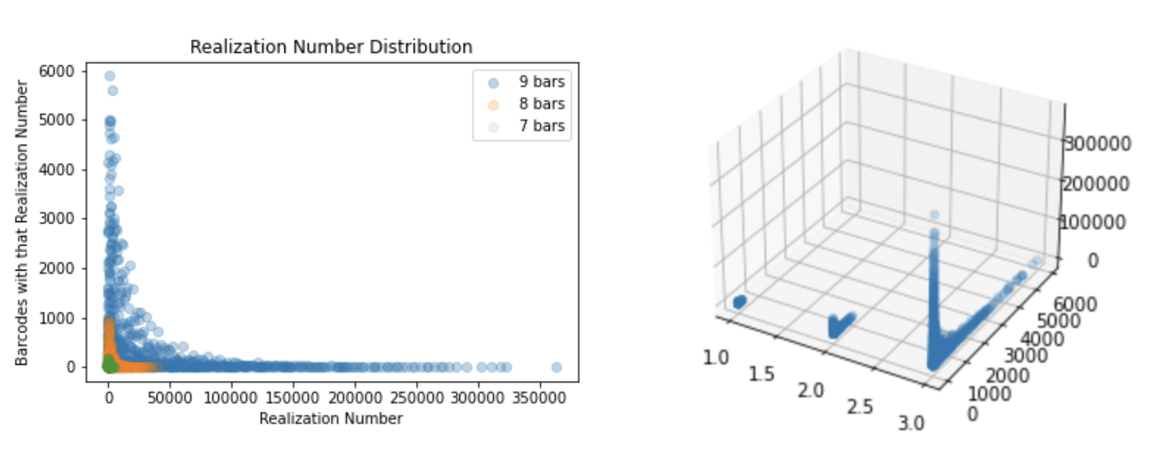
Example 4.3.
We now explicitly describe for . For convenience we write the mutisets as sets with repetition. Counting the number of appearances of a number determines .
| (10) | ||||
| (11) | ||||
| (12) |
To conclude this section, we consider the moments of . We explicitly calculate its first and second moments, obtaining the mean and variance of as corollaries, and outline a general formula for the higher moments.
Proposition 4.4.
.
Proof.
Proposition 4.5.
Proof.
We prove the result by induction on . The base case () holds trivially, so assume that the formula holds for .
Consider . Since
to prove our result, we need only show that
We call the quantity on the left :
By the sum of squares formula, we can rewrite this as
∎
Corollary 4.6.
Remark 4.7 (Higher Moments of the TRN).
In general, we can define the -th moment by rewriting and using this recursive relationship to compute a formula. We note that by Faulhaber’s formula,
where is the Bernoulli number.
One can view the results above as a complete characterization of TRNs under the null hypothesis that combinatorial classes of barcodes are distributed uniformly or as part of the growing literature on statistics on the symmetric group, see e.g., [18]. In the following section, we investigate another such statistic.
4.3. Distributions of Log Realization Numbers
Since the maximum realization number for a barcode with non-essential bars is , it is convenient to work instead with the logarithm of the realization number, which we call the log realization number. The log realization number was used in [17] as a statistic on barcodes obtained from dendrites; see Figure 2 for a reminder. This was shown to distinguish between apical and cortical dendrites. Of course, the process of taking the logarithm affects the distribution of TRNs. Jensen’s inequality provides a way to bound the expected log realization number. In this section we compute the expected log realization number of uniformly drawn barcodes.
Proposition 4.8.
The expected log realization number for a combinatorial class of barcodes drawn from the uniform distribution on is
Proof.
Recall that the set of left inversion vectors can be coordinatized as . Since this Cartesian product has size , a uniform distribution on can be viewed as a uniform distribution on the set of left inversion vectors. The notation denotes the probability of a combinatorial equivalence class of barcodes under the uniform distribution, that is . It follows that
Since , and each coordinate in is independent, the interior sum (for fixed ) is equal to . Hence
∎
5. Conclusion
In this paper, we extended the results of [17] and [4] to provide a more precise characterization of the distribution of tree realization numbers (TRNs). This investigation led us to consider the uniform distribution on the symmetric group and the expected TRN, which in turn put us in a setting where classical results from combinatorics could be used. This extraction of the notion of a combinatorial version of a merge tree led us to understand more precisely the difference between merge trees and metric phylogenetic trees [1].
We emphasize that the TRN provides a convenient summary statistic on the space of barcodes that could lead to a better understanding of inherent biological properties of neurons. If we can identify where biological barcodes live on the space of barcodes, it opens the door to many applications such as statistics of learning of “biological” barcodes, allowing to create artificial barcodes that mimic the properties of biological ones and hence to generate neurons from them that are statistically relevant, yet express higher variability. By studying the simplest possible version of a null hypothesis—where combinatorial equivalence classes of barcodes are uniformly distributed—we are in a position to move on to study more interesting variants on the null hypothesis in TDA and explore the geometry of barcode space in even greater detail.
6. Aknowledgments
JC would like to acknowledge NSF Grant
CCF-1850052 and NASA Contract
80GRC020C0016 for supporting his research. LK was supported by funding to the Blue Brain Project, a research center of the École polytechnique fédérale de Lausanne (EPFL), from the Swiss government’s ETH Board of the Swiss Federal Institutes of Technology. AG and KH gratefully acknowledge the support of Swiss National Science Foundation, Grant No. CRSII5_177237.
References
- [1] Louis J. Billera, Susan P. Holmes, and Karen Vogtmann. Geometry of the space of phylogenetic trees. Adv. Appl. Math., 27(4):733–767, November 2001.
- [2] Michael J Catanzaro, Justin M Curry, Brittany Terese Fasy, Jānis Lazovskis, Greg Malen, Hans Riess, Bei Wang, and Matthew Zabka. Moduli spaces of morse functions for persistence. Journal of Applied and Computational Topology, 4(3):353–385, 2020.
- [3] William Crawley-Boevey. Decomposition of pointwise finite-dimensional persistence modules. Journal of Algebra and its Applications, 14(05):1550066, 2015.
- [4] Justin Curry. The fiber of the persistence map for functions on the interval. Journal of Applied and Computational Topology, 2(3):301–321, 2018.
- [5] Justin Curry, Haibin Hang, Washington Mio, Tom Needham, and Osman Berat Okutan. Decorated merge trees for persistent topology. arXiv preprint arXiv:2103.15804, 2021.
- [6] Justin Curry, Sayan Mukherjee, and Katharine Turner. How many directions determine a shape and other sufficiency results for two topological transforms. arXiv preprint arXiv:1805.09782, 2018.
- [7] Jacek Cyranka, Konstantin Mischaikow, and Charles Weibel. Contractibility of a persistence map preimage. Journal of Applied and Computational Topology, 4(4):509–523, 2020.
- [8] Paul H. Edelman. The bruhat order of the symmetric group is lexicographically shellable. Proceedings of the American Mathematical Society, 82(3):355–358, 1981.
- [9] P. Erdös, Richard K. Guy, and J. W. Moon. On refining partitions. Journal of the London Mathematical Society, s2-9(4):565–570, 1975.
- [10] Joseph Felsenstein. The Number of Evolutionary Trees. Systematic Biology, 27(1):27–33, 03 1978.
- [11] Robin Forman. Morse theory for cell complexes. Advances in Mathematics, 134(1):90–145, 1998.
- [12] Marcio Gameiro, Yasuaki Hiraoka, and Ippei Obayashi. Continuation of point clouds via persistence diagrams. Physica D: Nonlinear Phenomena, 334:118–132, 2016.
- [13] Robert Ghrist, Rachel Levanger, and Huy Mai. Persistent homology and euler integral transforms. Journal of Applied and Computational Topology, 2(1):55–60, 2018.
- [14] L. Kanari, H. Dictus, A. Chalimourda, W. Van Geit, B. Coste, J. Shillcock, K. Hess, and H. Markram. Computational synthesis of cortical dendritic morphologies. BioArXiv, June 2020.
- [15] L. Kanari, P. Dłotko, M. Scolamiero, R. Levi, J. Shillcock, K. Hess, and H. Markram. A topological representation of branching neuronal morphologies. Neuroinformatics, 16(1):3–13, Jan 2018.
- [16] L. Kanari, S. Ramaswamy, Y. Shi, S. Morand, J. Meystre, R. Perin, M. Abdellah, Y. Wang, K. Hess, and H. Markram. Objective morphological classification of neocortical pyramidal cells. Cerebral Cortex (New York, NY), 29:1719 – 1735, 2019.
- [17] Lida Kanari, Adélie Garin, and Kathryn Hess. From trees to barcodes and back again: theoretical and statistical perspectives, 2020.
- [18] Risi Kondor. Group theoretical methods in machine learning. PhD thesis, Columbia University, 01 2008.
- [19] Michael Lesnick. The theory of the interleaving distance on multidimensional persistence modules. Foundations of Computational Mathematics, 15(3):613–650, 2015.
- [20] Jacob Leygonie and Ulrike Tillmann. The fiber of persistent homology for simplicial complexes. arXiv preprint arXiv:2104.01372, 2021.
- [21] Clément Maria, Steve Oudot, and Elchanan Solomon. Intrinsic topological transforms via the distance kernel embedding. arXiv preprint arXiv:1912.02225, 2019.
- [22] D. Morozov, Kenes Beketayev, and G. Weber. Interleaving distance between merge trees. 2013.
- [23] Steve Oudot and Elchanan Solomon. Barcode embeddings for metric graphs. arXiv preprint arXiv:1712.03630, 2017.
- [24] Steve Oudot and Elchanan Solomon. Inverse problems in topological persistence. In Topological Data Analysis, pages 405–433. Springer, 2020.
- [25] Elchanan Solomon, Alexander Wagner, and Paul Bendich. From geometry to topology: Inverse theorems for distributed persistence. arXiv preprint arXiv:2101.12288, 2021.
- [26] Chenguang Xu. A correspondence between schubert cells and persistence diagrams. Master thesis, Kyoto university, Supervisor: Yasuaki Hiraoka, 2020.
- [27] Lin Yan, Yusu Wang, Elizabeth Munch, Ellen Gasparovic, and Bei Wang. A structural average of labeled merge trees for uncertainty visualization. CoRR, abs/1908.00113, 2019.